Abstract
Interior permanent magnet synchronous motors (IPMSMs) exhibit significant nonlinear electromagnetic behaviour due to the effects of saturation, cross-coupling, spatial harmonics, temperature, and iron losses. In order to effectively capture the actual electromagnetic behaviour of IPMSMs, this paper proposes an improved IPMSM nonlinear model. The proposed model is based on the nonlinear flux-linkage model and progressively incorporates the effects of spatial harmonics, temperature, and iron losses. In this paper, the discrete-time form of the improved nonlinear model is established directly. It is suitable not only for embedding into the Matlab/Simulink environment as an alternative to field circuit coupling simulation but also for deployment into field programmable gate arrays (FPGA) as the model basis for hardware-in-the-loop testing. The effectiveness and feasibility of the improved model are verified by experimental results.
1. Introduction
The electrification of transportation represents a significant trend that is evident in numerous ways, with the electrification of vehicles representing a particularly notable and clear manifestation of this phenomenon [1,2,3]. The main requirements of electric vehicle powertrains for electric traction motors are high efficiency, high power density, high robustness, and low cost. Interior permanent magnet synchronous motors are the most suitable for fulfilling the majority of these criteria and are therefore mainly used in electric drivetrains [4,5,6,7].
The mathematical model of the IPMSMs is of significant importance in the design and evaluation of IPMSMs control algorithms. On the one hand, a comprehensive knowledge of the mathematical model of the IPMSM is a prerequisite for the design of the control algorithm [8,9]. On the other hand, a high-fidelity motor model can be employed as a priori benchmark for algorithm evaluation, which can be integrated into hardware-in-the-loop (HIL) test platforms for the assessment of the performance of control algorithms [10,11,12].
The conventional abc domain and dq frame IPMSMs model is relatively simple, but it fails to consider the nonlinear effects that could have a significant impact on the IPMSMs performance. Due to the high power density requirements of automotive IPMSMs, the effect of saturation and cross-coupling on the motor model cannot be neglected. As a result of saturation and cross-coupling effects, the d- and q-axis flux-linkage of the IPMSMs are not only correlated by the currents in the respective axis directions but are also influenced by the currents in the orthogonal axis directions [13]. This implies that the d- and q-axis flux-linkage behave as nonlinear functions with respect to the d- and q-axis currents. The IPMSMs exhibit relatively large spatial harmonics in the flux-linkage and current. The spatial harmonics are primarily determined by the specific topology of the machines, including the number of stator slots, winding configurations, and the number of poles. The presence of spatial harmonics can result in distortions in the current waveform and ripples in the torque. This results in the d- and q-axis flux-linkage and torque of the IPMSMs being not only current-dependent but also behaving as a function of the rotor position. Furthermore, depending on whether the IPMSMs are in the motor or generator mode, the iron loss effect can either increase or decrease the active power, which in turn has an impact on the motor current. Especially in the high-speed region, where iron losses are high and the effect on current variation cannot be ignored [14]. In addition to the aforementioned effects, the temperature effect also has a significant impact on the performance of the IPMSMs. This is manifested by the effect of the winding temperature on the stator winding resistance and the effect of the permanent magnet temperature on the relationship between flux-linkage and current.
To incorporate the effects of saturation and cross-coupling effects into the IPMSMs model, an improved non-linear inductance model in the abc domain was proposed by Ref. [10]. The authors conducted preliminary calculations of the winding self-inductance and mutual inductance of the IPMSMs using finite element analysis software. Subsequently, the inductance data are stored in the FPGA through a set of look-up tables (LuT). Furthermore, Refs. [15,16,17] also employed the inductance LuT-based methodology to model the magnetic saturation of the motor, with the model developed in the dq frame. Regardless of whether the motor is modelled in the abc domain or in the dq frame, the inductance LuT-based methods in Refs. [10,15,16,17] employ the concept of inductance to characterise the electromagnetic relationship between the motor flux-linkage and the current. To describe the effects of saturation and cross-coupling as exhaustively as possible, a substantial number of inductance tables are required for inclusion in the model. This consequently leads to an increase in the overall complexity of the model and the quantity of data. Considering that the essence of the nonlinear relationship of the motor’s magnetic circuit is the relationship between the flux-linkage and the current, Ref. [18] proposed a nonlinear flux-linkage model based on the bidirectional mapping relationship between the flux-linkage and the current. The bidirectional mapping relationship between the current and the flux-linkage naturally accounts for magnetic saturation and cross-coupling effects. This method requires fewer data tables than the inductance LuT-based modeling approach. However, spatial harmonic effects are not taken into account in this model. In order to incorporate the influence of spatial harmonics into the model, Ref. [19] enhances the nonlinear flux-linkage model in the abc domain. Five 5-dimensional LuT (5-D LuT) are employed to describe the nonlinear behaviour due to magnetic saturation, cross-coupling, and spatial harmonic effects. In order to account for the impact of iron losses in the motor model, Ref. [20] proposed the introduction of a virtual damped winding, which allows for the simulation of the iron loss effect. An alternative approach, which is more physically meaningful, is to incorporate two additional resistors that are coupled to the total stator flux-linkage in the conventional d-axis and q-axis equivalent circuits [14,21,22,23,24]. In the d- and q-axis equivalent circuits, the iron loss resistances are connected in parallel with the back electromotive force terms. When the iron loss effect is not taken into consideration, these two resistance values are deemed to be infinite, thus allowing the stator current to exert its full potential on the stator flux. When the iron loss effect is considered, the values of these two resistors are deemed to be finite. This results in a portion of the stator current exerting influence upon the stator flux-linkage, while the remaining portion flows through the iron loss resistors. The impact of temperature effects on the IPMSM model was addressed in Refs. [25,26], which increased the number of LuTs and extended the number of table indexes to account for the temperature effect. Ref. [27] established multiple 3-D lookups from FEA results, thereby facilitating the accurate depiction of torque ripple and iron loss effects in the dq reference frame of a PMSM. However, the employment of a large number of inductance look-up tables limits the application of the model in HIL testing. In Ref. [28], a distributed parameter PMSM realization method was proposed. The proposed method reduces the use of look-up tables and the storage resources required for motor modelling. Nevertheless, the model only considers saturation, cross-coupling and spatial harmonics factors and does not address iron loss and temperature effects.
In this paper, an improved nonlinear model for IPMSM is proposed, based on the nonlinear flux-linkage model presented in Ref. [18]. The improved IPMSM model incorporates the aforementioned nonlinear effects, including saturation, cross-coupling, spatial harmonics, iron loss and temperature. A 48-slot 8-pole IPMSM prototype is used as the research object in order to provide the database for the improved nonlinear model. The electromagnetic characteristics of the IPMSM prototype are calculated using finite element analysis (FEA) software Ansys Electronics 2021, which allows for the effects of the nonlinear factors to be taken into account. The discretised form of the improved nonlinear model is built directly. It is suitable not only for embedding in the Matlab/Simulink environment as an alternative to field-circuit couple simulation but also for deployment into FPGA as the model basis for HIL testing. This paper is organized as follows: Section 2 provides a review of the conventional linear model in the dq frame. Section 3 describes in detail the development process of the improved nonlinear model. Firstly, the FEA model of the IPMSM prototype is presented. Subsequently, the nonlinear flux-linkage model is employed as the foundational framework for the progressive incorporation of the effects of magnetic saturation, cross-coupling, spatial harmonics, temperature, and iron losses. In Section 4, the improved nonlinear model is integrated into the FPGA, and HIL tests are performed based on the nonlinear model. The experimental results confirm the validity and practicality of the model. The article concludes in Section 5 with a discussion of potential topics for further research.
2. Conventional IPMSM Model
In the rotor rotating reference frame (dq frame), the conventional IPMSM model is established by the following flux-linkage, voltage, and torque equations.
where and are the stator currents in the dq frame; and represent the stator flux-linkage resulting from the combination of the stator current excitation and the permanent magnet field; is the permanent magnet flux linkage, and are the stator d- and q-axis inductances.
Equations (3) and (4) report the IPMSM voltage equations in the dq frame.
where is stator phase resistance and is the rotor electrical speed; and are the stator voltages in the dq frame.
Substituting Equations (1) and (2) into Equations (3) and (4), the voltage equation can be expressed as follows.
The electromagnetic torque can be calculated from the torque equation.
where is the number of pole pairs. Substituting Equations (1) and (2) into Equation (7), the torque equation can be expressed as
The voltage Equations (5) and (6) can be discretised by Euler method and the results are as follows:
where, represents the sampling moment number. and represent the values of the d- and q-axis voltage at the sampling moment . and represent the values of the d- and q-axis current at the sampling moment . and represent the values of the d- and q-axis current at the next sampling moment . represent the value of motor speed at the sampling moment .
Equations (9) and (10) are solved with the following results:
where is the discretised time interval (), which is the sampling period of the discrete state. Equations (11) and (12) show that the value of the d- and q-axis current at time moment can be calculated from the voltage, current, speed, and motor parameters at time moment .
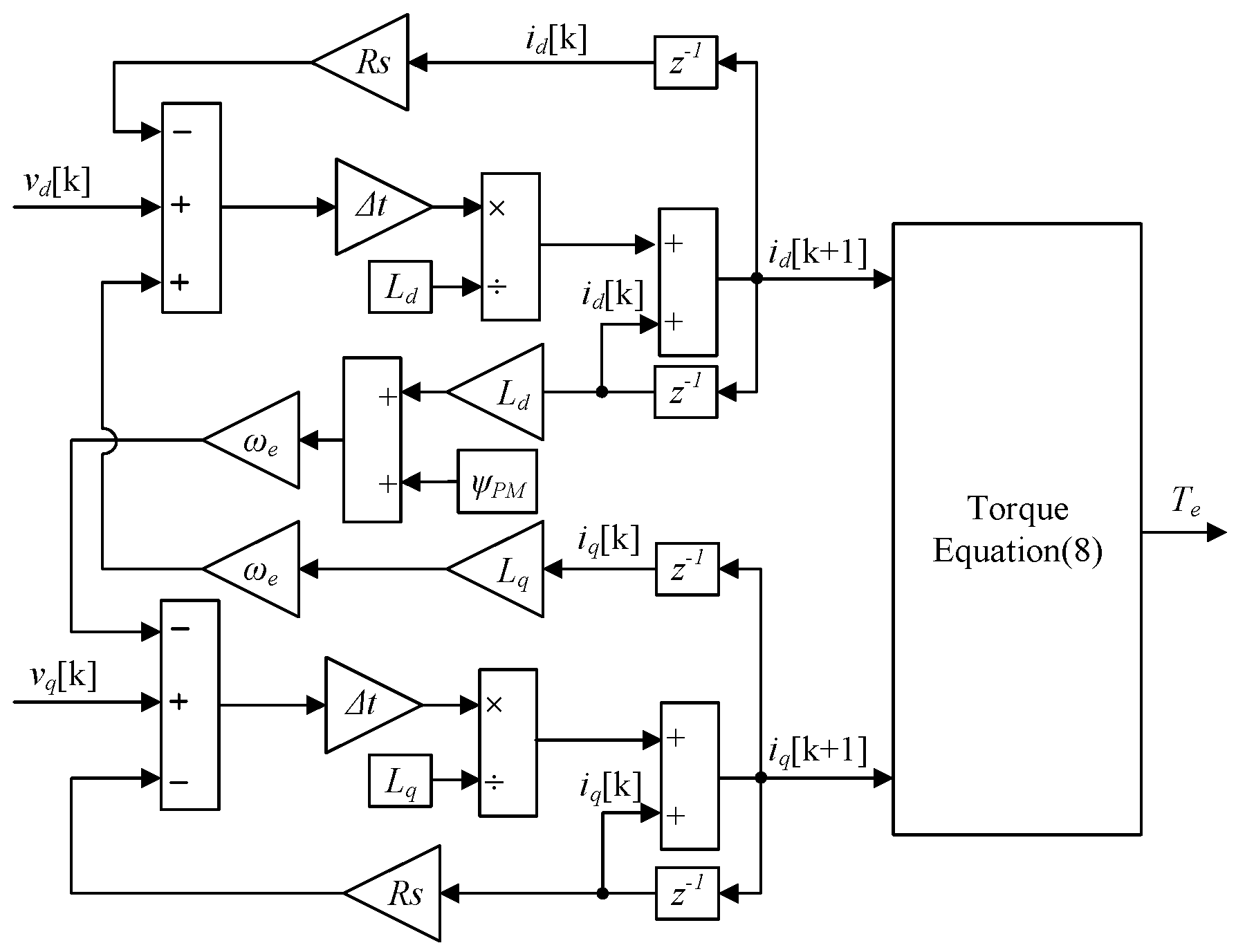
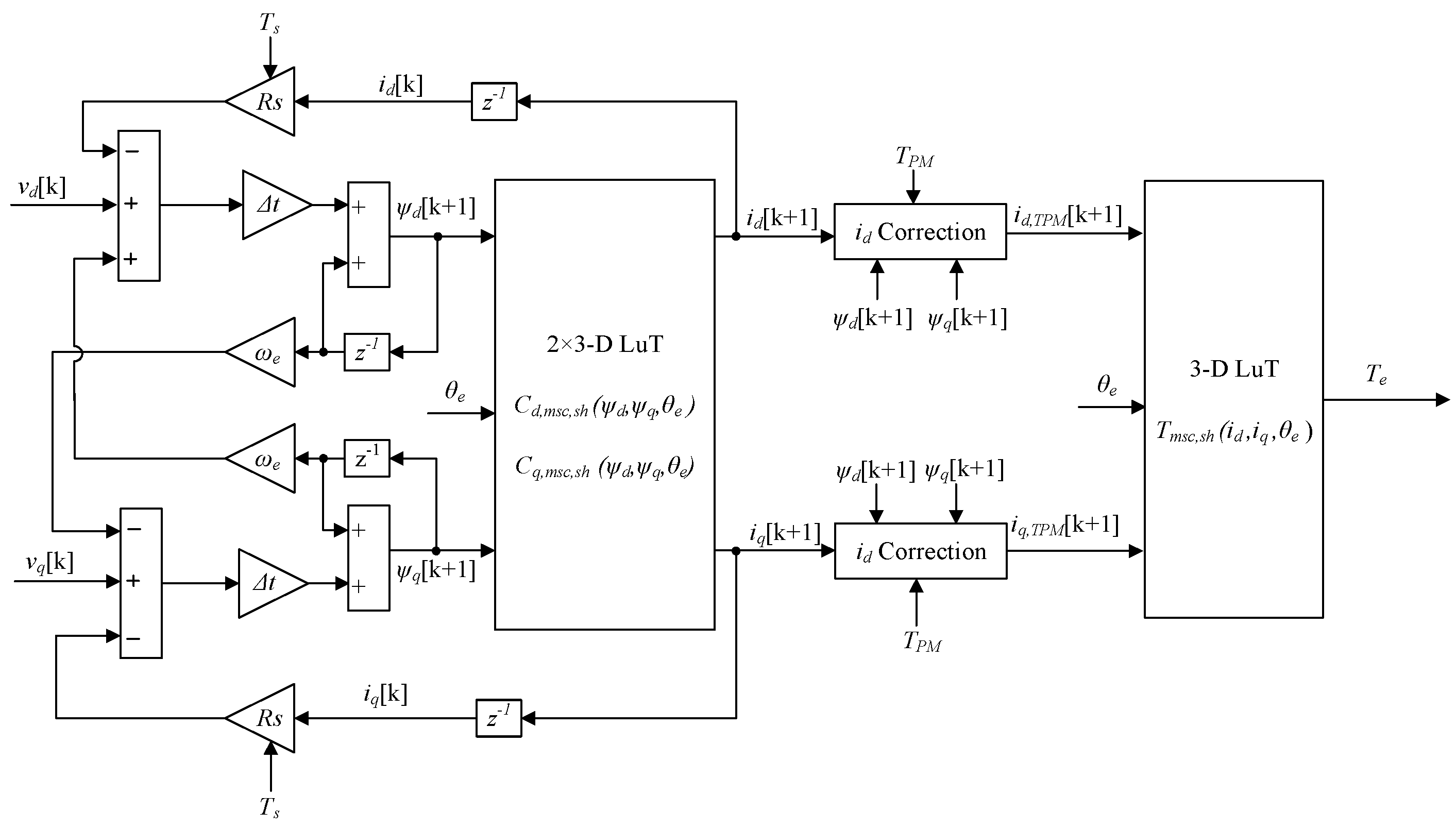
As shown in Figure 1, the discrete-time form of the conventional IPMSM model can be derived from Equations (7), (11), and (12). In Figure 1, represents the unit delay, and the delay time can be set to coincide with the discrete period of the motor model.
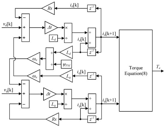
Figure 1.
Discrete-time form of the conventional (linear) IPMSM model.
3. Nonlinear IPMSM Model Considering Magnetic Saturation, Cross-Coupling, Spatial Harmonics, Temperature, and Iron Loss Effects
The nonlinear flux-linkage model is a practical modeling method that could naturally accommodate the effects of saturation and cross-coupling. In this section, the effects of spatial harmonics, temperature, and iron loss effects are introduced in a step-by-step manner on the basis of the nonlinear flux-linkage model. A high-fidelity discrete-time IPMSM nonlinear model is finally developed.
3.1. The IPMSM Prototype
In this paper, the FEA software of Ansys Electronics 2021 is used to simulate the operating characteristics of the IPMSM, incorporating considerations of saturation, cross-coupling, and spatial harmonics effect. Iron losses can be directly calculated by the software. In addition, the effect of permanent magnet temperature can be introduced by modifying the properties of the permanent magnet material. In this research, the motor is modelled and calculated in 2D due to limitations in computer computing power, thus neglecting the winding end effects.
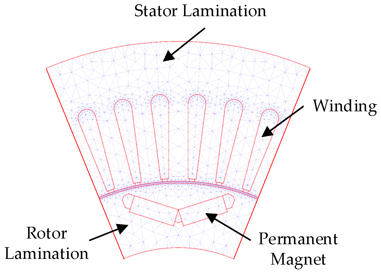
Figure 2 is the schematic of the 48-slot 8-pole IPMSM prototype (a one-eighth model). The machine design parameters are listed in Table 1.
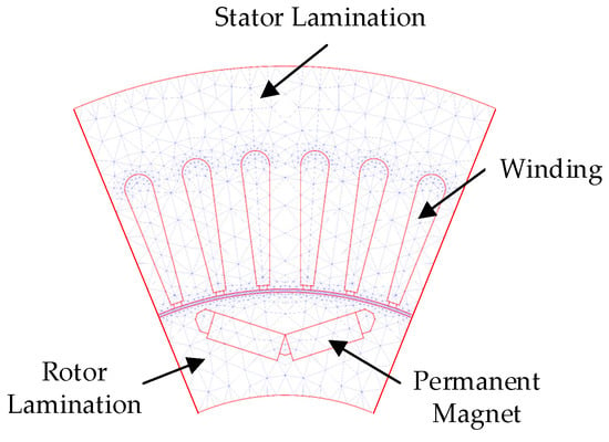
Figure 2.
Schematic of the 48-slot 8-pole IPMSM prototype (a one-eighth model).

Table 1.
Design parameters of IPMSM prototype.
3.2. Magnetic Saturation and Cross-Coupling Effects
When only the saturation and cross-coupling effects are considered, the d- and q-axis flux-linkage of the IPMSM can be identified as the average value of one electrical fundamental period. At this stage, the flux-linkage and torque are expressed only as the function of d- and q-axis currents.
where d- and q-axis flux-linkage and , respectively, are the fucntions of d- and q-axis currents and . Therefore, the effects of saturation and cross-coupling are inherently considered in the flux-linkage functions above. In this paper, these two functions are named as and . The subscripts and represent the d- and q-axis, and denotes the magnetic saturation and cross-coupling effects. At this point, the torque can still be expressed by Equation (7), except that it needs to be substituted into the non-linear flux-linkage equations shown in Equations (13) and (14).
The data for the d- and q-axis flux-linkage can be obtained by scanning the d- and q-axis currents in the FEA software. The scanning range of the is −300 A to 200 A with step 25 A. The scanning range of is from −300 A to 300 A to cover IPMSM motor and generator operation, also in steps of 25 A. Figure 3 shows the d- and q-axis averaged flux-linkage over one electrical fundamental period obtained from the FEA software.
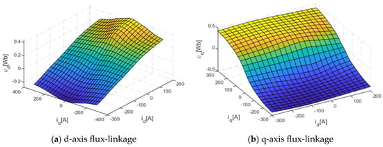
Figure 3.
The flux-linkage scanning results. (a) d-axis flux-linkage; (b) q-axis flux-linkage.
In order to establish the IPMSM model suitable for discrete-time systems, the voltage Equations (15) and (16) can be discretised by the Euler method.
where , , and represent the values of the d- and q-axis flux-linkage at the sampling moment and .
Equations (17) and (18) are solved with the following results.
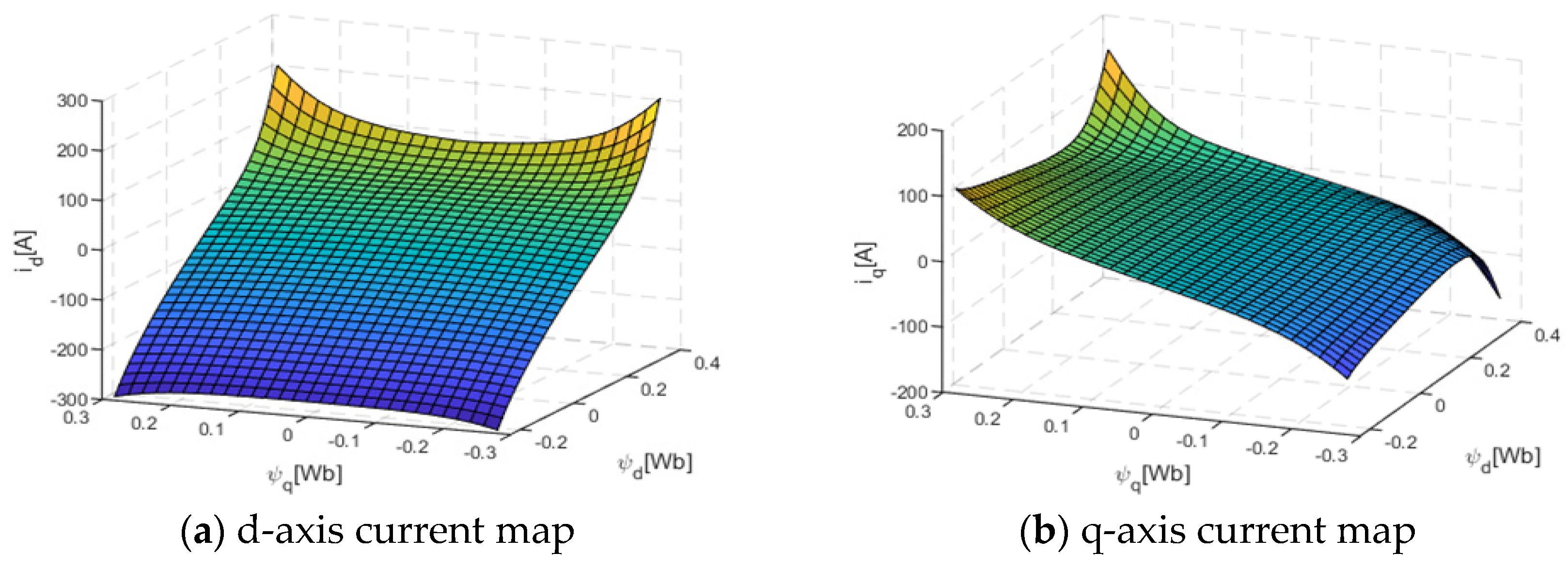
where is the discretised time interval (), which is the sampling period of the discrete state. Equations (19) and (20) show that the value of the d- and q-axis flux-linkage at time moment can be calculated by forward Euler integration with the voltage, current, flux-linkage, and speed at time moment . Due to the nonlinear relationship between the d- and q-axis flux-linkage and current, d- and q-axis currents cannot be calculated simply by the constant inductance and flux-linkage, and it is necessary to solve the inverse mapping of Equations (13) and (14) to determine the value of d- and q-axis current. The inverse mapping of current to flux-linkage can also be treated as a mapping of flux-linkage to current, and they can be represented by Equations (21) and (22) as below.
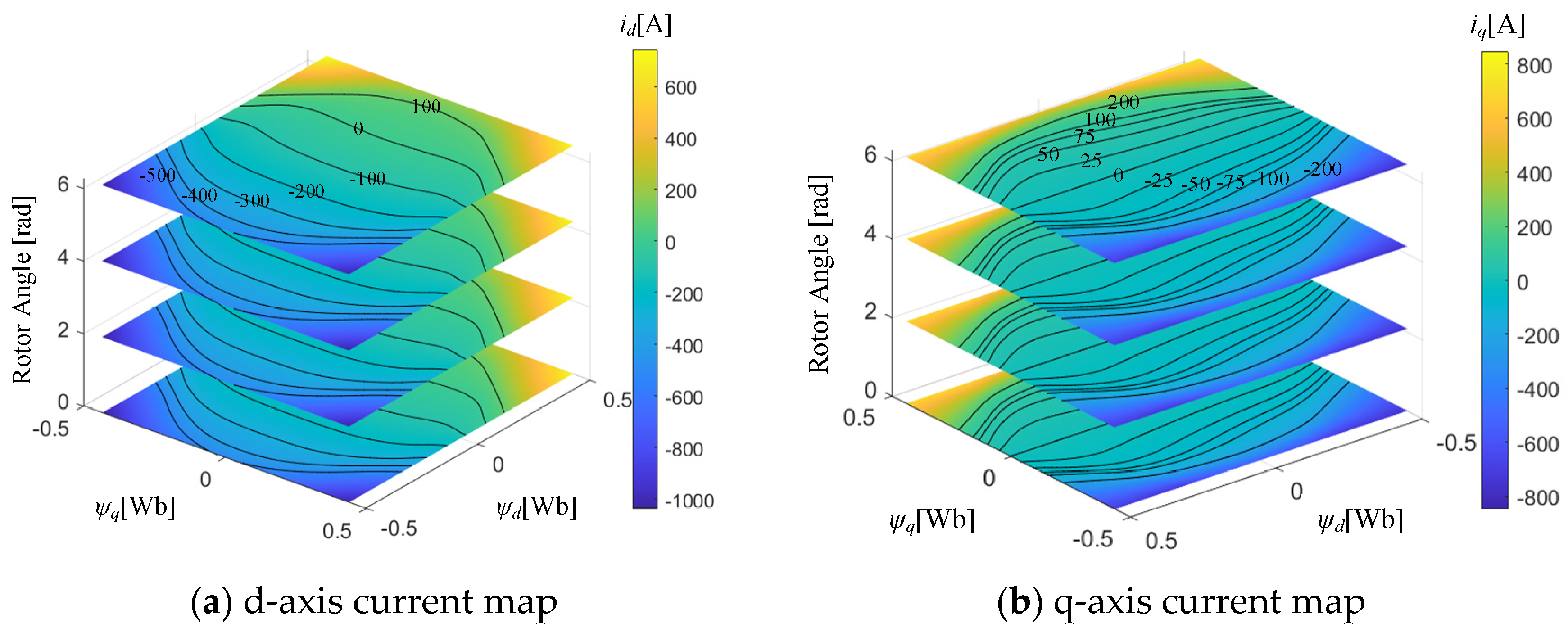
where and represent the mapping relationship from flux-linkage to current. The subscripts and represent the d- and q-axis, and denotes the magnetic saturation and cross-coupling effects. Figure 4 shows the current inverse mapping results for the average flux-linkage over one electrical fundamental period. The inverse mapping relation can be stored through the use of two 2-D look-up tables (d- and q-axis flux-linkage as indexs and d- and q-axis currents as outputs, respectively). This allows the d- and q-axis currents at any operating point to be uniquely determined.
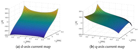
Figure 4.
The current map. (a) d-axis current map; (b) q-axis current map.
The discrete form of the IPMSM nonlinear flux-linkage model, which considers saturation and cross-coupling, can be represented by the following Figure 5, as derived from Equations (7), (19), and (20) and the two current LuTs.
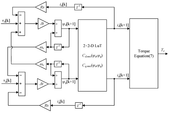
Figure 5.
Discrete-time form of the IPMSM nonlinear flux-linkage model, which considers saturation and cross-coupling.
3.3. Spatial Harmonics Effect
Due to the nonlinear characteristics of the magnetic circuit, the pole shapes, winding distributions, and cogging, the IPMSM exhibits relatively large spatial harmonics. The spatial harmonics result in a notable torque ripple due to the varying magnetic energy with rotor position. This results in flux and torque being related not only to current but also to rotor position, as shown in the following equations.
where flux-linkage and torque are the fucntions of d- and q-axis currents and and rotor position angle . These functions are named as , and here. The subscripts and represent the d- and q-axis, and denotes the magnetic saturation and cross-coupling effects. denotes that the spatial harmonic effect is considered here. Correspondingly, the flux-to-current mapping relationship also exhibits the correlation with the rotor position angle, as shown in the following equations.
where, and represent the mapping relationship from flux-linkage to current.
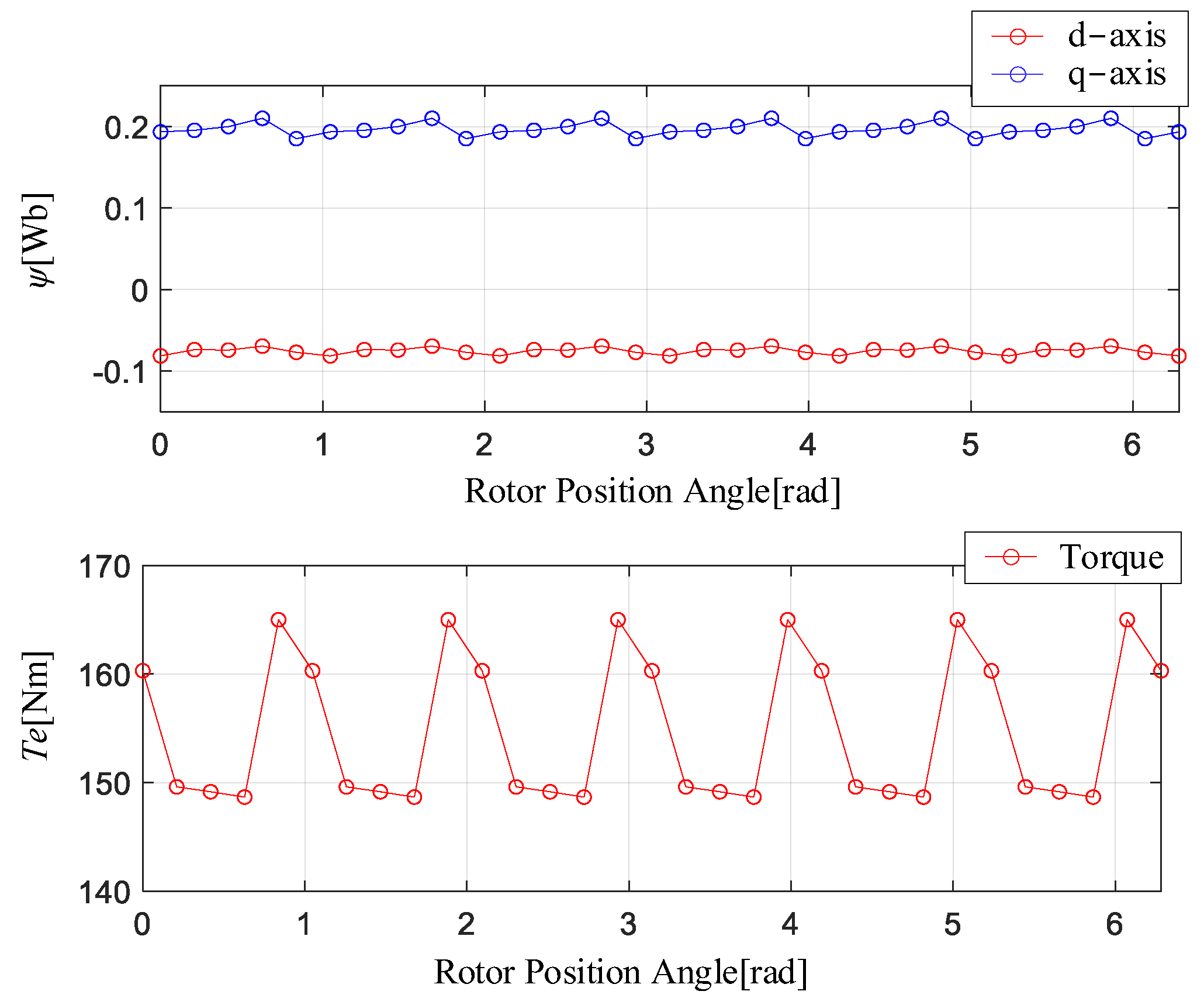
Figure 6 shows the FEA results of the flux-linkage of the d- and q-axis and the torque over one electrical fundamental period at the operating point ( = −150 A, = 50 A and = 500 RPM).
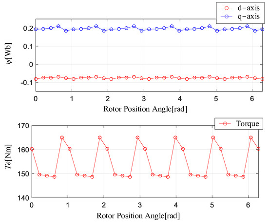
Figure 6.
Flux-linkage and torque variations with the rotor position.
As shown in Figure 6, the spatial harmonics effect results in variations in the d- and q-axis flux-linkage and torque values depending on rotor position angles. This implies that when spatial harmonics effects are incorporated into the IPMSM nonlinear model, the solution of the flux-linkage to current mapping needs to be performed at different rotor position angles. Consequently, the 2-D LuT is extended to a 3-D LuT (with the addition of the rotor position angle as a new index). The flux-linkage and torque data for different rotor positions can be obtained by scanning the rotor position angle in the FEA software.
A part of the results of solving the flux-linkage to current mapping at different rotor positions are shown in Figure 7, and Figure 7 only shows the results of the solution at the 4 rotor positions (a range of electrical angles from 0° to 360° with a step size of 120°).
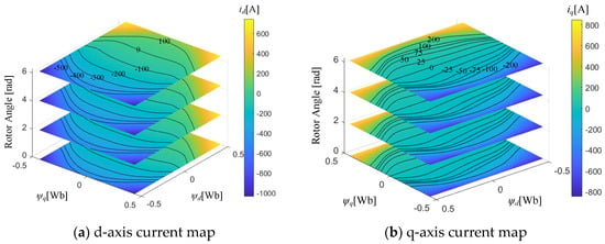
Figure 7.
Current maps versus the d-and q-axis flux-linkages at different rotor positions. (a) d-axis current mapping; (b) q-axis current map.
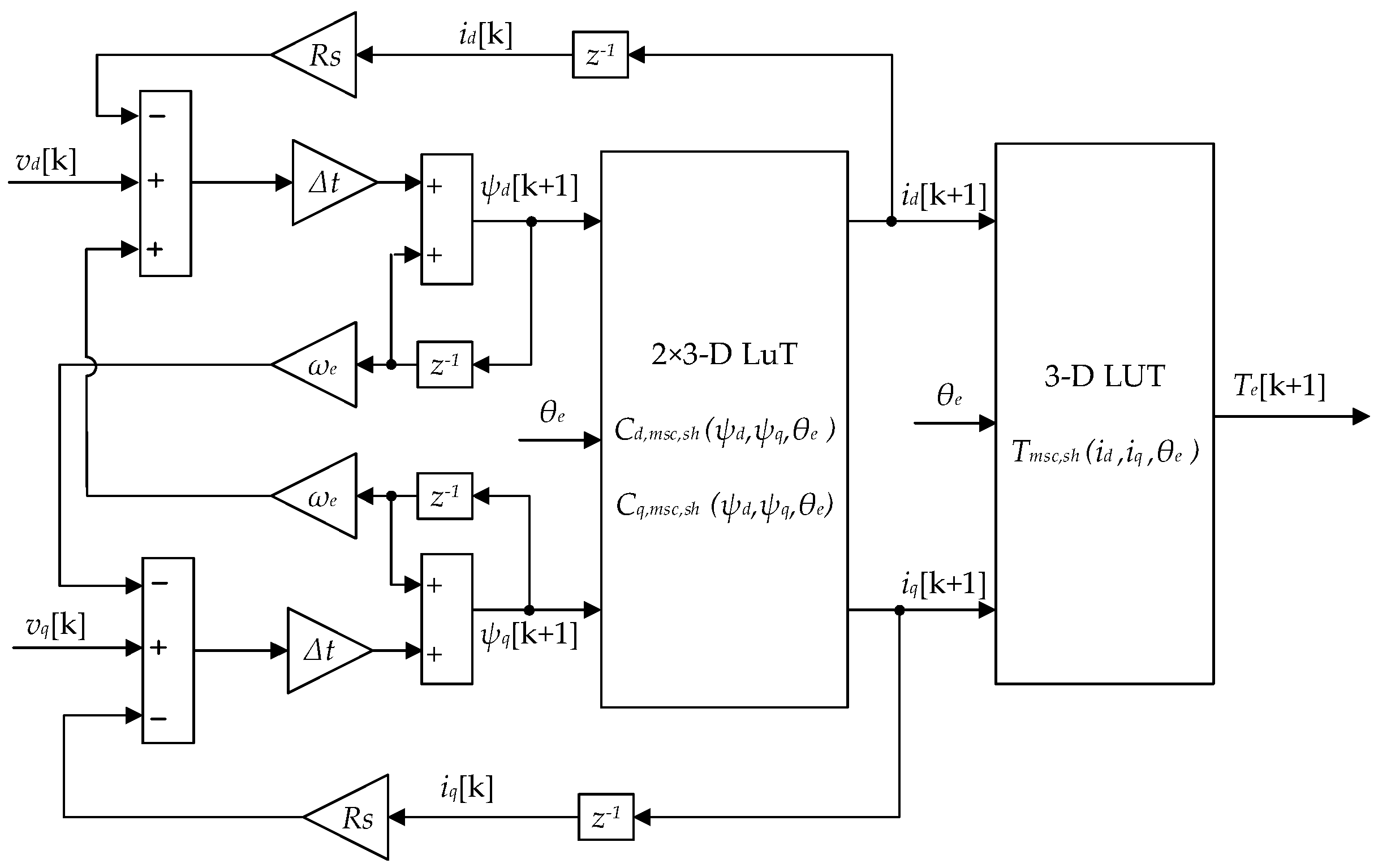
Based on the above analysis, the discrete form of the IPMSM nonlinear model considering saturation, cross-coupling, and spatial harmonic effects can be constructed as shown in Figure 8.

Figure 8.
Discrete-time form of the IPMSM nonlinear flux-linkage model, which considers saturation, cross-coupling and spatial harmonics.
3.4. Temperature Effect
The temperature effect on the IPMSM nonlinear model is characterised by two specific aspects: the effect of the winding temperature on the stator winding resistance and the effect of the permanent magnet temperature on the relationship between flux and current. During the operation of IPMSM, the temperature at the ends of the windings is typically higher than the temperature in the stator slots. However, for the sake of simplicity, it is assumed that the temperature of the stator winding is uniformly distributed. According to this assumption, the stator winding resistance can be calculated for a given winding temperature by the following equation.
where is the reference temperature in FEA software, which is set to 20 °C. In the proposed improved IPMSM model, the temperature is fixed and serves as the reference temperature for the calculation of winding resistance. is the resistance at reference temperature. represents the temperature set for the stator winding in the IPMSM model. This temperature can be set artificially. is the temperature coefficient of resistance.
The properties of permanent magnet materials do vary with temperature, which correspondingly affects the relationship between d- and q-axis currents and flux-linkage. This implies that Equations (23) and (24) are to be further expanded with respect to the permanent magnet temperature .
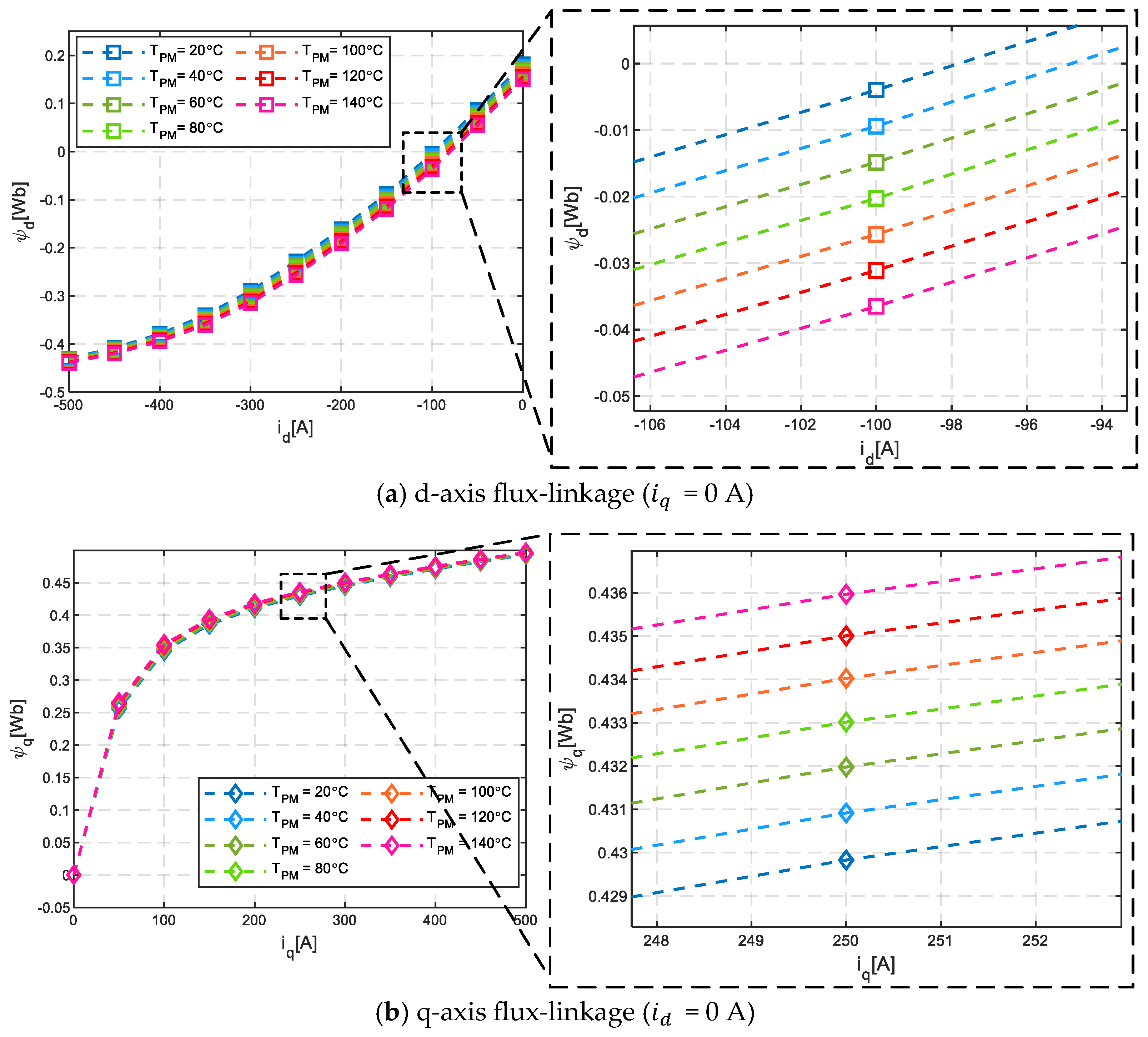
where, d- and q- axis flux-linkage are the fucntions of d- and q-axis currents and , rotor position angle and permanent magnet temperature . These functions are named as and here. The subscripts and represent the d- and q-axis, and denotes the magnetic saturation and cross-coupling effects, denotes that the spatial harmonic effects and represent the temperature effects. The influence of the permanent magnet temperature effect in the FEA calculation can be introduced by modifying the permanent magnet material properties according to Ref. [29]. Figure 9 shows the FEA results of d-axis and q-axis flux-linkage at different permanent magnet temperature conditions. For the sake of clarity, only the average value of the flux-linkage over one electrical fundamental period is considered here. From the figure, it can be observed that the change of permanent magnet temperature results in a shift in the d- and q-axis flux-linkage for the same current operating point. This is because the permanent magnet temperature directly affects the residual magnetization of the permanent magnet, which in turn affects the d- and q-axis flux-linkage. While the magnitude of the flux-linkage shift may be small, even a slight flux-linkage change has the potential to induce a significant voltage error under high-speed operating conditions.
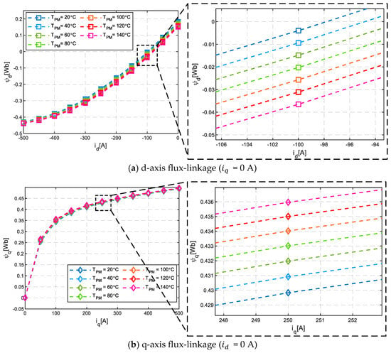
Figure 9.
Flux-linkage at different permanent magnet temperature conditions: (a) d-axis flux-linkage; (b) q-axis flux-linkage.
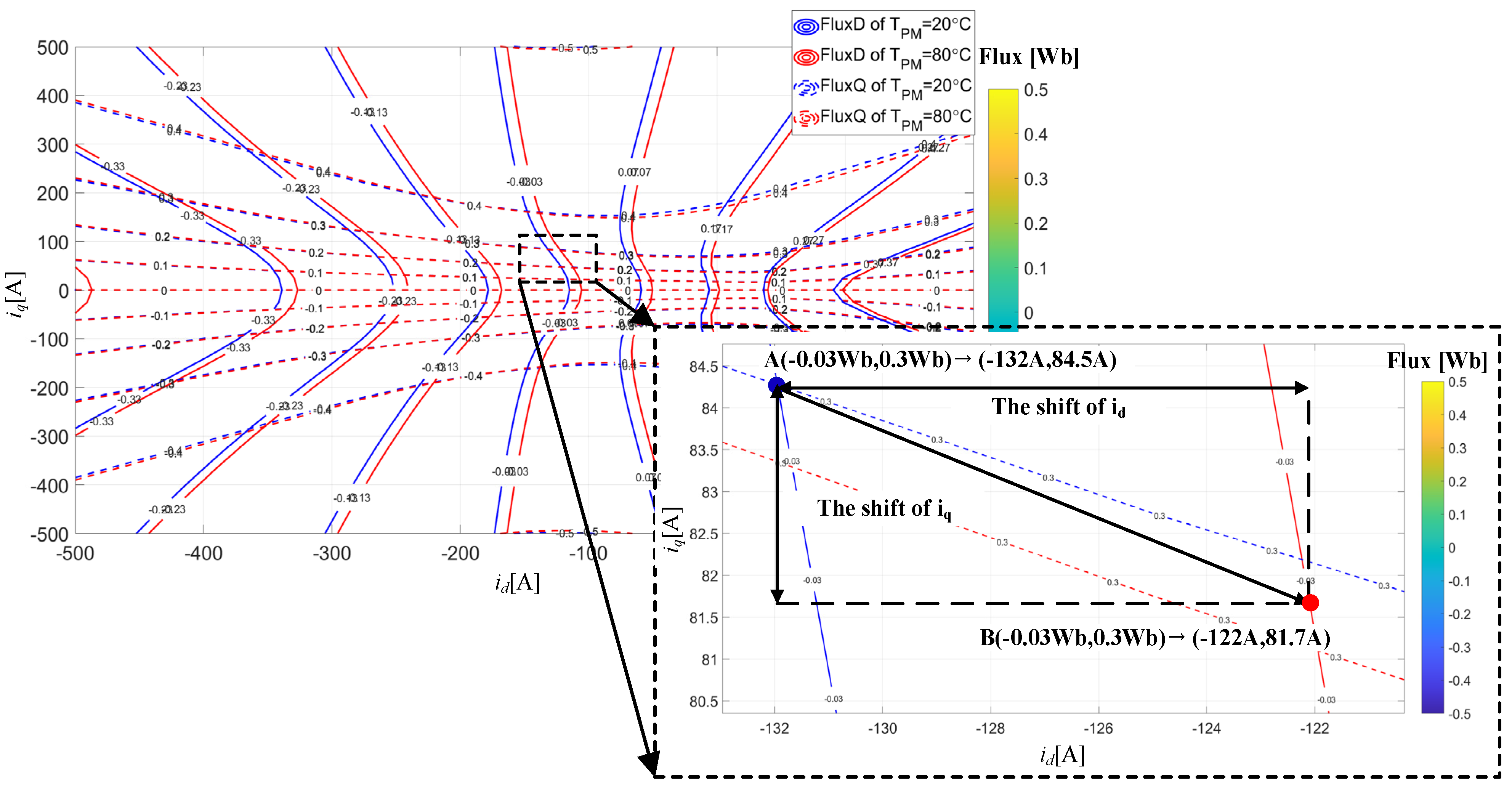
A more intuitive and practical shift illustration can be described with flux-linkage contour lines in the d-q current plane, as shown in Figure 10. In Figure 10, the blue solid lines are the contours of the d-axis flux-linkage at 20 °C permanent magnet temperature. The solid red lines are the contours of the d-axis flux-linkage at 80 °C permanent magnet temperature. The blue dash lines are the contours of the q-axis flux-linkage at 20 °C permanent magnet temperature. The red dash lines are the contours of the q-axis flux-linkage at 80 °C permanent magnet temperature. The numbers on the contour lines indicate the value of the flux-linkage. In the zoomed-in illustration, point A (blue, 20 °C) and point B (red, 80 °C) have the same flux-linkage value, but there is a significant current shift between the two points. This means that for the discrete IPMSM model shown in Figure 8, a current shift module needs to be added after the current LuT signal flow to reflect the effect of permanent magnet temperature. The current shift can be decomposed into the d- and q-axis direction, denoted as d-axis current shift and q-axis current shift, respectively. The d-axis current shift and the q-axis current shift are functions of d- and q-axis flux-linkage and permanent magnet temperature. In this paper, the effect of permanent magnet temperature variations is processed through a linear relationship and the d- and q-axis current shift and for the given permanent magnet temperature can be calculated as Equations (31) and (32). More details of these current shift equations are further discussed in Appendix A.
where is the temperature set for the permanent magnet in the IPMSM model, and are the base values of the current shift, and the data for these two base values can be calculated by FEA results at permanent magnet temperatures of 20° and 80°, respectively. is the base values of temperature variance. This value corresponds to the temperature at which the current reference value is calculated. Figure 11 shows the results of these two base values, which can be stored in two 2-D LuTs in the IPMSM model.
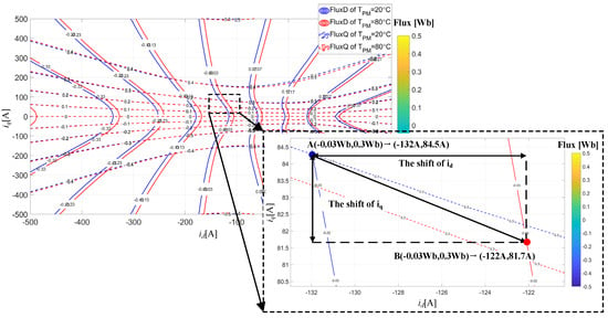
Figure 10.
Illustration of the permanent magnet temperature factor on the flux-current relationship.
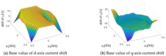
Figure 11.
Base value of d-and q-axis current shift: (a) Base value of d-axis current shift; (b) Base value of q-axis current shift.
Based on Equations (31), (32), and the base values of the d-axis and q-axis current shift, the d-axis and q-axis currents can be calculated for the given permanent magnet temperature by the following equations.
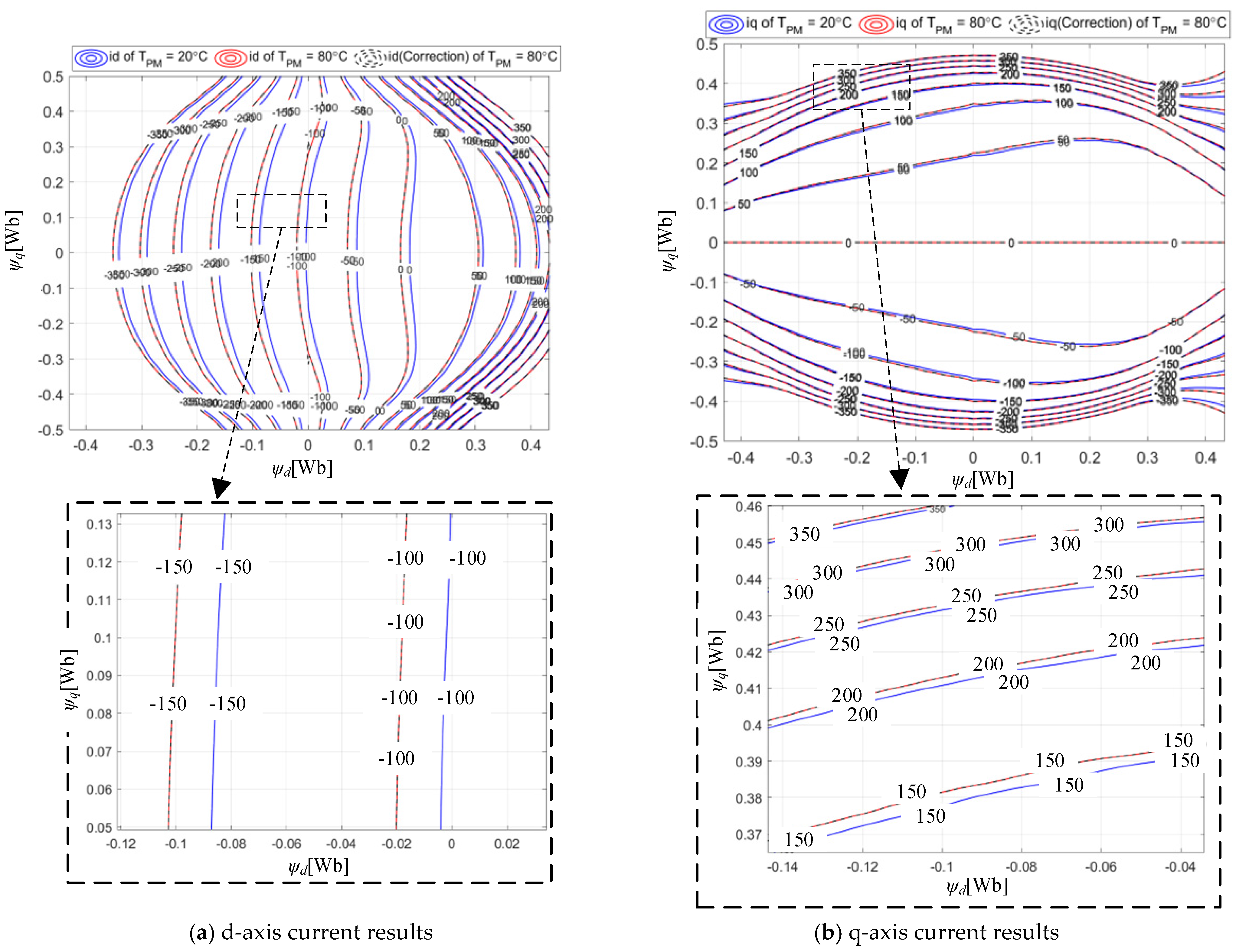
where, and are the results of the 3-D current LuT and . The subscript 20 °C indicates that the data in the LuT are the FEA results at 20 °C permanent magnet temperature. and are current corrections calculated for a given temperature. is the permanent magnet temperature. Figure 12 shows the comparison of the FEA results with the current correction results calculated according to Equations (33) and (34).
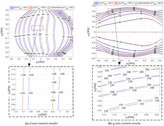
Figure 12.
Comparison of FEA results with current correction results: (a) d-axis current results; (b) q-axis current results.
In Figure 12, the blue solid lines are the current contour lines of FEA results for the 20 °C permanent magnet temperature condition, the red solid lines are the current current contour lines of FEA results for the 80 °C permanent magnet temperature condition, and the black dashed lines are the current correction results calculated according to Equations (34) and (35). As illustrated in the figure, the current corrections exhibit a good degree of concordance with the FEA results.
Based on the above analysis, the discrete form of the IPMSM nonlinear model considering saturation, cross-coupling, spatial harmonic, and temperature effects can be constructed as shown in Figure 13.
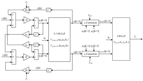
Figure 13.
Discrete-time form of the IPMSM nonlinear flux-linkage model, which considers satu-ration, cross-coupling, spatial harmonics and temperature effects.
3.5. Iron Loss Effect
The conventional d- and q-axis equivalent circuit which takes into account the iron loss effect of the IPMSM is presented in Ref. [21]. Two additional resistances are inserted in parallel to the induced voltages into the equivalent circuits. In this paper, some improvements have been made to the circuit as shown in Figure 14. In order to introduce magnetic saturation effects, a replacement of the transformer electromotive force term characterized through the inductive voltage with the differentiation of the flux-linkage is made. The speed electromotive force term is also calculated directly from flux-linkage.

Figure 14.
Equivalent circuit with iron loss effect. (a) Equivalent circuit of d-axis with iron loss effect. (b) Equivalent circuit of q-axis with iron loss effect.
By applying Kirchhoff’s voltage law to the closed circuit S1 and S3 in Figure 15, it can be verified that Equations (15) and (16) remain valid. This indicates that the flux-linkage calculation in the previous IPMSM models does not require modification. However, the application of Kirchhoff’s current law to points P1 and P2 reveals that the axis total current ( and ) is now split into two components: the iron loss current component ( and ) and the magnetization current component ( and ). It is assumed that and depend only on the magnetization current components. Under this assumption, the current inverse mapping LuT in the previous IPMSM models remains valid. However, in order to introduce the effect of iron losses, it is necessary to add an additional iron loss current calculation module to the IPMSM model. This is due to the fact that the additional iron loss current results in an increase in the voltage drop across the stator winding resistors on the d- and q-axis of the equivalent circuit, which induces a shift in the voltage components and .
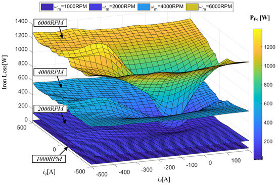
Figure 15.
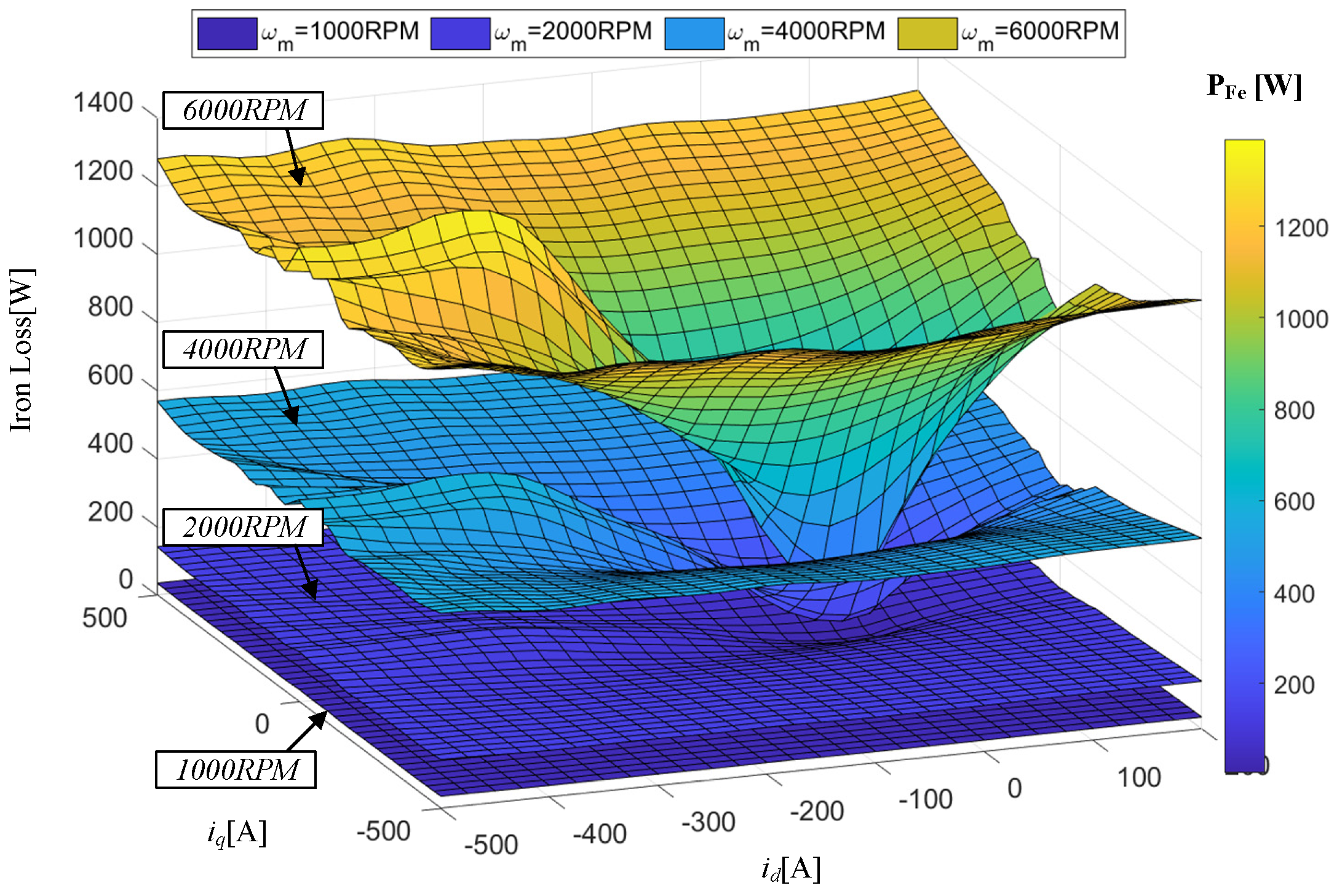
Results of the iron loss FEA calculation.
The iron loss current and can be calculated based on the equivalent circuit and the iron loss power. As the iron loss power (including eddy current losses and hysteresis losses) can be derived as a basic output term from the FEA software, it is a relatively straightforward process to determine the iron loss current. Considering the steady state condition, the dynamic voltage terms and can be neglected. When Kirchhoff’s voltage law is applied to S2 and S4, the following equations are obtained.
Equations (35) and (36) represent the voltage drop across the d-axis and q-axis iron loss resistors. According to the equivalent circuit shown in Figure 14, the iron loss power in the d- and q-axis can be expressed as follows.
According to Equations (37) and (38), the iron loss current can be calculated as follows.
where, the values of and are known and can be obtained from the aforementioned flux-linkage calculation module. is the electrical speed of IPMSM. d- and q-aixs iron loss and can be determined according to the following equation.
where is d-axis component of the eddy current loss, is d-axis component of the hysteresis loss, is q-axis component of the eddy current loss, is q-axis component of the hysteresis loss. , , and are relative iron loss factors, and they are defined by as below according to Ref. [23].
The physical meaning of this definition is that hysteresis losses depend on the flux in the same direction, while eddy current losses depend on the flux in the orthogonal axis direction. This is because the induction effect always produces a current orthogonal to the field source. Based on Equations (39)–(46), the d- and q-axis iron loss currents can be calculated as follows.
In Equations (47) and (48), the data of eddy current loss and hysteresis loss can be obtained by post-processing in FEA software. In order to reduce the complexity of the IPMSM nonlinear model, it is possible to consider only the average value of the iron losses over one electrical fundamental period. This results in the elimination of the rotor position angle, which implies that the iron loss is only the function of the axis current and the motor speed.
The FEA results for the iron losses are shown below. This data can be stored through a 3-D LuT in the IPMSM nonlinear model.
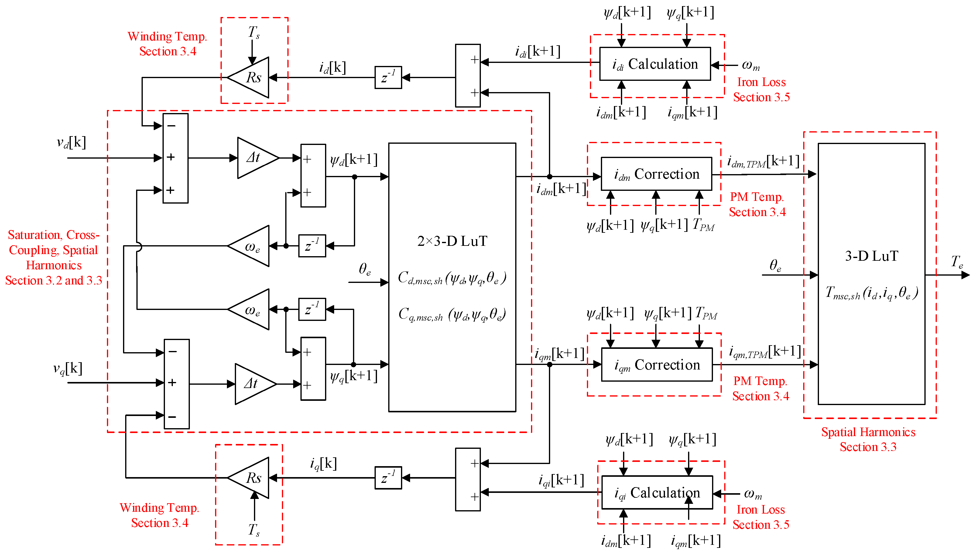
The nonlinear discrete model of the IPMSM, which takes into account saturation, cross-coupling, spatial harmonics, temperature, and iron loss effects, can be developed based on the analyses presented in Section 3.2, Section 3.3, Section 3.4 and Section 3.5. Figure 16 shows the overall structure of the IPMSM nonlinear model. In the diagram, the important modules are labelled with red dash boxes, with the corresponding chapter numbers next to the box lines.
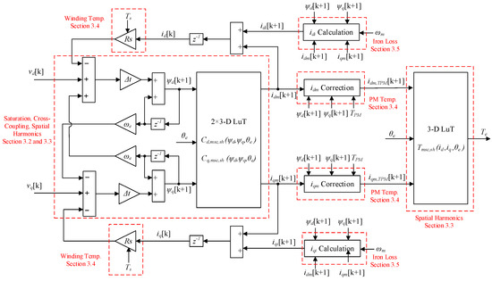
Figure 16.
Discrete-time form of the IPMSM nonlinear flux-linkage model, which considers saturation, cross-coupling, spatial harmonics, temperature, and iron loss effects.
4. Hardware-in-Loop Verification
4.1. Test Platform
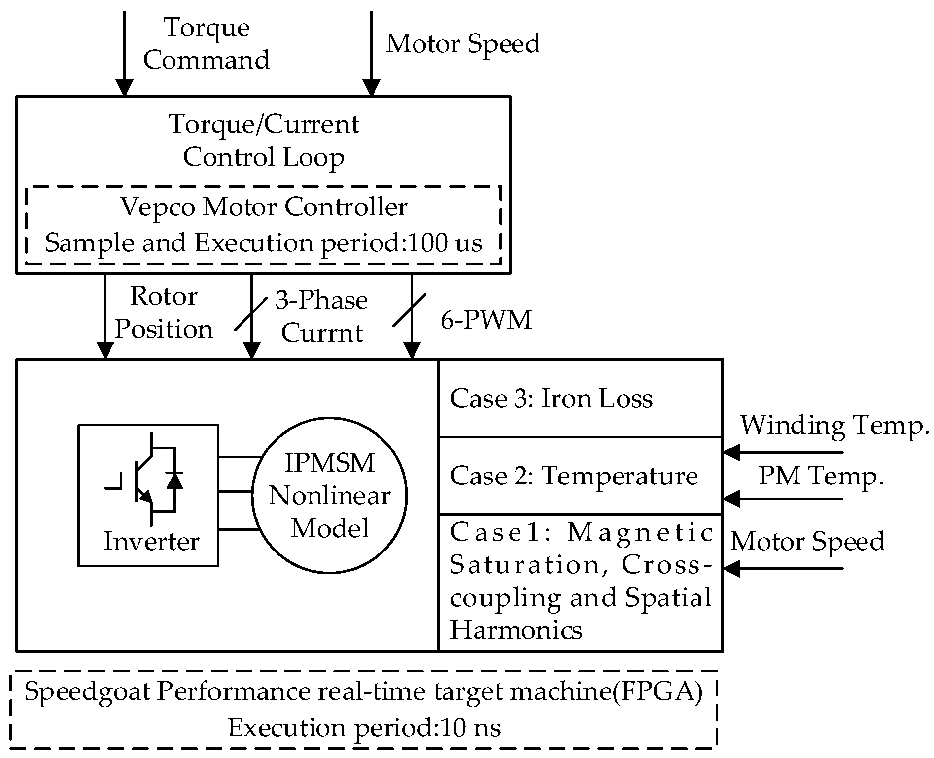
The HIL test platform based on the Speedgoat Performance real-time target machine is employed to validate the improved IPMSM nonlinear model proposed in this paper. Figure 17 shows the schematic diagram and the photograph of the test platform. The main hardware components of the real-time test platform are the real-time target machine with integrated FPGA board provided by Speedgoat GmbH, a motor controller and signal converter board provided by VEPCO Technologies Inc, a CAN bus communication board provided by Vector Informatik GmbH, and host computers. The software environment consists of the following programs. Matlab/Simulink R2024a was employed for the development of the IPMSM nonlinear model, as well as for the graphical analysis of the test results. The HDL Coder toolbox embedded in Matlab and Vivado Design Suite 2022.1 from Xilinx Inc. was used to implement the nonlinear model in the FPGA without hand-coding the hardware description language. The Matlab Fixed-Point Tool was used to perform the fixed-point implementation of the IPMSM model in floating-point form.

Figure 17.
Schematic diagram and photograph of the test platform: (a) Schematic diagram, (b) Photograph.
The principle and structure of the IPMSM nonlinear model shown in Figure 17 are based on the discrete time form of the IPMSM nonlinear model shown in Figure 8, Figure 13, or Figure 16 to accommodate different nonlinear factors. The feasibility and performance of the nonlinear model are validated through three test cases that progressively incorporate the aforementioned nonlinear effects. Figure 18 is the schematic diagram of these test cases. Case 1 aims to examine the verification of magnetic saturation, cross-coupling, and spatial harmonic effects. In Case 1, the fundamental principles and structural framework of the IPMSM nonlinear model are illustrated in Figure 8, with the temperature and iron loss effects not included. Case 2 examines the validation of the temperature effect. In Case 2, the principle and structure of the IPMSM nonlinear model are shown in Figure 13. The temperatures of the stator winding and the permanent magnet are set by the host computer. Case 3 is for the validation for the iron loss effect, and the principle and structure of the IPMSM nonlinear model are shown in Figure 16.
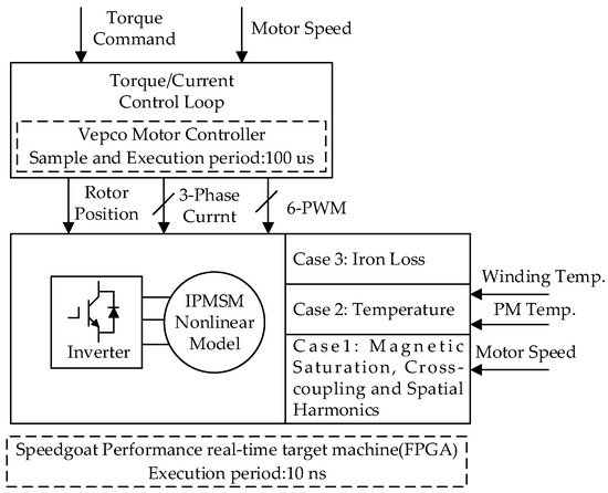
Figure 18.
Schematic diagram of the test cases.
4.2. Case 1: Validation of Magnetic Saturation, Cross-Coupling, and Spatial Harmonic Effect
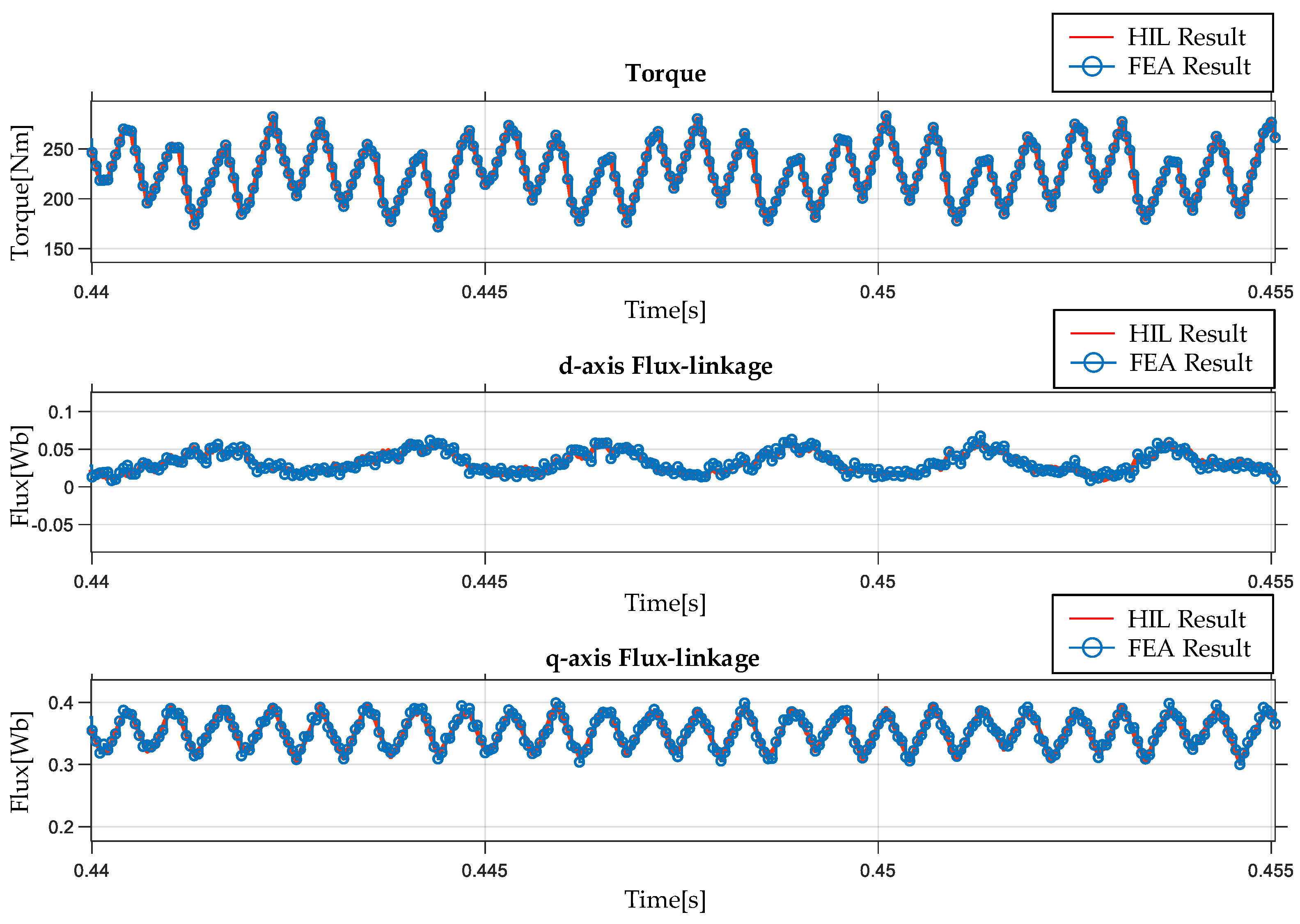
A single operating condition is employed to validate the saturation, cross-coupling, and spatial harmonic effects. The motor speed is set by the host computer in order to simulate the operation that the IPMSM under test is driven by the dynamometer. The motor speed is set to 1000RPM. The motor controller is operating in torque control mode, and the sampling and execution period is 100 μs, corresponding to the PWM frequency of 10 kHz. The torque command is set at the rated motor torque of 230 Nm. The IPMSM model is executed in the Speedgoat Performance real-time target machine with an execution time of 1 μs. The results of the HIL test for this operating condition are shown in Figure 19.
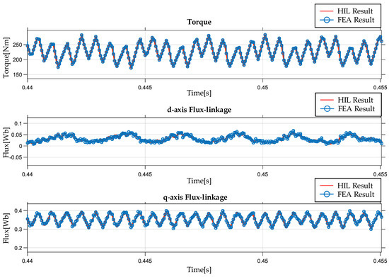
Figure 19.
Torque and flux-linkage test results for one electrical period.
To compare the HIL test results with the FEA calculation results, the d- and q-axis current data are extracted from the HIL test results and then injected as excitation into the FEA model. The torque results obtained from the FEA are compared with the HIL test results. As can be seen in Figure 19, the difference between the two results is insignificant. This is due to the fact that the motor torque depends on the current and the flux-linkage, whereas the flux-linkage and current data in the IPMSM model of the HIL test have been previously calculated by the FEA software. Consequently, there is a good match between the two sets of results under the same operating conditions. This implies that the improved IPMSM model is capable of incorporating the effects of saturation, cross-coupling, and space harmonics factors into the HIL test model, thereby enhancing the fidelity of the HIL test.
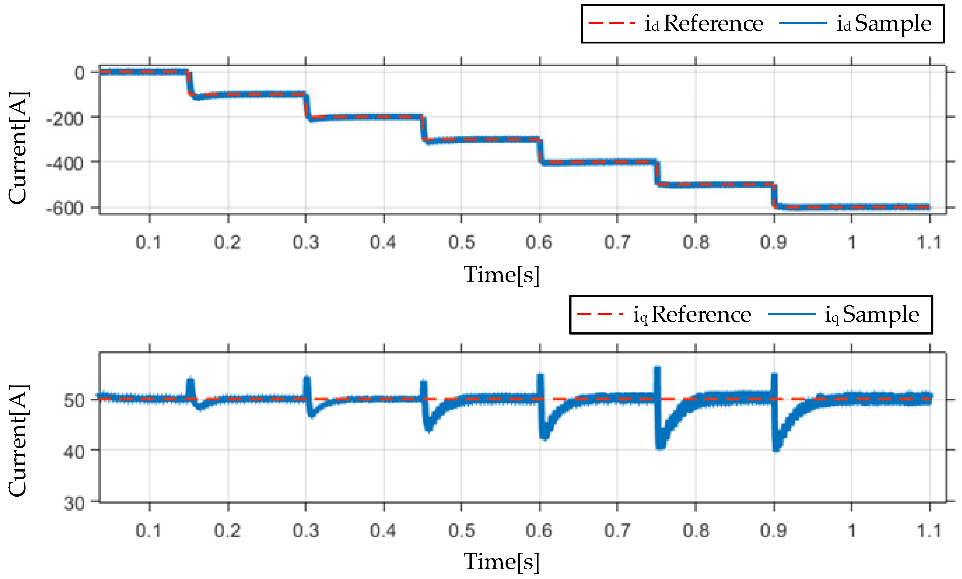
Figure 20 shows the results of current control tests with the nonlinear motor model, which indicate the applicability of the model for transient state analysis. The motor speed is maintained at 500 RPM, the q-axis current reference is maintained at 50 A, and the d-axis current reference decreases in steps of −100 A until it reaches twice the rated current to adequately account for the saturation and cross-coupling factors. From the test results, it can be seen that due to the cross-coupling factor, the variation of the d-axis current reference not only affects the results of the d-axis current control but also has an impact on the q-axis current. Meanwhile, the effect of the cross-coupling factor on the current control results becomes increasingly significant with the rise in the stator current amplitude.
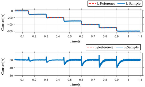
Figure 20.
Current control test results.
4.3. Case 2: Validation of Temperature Effect
In the HIL test, verification of the effect of temperature, a single operating condition is selected for the purpose of verifying the effect of different winding temperatures and permanent magnet temperatures on the motor torque. Subsequently, the external characteristics of the motor under different temperature conditions are compared.
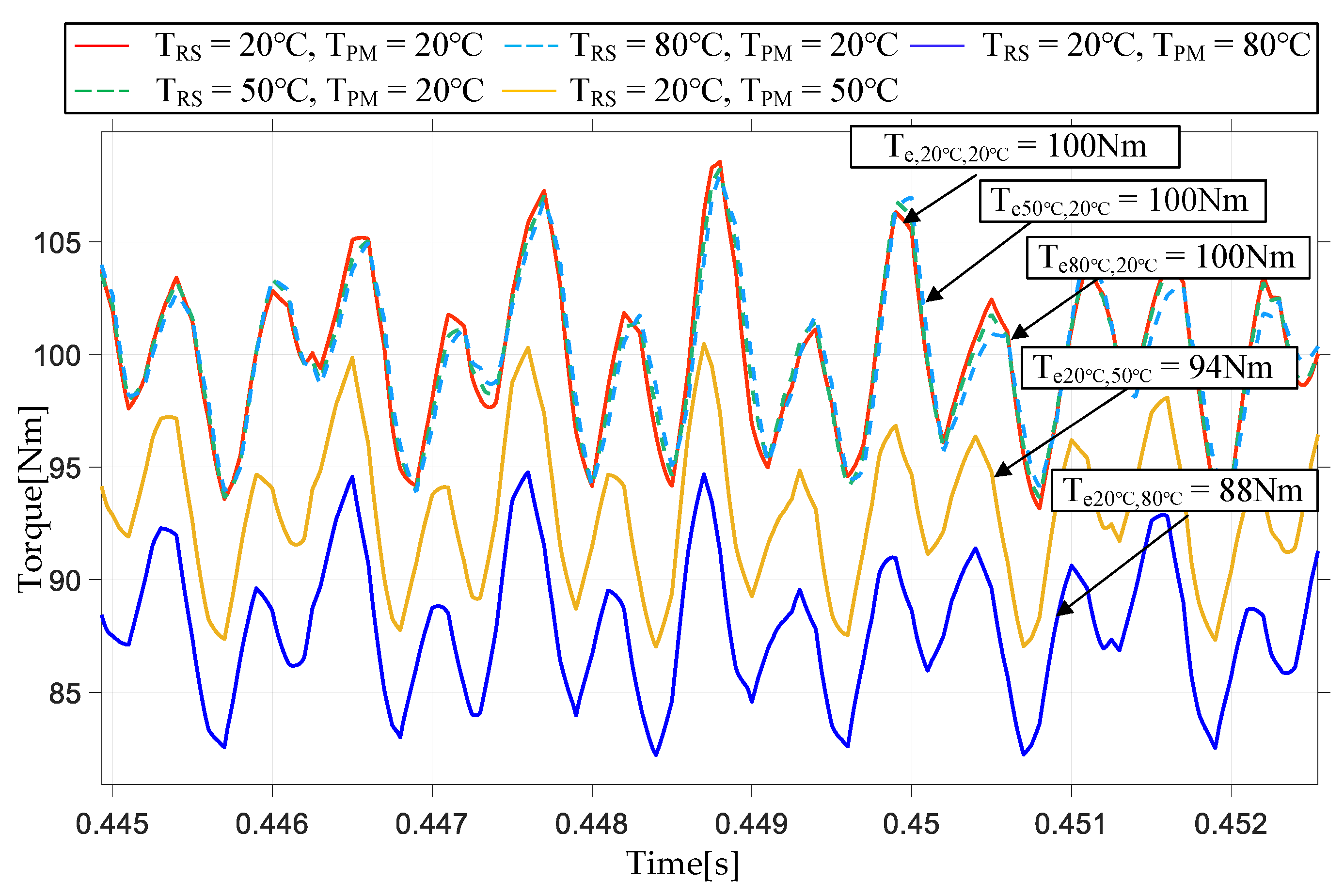
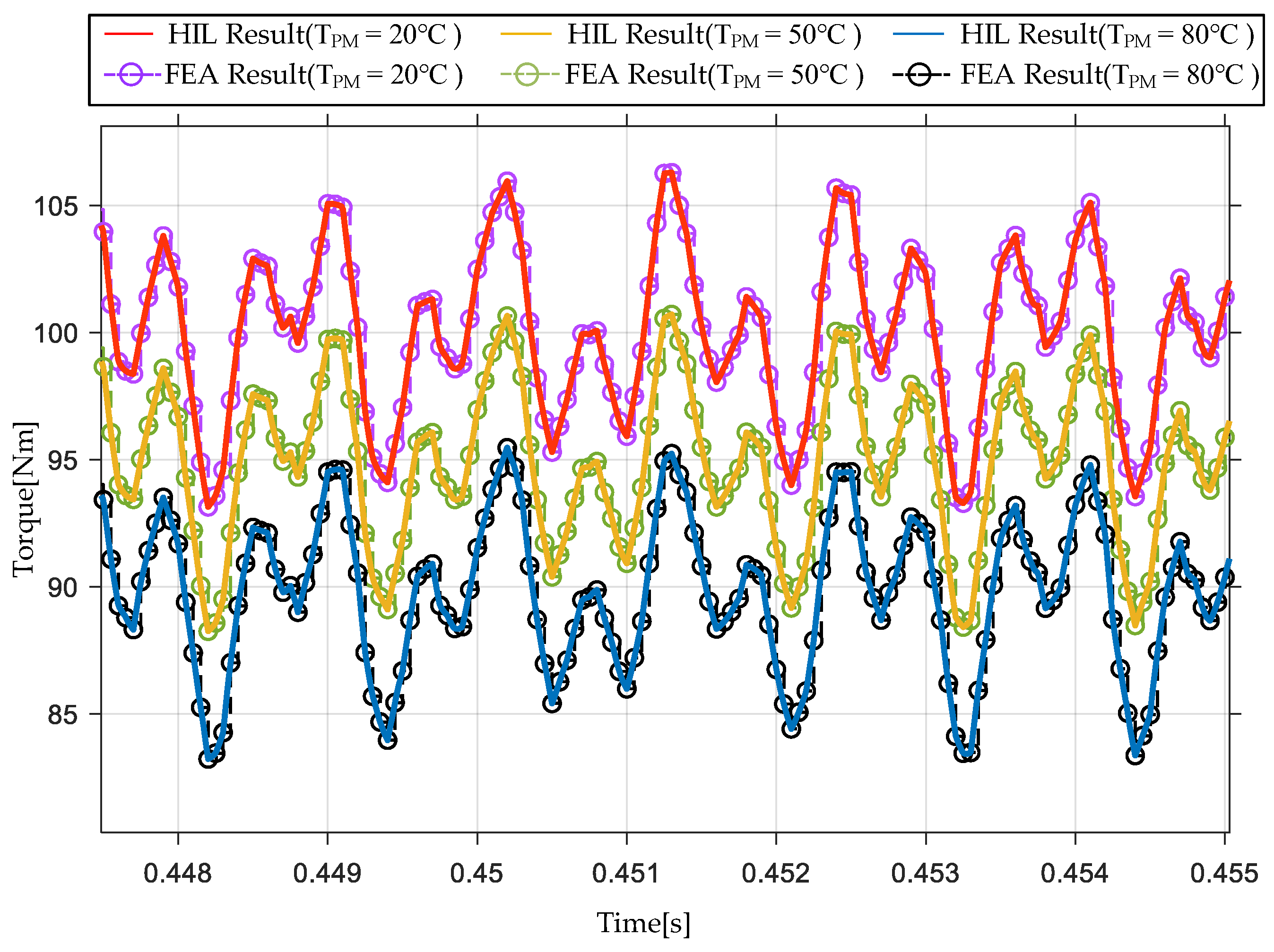
Figure 21 shows the HIL test results of the single operating condition. The operation conditions are as follows: the speed of 2000 RPM and the torque of 100 Nm. The winding temperature and the permanent magnet temperature are set through the host computer. The initial temperature state is set to and . Then and are set to verify the effect of the winding temperature effect. As can be seen in Figure 21, the effect of the winding temperature is not significant. For different winding temperature conditions, the motor torque varies at different rotor positions. However, the average torque is equal within one electrical period. This is due to the fact that the resistance voltage drop due to the temperature change of the windings is small and negligible compared to the motor back electromotive force. The impact of the permanent magnet temperature is more significant than that of the winding temperature. An increase in the temperature of the permanent magnet results in a notable decrease in the motor torque. This is due to the fact that the winding temperature only affects the winding resistance. As shown in Figure 9, Figure 10, Figure 11 and Figure 12, the permanent magnet temperature can have a significant effect on the bidirectional mapping relationship between the current and the flux-linkage, which directly affects the torque of the motor.

Figure 21.
Torque test results for different temperature conditions.
Figure 22 shows the comparison between the torque test results and the FEA results under different temperature conditions. It is similar to the results shown in Figure 19, and there is a good match between the torque test results and the FEA calculation results. This implies that the improved IPMSM model is capable of incorporating the effects of temperature factors into the HIL test model, which improves the applicability of the HIL test.
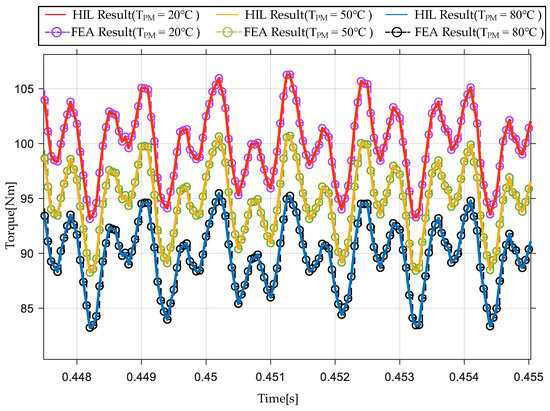
Figure 22.
Comparison of torque test results with FEA results at different temperature conditions.
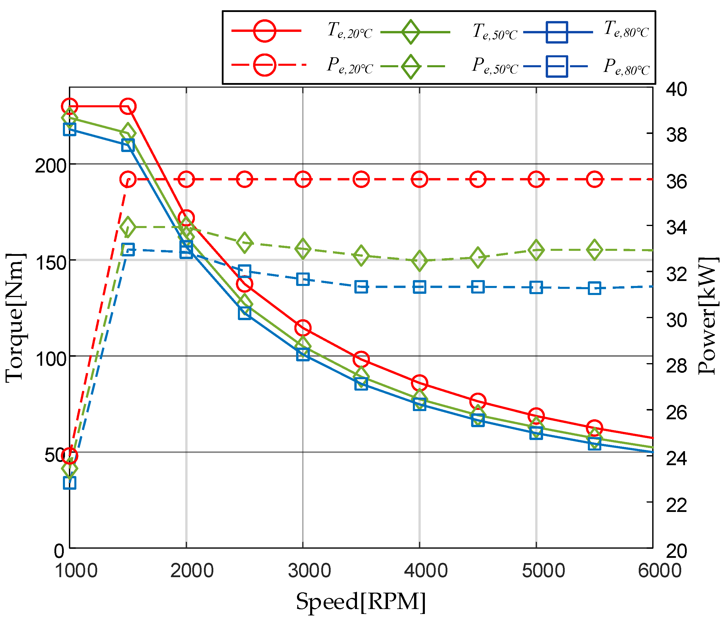
The speed-power characteristic of the IPMSM under test is shown in Figure 23. Since the effect of winding temperature on motor torque is insignificant, for the sake of simplicity, the external characteristic test is performed with the winding temperature set to be identical to the temperature of the permanent magnet. As previously discussed, the reduction in power is associated with the temperature-dependent behaviour of the torque. As shown in the figure, an increase in the temperature of the permanent magnet results in a corresponding decline in motor power.

Figure 23.
Torque and power test results for different temperature conditions.
4.4. Case 3: Validation of Iron Loss Effect
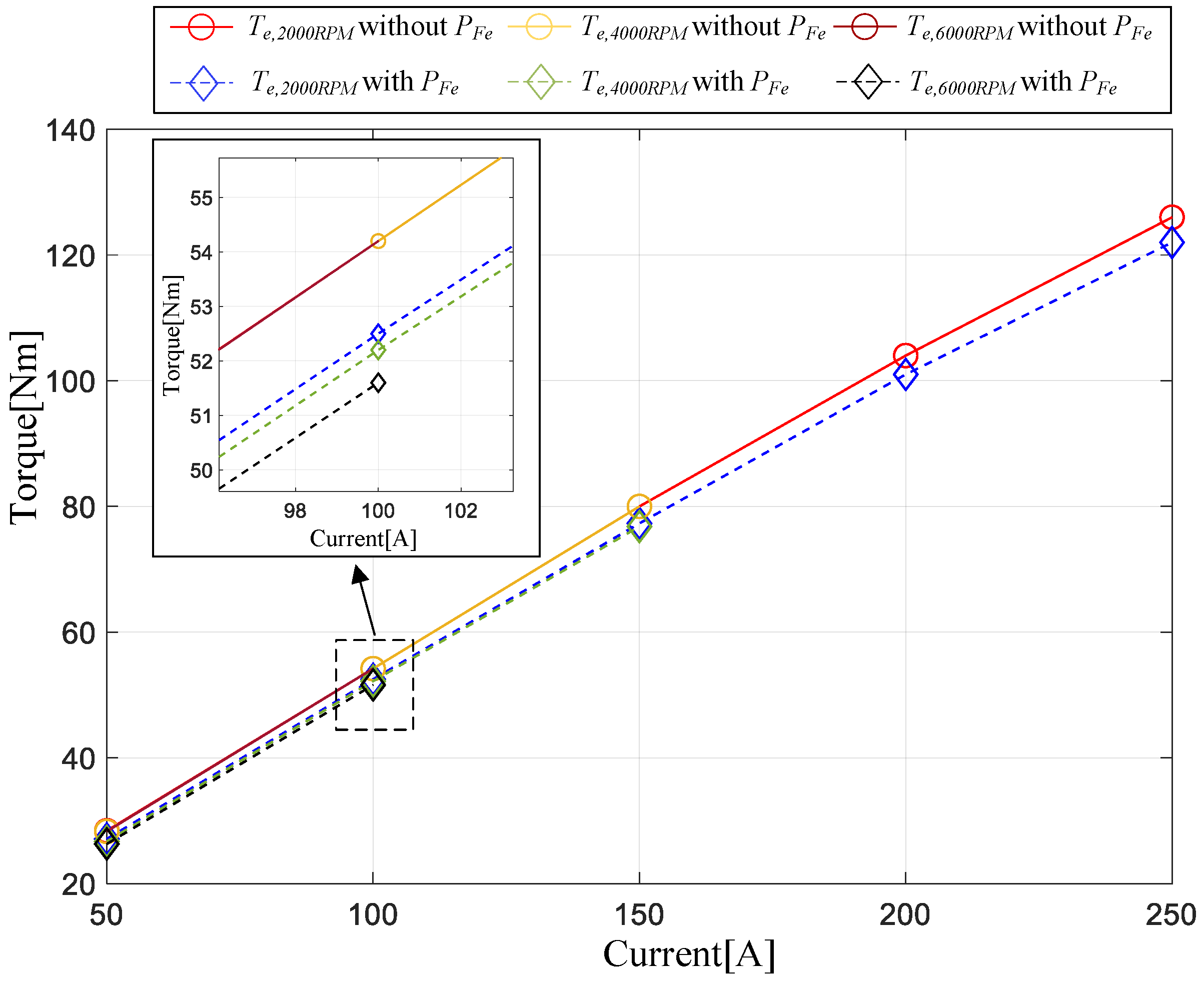
In Case 3, the constant current mode of the motor controller was employed for the purpose of verifying the effect of iron loss. The stator current amplitude was set in steps of 50 A, ranging from 50 A to 250 A, and the current phase angle (the angle between the current vector and the q-axis) was set to 50°. In order to eliminate the influence of the temperature factor, the stator winding temperature and the permanent magnet temperature were set at . The impact of the iron loss factor was evaluated by either activating or inactivating the iron loss current calculation module shown in Figure 17. Since iron loss is related to motor speed, the motor speed was set to 2000 RPM, 4000 RPM, and 6000 RPM for comparison of results.
Figure 24 shows the comparison of motor torque with and without considering the iron loss effect at different speed conditions. In Figure 24, the results at the current amplitude of 100 A are zoomed in locally to compare the results at different speeds. From the figure, it can be observed that identical motor torque can be achieved with the same stator current excitation for the specified speed condition when the iron loss effect is not taken into account. Nevertheless, when the iron loss effect is incorporated into the model, the identical current excitation does not yield the same torque. As the speed of the motor increases, there is a corresponding decrease in motor torque. This is due to the fact that when iron losses are taken into account, not all of the stator current flowing through the motor end acts as the conversion between electromechanical energy. As shown in Figure 14, a proportion of the stator current is consumed in the form of iron losses, and the iron loss current increases in correlation with the motor speed.

Figure 24.
Torque test results with and without the iron loss effect.
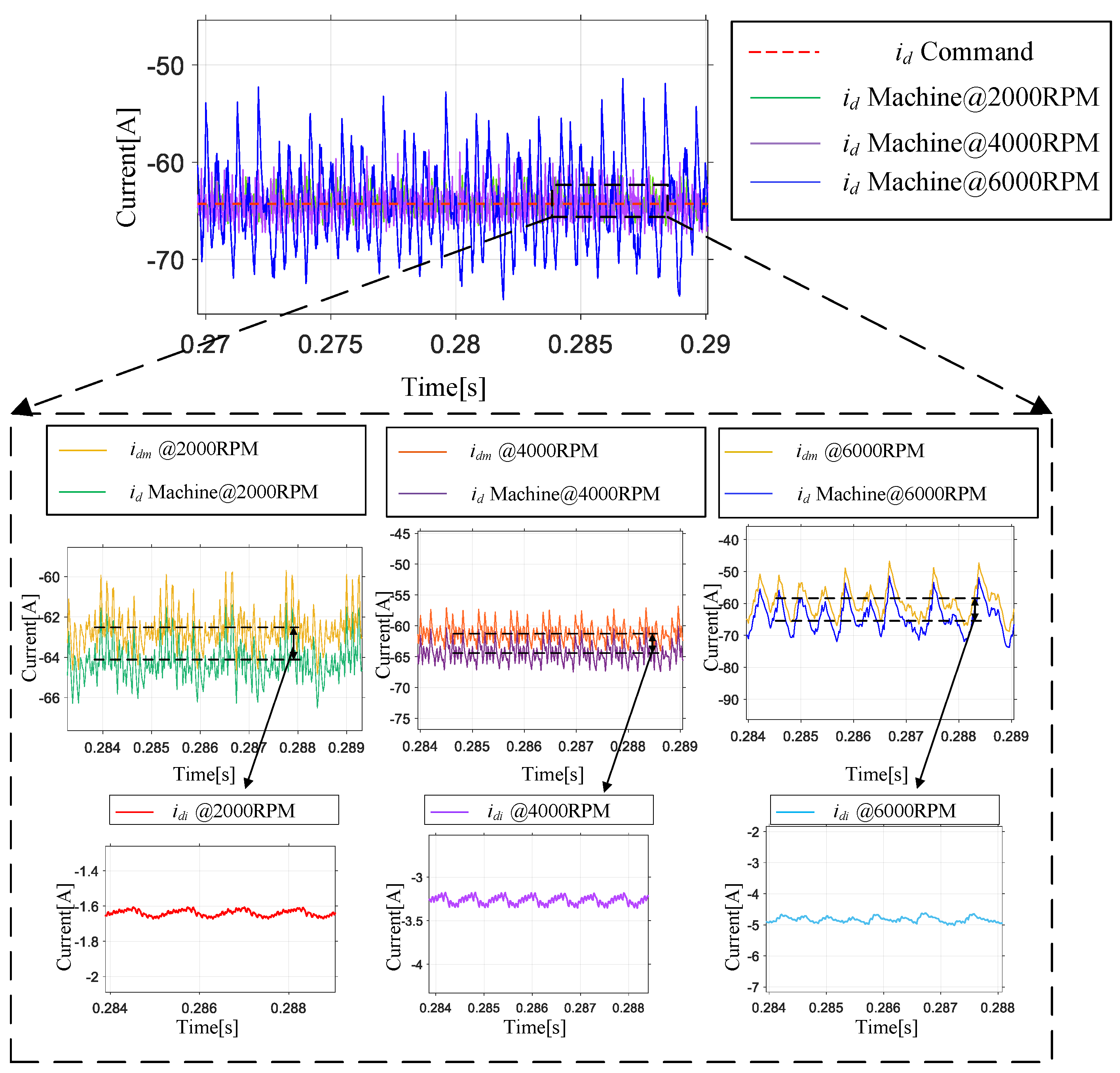
Figure 25 shows the current control results for different speed conditions considering the iron loss effect. For readability of the figure, only the results for d-axis currents are shown here. From the figure, it can be observed that while the current ripple exhibits a gradual growth in response to increasing motor speed, the d-axis total current remains capable of following the command. This is because the d-axis total current is sampled and negative feedback closed loop control is applied to it. However, as shown in the partially zoomed-in view of the dotted box, the iron loss current component and the magnetization current components show different variations for different speed conditions. The amplitude and percentage of the iron loss current component increase with the speed of the motor. Table 2 presents a summary of these test results.

Figure 25.
Current test results with iron loss effect ( and ).

Table 2.
Summary of iron loss test results.
5. Conclusions
This paper proposes an improved IPMSM nonlinear motor model which takes into account saturation, cross-coupling, spatial harmonics, temperature and iron loss effects. The proposed model provides an efficient and reliable approach for the evaluation of IPMSM operational performance. Moreover, it can serve as a foundation for the development of high-performance control algorithms, including those for torque ripple suppression, sensorless control, and other algorithms. The discrete-time form of the improved model is established directly. It can be straightforwardly incorporated into both MATLAB/Simulink environments and implemented on FPGA-based HIL test platforms. Three test cases are performed to evaluate the proposed nonlinear model. The effectiveness and feasibility of the proposed model are verified by HIL tests. The test results show that saturation, cross-coupling, spatial harmonics, iron loss, and temperature factors can be incorporated into the HIL test by the improved model, which improves the applicability of the HIL test.
In this paper, the motor data was calculated through a 2D FEA model without considering the effect of winding-end factors. In future work, the winding-end factors can be included in the analysis through a 3D FEA model. Furthermore, it may be beneficial to investigate additional model order reduction methods with a view to reducing the storage load of FPGAs.
Author Contributions
Conceptualization, Y.F. and J.L.; methodology, Y.F. and J.L.; software, Y.F. and G.Z.; validation, Y.F. and G.Z.; formal analysis, Y.F.; investigation, Y.F.; resources, J.L.; data curation, Y.F.; writing—original draft preparation, Y.F.; writing—review and editing, Y.F., G.Z. and J.L.; visualization, Y.F.; supervision, J.L.; project administration, J.L.; funding acquisition, J.L. All authors have read and agreed to the published version of the manuscript.
Funding
This research received no external funding.
Data Availability Statement
All the data are shown in the tables and figures of this paper.
Conflicts of Interest
The authors declare no conflict of interest.
Abbreviations
The following abbreviations are used in this manuscript:
| Terms | Units | Meaning |
| IPMSM | Interior permanent magnet synchronous motor | |
| FPGA | Field programmable gate array | |
| LuT | Look-up table | |
| FEA | Finite element analysis | |
| A | Stator current | |
| A | d- and q-axis stator current | |
| A | Iron loss current component | |
| A | Magnetization current component | |
| mH | d- and q-axis inductance | |
| Wb | d- and q-axis stator flux-linkage | |
| Wb | Permanent-magnet flux-linkage | |
| Number of pole pairs | ||
| V | d- and q-axis stator voltage | |
| rad/s | Electrical rotor speed | |
| RPM | Mechanical rotor speed | |
| rad | Electrical rotor position angle | |
| Nm | Electromagnetic torque | |
| Ω | Stator winding resistance | |
| Ω | Resistance at reference temperature | |
| 1/°C | Temperature coefficient of resistance | |
| °C | Reference temperature in FEA software | |
| °C | Temperature set for the stator winding in the IPMSM model | |
| °C | Temperature set for permanent magnet in the IPMSM model | |
| °C | Base value of temperature variance | |
| Ω | d- and q-axis iron loss resistence | |
| W | Total eddy current loss power | |
| W | Total hysteresis loss power | |
| W | d- and q-axis total iron loss power | |
| W | d- and q-axis eddy current loss power | |
| W | d- and q-axis hysteresis loss power | |
| d-axis flux-linkage function considering saturation and cross-coupling effects | ||
| q-axis flux-linkage function considering saturation and cross-coupling effects | ||
| d-axis current function considering saturation and cross-coupling effects | ||
| q-axis current function with considering saturation and cross-coupling effects | ||
| d-axis flux-linkage function considering saturation, cross-coupling and spatial harmonics effects | ||
| q-axis flux-linkage function considering saturation, cross-coupling and spatial harmonics effects | ||
| d-axis current function considering saturation, cross-coupling and spatial harmonics effects | ||
| q-axis current function considering saturation, cross-coupling and spatial harmonics effects | ||
| d-axis flux-linkage function considering saturation, cross-coupling, spatial harmonics and temperature effects | ||
| q-axis flux-linkage function considering saturation, cross-coupling, spatial harmonics and temperature effects |
Appendix A
Details of Current Shift Equation
During the research process, the relevant data were analyzed, and it was found that the temperature factor influences the current shift throughout the dq-axis current plane. Figure A1 and Table A1 show the relevant data. Based on these data, two key observations were found. Firstly, an approximate linear relationship was observed between the shifts in the d- and q-axis currents and temperature. Secondly, for different d- and q-axis flux-linkage values, the current shift’s base value was different and varied with the flux-linkage value. These observations led to the formulation of Equations (A1) and (A2). The temperature-dependent scaling operation in equations reflects the linear variation characteristic observed above.
where and can be calculated by the following equation.
where the content indicates that the base value of the current shift is correlated with the flux-linkage, reflecting the second characteristic mentioned above. In (A3) and (A4), the temperature represented by x °C can be chosen arbitrarily due to the linear characteristic. Correspondingly, can be calculated as follows.
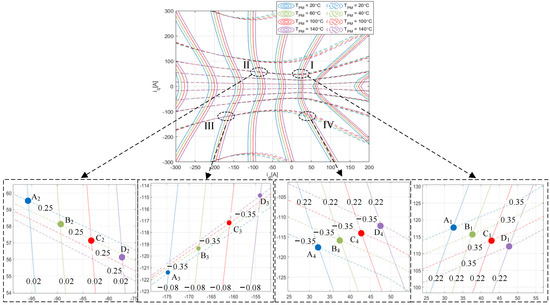
Figure A1.
The flux-linkage mapping at different PM temperatures.
Figure A1.
The flux-linkage mapping at different PM temperatures.
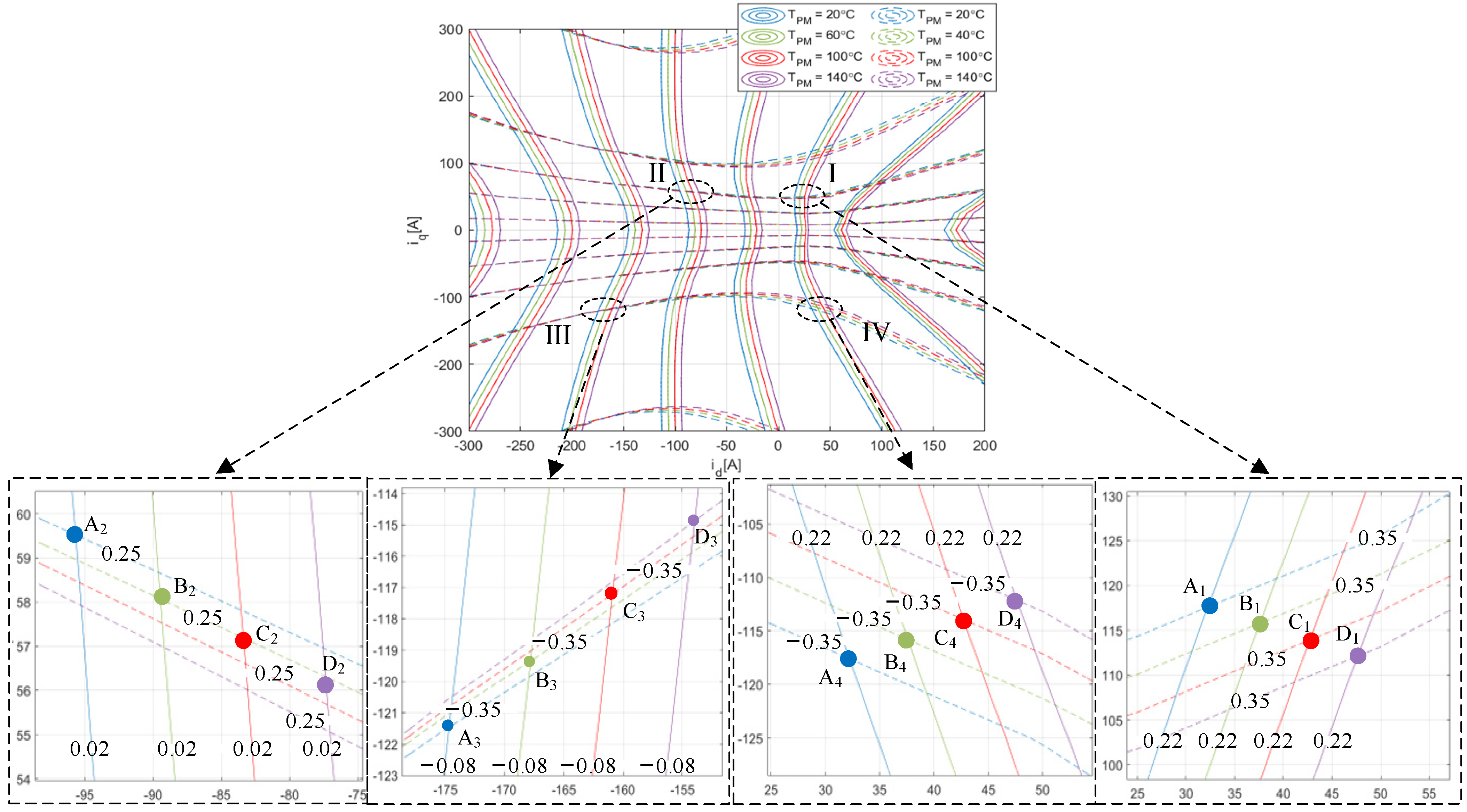
In Figure A1, the solid line represents the daxis fluxlinkage, and the dashed line represents the qaxis fluxlinkage.

Table A1.
Summary of current data.
Table A1.
Summary of current data.
| Temperature [°C] | Flux-Linkage [Wb] | Current [A] | d-axis Current Shift [A] | q-axis Current Shif [A] | Temperature Difference [°C] | ||
|---|---|---|---|---|---|---|---|
| I | A1 | 20 | (0.22,0.35) | (32.5,117.6) | / | / | / |
| B1 | 60 | (0.22,0.35) | (37.6,115.8) | 5.1 | −1.8 | 40 | |
| C1 | 100 | (0.22,0.35) | (42.7,113.9) | 10.2 | −3.7 | 80 | |
| D1 | 140 | (0.22,0.35) | (47.7,112.2) | 15.2 | −5.4 | 120 | |
| II | A2 | 20 | (0.02,0.25) | (−95.7,59.3) | / | / | / |
| B2 | 60 | (0.02,0.25) | (−89.5,57.9) | 6.2 | −1.4 | 40 | |
| C2 | 100 | (0.02,0.25) | (−83.2,56.4) | 12.5 | −2.9 | 80 | |
| D2 | 140 | (0.02,0.25) | (−77,55) | 18.7 | −4.3 | 120 | |
| III | A3 | 20 | (−0.08,−0.35) | (−174.4,−121.5) | / | / | / |
| B3 | 60 | (−0.08,−0.35) | (−167.8,−119.4) | 6.6 | 2.1 | 40 | |
| C3 | 100 | (−0.08,−0.35) | (−160.9,−117.2) | 13.5 | 4.3 | 80 | |
| D3 | 140 | (−0.08,−0.35) | (−154.1,−114.9) | 20.3 | 6.6 | 120 | |
| IV | A4 | 20 | (0.22,−0.35) | (32.2,−117.6) | / | / | / |
| B4 | 60 | (0.22,−0.35) | (37.6,−115.8) | 5.4 | 1.8 | 40 | |
| C4 | 100 | (0.22,−0.35) | (42.8,−113.9) | 10.6 | 3.7 | 80 | |
| D4 | 140 | (0.22,−0.35) | (47.9,−112.2) | 15.7 | 5.4 | 120 |
References
- Arias, N.B.; Hashemi, S.; Andersen, P.B.; Træholt, C.; Romero, R. Distribution System Services Provided by Electric Vehicles: Recent Status, Challenges, and Future Prospects. IEEE Trans. Intell. Transp. Syst. 2019, 20, 4277–4296. [Google Scholar] [CrossRef]
- Agamloh, E.; von Jouanne, A.; Yokochi, A. An Overview of Electric Machine Trends in Modern Electric Vehicles. Machines 2020, 8, 20. [Google Scholar] [CrossRef]
- Alibeik, M.; dos Santos, E.C. High-Torque Electric Machines: State of the Art and Comparison. Machines 2022, 10, 636. [Google Scholar] [CrossRef]
- Pellegrino, G.; Vagati, A.; Guglielmi, P.; Boazzo, B. Performance Comparison between Surface-Mounted and Interior PM Motor Drives for Electric Vehicle Application. IEEE Trans. Ind. Electron. 2012, 59, 803–811. [Google Scholar] [CrossRef]
- Yang, Y.; Castano, S.M.; Yang, R.; Kasprzak, M.; Bilgin, B.; Sathyan, A.; Dadkhah, H.; Emadi, A. Design and Comparison of Interior Permanent Magnet Motor Topologies for Traction Applications. IEEE Trans. Transp. Electrif. 2017, 3, 86–97. [Google Scholar] [CrossRef]
- Zhu, Z.Q.; Chu, W.Q.; Guan, Y. Quantitative Comparison of Electromagnetic Performance of Electrical Machines for Hevs/Evs. CES Trans. Electr. Mach. Syst. 2017, 1, 37–47. [Google Scholar] [CrossRef]
- Sahu, A.K.; Haddad, R.Z.; Al-Ani, D.; Bilgin, B. Thermomechanical Rotor Fatigue of an Interior Permanent Magnet Synchronous Motor. Machines 2024, 12, 158. [Google Scholar] [CrossRef]
- Sul, S.-K. Basic Structure and Modeling of Electric Machines and Power Converters. In Control of Electric Machine Drive Systems; Wiley: Hoboken, NJ, USA, 2010. [Google Scholar]
- Zhu, Z.Q.; Wu, X.M. Fundamental Model-Based Sensorless Control. In Sensorless Control of Permanent Magnet Synchronous Machine Drives; Wiley: Hoboken, NJ, USA, 2023. [Google Scholar]
- Dufour, C.; Belanger, J.; Abourida, S.; Lapointe, V. Fpga-Based Real-Time Simulation of Finite-Element Analysis Permanent Magnet Synchronous Machine Drives. In Proceedings of the 2007 IEEE Power Electronics Specialists Conference, Orlando, FL, USA, 17–21 June 2007. [Google Scholar]
- Xu, F.; Dinavahi, V.; Xu, X. Hybrid Analytical Model of Switched Reluctance Machine for Real-Time Hardware-in-the-Loop Simulation. IET Electr. Power Appl. 2017, 11, 1114–1123. [Google Scholar] [CrossRef]
- Bastos, R.F.; Silva, F.B.; Aguiar, C.R.; Fuzato, G.; Machado, R.Q. Low-Cost Hardware-in-the-Loop for Real-Time Simulation of Electric Machines and Electric Drive. IET Electr. Power Appl. 2020, 14, 1679–1685. [Google Scholar] [CrossRef]
- Stumberger, G.; Polajzer, B.; Stumberger, B.; Toman, M.; Dolinar, D. Evaluation of Experimental Methods for Determining the Magnetically Nonlinear Characteristics of Electromagnetic Devices. IEEE Trans. Magn. 2005, 41, 4030–4032. [Google Scholar] [CrossRef]
- Chen, X.; Wang, J.; Sen, B.; Lazari, P.; Sun, T. A High-Fidelity and Computationally Efficient Model for Interior Permanent-Magnet Machines Considering the Magnetic Saturation, Spatial Harmonics, and Iron Loss Effect. IEEE Trans. Ind. Electron. 2015, 62, 4044–4055. [Google Scholar] [CrossRef]
- Dufour, C.; Abourida, S.; Belanger, J. Real-Time Simulation of Permanent Magnet Motor Drive on Fpga Chip for High-Bandwidth Controller Tests and Validation. In Proceedings of the 2006 IEEE International Symposium on Industrial Electronics, Montreal, QC, Canada, 9–13 July 2006. [Google Scholar]
- Florin, P.P.; Mircea, R.; Raul, N.; Martis, C.; Adrian-Cornel, P. Real-Time Model in the Loop Analysis of Pmsm for Electric Power Steering System Based on Fpga Implementation. In Proceedings of the 2018 International Symposium on Power Electronics, Electrical Drives, Automation and Motion (SPEEDAM), Amalfi, Italy, 20–22 June 2018. [Google Scholar]
- Janouš, Š.; Talla, J.; Košan, T.; Peroutka, Z. Fpga-Based Real-Time Hil Simulator of Permanent Magnet Synchronous Motor Drive. In Proceedings of the 2021 IEEE 19th International Power Electronics and Motion Control Conference (PEMC), Gliwice, Poland, 25–29 April 2021. [Google Scholar]
- Hu, D.; Alsmadi, Y.M.; Xu, L. High-Fidelity Nonlinear IPM Modeling Based on Measured Stator Winding Flux Linkage. IEEE Trans. Ind. Appl. 2015, 51, 3012–3019. [Google Scholar] [CrossRef]
- Quéval, L.; Ohsaki, H. Nonlinear Abc-Model for Electrical Machines Using N-D Lookup Tables. IEEE Trans. Energy Convers. 2015, 30, 316–322. [Google Scholar] [CrossRef]
- Luo, G.; Zhang, R.; Chen, Z.; Tu, W.; Zhang, S.; Kennel, R. A Novel Nonlinear Modeling Method for Permanent-Magnet Synchronous Motors. IEEE Trans. Ind. Electron. 2016, 63, 6490–6498. [Google Scholar] [CrossRef]
- Xu, L.; Xu, X.; Lipo, T.A.; Novotny, D.W. Vector Control of a Synchronous Reluctance Motor Including Saturation and Iron Loss. IEEE Trans. Ind. Appl. 1991, 27, 977–985. [Google Scholar] [CrossRef]
- Morimoto, S.; Tong, Y.; Takeda, Y.; Hirasa, T. Loss Minimization Control of Permanent Magnet Synchronous Motor Drives. IEEE Trans. Ind. Electron. 1994, 41, 511–517. [Google Scholar] [CrossRef]
- Dück, P.; Ponick, B. A Novel Iron-Loss-Model for Permanent Magnet Synchronous Machines in Traction Applications. In Proceedings of the 2016 International Conference on Electrical Systems for Aircraft, Railway, Ship Propulsion and Road Vehicles & International Transportation Electrification Conference (ESARS-ITEC), Toulouse, France, 2–4 November 2016. [Google Scholar]
- Urasaki, N.; Senjyu, T.; Uezato, K. A Novel Calculation Method for Iron Loss Resistance Suitable in Modeling Permanent-Magnet Synchronous Motors. IEEE Trans. Energy Convers. 2003, 18, 41–47. [Google Scholar] [CrossRef]
- Li, S.; Han, D.; Sarlioglu, B. Modeling of Interior Permanent Magnet Machine Considering Saturation, Cross Coupling, Spatial Harmonics, and Temperature Effects. IEEE Trans. Transp. Electrif. 2017, 3, 682–693. [Google Scholar] [CrossRef]
- Cai, H.; Hu, D. On Pmsm Model Fidelity and Its Implementation in Simulation. In Proceedings of the 2018 IEEE Energy Conversion Congress and Exposition (ECCE), Portland, OR, USA, 23–27 September 2018. [Google Scholar]
- Di Tommaso, A.O.; Miceli, R.; Nevoloso, C.; Scaglione, G.; Schettino, G. Improved High-Fidelity IPMSM mathematical model Including Saturation, Cross-Coupling, Torque Ripple and Iron Loss effects. In Proceedings of the 2022 International Conference on Electrical Machines (ICEM), Valencia, Spain, 5–8 September 2022; pp. 21–27. [Google Scholar]
- Wang, M. A Novel Mathematical Nonlinear PMSM Realization Method for Electric Machine Emulator. IEEE J. Emerg. Sel. Top. Power Electron. 2022, 10, 4171–4181. [Google Scholar] [CrossRef]
- Sintered Neodymium-Iron-Boron Magnets N38UH. Available online: https://www.arnoldmagnetics.com/wp-content/uploads/2017/11/N38UH-151021.pdf (accessed on 12 July 2016).
Disclaimer/Publisher’s Note: The statements, opinions and data contained in all publications are solely those of the individual author(s) and contributor(s) and not of MDPI and/or the editor(s). MDPI and/or the editor(s) disclaim responsibility for any injury to people or property resulting from any ideas, methods, instructions or products referred to in the content. |
© 2025 by the authors. Licensee MDPI, Basel, Switzerland. This article is an open access article distributed under the terms and conditions of the Creative Commons Attribution (CC BY) license (https://creativecommons.org/licenses/by/4.0/).

