A Real-Time Demanded Current Observation-Based Sliding Mode Control of Permanent Magnet Synchronous Motors

Abstract

To improve the dynamic and steady-state performance of permanent magnet synchronous motors (PMSM), this paper proposes a real-time demanded current observation based sliding mode control strategy. Firstly, based on the mechanism between motor speed and current, a real-time demanded current observer is proposed, which can obtain the demanded current based on the motor speed. Secondly, the demanded current is directly used to calibrate the q-axis current reference in real-time, which can update the current reference value faster than the sliding mode controller. Due to the real-time demanded current feedforward, the anti-interference performance of the PMSM under the proposed control is improved effectively. Compared with the conventional sliding mode control, the proposed control has a better dynamic and steady-state performance. Finally, the effectiveness of the proposed control has been verified through simulation and experiments.

1. Introduction

With the global new energy program being vigorously implemented, the application scope of motors has been expanding continuously. Permanent magnet synchronous motors (PMSM), owing to their remarkable features such as high efficiency, compact size, and a host of other advantages, have found extensive applications in rail transit, industrial transmission, and energy vehicles (EVs) [1]. The control technology of PMSM serves as the core element to ensure their efficient and stable operation. Nevertheless, the PMSM is an intrinsically nonlinear complex system [2]. Each equation within the system exhibits a pronounced coupling phenomenon, and parameters are subject to change under certain conditions, such as in the presence of current coupling and load interference. When conventional PI control is employed, the required control output tends to fluctuate within a specific range [3]. Moreover, due to the strong dependence of the PI control method on the accuracy of the system model, it is highly sensitive to uncertain interferences and parameters. This sensitivity may have a negative impact on the expected output, thereby causing issues in the control system [4]. Consequently, to surmount the limitations of conventional PI control, it is imperative to develop advanced nonlinear control strategies and apply them to PMSM speed control systems. Examples of such strategies include active disturbance rejection control [5], model predictive control [6,7], fuzzy control [8,9], adaptive control [10,11], neural network control [12], and sliding mode control (SMC) [13,14]. These methods enhance the performance of the PMSM control system from diverse perspectives. Among them, SMC has emerged as a focal point of research due to its high precision control capabilities, robust nature, and relatively straightforward control algorithm [15]. In conventional SMC, the constant law has limitations in rapidly converging systematic errors. To overcome this issue, Hu et al. [16] incorporated a state variable into the constant law to improve the system’s response. Nevertheless, this conventional SMRL still struggles to effectively balance response speed and jitter. In [17], a reaching Law (ATSMRL) was proposed and applied to SMC, ATSMRL has the ability to reduce the computational complexity of control, enable flexible acceleration of convergence, and enhance system stability. In [18], an enhanced SMC was devised based on a new SMRL, integrating system variables, bounded exponential function, and switching gain; this method can expedite the system’s response and alleviate jitter. When the motor suffers from load disturbances, the load will influence the performance of SMC, making it difficult to effectively eliminate the impact of the disturbance. Research has indicated that the utilization of observers can reduce the impact of load disturbances. In [19], on the foundation of the constant law, NCRL was designed by integrating exponential function and piecewise function, it was proven that the initial state of the system does not affect the convergence speed, subsequently, an optimized observer was designed taking into account external load disturbances. This approach can accelerate the response while reducing output jitter and enhancing the anti-interference ability. In [20], a new reaching law (NRL) was designed by introducing system variables and switching gain terms into the exponential reaching law. The SMC design based on NRL can improve the system’s convergence speed. Since large switching gains can lead to jitter, an observer (ESMDO) was designed, ESMDO conducts feedforward compensation on SMC, thus improving system robustness and reducing jitter. In [21], ESO was designed based on current coupling and external interference, and combined with SMC, which not only achieved current decoupling but also improved the robustness of the system. In addition, research on composite control that combines multiple methods has also been carried out. In [22], SMC was developed through the utilization of an optimized neural network algorithm, and this approach is capable of enhancing the control accuracy via the optimization of control parameters.

In an attempt to enhance the dynamic and steady-state performance of SMC, this paper proposes a sliding mode control motor speed based on real time demand current observation. The main work is summarized as follows;

(1)

Designed a SMC based on exponential reaching law.

(2)

A real-time demand current observer was designed to observe q-axis current disturbances and compensate for q-axis current, and combined with SMC, called SMC-ESO. This not only improves the performance of SMC but also demonstrates some of its characteristics.

(3)

Experiments have been conducted under various disturbance conditions, all of which indicate that SMC-ESO has better control performance.

2. Mathematical Modeling of PMSM

The mathematical model of PMSM within the rotating coordinate system is presented as follows:

$${\displaystyle \frac{d{i}_d}{dt}}={\displaystyle \frac{1}{L_d}}{u}_d-{\displaystyle \frac{R_s}{L_d}}{i}_d+{\displaystyle \frac{\omega }{L_d}}{\psi }_q.$$

(1)

$${\displaystyle \frac{d{i}_q}{dt}}={\displaystyle \frac{1}{L_q}}{u}_q-{\displaystyle \frac{R_s}{L_q}}{i}_q-{\displaystyle \frac{\omega }{L_d}}{\psi }_d.$$

(2)

The mechanical equations of motion are as follows:

$${\displaystyle \frac{d\omega }{dt}}={\displaystyle \frac{p}{J}}{T}_{\mathrm{e}}-{\displaystyle \frac{p}{J}}{T}_{\mathrm{L}}-{\displaystyle \frac{B\omega }{J}}.$$

(3)

For surface-mounted PMSM, there is L_d = L_q = L, so there is an electromagnetic torque equation as follows:

$$T_{\mathrm{e}}={\displaystyle \frac{3}{2}}p\left[{\psi }_{\mathrm{f}}{i}_{\mathrm{q}}+\left(L_{\mathrm{d}}-L_{\mathrm{q}}\right)i_{\mathrm{q}}{i}_{\mathrm{d}}\right]={\displaystyle \frac{3}{2}}p{\psi }_{\mathrm{f}}{i}_{\mathrm{q}},$$

(4)

where U_d and U_q represent stator d and q-axis voltages, respectively; i_d and i_q are stator d and q-axis currents, respectively; R_s is stator resistance; L_d and L_q stand for stator d and q-axis inductances, respectively; ω is motor speed; ψ_f is the permanent magnet chain; ψ_d and ψ_q are stator d and q-axis chains, respectively; T_e is the electromagnetic torque; p is the number of pole pairs; J is the rotational moment of inertia; T_L is the load torque; d is the differential operator; B is the damping coefficient.

3. Design of Speed Controller

3.1. Design of Sliding Mode Controller

SMC is a variable structure control that is different from PI and is actually a nonlinear control. A motor control system is used to design the SMC.

Designing sliding mode control requires two steps. Firstly, the system slip mold surface is designed as follows:

$$s=c{x}_1+x_2,$$

(5)

where c is a constant.

Second, the design of the reaching law. The exponential reaching law can effectively reduce sliding mode jitter, and the output calculation is relatively simple and intuitive. It adopts the following form [19]:

$$\dot{s}=-\epsilon \mathrm{sgn}(s)-ks,$$

(6)

where s denotes the deviation between the estimated value and the actual value, sgn () is a sign function εsgn() represents a constant value reaching term, ks represents an exponential reaching term, both ε and k are constants with values greater than zero.

The system state equation of the PMSM is taken as:

$$\left\{\begin{array}{l}\hfill x_1={\omega }^{\ast }-\omega \hfill \\ x_2={\dot{x}}_1=-\dot{\omega }\hfill \end{array}\right.,$$

(7)

where ω—the reference speed,

ω*—the actual speed.

Combining (7) and (9) gives,

$$\left\{\begin{array}{l}{\dot{x}}_1=-\dot{\omega }=-{\displaystyle \frac{1}{J}}\left({\displaystyle \frac{3}{2}}{p}^2{\mathsf{\Psi }}_{\mathrm{f}}{i}_{\mathrm{q}}-p{T}_{\mathrm{L}}-B\omega \right)\hfill \\ \hfill {\dot{x}}_2=-\ddot{\omega }=-{\displaystyle \frac{3p^2}{2J}}{\mathsf{\Psi }}_{\mathrm{f}}{\dot{i}}_{\mathrm{q}}+{\displaystyle \frac{B\dot{\omega }}{J}}=-{\displaystyle \frac{3p^2}{2J}}{\mathsf{\Psi }}_{\mathrm{f}}{\dot{i}}_{\mathrm{q}}-{\displaystyle \frac{B}{J}}{x}_2\hfill \end{array},\right.$$

(8)

let A = 3p2ψ_f/2J, D = −B/J. The state equation of the system can be formulated as follows:

$$\left(\begin{array}{l}{\dot{x}}_1\\ {\dot{x}}_2\end{array}\right)=\left(\begin{array}{cc}0& 1\\ 0& D\end{array}\right)\left(\begin{array}{l}{x}_1\\ x_2\end{array}\right)+\left(\begin{array}{l}0\\ -A\end{array}\right){\dot{i}}_{\mathrm{q}}.$$

(9)

The partial derivative of s yields the following result:

$$\dot{s}=c{\dot{x}}_1+{\dot{x}}_2=(c+D)x_2-A{\dot{i}}_{\mathrm{q}}.$$

(10)

For obtaining the control variable, the exponential reaching law in the reaching law with restricted s form is chosen, the set of simultaneous equations, namely Equations (6), (10) and (11) can be represented in the following form:

$$-\epsilon sgn(s)-ks=(c+D)x_2-A{\dot{i}}_{\mathrm{q}},$$

(11)

the expression for the control quantity i_q is obtained from Equation (11) as follows:

$$i_q={\displaystyle \frac{1}{A}}\int ((c+D)x_2+\epsilon sgn(s)+ks)dt.$$

(12)

The Lyapunov function is selected as V = 0.5 s², according to the Lyapunov stability theory, when s ≠ 0, for the stability of SMC, the following conditions must be satisfied.

$$s\dot{s}<0,$$

(13)

from (6) and (13), the following can be obtained:

$$s\dot{s}=s(-\epsilon sgn(s)-ks),$$

(14)

where ε and k are constants greater than zero, ensuring that s is dissimilar to $\dot{s}$ and satisfies the stability condition, proving that the system under convergence law smooth mode control is stable.

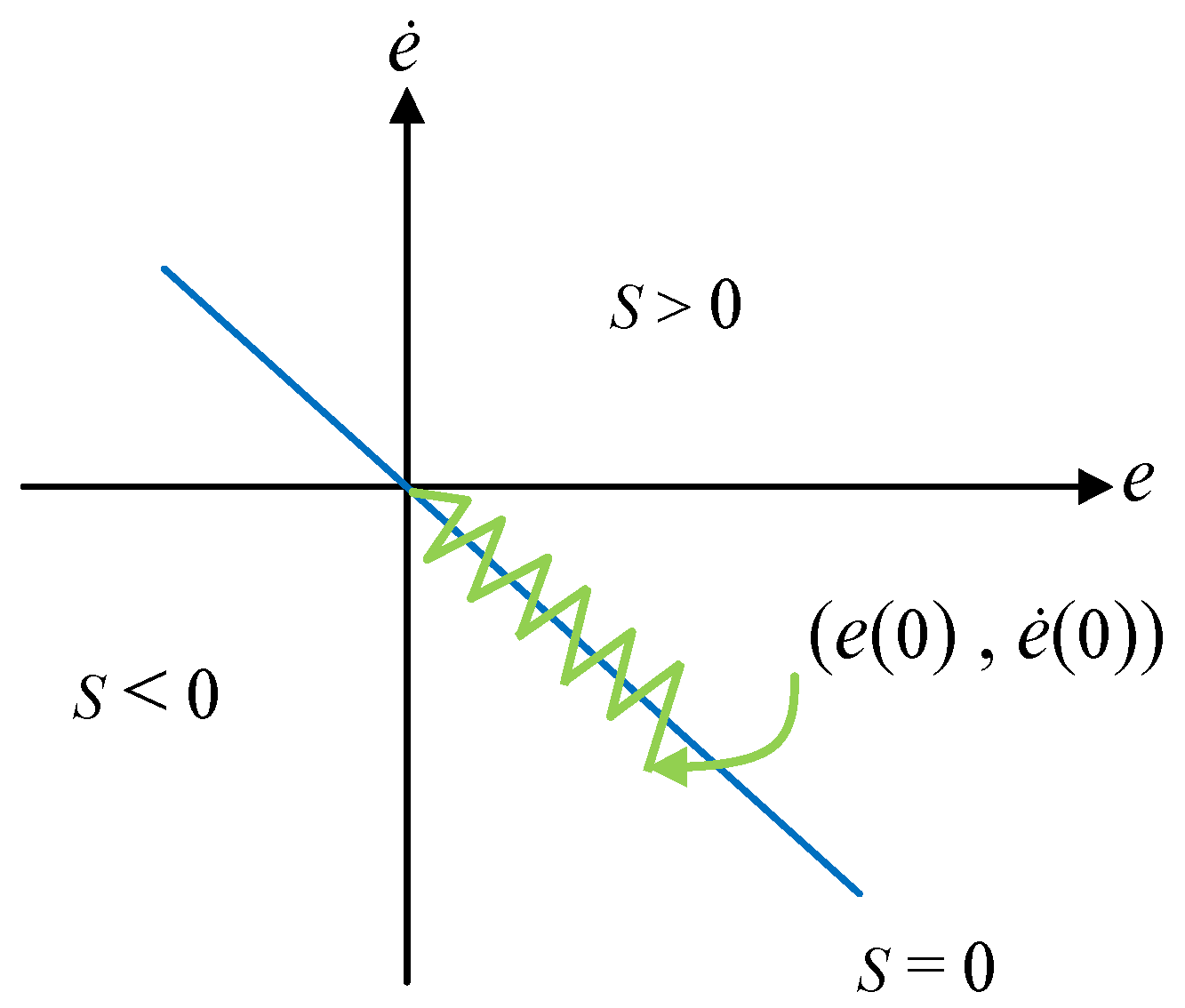
The motion trajectory of SMC guidance system closely follows a predesigned sliding surface. When the state trajectory of the variables essential to the system reaches this surface, the system demonstrates remarkable robustness. The motion trajectory of SMC is shown in Figure 1, the trajectory of the moving point within the system can be comprehensively classified into two primary stages. In the initial stage, the system initiates an approaching motion, starting from its current state, it gradually converges towards the predesigned surface. This approaching motion is crucial as it sets the stage for the subsequent behavior of the system. In the second stage, once the system has reached the predesigned surface, it engages in a reciprocating motion, the motion trajectory begins to closely align with the surface defined by s = 0. At this stage, the movement is characterized by high frequency oscillations accompanied by small amplitude jitter.

Figure 1. Motion trajectory of SMC.

3.2. Design of Extended State Observer

The extended state observer (ESO) serves as the core component of ADRC. It has the ability to observe the essential state variables and their derivatives, and can estimate system disturbances and implement corresponding compensation measures. In the theory of ADRC, the state error feedback control law (SEF) is employed to integrate the system state information with the observation output of ESO. Eventually, through the combination with disturbance compensation, a new control quantity for the system is formed. This integrated approach effectively enhances the system’s ability to handle uncertainties and disturbances, thereby improving the overall control performance. ESO and SEF can be expressed as follows:

The models of ESO and SEF are Equations (15) and (16), respectively:

$$\left\{\begin{array}{l}e=z_1-y\hfill \\ {\dot{z}}_1=z_2-{\beta }_1{f}_{al}\left(e,\alpha ,\delta \right)+b_{0}u(t)\hfill \\ {\dot{z}}_2=-{\beta }_2{f}_{al}\left(e,\alpha ,\delta \right)\hfill \end{array}\right.,$$

(15)

$$u(t)=u_0(t)-z_2/b_0.$$

(16)

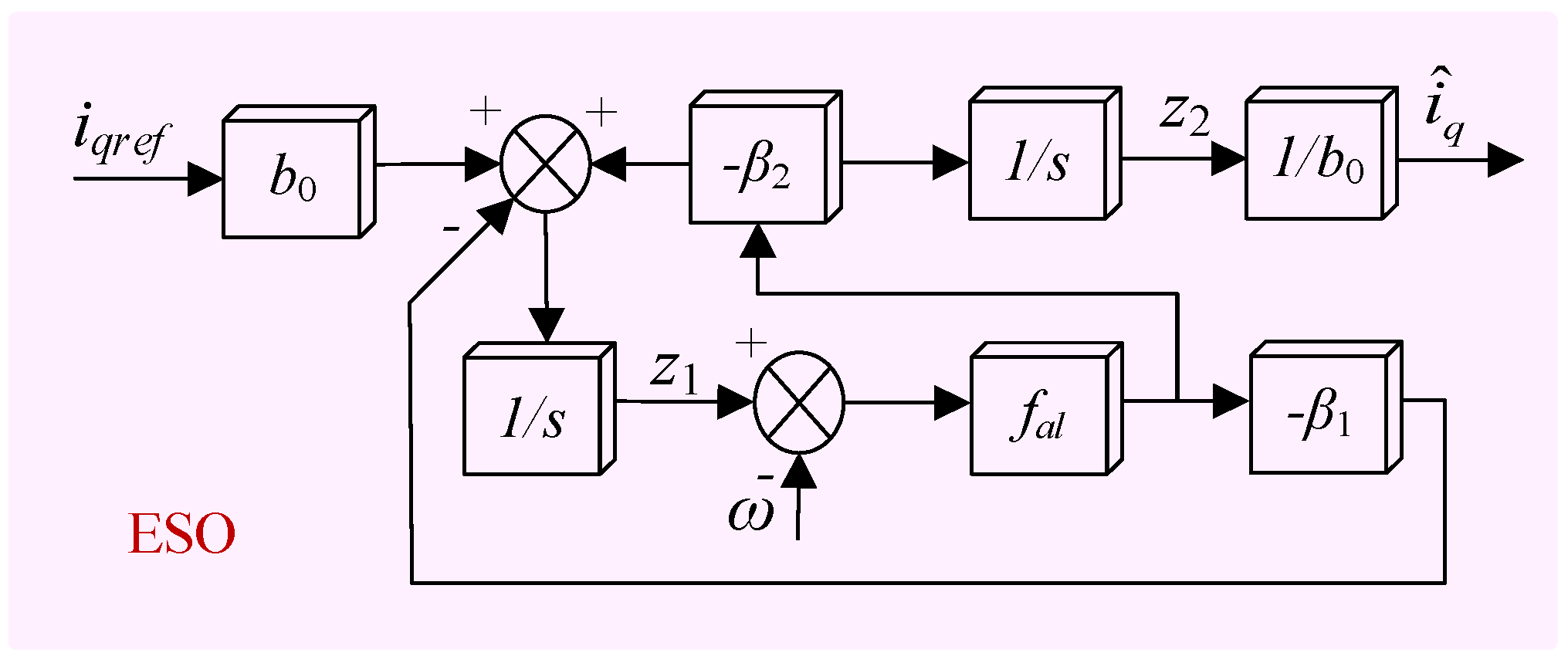
In the above ESO and SEF expressions, e is the error, y is the output signal of the controlled object, z₁, z₂ are the state variables of ESO, of which z₁ serves as the tracking signal for the output signal y, and z₂ is the observation of the total disturbance, α is the tracking factor; δ is the filtering factor, β₁ and β₂ are the ESO output error correction gains, b₀ is the compensation factor, which is used for the compensation of the external and internal disturbance, u₀ is the signal before compensation, f_al is the optimal control function, and the f_al function is essentially the compensation of “large error, small gain; small error, large gain” [22]. The expression for f_al is as follows:

$$f_{al}(e,\alpha ,\delta )=\left\{\begin{array}{l}|e{|}^{\alpha }\mathrm{sgn}(e),|e|>\delta \hfill \\ {\displaystyle \frac{e}{{\delta }^{1-\alpha }}},\left|e\right|<\delta \hfill \end{array}\right.,$$

(17)

in this equation, sgn is the sign function.

In order to control the motor’s given speed more accurately, ESO is designed for closed-loop control of the speed. According to (4) and (5), the motor speed output state equations are obtained as follows:

$${\displaystyle \frac{d\omega }{dt}}={\displaystyle \frac{3p^2{\psi }_{\mathrm{f}}}{2J}}{i}_q-{\displaystyle \frac{p}{J}}{T}_{\mathrm{L}}-{\displaystyle \frac{B\omega }{J}},$$

(18)

where (pT_L + Bω)/J is the system disturbance quantity, and let it be z₂, the disturbance observation current can be obtained as follows:

$${\widehat{i}}_q=z_2/b_0.$$

(19)

Designing the ESO, taking the actual output current i_qref as the control quantity u(t), and making the output current of SMC be i_q^*, the ESO expression can be introduced by combining (16) and (17) as:

$$\left\{\begin{array}{l}e=z_1-\omega \hfill \\ {\dot{z}}_1=b_0{\widehat{i}}_q-{\beta }_1{f}_{al}(e,\alpha ,\delta )+b_0{i}_{qref},\hfill \\ b_0{\dot{\widehat{i}}}_q=-{\beta }_2{f}_{al}(e,\alpha ,\delta )\hfill \end{array}\right.$$

(20)

z₁ is the tracking signal of the actual motor speed ω.

From (16), (17) and (19), b₀ = 3p²ψ_f/2J, u₀ = i_q^*, the q-axis input reference current i_qref is derived in the following manner:

$$i_{qref}=i_q^{*}-{\widehat{i}}_q.$$

(21)

The structure of ESO is shown in Figure 2:

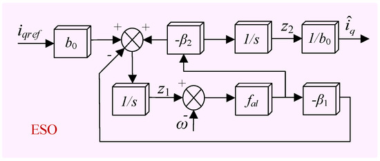
Figure 2. Structural diagram of ESO.

4. Simulation and Experimental Analysis

4.1. Analysis of Simulation

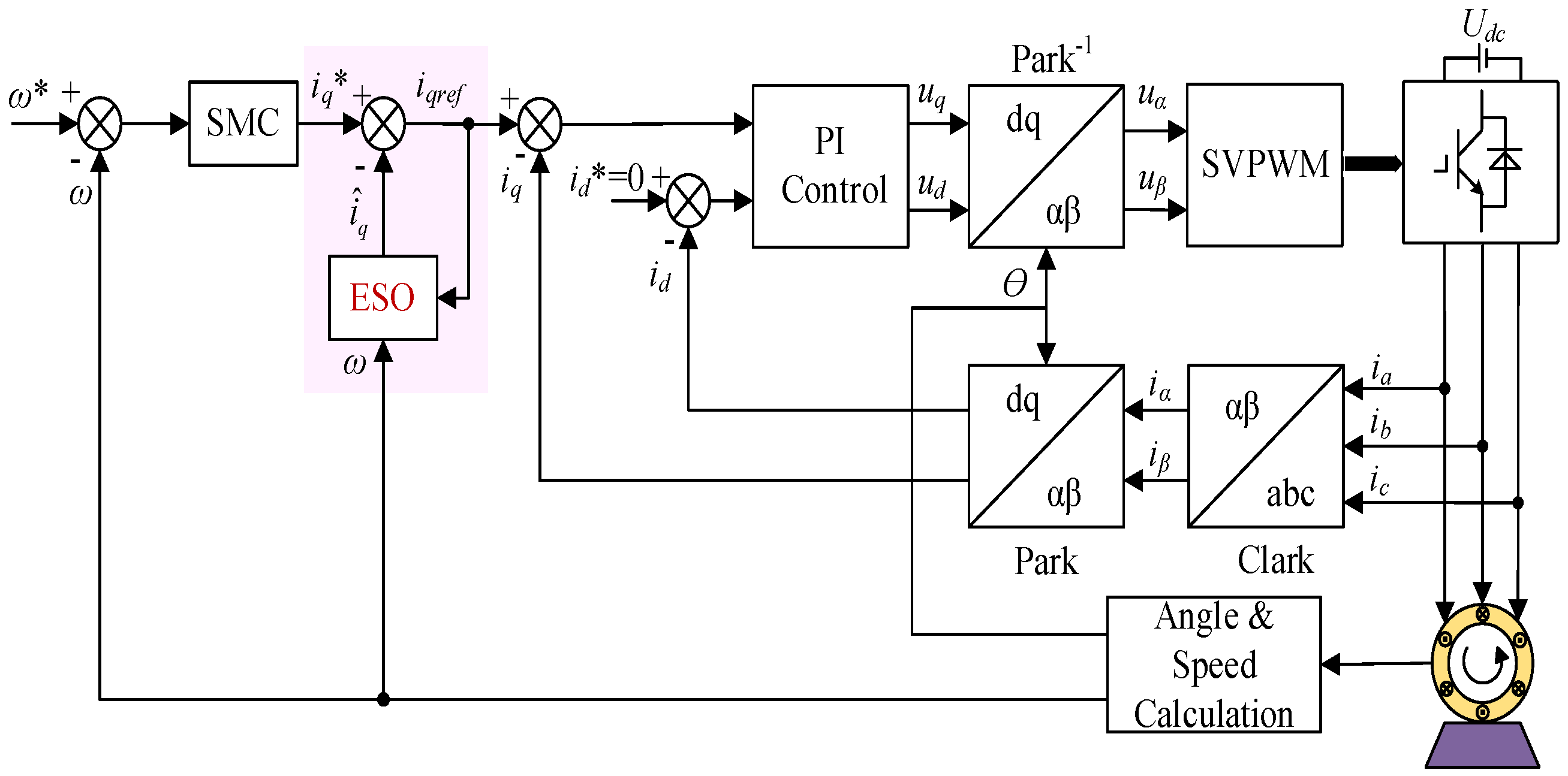
To validate the aforementioned control method, the vector control model of PMSM depicted in Figure 3 was initially constructed in Simulink 1.0. This model encompasses components such as the vector system, ESO, SMC, the motor under control, and others. In this model, the inner loop current is regulated by PID control. Simulation is carried out, and comparisons are made with conventional SMC and PID. The parameters of PMSM employed in the simulation are shown in Table 1. The selection of the sliding surface parameters and convergence speed parameters follows the values defined by the motor parameter design. Additionally, the parameters of ESO are mainly derived from the motor speed output state equation and ADRC. This overall configuration allows for a systematic assessment of the performance and effectiveness of the proposed control method in the simulated PMSM control scenario.

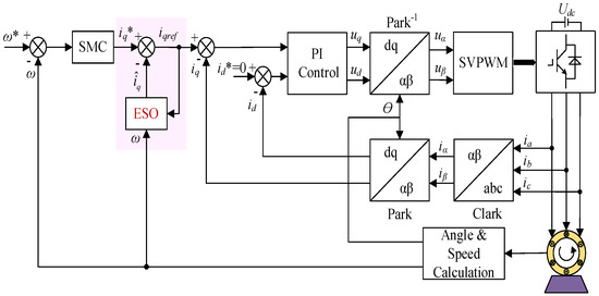
Figure 3. Overall block diagram of the control system.

Table 1. Parameters of the simulated motor.

Parameter	Value
Stator phase resistance (Rs)	2.875 Ω
Inductance (Ld)	8.5 × 10−3 H
Inductance (Lq)	8.5 × 10−3 H
Flux linkage (Ψf)	0.175 Wb
Inertia (J)	1.6 × 10−3 kg·m2
Pole pairs (p)	4
Viscous friction coefficient (B)	3 × 10−4 N·m·s/rad

In order to further analyze the effect of the five parameters in the ESO on the PMSM speed, the five parameters will be changed sequentially to observe the motor speed.

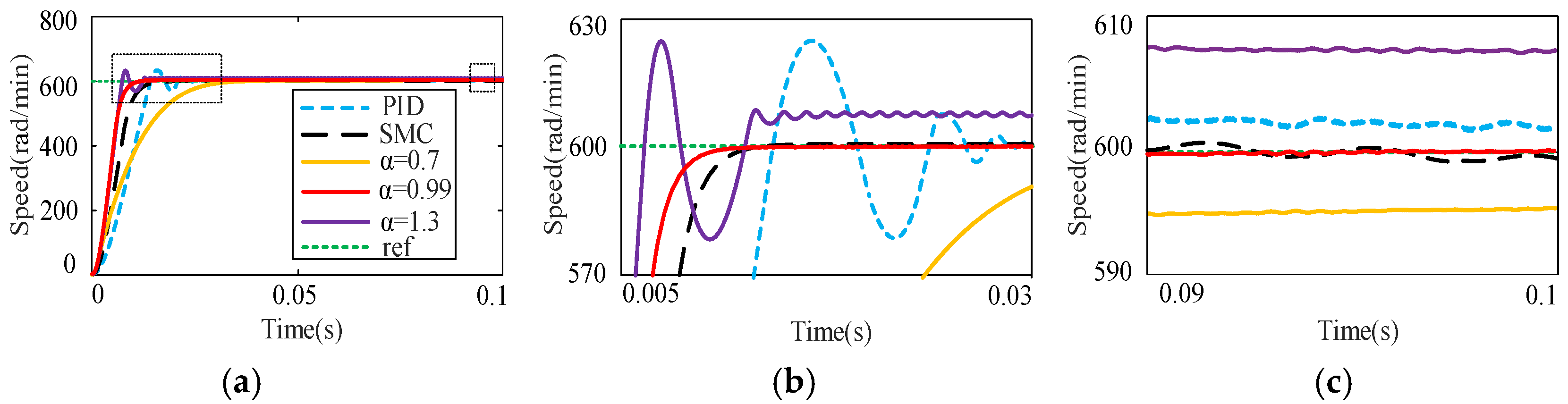
As shown in Figure 4, the value of α is generally taken as 0 < α < 1. The simulation shows that when α is larger than 1, the motor output is very poor and has deviated from the original state, and a smaller α causes the regulation time for the motor to reach the reference speed to grow and increase the steady state error [23].

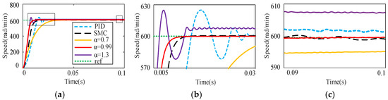
Figure 4. Simulation results of startup response under different α. (a) Speed response of startup. (b) Overshoot and adjustment time. (c) Steady-state error.

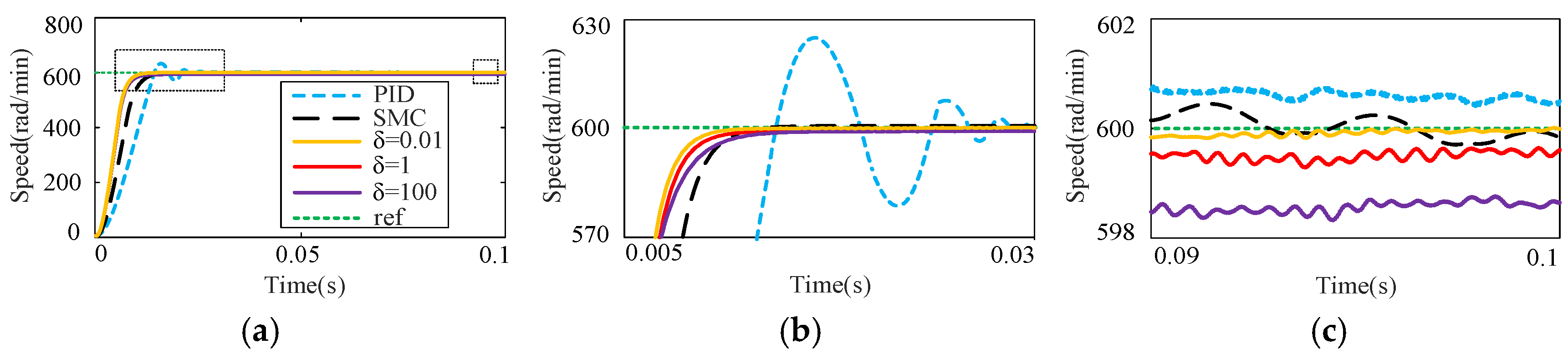
An appropriate filtering factor δ can effectively filter and also affect the rate at which the system reaches its true state, and because the filtering factor δ is too high, from f_al(e, α, δ) = e/δ^1−α, (e < δ), error e will gradually converge from a large range, as shown in Figure 5. When starting, with the increase in δ, the speed will enter the deceleration stage in advance. The steady-state error is also large, and the fluctuation range is large. Therefore, when δ is too large, it may affect the system’s instability, especially when dealing with high-frequency interference. It may introduce more noise, resulting in an increase in the error of motor output. Therefore, the filter factor cannot easily take too large a value.

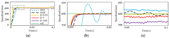
Figure 5. Simulation results of startup response under different δ. (a) Speed response of startup. (b) Overshoot and adjustment time. (c) Steady-state error.

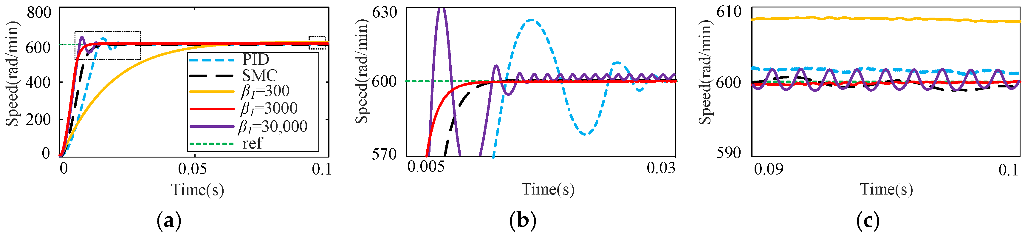
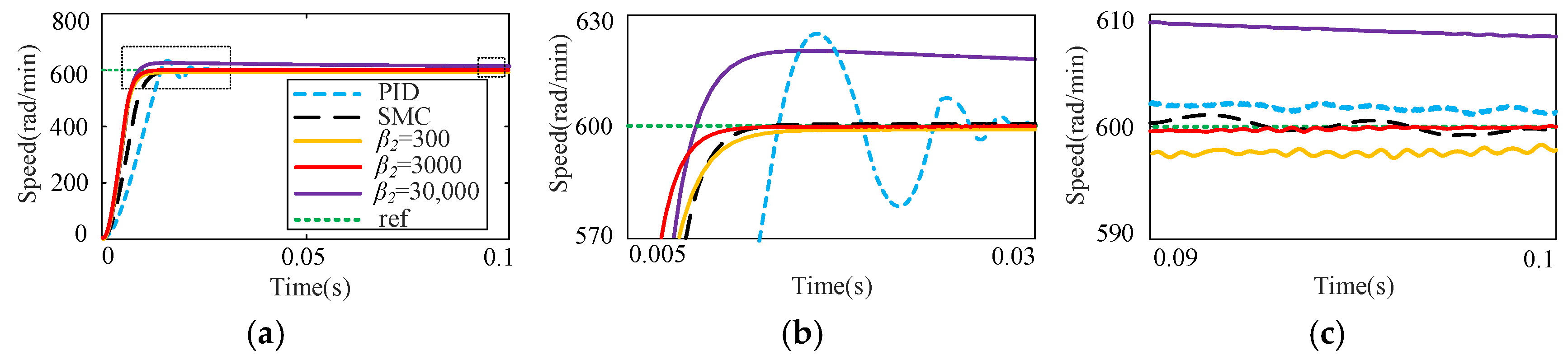
As shown in Figure 6 and Figure 7, as the values of parameters β₁ and β₂ increase, the response time of the motor decreases, but at the same time the amount of overshooting will occur and will oscillate to the point of instability, and if the values of β₁ and β₂ are too small, the error of the motor output will also increase. The parameters β₁ and β₂ are related to the sampling step size of the system [23].

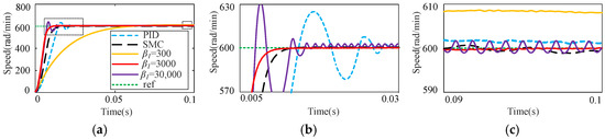
Figure 6. Simulation results of startup response under different β₁. (a) Speed response of startup. (b) Overshoot and adjustment time. (c) Steady-state error.

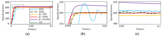
Figure 7. Simulation results of startup response under different β₂. (a) Speed response of startup. (b) Overshoot and adjustment time. (c) Steady-state error.

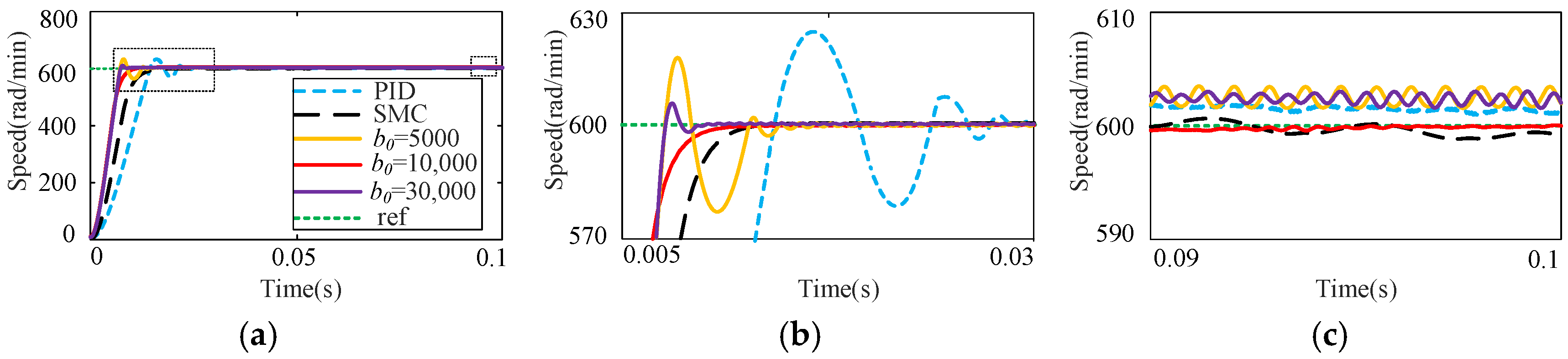
The size of b₀ is mainly determined by the system parameters, as shown in Figure 8, a larger or smaller b₀ will result in overshooting and oscillations.

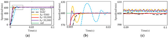
Figure 8. Simulation results of startup response under different b₀. (a) Speed response of startup. (b) Overshoot and adjustment time. (c) Steady-state error.

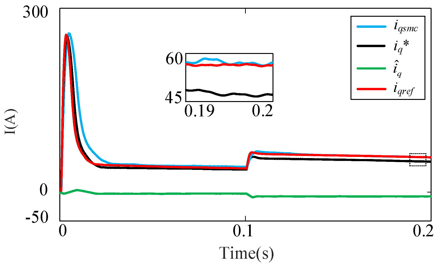
When selecting the appropriate parameters to observe the output current i_qref waveform after adding the disturbance observer as shown in Figure 9, with 0 s start, 0.1 s to give a certain load, it can be analyzed that the disturbance observer compensates for the sliding mode output current i_q^*. In the early stage of the response, compensating for the negative current, the actual output reference current i_qref increases, which makes the motor speed rise rapidly. In the late stage of the response, compensating for the positive current, decreasing the output. In the late response period, the positive current is compensated and the output reference current i_qref is reduced, so that the motor reaches a stable state quickly. Moreover, the output current jitter is reduced after compensation, which further reduces the steady state error when the motor is running stably. Compared to the conventional SMC current i_qsmc, the improved method has better current performance.

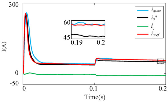
Figure 9. Real-time demanded current observer.

When determining the simulation control parameters as shown in Table 2, the motor is set to verify the control performance of the controller under different conditions. The motor speed was compared under PI, SMC, and SMC-ESO.

Table 2. Parameters of controller.

Control Structure	Control Parameters
Speed Control	SMC	c = 50 k = 25 d = −1 ε = 30 A = 12,500
	ESO	α = 0.99 δ = 0.01 b0 = 12,500 β1 = 3000 β2 = 3000
Current Control	PI	Kpq = 2 Kiq = 1 Kpd = 2 Kid = 1

The first experiment involves starting the motor to 600 rad/min under no-load conditions and observing response of the motor, as shown in Figure 10.

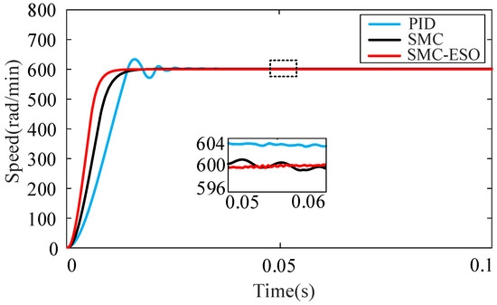
Figure 10. Simulation results of response of startup.

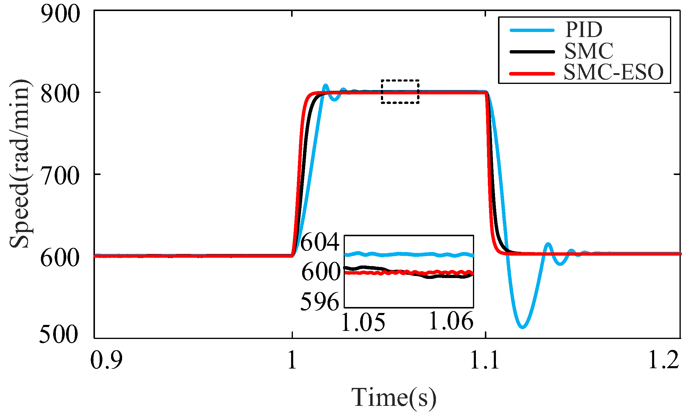
The second experiment was conducted under no-load conditions, with the range of speed changes from 600 rad/min to 800 rad/min and from 800 rad/min to 600 rad/min. The speed of the motor when the reference speed changes is shown in Figure 11.

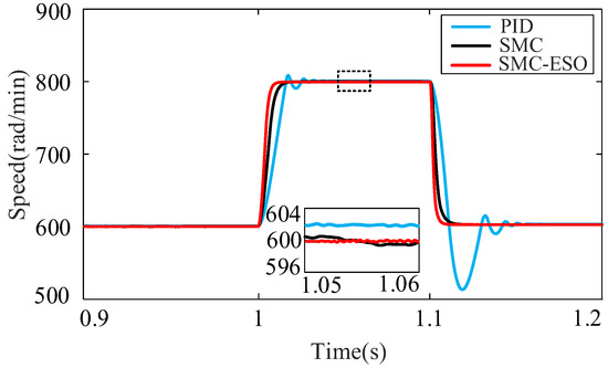
Figure 11. Simulation results of response of speed change.

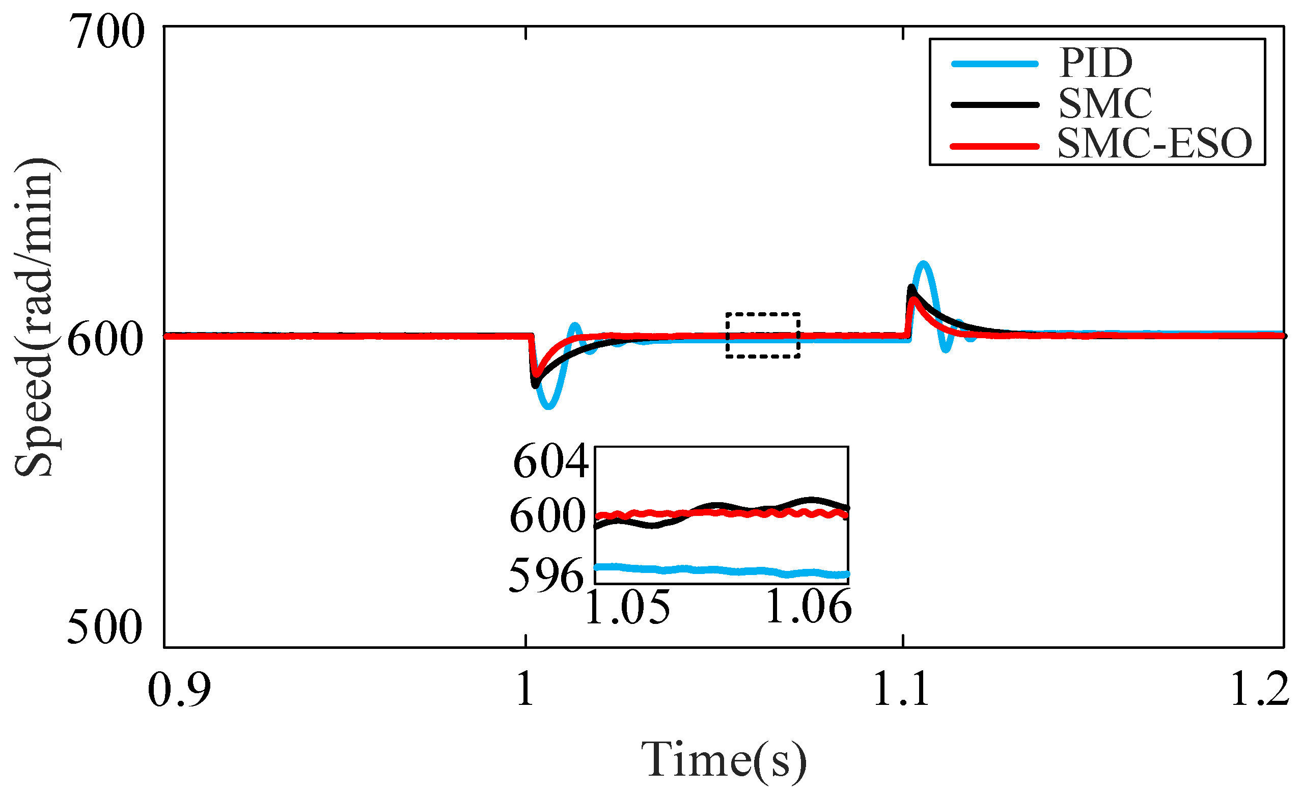
The third experiment was conducted under no-load conditions of 600 rad/min, with the motor load rises from no-load to 5 NM and fall from 5 NM to no-load. The motor speed and current were observed under load changes, as shown in Figure 12. The motor outputs a phase current, as shown in Figure 13.

Figure 12. Simulation results of response of load change.

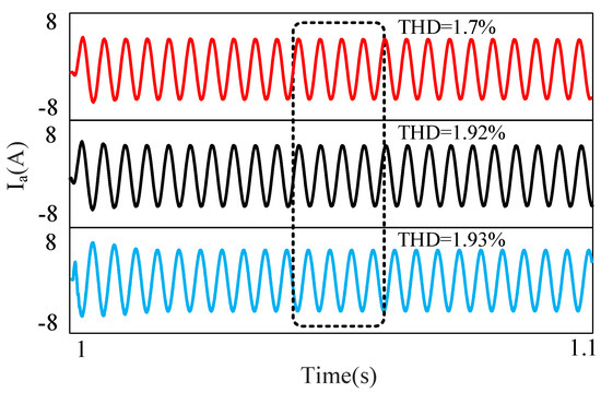
Figure 13. Simulation results of a-phase current with load.

Figure 10, Figure 11 and Figure 12 show that the new control method has less chattering and faster response, and more robustness under different operating conditions. Figure 13 shows that there is less stator current impingement, faster response, and less harmonic content in steady state when load torque is added.

4.2. Results of Experimental

In order to validate the methodology of this paper, the adopted open-source motor rapid control simulation platform based on Rapid Control Prototyping (RCP) is shown in Figure 14, in which the control model is built in MATLAB R2023a, and the necessary operating information of the system is given in the upper computer via the StarSim. The parameters of PMSM used are shown in Table 3.

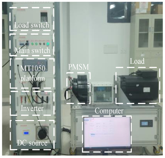
Figure 14. Experimental platform.

Table 3. Parameters of PMSM.

Parameters	Value	Parameters	Value
Rated Power	6 KW	Rated Speed	800 rpm
Rated Voltage	144 V	Rated Torque	35 Nm
Rated Current	50 A	Number of pole pairs	24

The experiments are conducted in accordance with the simulation methodology.

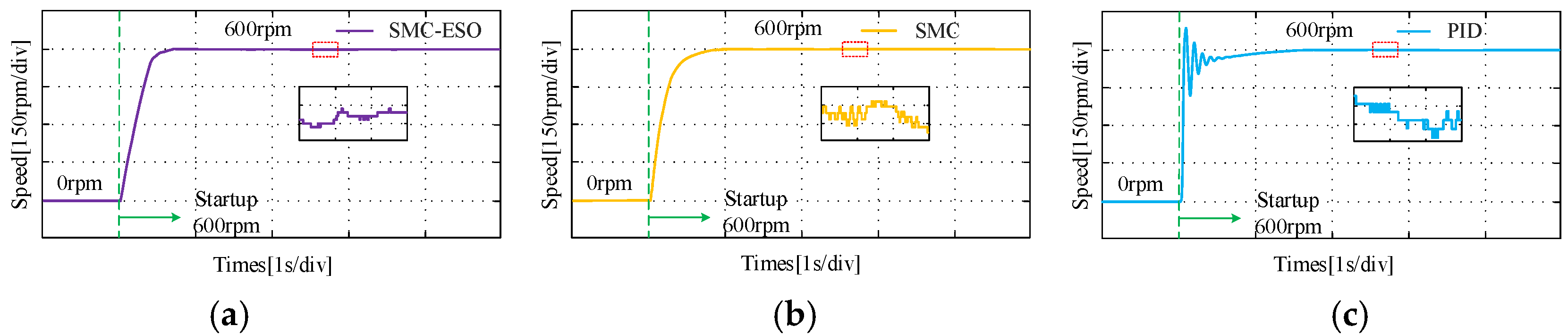
In the first experiments, under no-load conditions, the given speed is set to 600 rad/min, as illustrated in Figure 15.

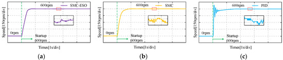
Figure 15. Experimental results of response of startup under different control strategies. (a) SMC-ESO. (b) SMC. (c) PID.

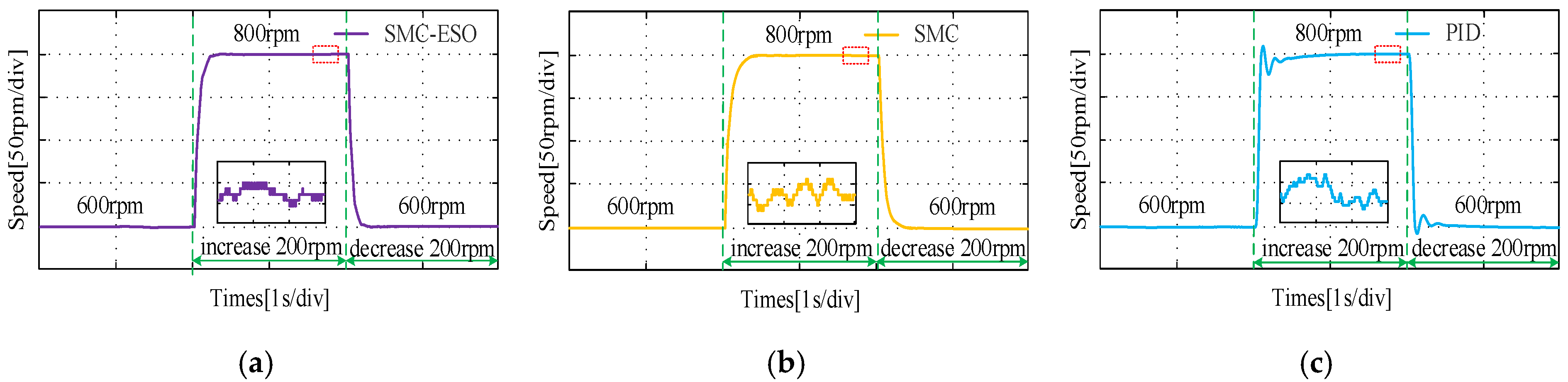
In the second experiment, within the no-load scenario, the speed varies between 600 rad/min to 800 rad/min and then from 800 rad/min to 600 rad/min, as depicted in Figure 16.

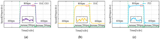
Figure 16. Experimental results of response of speed change under different control strategies. (a) SMC-ESO. (b) SMC. (c) PID.

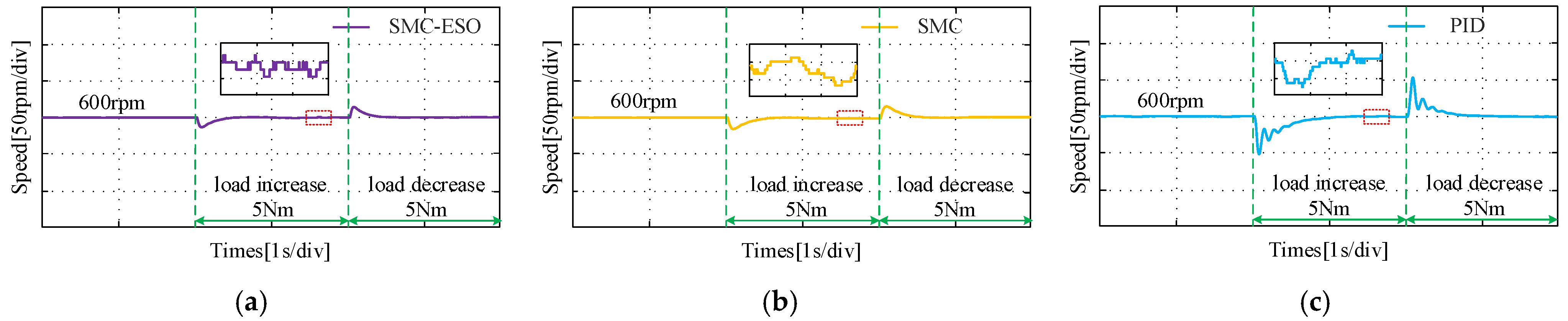
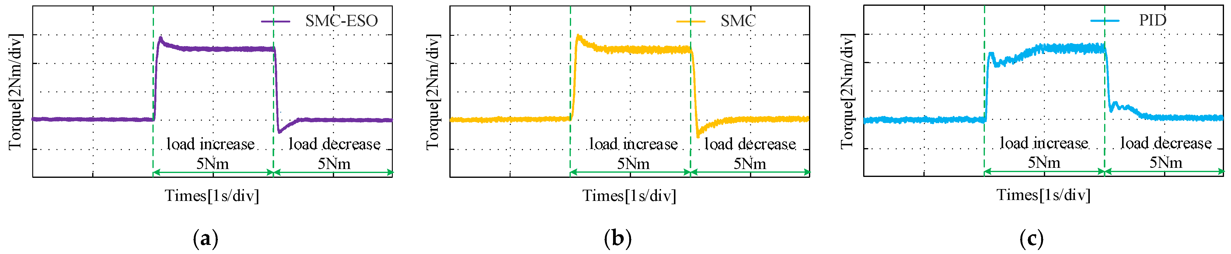
In the third experiment, commencing from a base speed of 600 rad/min, the motor load increases from no-load to 5 N·m and subsequently decreases from 5 N·m back to no-load, as shown in Figure 17.

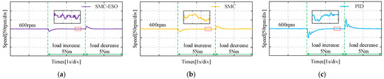
Figure 17. Experimental results of response to load change under different control strategies. (a) SMC-ESO. (b) SMC. (c) PID.

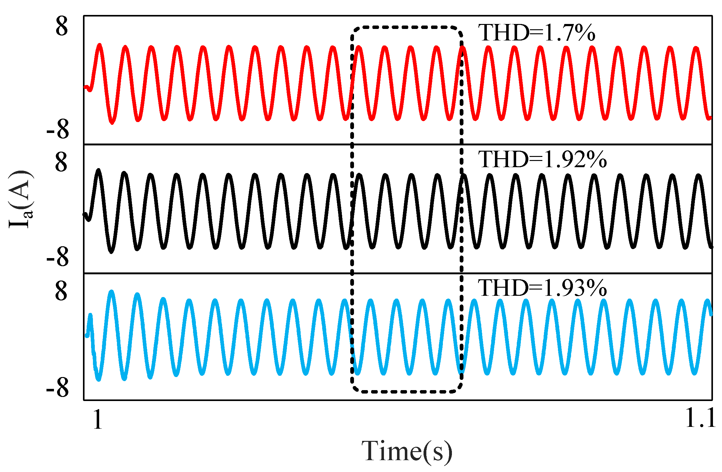
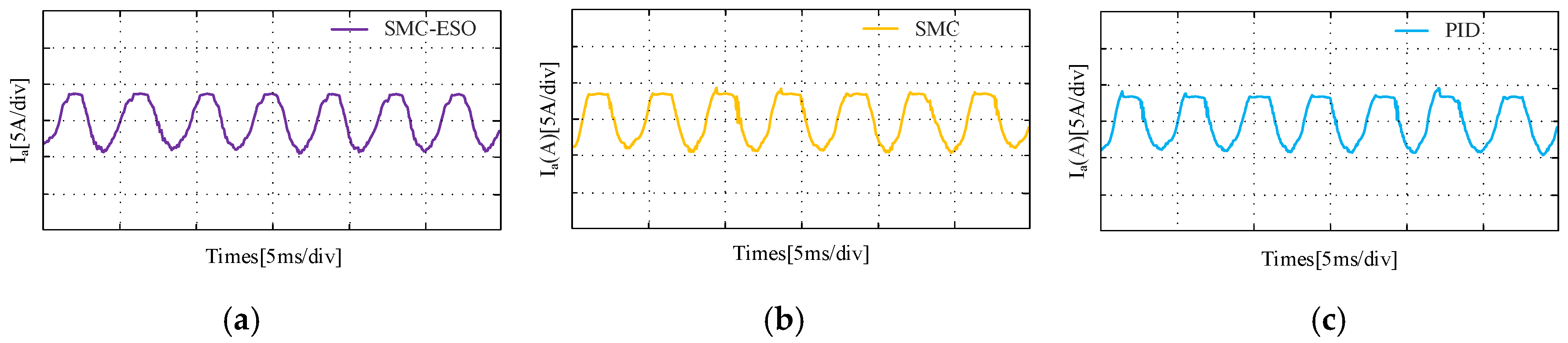
Figure 18 presents the output torque during the load change process. Figure 19 shows the a-phase current under loaded operation. The experimental results demonstrate that the output torque regulated by the SMC-ESO approach is more precise, and the harmonic content in the output current is lower. This indicates the superiority of the SMC-ESO in enhancing the control performance.

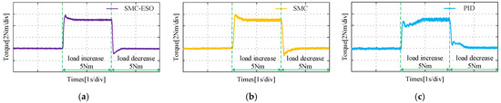
Figure 18. Experimental results of torque output of load change under different control strategies. (a) SMC-ESO. (b) SMC. (c) PID.

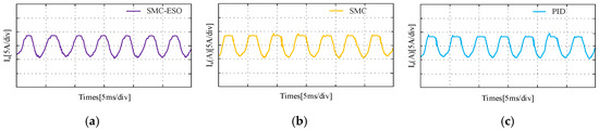
Figure 19. Experimental results of a-phase current with load under different control strategies. (a) SMC-ESO. (b) SMC. (c) PID.

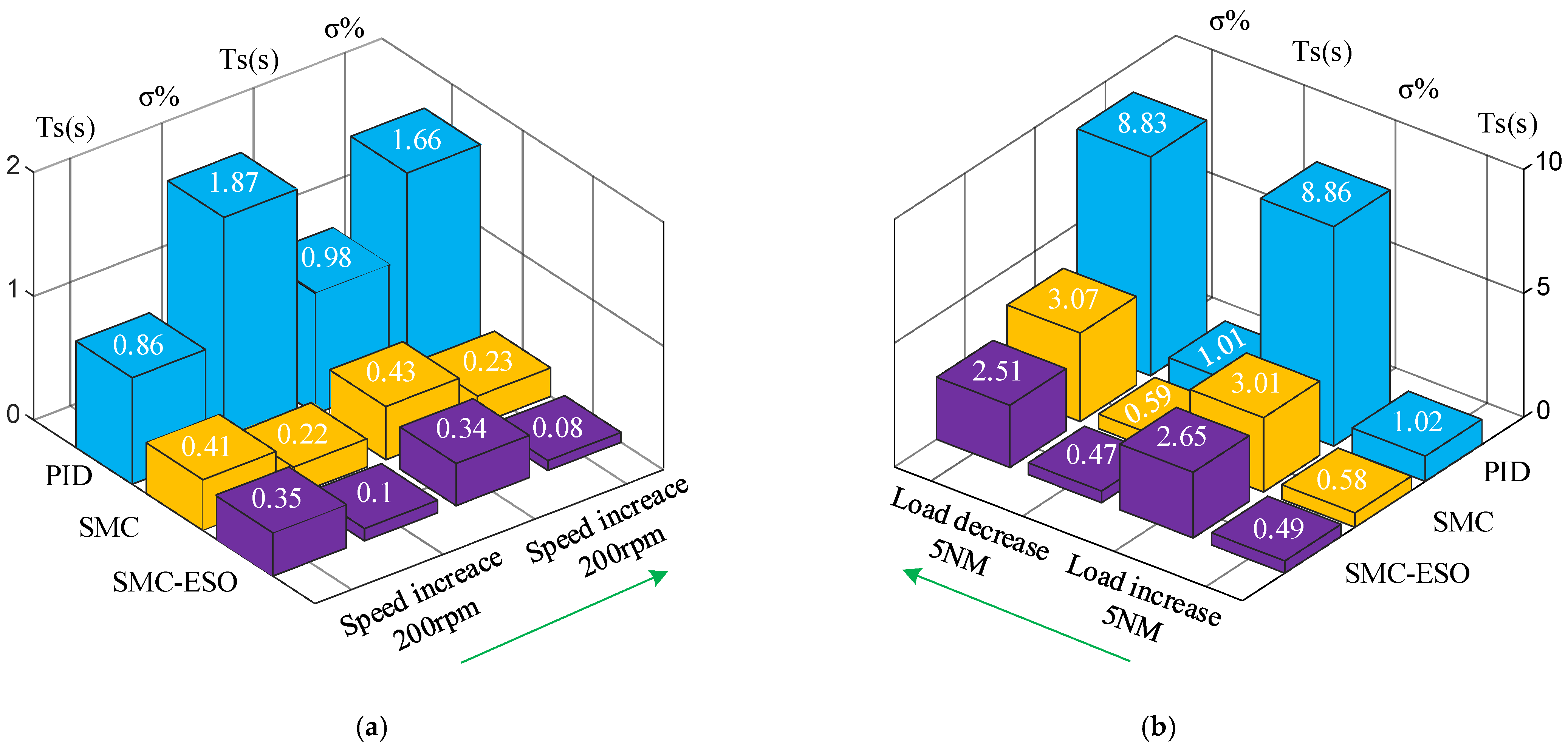
The experimental data of three control strategies during speed and load changes are shown in Figure 20. Compared with conventional SMC, SMC-ESO has reduced response time by 30% during speed changes, reduced jitter by 59%, reduced speed fluctuations by 15% during load changes, and reduced response time by 18%, making it more robust.

Figure 20. Experimental data of the response under different control strategies during disturbance. (a) Speed change. (b) Load change.

5. Conclusions

In this paper, a new sliding mode control for PMSM has been studied, and it has been compared to conventional sliding mode control. The conclusions are as follows:

(1)

Due to the motion trajectory of sliding mode control moving back and forth on the sliding surface and eventually converging to a steady state, it is prone to jitter and vibration.

(2)

Real time observation and compensation of q-axis current by current observers can achieve stable control under interference and small jitter. Simulation and experimental results show that SMC-ESO improves dynamic and steady-state performance of PMSM.

(3)

Due to the current fluctuation observer, the motor can be used in more complex and high-precision operating environments, and this control method can be easily applied to practical industries without additional implementation costs.

References

- Dong, H.; Yang, X.; Gao, H.; Yu, X. Practical Terminal Sliding-Mode Control and Its Applications in Servo Systems. IEEE Trans. Ind. Electron. 2023, 70, 752–761. [Google Scholar] [CrossRef]
- Wang, H.; Li, S.; Yang, J.; Zhou, X. Continuous Sliding Mode Control for Permanent Magnet Synchronous Motor Speed Regulation Systems Under Time-Varying Disturbances. J. Power Electron. 2016, 16, 1324–1335. [Google Scholar] [CrossRef]
- Apte, A.; Joshi, V.A.; Mehta, H.; Walambe, R. Disturbance-Observer-Based Sensorless Control of PMSM Using Integral State Feedback Controller. IEEE Trans. Power Electron. 2020, 35, 6082–6090. [Google Scholar] [CrossRef]
- Zhang, Y.; Yin, Z.; Zhang, Y.; Liu, J.; Tong, X. A Novel Sliding Mode Observer with Optimized Constant Rate Reaching Law for Sensorless Control of Induction Motor. IEEE Trans. Ind. Electron. 2020, 67, 5867–5878. [Google Scholar] [CrossRef]
- Tian, M.; Wang, B.; Yu, Y.; Dong, Q.; Xu, D. Discrete-Time Repetitive Control-Based ADRC for Current Loop Disturbances Suppression of PMSM Drives. IEEE Trans. Ind. Inform. 2022, 18, 3138–3149. [Google Scholar] [CrossRef]
- Abu-Ali, M.; Berkel, F.; Manderla, M.; Reimann, S.; Kennel, R.; Abdelrahem, M. Deep Learning-Based Long-Horizon MPC: Robust, High Performing, and Computationally Efficient Control for PMSM Drives. IEEE Trans. Power Electron. 2022, 37, 12486–12501. [Google Scholar] [CrossRef]
- Pang, S.; Zhang, Y.; Huangfu, Y.; Li, X.; Tan, B.; Li, P.; Tian, C.; Quan, S. A Virtual MPC-Based Artificial Neural Network Controller for PMSM Drives in Aircraft Electric Propulsion System. IEEE Trans. Ind. Appl. 2024, 60, 3603–3612. [Google Scholar] [CrossRef]
- Li, H.; Wang, S.; Xie, Y.; Zheng, S.; Shi, P. Virtual Reference-Based Fuzzy Noncascade Speed Control for PMSM Systems with Unmatched Disturbances and Current Constraints. IEEE Trans. Fuzzy Syst. 2023, 31, 4249–4261. [Google Scholar] [CrossRef]
- Chaoui, H.; Khayamy, M.; Aljarboua, A.A. Adaptive Interval Type-2 Fuzzy Logic Control for PMSM Drives with a Modified Reference Frame. IEEE Trans. Ind. Electron. 2017, 64, 3786–3797. [Google Scholar] [CrossRef]
- El-Sousy, F.F.M.; Amin, M.M.; Al-Durra, A. Adaptive Optimal Tracking Control Via Actor-Critic-Identifier Based Adaptive Dynamic Programming for Permanent-Magnet Synchronous Motor Drive System. IEEE Trans. Ind. Appl. 2021, 57, 6577–6591. [Google Scholar] [CrossRef]
- Zuo, Y.; Lai, C.; Galkina, A.; Grossbichler, M.; Iyer, L.V. Adaptive Current Observer Design for Single Current Sensor Control in PMSM Drives. IEEE Trans. Transport. Electrif. 2024, 10, 6928–6939. [Google Scholar] [CrossRef]
- Tang, P.; Zhao, Z.; Li, H. Short-Term Prediction Method of Transient Temperature Field Variation for PMSM in Electric Drive Gearbox Using Spatial-Temporal Relational Graph Convolutional Thermal Neural Network. IEEE Trans. Ind. Electron. 2024, 71, 7839–7852. [Google Scholar] [CrossRef]
- Nguyen, T.H.; Nguyen, T.T.; Nguyen, V.Q.; Le, K.M.; Tran, H.N.; Jeon, J.W. An Adaptive Sliding-Mode Controller with a Modified Reduced-Order Proportional Integral Observer for Speed Regulation of a Permanent Magnet Synchronous Motor. IEEE Trans. Ind. Electron. 2022, 69, 7181–7191. [Google Scholar] [CrossRef]
- Xu, B.; Zhang, L.; Ji, W. Improved Non-Singular Fast Terminal Sliding Mode Control with Disturbance Observer for PMSM Drives. IEEE Trans. Transport. Electrif. 2021, 7, 2753–2762. [Google Scholar] [CrossRef]
- Li, S.; Zhou, M.; Yu, X. Design and Implementation of Terminal Sliding Mode Control Method for PMSM Speed Regulation System. IEEE Trans. Ind. Inform. 2013, 9, 1879–1891. [Google Scholar] [CrossRef]
- Hu, Q.; Liu, L.; Yang, H. A sliding mode speed controller based on novel reaching law of permanent magnet synchronous motor system. In Proceedings of the 2017 Chinese Automation Congress (CAC), Jinan, China, 20–22 October 2017; pp. 954–958. [Google Scholar]
- Junejo, A.K.; Xu, W.; Mu, C.; Ismail, M.M.; Liu, Y. Adaptive Speed Control of PMSM Drive System Based a New Sliding-Mode Reaching Law. IEEE Trans. Power Electron. 2020, 35, 12110–12121. [Google Scholar] [CrossRef]
- Zhang, Z.; Yang, X.; Wang, W.; Chen, K.; Cheung, N.C.; Pan, J. Enhanced Sliding Mode Control for PMSM Speed Drive Systems Using a Novel Adaptive Sliding Mode Reaching Law Based on Exponential Function. IEEE Trans. Ind. Electron. 2024, 71, 11978–11988. [Google Scholar] [CrossRef]
- Guo, X.; Huang, S.; Lu, K.; Peng, Y.; Wang, H.; Yang, J. A Fast Sliding Mode Speed Controller for PMSM Based on New Compound Reaching Law With Improved Sliding Mode Observer. IEEE Trans. Transport. Electrif. 2023, 9, 2955–2968. [Google Scholar] [CrossRef]
- Wang, Y.; Feng, Y.; Zhang, X.; Liang, J.; Cheng, X. New Reaching Law Control for Permanent Magnet Synchronous Motor with Extended Disturbance Observer. IEEE Access 2019, 7, 186296–186307. [Google Scholar] [CrossRef]
- Xu, W.; Qu, S.; Zhang, C. Fast Terminal Sliding Mode Current Control with Adaptive Extended State Disturbance Observer for PMSM System. IEEE J. Emerg. Sel. Top. Power Electron. 2023, 11, 418–431. [Google Scholar] [CrossRef]
- Long, K.; Zhang, X.; Xi, Z.; Li, N. Neural network sliding mode control based on improved fruit-fly optimization algorithm for permanent magnet synchronous motor systems. In Proceedings of the 2022 5th International Conference on Advanced Electronic Materials, Computers and Software Engineering (AEMCSE), Wuhan, China, 22–24 April 2022; pp. 488–491. [Google Scholar]
- Han, J. From PID to Active Disturbance Rejection Control. IEEE Trans. Ind. Electron. 2009, 56, 900–906. [Google Scholar] [CrossRef]
Disclaimer/Publisher’s Note: The statements, opinions and data contained in all publications are solely those of the individual author(s) and contributor(s) and not of MDPI and/or the editor(s). MDPI and/or the editor(s) disclaim responsibility for any injury to people or property resulting from any ideas, methods, instructions or products referred to in the content. |
© 2025 by the authors. Licensee MDPI, Basel, Switzerland. This article is an open access article distributed under the terms and conditions of the Creative Commons Attribution (CC BY) license (https://creativecommons.org/licenses/by/4.0/).