Fuzzy Flocking Control for Multi-Agents Trapped in Dynamic Equilibrium Under Multiple Obstacles

Abstract

The Olfati-Saber flocking (OSF) algorithm is widely used in multi-agent flocking control due to its simplicity and effectiveness. However, this algorithm is prone to trapping multi-agents in dynamic equilibrium under multiple obstacles, and dynamic equilibrium is a key technical issue that needs to be addressed in multi-agent flocking control. To overcome this problem, we propose a dynamic equilibrium judgment rule and design a fuzzy flocking control (FFC) algorithm. In this algorithm, the expected velocity is divided into fuzzy expected velocity and projected expected velocity. The fuzzy expected velocity is designed to make the agent escape from the dynamic equilibrium, and the projected expected velocity is designed to tow the agent, bypassing the obstacles. Meanwhile, the sensing radius of the agent is divided into four subregions, and a nonnegative subsection function is designed to adjust the attractive/repulsive potentials in these subregions. In addition, the virtual leader is designed to guide the agent in achieving group goal following. Finally, the experimental results show that multi-agents can escape from dynamic equilibrium and bypass obstacles at a faster velocity, and the minimum distance between them is consistently greater than the minimum safe distance under complex environments in the proposed algorithm.

1. Introduction

Flocking is a cluster composed of a large number of agents, enabling the system to achieve overall coordination through the behaviors of individual agents [1,2,3]. To date, there have been a lot of studies on the control of coordination behaviors generated by agents, including flocking control [4,5], consensus control [6,7], and formation control [8,9], to name a few.

Flocking control is the basis for investigating consensus control and formation control. Olfati-Saber [10] proposed a flocking control algorithm. In this algorithm, collisions between agents and between the agent and obstacles are avoided by virtual attractive/repulsive potential, velocity matching between agents is achieved by the velocity consensus term, and goal following is realized by virtual leaders. Meanwhile, flocking control has been extensively investigated by numerous researchers [11,12,13]. From the perspective of virtual leaders, current research on flocking control can be divided into each agent with virtual leader information [14,15,16], some agents with virtual leader information [17,18], and multi-agents with multiple virtual leaders’ information [19]. Overall, the aforementioned studies have contributed to the advancement of multi-agent flocking control based on virtual leaders. However, it is noted in [20,21,22] that some agents fail to follow the virtual leader in multiple obstacle environments. The reason is that the virtual forces of these agents have reached equilibrium with near-zero acceleration and velocity, which is referred to as dynamic equilibrium. Therefore, the virtual force problem of multi-agents in multiple obstacle environments is critical in flocking control research [23].

At present, the methods to solve the virtual force problem mainly include the geometric filling [24,25] and intelligent decision-making methods [26,27,28]. In the geometric filling method, it is generally assumed that the agent has the ability to perceive global obstacle information. Furthermore, to change the virtual force of the agent under multiple obstacles such that it can follow the goal, the non-convex obstacles are transformed into convex ones via geometric filling rules, followed by the generation of virtual agents on their surface. In the intelligent decision-making method, the agent is first trained in multiple obstacle environments to form obstacle avoidance movement rules. Then, the obstacle information perceived by the agent is utilized to match with the training model, producing the virtual force for obstacle avoidance and goal following. On the whole, the geometric filling and intelligent decision-making methods enable multi-agents to escape from the dynamic equilibrium. The geometric filling method requires the obtaining of global obstacle information, which limits its practical application. The intelligent decision-making method involves a complex training structure, and the real-time performance requires further improvement. In addition, these methods suffer from the multi-attribute decision-making problem.

Fuzzy control is an effective method for solving the multi-attribute decision-making problem [29,30]. In [31], the attractive/repulsive function is designed by the fuzzy control method, thus proposing a multi-agent flocking control algorithm with obstacle avoidance. The computational complexity of this algorithm is low. However, it is possible for the agent to be trapped in dynamic equilibrium when perceiving multiple obstacles. Motivated by the above studies, this paper attempts to calculate the fuzzy expected velocity by the established membership functions and fuzzy rules, which enable the agent to escape from the dynamic equilibrium. The contributions of this paper are summarized as follows:

(1)

A dynamic equilibrium judgment rule is proposed to determine whether the agent is trapped in dynamic equilibrium. If the agent is trapped in dynamic equilibrium, the fuzzy expected velocity is calculated by the established membership functions and fuzzy rules. In contrast, if the agent is not trapped, the projected expected velocity is obtained by the obstacle projection method.

(2)

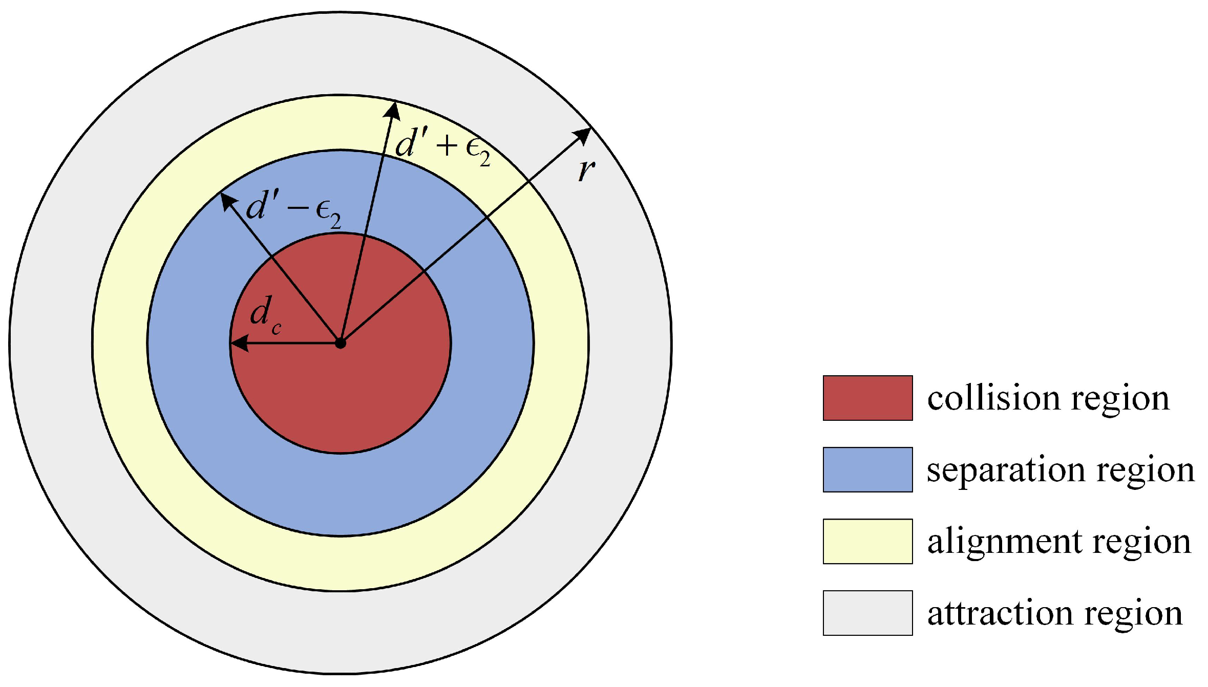
The sensing radius region of the agent is divided into four subregions and a nonnegative subsection function is designed to adjust the attractive/repulsive potentials in these subregions.

(3)

A fuzzy flocking control (FFC) algorithm is developed for multi-agents trapped in dynamic equilibrium under multiple obstacles. In the algorithm, the interaction term between agents is reconstructed using the fuzzy expected velocity, projected expected velocity, and nonnegative subsection function.

The remainder of this paper is organized as follows. Some preliminary knowledge is introduced in Section 2. In Section 3, the FFC algorithm is proposed. In Section 4, the properties analysis of the FFC algorithm is presented. Numerical experiments and the discussion are reported in Section 5. The conclusions are given in Section 6.

2. Preliminaries

2.1. Agent-Based Representation

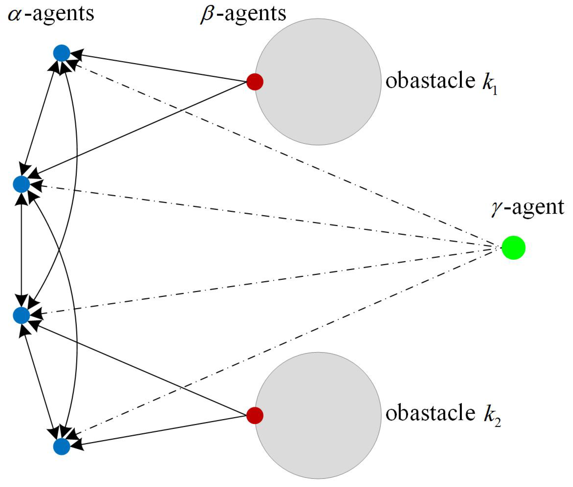
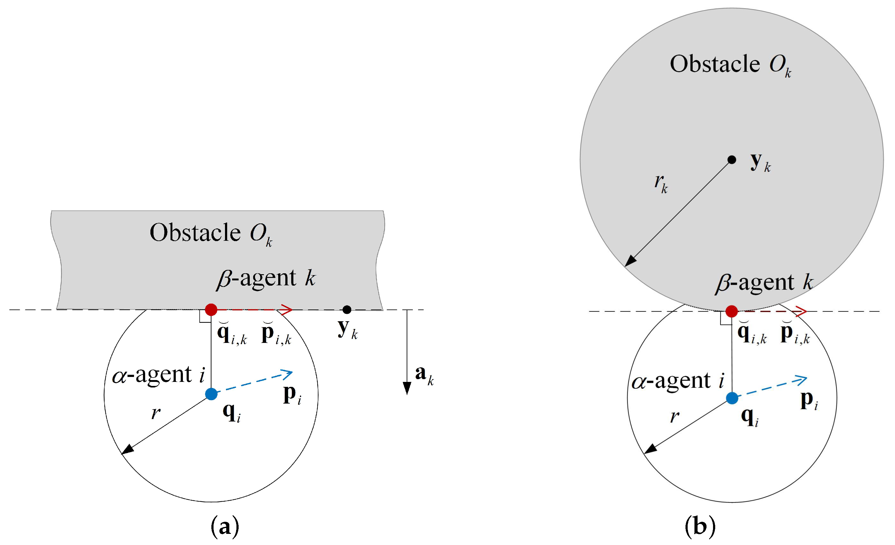
Consider a group of N $\alpha$-agents moving in the n-dimensional Euclidean space, $n=2,3$. Denote ${\mathbf{q}}_i,{\mathbf{p}}_i,{\mathbf{u}}_i\in {\mathbb{R}}^{n\times 1}$ as the position, velocity, and control input (or acceleration) acting on $\alpha$-agent i, $i=1,2,\dots ,N$ at the current time. Then, the second-order dynamic model of $\alpha$-agent i can be formulated as:

$$\left\{\begin{array}{c}{\dot{\mathbf{q}}}_i=\delta {\mathbf{p}}_i+(1-\delta )p_{i,m}{\displaystyle \frac{{\mathbf{p}}_i}{\parallel {\mathbf{p}}_i\parallel }}\hfill \\ {\dot{\mathbf{p}}}_i={\mathbf{u}}_i\hfill \end{array}\right.$$

(1)

where $p_{i,m}$ represents the upper velocity limit of $\alpha$-agent i, $\delta =1$ if $\parallel {\mathbf{p}}_i\parallel \le p_{i,m}$, otherwise $\delta =0$, ${\dot{\mathbf{q}}}_i$ denotes the first order derivative of the vector ${\mathbf{q}}_i$, and $\parallel {\mathbf{q}}_i\parallel$ represents the Euclidean norm of the vector ${\mathbf{q}}_i$. Furthermore, a virtual $\gamma$-agent (e.g., multi-drone precision firefighting and multi-robot rescue) is introduced to achieve group goal following. Denote ${\mathbf{q}}^{\gamma },{\mathbf{p}}^{\gamma },{\mathbf{u}}^{\gamma }\in {\mathbb{R}}^{n\times 1}$ as the position, velocity, and control input acting on the $\gamma$-agent at the current time. Then, the second-order dynamic model of the $\gamma$-agent can be described as:

$$\left\{\begin{array}{c}{\dot{\mathbf{q}}}^{\gamma }={\mathbf{p}}^{\gamma }\hfill \\ {\dot{\mathbf{p}}}^{\gamma }={\mathbf{u}}^{\gamma }\hfill \end{array}\right.$$

(2)

2.2. Proximity Net of $\alpha$-Agents and $\beta$-Agents

The flocking composed of N $\alpha$-agents can be described by an undirected graph ${\mathcal{G}}^{\alpha }\left(\mathbf{q}\right)=({\mathcal{V}}^{\alpha },{\mathcal{E}}^{\alpha }\left(\mathbf{q}\right))$, where ${\mathcal{V}}^{\alpha }=\{1,2,\dots ,N\}$ is the set of $\alpha$-agent nodes, ${\mathcal{E}}^{\alpha }\left(\mathbf{q}\right)=\{(i,j)\mid i,j\in {\mathcal{V}}^{\alpha },j\ne i\}$ is the set of edges, and $\mathbf{q}$ is the configuration of all $\alpha$-agents. To avoid collisions between $\alpha$-agents and obstacles, a number of virtual $\beta$-agents are generated at the boundary points of obstacles. All $\beta$-agents can be described by a directed bipartite graph ${\mathcal{G}}^{\beta }\left(\mathbf{q}\right)=({\mathcal{V}}^{\beta },{\mathcal{E}}^{\beta }\left(\mathbf{q}\right))$, where ${\mathcal{V}}^{\beta }=\{v_1,v_2,\dots ,v_l\}$ is the set of $\beta$-agent nodes and ${\mathcal{E}}^{\alpha }\left(\mathbf{q}\right)=\{(i,k)\mid i\in {\mathcal{V}}^{\alpha },k\in {\mathcal{V}}^{\beta }\}$ is the set of edges. Then, the proximity net of $\alpha$-agents and $\beta$-agents can be described by

$$\mathcal{G}\left(\mathbf{q}\right)={\mathcal{G}}^{\alpha }\left(\mathbf{q}\right)+{\mathcal{G}}^{\beta }\left(\mathbf{q}\right)$$

(3)

Let r be the sensing radius, ${\mathcal{N}}_i^{\alpha }$ be the set of neighboring $\alpha$-agents of $\alpha$-agent i, ${\mathcal{N}}_i^{\beta }$ be the set of neighboring $\beta$-agents of $\alpha$-agent i, and ${\breve{\mathbf{q}}}_{i,k}$ be the position of $\beta$-agent k, then

$$\begin{array}{cc}\hfill {\mathcal{N}}_i^{\alpha }& =\{j\in {\mathcal{V}}^{\alpha }\mid \parallel {\mathbf{q}}_j-{\mathbf{q}}_i\parallel <r,i\in {\mathcal{V}}^{\alpha },j\ne i\}\hfill \end{array}$$

(4)

$$\begin{array}{cc}\hfill {\mathcal{N}}_i^{\beta }& =\{k\in {\mathcal{V}}^{\beta }\mid \parallel {\breve{\mathbf{q}}}_{i,k}-{\mathbf{q}}_i\parallel <r,i\in {\mathcal{V}}^{\alpha }\}\hfill \end{array}$$

(5)

2.3. Collective Potential Functions

The lattice-type structure can be used to capture the geometry between $\alpha$-agents and between the $\alpha$-agent and $\beta$-agent. In this structure, the distances between the $\alpha$-agent and its neighboring $\alpha$-agents are equal, as are the distances to its neighboring $\beta$-agents. Thus, the positions of $\alpha$-agents and $\beta$-agents are represented by the following constraints:

$$\begin{array}{cc}\hfill & \parallel {\mathbf{q}}_j-{\mathbf{q}}_i{\parallel }_{\sigma }=d_{\sigma }j\in {\mathcal{N}}_i^{\alpha }\hfill \end{array}$$

(6)

$$\begin{array}{cc}\hfill & \parallel {\breve{\mathbf{q}}}_{i,k}-{\mathbf{q}}_i{\parallel }_{\sigma }=d_{\sigma }^{\prime }k\in {\mathcal{N}}_i^{\beta }\hfill \end{array}$$

(7)

where ${\parallel ·\parallel }_{\sigma }={\displaystyle \frac{1}{{ϵ}_1}}[\sqrt{1+{ϵ}_1{\parallel ·\parallel }^2}-1]$, ${ϵ}_1>0$, $\parallel {\mathbf{q}}_j-{\mathbf{q}}_i\parallel =d$, $\parallel {\breve{\mathbf{q}}}_{i,k}-{\mathbf{q}}_i\parallel =d^{\prime }$, $d_{\sigma }={\parallel d\parallel }_{\sigma }$, $d_{\sigma }^{\prime }={\parallel d^{\prime }\parallel }_{\sigma }$, $d\le r$, and $d^{\prime }\le r$. To obtain the solutions of these constraints, it is necessary to construct two smooth collective potential functions ${\Phi }^{\alpha }\left(\mathbf{q}\right)$ and ${\Phi }^{\beta }\left(\mathbf{q}\right)$ such that their local minima correspond to the solutions of the constraints (6) and (7), respectively. The detailed construction procedure is described below:

First, the bump function ${\rho }_h\left(z\right)$ is introduced as

$$\begin{array}{c}\hfill {\rho }_h\left(z\right)=\left\{\begin{array}{cc}1,\hfill & z\in [0,h)\hfill \\ {\displaystyle \frac{1}{2}}\left[1+cos\left(\pi {\displaystyle \frac{(z-h)}{(1-h)}}\right)\right],\hfill & z\in [h,1]\hfill \\ 0,\hfill & \mathrm{otherwise}\hfill \end{array}\right.\end{array}$$

(8)

where $h\in (0, 1)$. Second, let ${\psi }^{\alpha }\left(z\right)$ be the pairwise attractive/repulsive potential between $\alpha$-agents and ${\psi }^{\beta }\left(z\right)$ be the pairwise attractive/repulsive potential between the $\alpha$-agent and $\beta$-agent, then

$$\begin{array}{cc}\hfill & {\psi }^{\alpha }\left(z\right)={\int }_{d_{\sigma }}^z{\varphi }^{\alpha }\left(s\right)ds\hfill \end{array}$$

(9)

$$\begin{array}{cc}\hfill & {\psi }^{\beta }\left(z\right)={\int }_{d_{\sigma }^{\prime }}^z{\varphi }^{\beta }\left(s\right)ds\hfill \end{array}$$

(10)

where ${\varphi }^{\alpha }\left(z\right)={\rho }_h(z/r_{\sigma })\varphi (z-d_{\sigma })$, $r_{\sigma }={\parallel r\parallel }_{\sigma }$, ${\varphi }^{\beta }\left(z\right)={\rho }_h(z/d_{\sigma }^{\prime })({\varsigma }_1(z-d_{\sigma }^{\prime })-1)$, $\varphi \left(z\right)={\displaystyle \frac{1}{2}}[(a+b){\varsigma }_1(z+c)+(a-b)]$, and ${\varsigma }_1\left(z\right)=z/\sqrt{1+z^2}$. It is noted that ${\psi }^{\alpha }\left(z\right)$ has a finite cut-off at $r_{\sigma }$ since ${\varphi }^{\alpha }\left(z\right)=0$ for all $z\ge r_{\sigma }$. In addition, it is essential to make $0<a\le b$ and $c=|a-b|/\sqrt{4ab}$ to guarantee that ${\psi }^{\alpha }\left(z\right)$ and ${\psi }^{\beta }\left(z\right)$ have a minimum at $z=d_{\sigma }$. Finally, the collective potential functions are defined by

$$\begin{array}{cc}\hfill & {\Phi }^{\alpha }\left(\mathbf{q}\right)=\sum _{i\in {\mathcal{V}}^{\alpha }}\sum _{j\in {\mathcal{N}}_i^{\alpha }}{\psi }^{\alpha }(\parallel {\mathbf{q}}_j-{\mathbf{q}}_i{\parallel }_{\sigma })\hfill \end{array}$$

(11)

$$\begin{array}{cc}\hfill & {\Phi }^{\beta }\left(\mathbf{q}\right)=\sum _{i\in {\mathcal{V}}^{\alpha }}\sum _{k\in {\mathcal{N}}_i^{\beta }}{\psi }^{\beta }(\parallel {\breve{\mathbf{q}}}_{i,k}-{\mathbf{q}}_i{\parallel }_{\sigma })\hfill \end{array}$$

(12)

It can be observed that the collective potential functions ${\Phi }^{\alpha }\left(\mathbf{q}\right)$ and ${\Phi }^{\beta }\left(\mathbf{q}\right)$ can be minimized at (6) and (7), respectively.

2.4. A Previous Algorithm for Evaluating ${\mathbf{u}}_i$

In the Olfati-Saber flocking (OSF) algorithm [10], the interaction framework between $\alpha$-agents, the $\gamma$-agent, and obstacles is shown in Figure 1. In addition, the control input ${\mathbf{u}}_i$ of $\alpha$-agent i is evaluated by

$$\begin{array}{c}\hfill {\mathbf{u}}_i={\mathbf{u}}_i^{\beta }+{\mathbf{u}}_i^{\alpha }+{\mathbf{u}}_i^{\gamma }\end{array}$$

(13)

where ${\mathbf{u}}_i^{\beta }$ is the $(\alpha ,\beta )$ interaction term, ${\mathbf{u}}_i^{\alpha }$ is the $(\alpha ,\alpha )$ interaction term, and ${\mathbf{u}}_i^{\gamma }$ is the $(\alpha ,\gamma )$ interaction term. These interaction terms can be independently evaluated as follows:

2.4.1. Evaluate ${\mathbf{u}}_i^{\beta }$

When $\alpha$-agent i perceives obstacle $O_k$ within its sensing radius r, a virtual $\beta$-agent k is generated at the projection point of $\alpha$-agent i on the boundary of obstacle $O_k$. Then, the position and velocity of $\beta$-agent k are determined using the obstacle projection method. In this method, the position and velocity of $\beta$-agent k is the projection of $\alpha$-agent i in the tangential direction of the obstacle surface, as illustrated in Figure 2. Let ${\breve{\mathbf{p}}}_{i,k}\in {\mathbb{R}}^{n\times 1}$ be the velocity of $\beta$-agent k. For the infinite wall obstacle, the following formulas hold:

$$\left\{\begin{array}{c}{\breve{\mathbf{q}}}_{i,k}=\mathbf{P}{\mathbf{q}}_i+(\mathbf{I}-\mathbf{P}){\mathbf{y}}_k\hfill \\ {\breve{\mathbf{p}}}_{i,k}=\mathbf{P}{\mathbf{p}}_i\hfill \end{array}\right.$$

(14)

where $\mathbf{P}=\mathbf{I}-{\mathbf{a}}_k{\mathbf{a}}_k^{\mathrm{T}}$ is the projection matrix, ${\mathbf{a}}_k$ is the unit normal vector, ${\mathbf{y}}_k$ is the passing point of the infinite wall boundary, and $\mathbf{I}$ is the identity matrix. For the spherical obstacle, the following formulas are defined:

$$\left\{\begin{array}{c}{\breve{\mathbf{q}}}_{i,k}=\mu {\mathbf{q}}_i+(1-\mu ){\mathbf{y}}_k\hfill \\ {\breve{\mathbf{p}}}_{i,k}=\mu \mathbf{P}{\mathbf{p}}_i\hfill \end{array}\right.$$

(15)

where ${\mathbf{y}}_k$ is the center of the spherical obstacle, $\mu =r_k/\parallel {\mathbf{q}}_i-{\mathbf{y}}_k\parallel$, and $r_k$ is the radius of the spherical obstacle. With the position and velocity of $\beta$-agent k, the $(\alpha ,\beta )$ interaction term is constructed as

$$\begin{array}{c}\hfill {\mathbf{u}}_i^{\beta }=-c_1^{\beta }\sum _{k\in {\mathcal{N}}_i^{\beta }}{\nabla }_{{\mathbf{q}}_i}{\psi }^{\beta }\left({\parallel {\breve{\mathbf{q}}}_{i,k}-{\mathbf{q}}_i\parallel }_{\sigma }\right)+c_2^{\beta }\sum _{k\in {\mathcal{N}}_i^{\beta }}{b}_{i,k}\left(\mathbf{q}\right)({\breve{\mathbf{p}}}_{i,k}-{\mathbf{p}}_i)\end{array}$$

(16)

where $c_1^{\beta }$ and $c_2^{\beta }$ are the feedback gains, ${\nabla }_{{\mathbf{q}}_i}{\psi }^{\beta }\left({\parallel {\breve{\mathbf{q}}}_{i,k}-{\mathbf{q}}_i\parallel }_{\sigma }\right)$ is the gradient of the pairwise attractive/repulsive potential ${\psi }^{\beta }\left({\parallel {\breve{\mathbf{q}}}_{i,k}-{\mathbf{q}}_i\parallel }_{\sigma }\right)$ between $\alpha$-agent i and $\beta$-agent k at position ${\mathbf{q}}_i$, $b_{i,k}\left(\mathbf{q}\right)$ is the heterogeneous adjacency between $\alpha$-agent i and $\beta$-agent k, and 

$$b_{i,k}\left(\mathbf{q}\right)={\rho }_h(\parallel {\breve{\mathbf{q}}}_{i,k}-{\mathbf{q}}_i{\parallel }_{\sigma }/d_{\sigma }^{\prime })$$

(17)

2.4.2. Evaluate ${\mathbf{u}}_i^{\alpha }$

The $(\alpha ,\alpha )$ interaction term is constructed as

$$\begin{array}{c}\hfill {\mathbf{u}}_i^{\alpha }=-c_1^{\alpha }\sum _{j\in {\mathcal{N}}_i^{\alpha }}{\nabla }_{{\mathbf{q}}_i}{\psi }^{\alpha }\left({\parallel {\mathbf{q}}_j-{\mathbf{q}}_i\parallel }_{\sigma }\right)+c_2^{\alpha }\sum _{j\in {\mathcal{N}}_i^{\alpha }}{a}_{ij}\left(\mathbf{q}\right)({\mathbf{p}}_j-{\mathbf{p}}_i)\end{array}$$

(18)

where $c_1^{\alpha }$ and $c_2^{\alpha }$ are the feedback gains, ${\nabla }_{{\mathbf{q}}_i}{\psi }^{\alpha }\left({\parallel {\mathbf{q}}_j-{\mathbf{q}}_i\parallel }_{\sigma }\right)$ is the gradient of the pairwise attractive/repulsive potential ${\psi }^{\alpha }\left({\parallel {\mathbf{q}}_j-{\mathbf{q}}_i\parallel }_{\sigma }\right)$ between $\alpha$-agents i and j at position ${\mathbf{q}}_i$, $a_{ij}\left(\mathbf{q}\right)$ is the homogeneous adjacency between $\alpha$-agents i and j, and 

$$\begin{array}{c}\hfill a_{ij}\left(\mathbf{q}\right)=\left\{\begin{array}{cc}{\rho }_h(\parallel {\mathbf{q}}_j-{\mathbf{q}}_i{\parallel }_{\sigma }/r_{\sigma }),\hfill & j\ne i\hfill \\ 0,\hfill & j=i\hfill \end{array}\right.\end{array}$$

(19)

Here, the first term in Formulas (16) and (18) is referred to as the gradient-based term, and the second term in Formulas (16) and (18) is referred to as the consensus term.

2.4.3. Evaluate ${\mathbf{u}}_i^{\gamma }$

The $(\alpha ,\gamma )$ interaction term is constructed as

$$\begin{array}{c}\hfill {\mathbf{u}}_i^{\gamma }=-c_1^{\gamma }{\varsigma }_1({\mathbf{q}}_i-{\mathbf{q}}^{\gamma })-c_2^{\gamma }({\mathbf{p}}_i-{\mathbf{p}}^{\gamma })\end{array}$$

(20)

where $c_1^{\gamma }$ and $c_2^{\gamma }$ are the feedback gains.

Definition 1.

Define α-agent i being trapped in dynamic equilibrium when it perceives obstacles preventing it from following the γ-agent, and both its acceleration and velocity are near-zero for a period of time. The scenario of α-agent i being trapped in dynamic equilibrium is shown in Figure 3. It is observed that the virtual forces acting on α-agent i reach equilibrium, affected by the γ-agent and the obstacles $k_1$ and $k_2$.

Problem 1.

In this paper, each α-agent needs to avoid colliding with the β-agents and other α-agents while following the γ-agent. Therefore, each α-agent needs to evaluate the interaction terms ${\mathbf{u}}_i^{\beta }$ (16), ${\mathbf{u}}_i^{\alpha }$ (18), and ${\mathbf{u}}_i^{\gamma }$ (20). Affected by these interaction terms, α-agent i is considered in dynamic equilibrium when it has little or no displacement over time, i.e.,

$$\parallel {\mathbf{q}}_i(t-m\Delta t)-{\mathbf{q}}_i\left(t\right)\parallel \le \lambda$$

(21)

where $\Delta t$ is the step time, m is the number of steps, and λ is the small constant. In dynamic equilibrium, α-agent i remains at static or in oscillatory motion; hence, it cannot bypass the obstacles and follow the group goal. The problem of multi-agents being trapped in dynamic equilibrium is difficult to solve due to its complexity.

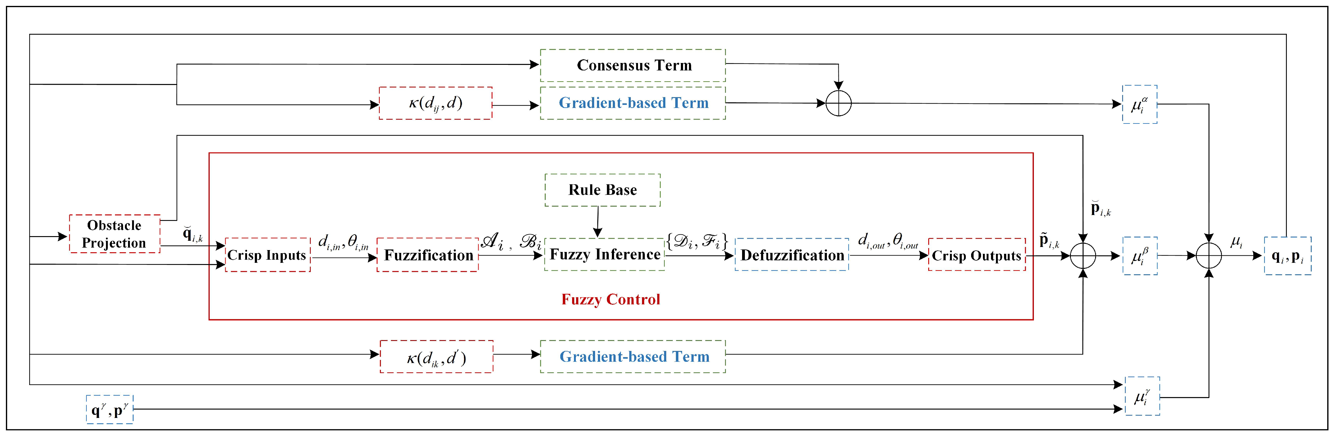
3. Proposed Algorithm

To solve Problem 1, a fuzzy flocking control (FFC) algorithm is proposed. In this algorithm, the $(\alpha ,\beta )$ interaction term ${\mathbf{u}}_i^{\beta }$, $(\alpha ,\alpha )$ interaction term ${\mathbf{u}}_i^{\alpha }$, and $(\alpha ,\gamma )$ interaction term ${\mathbf{u}}_i^{\gamma }$ are reconstructed such that the $\alpha$-agent can escape from the dynamic equilibrium, bypass obstacles, and avoid collisions. The structure of this algorithm is shown in Figure 4, and the details are described below:

3.1. Evaluate ${\mathbf{u}}_i^{\beta }$

The $(\alpha ,\beta )$ interaction term ${\mathbf{u}}_i^{\beta }$ is reconstructed by calculating the fuzzy expected velocity of $\alpha$-agent for $\beta$-agent and designing a nonnegative subsection function. When $\alpha$-agent i is trapped in dynamic equilibrium, the fuzzy expected velocity of $\alpha$-agent for $\beta$-agent is obtained by the fuzzy control method, and $\alpha$-agent i can escape from the dynamic equilibrium based on this fuzzy expected velocity. When $\alpha$-agent i is not trapped in dynamic equilibrium, the projected expected velocity of $\alpha$-agent for $\beta$-agent is obtained by Formula (14) or (15), which enables $\alpha$-agent i to bypass the obstacles. Meanwhile, the sensing radius region of $\alpha$-agent i is divided into four subregions, followed by the design of a nonnegative subsection function to adjust the attractive/repulsive potentials in these subregions, which reduces the possibility of collisions between the $\alpha$-agent and obstacles.

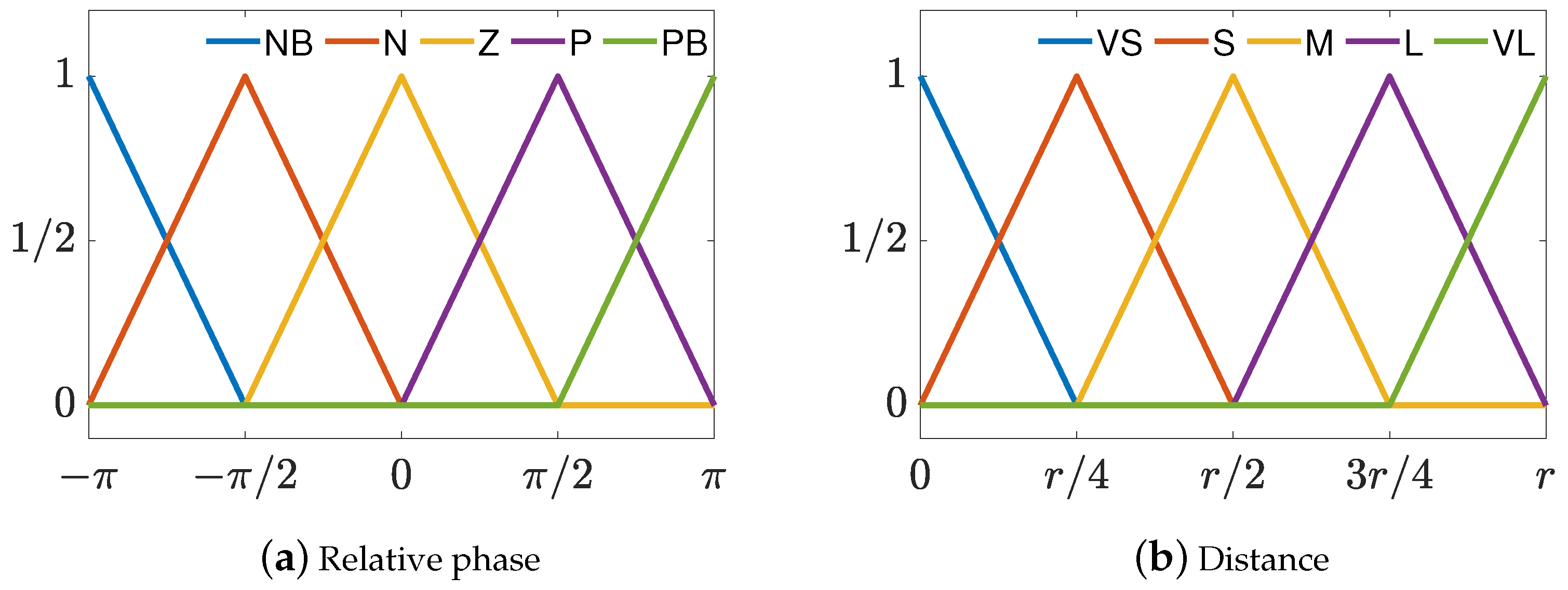
3.1.1. Fuzzy Expected Velocity Calculated by Fuzzy Control

When $\alpha$-agent i perceives the obstacles that prevent it from following the $\gamma$-agent, determine whether the position of $\alpha$-agent i satisfies Condition (21). If Condition (21) holds, $\alpha$-agent i is trapped in dynamic equilibrium. Then, the fuzzy expected velocity ${\tilde{\mathbf{p}}}_{i,k}$ of $\alpha$-agent i for $\beta$-agent k is calculated by the fuzzy control method. The core idea of this method is to encode experience-based knowledge in the form of fuzzy rules. In this method, the crisp inputs with precise values are first converted to fuzzy variable sets, which is referred to as fuzzification. Then, these fuzzy variable sets are transformed into new fuzzy variable sets by performing fuzzy inference based on the fuzzy rules. Finally, the new fuzzy variable sets are converted back to the crisp outputs, which is also referred to as defuzzification. The details of this method are described as follows:

Crisp inputs: The fuzzy expected velocity ${\tilde{\mathbf{p}}}_{i,k}$ of $\alpha$-agent i for $\beta$-agent k is equal to the distance between the current position ${\mathbf{q}}_i$ of $\alpha$-agent i and the expected position ${\tilde{\mathbf{q}}}_i$ of $\alpha$-agent i at the next time divided by the step time $\Delta t$. Thus, determining the expected position ${\tilde{\mathbf{q}}}_i$ of $\alpha$-agent i is crucial to obtain the fuzzy expected velocity ${\tilde{\mathbf{p}}}_{i,k}$. It is known that the expected position ${\tilde{\mathbf{q}}}_i$ of $\alpha$-agent i can be calculated by phase and distance. In this regard, the crisp inputs to the fuzzy control are defined as the phase and distance. To deal with phases simply, the reference coordinate system is rotated to the agent coordinate system when $\alpha$-agent i perceives the obstacles. In the agent coordinate system, the origin is the position of $\alpha$-agent i, and the direction of the x-axis points to the $\gamma$-agent. Next, the relative phase ${\theta }_{i,k}$ between $\alpha$-agent i and obstacle boundary point k can be obtained in the agent coordinate system, and ${\theta }_{i,k}={\theta }_{i,k}-2\pi$ if ${\theta }_{i,k}>\pi$. Denote ${\vartheta }_i=\{{\theta }_{i,k},k\in {\mathcal{N}}_i^{\beta }\}$ as the relative phase set of $\alpha$-agent i, $m_p$ and $m_n$ as the number of positive and negative elements in the relative phase set ${\vartheta }_i$, and $k_p$ and $k_n$ as the obstacle boundary points corresponding to the maximum and minimum values of the phases in the phase set ${\vartheta }_i$. Then, the input relative phase ${\theta }_{i,in}={\theta }_{i,k_n}$ and the input distance $d_{i,in}=\parallel {\breve{\mathbf{q}}}_{i,k_n}-{\mathbf{q}}_i\parallel$ if $m_p>m_n$, otherwise ${\theta }_{i,in}={\theta }_{i,k_p}$ and $d_{i,in}=\parallel {\breve{\mathbf{q}}}_{i,k_p}-{\mathbf{q}}_i\parallel$. Here, the input relative phase ${\theta }_{i,in}$ and the input distance $d_{i,in}$ are the crisp inputs to the fuzzy control.

Fuzzification: Let ${\vartheta }_{in}$ denote the fuzzy variable set of the input relative phase ${\theta }_{i,in}$, ${\vartheta }_{in}=\{\mathrm{NB},\mathrm{N},\mathrm{Z},\mathrm{P},\mathrm{PB}\}$, where $\mathrm{NB}$, $\mathrm{N}$, $\mathrm{Z}$, $\mathrm{P}$, and $\mathrm{PB}$ are the abbreviations of negativebig, negative, zero, positive, and positivebig. Meanwhile, let ${\mathcal{d}}_{in}$ denote the fuzzy variable set of the input distance $d_{i,in}$, ${\mathcal{d}}_{in}=\{\mathrm{VS},\mathrm{S},\mathrm{M},\mathrm{L},\mathrm{VL}\}$, where $\mathrm{VS}$, $\mathrm{S}$, $\mathrm{M}$, $\mathrm{L}$, and $\mathrm{VL}$ are the abbreviations of veryshort, short, medium, long and verylong. Then, the triangular membership functions ${\eta }_{{\mathcal{A}}_i}\left({\theta }_{i,in}\right)$ and ${\eta }_{{\mathcal{B}}_i}\left(d_{i,in}\right)$, which are shown in Figure 5a,b, are used to obtain the degrees corresponding to the linguistic variables in fuzzy variable sets ${\vartheta }_{in}$ and ${\mathcal{d}}_{in}$, respectively. Thus, the input relative phase ${\theta }_{i,in}$ and the input distance $d_{i,in}$ can be converted to the input fuzzy variable sets ${\mathcal{A}}_i$ and ${\mathcal{B}}_i$, which are given by

$$\begin{array}{cc}\hfill & {\mathcal{A}}_i=\{({\theta }_{i,in},{\eta }_{{\mathcal{A}}_i}\left({\theta }_{i,in}\right))\mid {\theta }_{i,in}\in [-\pi ,\pi ]\}\hfill \end{array}$$

(22)

$$\begin{array}{cc}\hfill & {\mathcal{B}}_i=\{(d_{i,in},{\eta }_{{\mathcal{B}}_i}\left(d_{i,in}\right))\mid d_{i,in}\in [0,r]\}\hfill \end{array}$$

(23)

Fuzzy inference: With the input fuzzy variable sets ${\mathcal{A}}_i$ and ${\mathcal{B}}_i$, it is possible to perform fuzzy inference. The fuzzy inference procedure utilizes fuzzy rules and the Mamdani algorithm [32] to create a mapping between the input fuzzy variable sets and the output fuzzy variable sets. Based on experience and intuition, the rule base is defined in

Table 1. The rule base for fuzzy control.

		${\mathcal{d}}_{\mathit{in}}$	VS	S	M	L	VL
	${\mathit{\vartheta }}_{\mathit{out}}$\${\mathcal{d}}_{\mathit{out}}$
${\mathit{\vartheta }}_{\mathit{in}}$
NB			P\S	P\S	P\L	P\VL	P\VL
N			PB\S	PB\S	PB\M	PB\VL	PB\VL
Z			P\S	P \S	P\M	P\VL	P\VL
P			NB\S	NB\S	NB\M	NB\VL	NB\VL
PB			N\S	N\S	N\L	N\VL	N\VL

, where ${\vartheta }_{out}$ denotes the fuzzy variable set of the output relative phase and ${\mathcal{d}}_{out}$ represents the fuzzy variable set of the output relative distance. It can be seen from Table 1 that the first fuzzy rule is

$$\begin{array}{cc}\hfill {\mathrm{R}}^1:& \mathrm{IF}{\theta }_{in}^1\mathrm{is}\mathrm{NB}\mathrm{AND}{d}_{in}^1\mathrm{is}\mathrm{VS}\hfill \\ & \mathrm{THEN}{\theta }_{out}^1\mathrm{is}\mathrm{P}\mathrm{AND}{d}_{out}^1\mathrm{is}\mathrm{S}\hfill \end{array}$$

where ${\theta }_{in}^1$ is a fuzzy variable of the input relative phase, $d_{in}^1$ is a fuzzy variable of the input distance, ${\theta }_{out}^1$ is a fuzzy variable of the output relative phase, and $d_{in}^1$ is a fuzzy variable of the output distance. Furthermore, the Mamdani algorithm consists of two steps: (i) assign the degree of the lth fuzzy rule, calculated by

$$\mathrm{deg}\left({\mathrm{R}}^l\right)={\eta }_{{\mathcal{A}}_i}\left({\theta }_{in}^l\right)\wedge {\eta }_{{\mathcal{B}}_i}\left(d_{in}^l\right)\wedge {\eta }_{{\mathcal{A}}_i}\left({\theta }_{out}^l\right)\wedge {\eta }_{{\mathcal{B}}_i}\left(d_{out}^l\right)$$

(24)

where $l=1,2,\dots ,N_r$, $N_r$ is the total number of fuzzy rules in the rule base, and ∧ denotes the “min” operation, and (ii) let ${\eta }_o^l$ be the degree of the lth fuzzy rule in the output fuzzy subset for the input $\{{\theta }_{in}^l,d_{in}^l\}$, given by

$${\eta }_o^l={\eta }_{{\mathcal{A}}_i}\left({\theta }_{in}^l\right)\wedge {\eta }_{{\mathcal{B}}_i}\left(d_{in}^l\right)$$

(25)

then the output fuzzy variable sets $\{{\mathcal{D}}_i,{\mathcal{F}}_i\}$ are the synthesis of ${\eta }_o^l$ and $\mathrm{deg}\left({\mathrm{R}}^l\right)$, obtained by

$$\{{\mathcal{D}}_i,{\mathcal{F}}_i\}=\vee [{\eta }_o^l\wedge \mathrm{deg}\left({\mathrm{R}}^l\right)]$$

(26)

where ∨ denotes the “max” operation.

Defuzzification: Let ${\theta }_{i,out}$ be the output relative phase, and $d_{i,out}$ be the output distance. Then, the output fuzzy variable sets can be converted into a series of subregions using the membership functions ${\eta }_{{\mathcal{A}}_i}\left({\theta }_{i,out}\right)$ and ${\eta }_{{\mathcal{B}}_i}\left(d_{i,out}\right)$. In addition, let $m_{{\mathcal{A}}_i}$ be the number of subregions obtained by the membership functions ${\eta }_{{\mathcal{A}}_i}\left({\theta }_{i,out}\right)$, and ${\theta }_{i,out}^g$ be the phase in the center of subregion g. Similarly, let $m_{{\mathcal{B}}_i}$ be the number of subregions obtained by the membership functions ${\eta }_{{\mathcal{B}}_i}\left(d_{i,out}\right)$, and $d_{i,out}^g$ be the distance in the center of subregion g. Then, the output relative phase ${\theta }_{i,out}$ and the output distance $d_{i,out}$ are obtained by calculating the center of gravity as follows:

$$\begin{array}{cc}\hfill {\theta }_{i,out}& ={\displaystyle \frac{{\sum }_{g=1}^{m_{{\mathcal{A}}_i}}{\theta }_{i,out}^g·{\eta }_{{\mathcal{A}}_i}\left({\theta }_{i,out}^g\right)}{{\sum }_{g=1}^{m_{{\mathcal{A}}_i}}\left({\eta }_{{\mathcal{A}}_i}\left({\theta }_{i,out}^g\right)\right)}}\hfill \end{array}$$

(27)

$$\begin{array}{cc}\hfill d_{i,out}& ={\displaystyle \frac{{\sum }_{g=1}^{m_{{\mathcal{B}}_i}}{d}_{i,out}^g·{\eta }_{{\mathcal{B}}_i}\left(d_{i,out}^g\right)}{{\sum }_{g=1}^{m_{{\mathcal{B}}_i}}\left({\eta }_{{\mathcal{B}}_i}\left(d_{i,out}^g\right)\right)}}\hfill \end{array}$$

(28)

Crisp outputs: The expected position ${\tilde{\mathbf{q}}}_i$ of $\alpha$-agent i is calculated by

$${\tilde{\mathbf{q}}}_i={\mathbf{q}}_i+d_{i,out}\xi \left({\theta }_{i,out}\right)$$

(29)

where

$$\begin{array}{cc}\hfill & {\theta }_{i,out}=[{\theta }_{i,az,out},{\theta }_{i,el,out}]\hfill \end{array}$$

(30)

$$\begin{array}{cc}\hfill & \xi \left({\theta }_{i,out}\right)={\xi }_1\left({\theta }_{i,el,out}\right)\odot {\xi }_2\left({\theta }_{i,az,out}\right)\hfill \end{array}$$

(31)

$$\begin{array}{cc}\hfill & {\xi }_1\left({\theta }_{i,el,out}\right)=[\cos {\theta }_{i,el,out},\cos {\theta }_{i,el,out},1]\hfill \end{array}$$

(32)

$$\begin{array}{cc}\hfill & {\xi }_2\left({\theta }_{i,az,out}\right)=[\sin {\theta }_{i,az,out},\cos {\theta }_{i,az,out},\sin {\theta }_{i,az,out}]\hfill \end{array}$$

(33)

and ${\theta }_{i,az,out}$ is the relative azimuth, ${\theta }_{i,el,out}$ is the relative elevation, and ⊙ is the Hadamard product. Note that ${\theta }_{i,el,out}=0$ if $\alpha$-agent i is in two-dimensional Euclidean space. Thus, the fuzzy expected velocity ${\tilde{\mathbf{p}}}_{i,k}$ of $\alpha$-agent i for $\beta$-agent k is calculated by

$${\tilde{\mathbf{p}}}_{i,k}={\displaystyle \frac{{\tilde{\mathbf{q}}}_i-{\mathbf{q}}_i}{\Delta t}}$$

(34)

Substituting Formula (29) into Formula (34), we have

$${\tilde{\mathbf{p}}}_{i,k}={\displaystyle \frac{d_{i,out}\xi \left({\theta }_{i,out}\right)}{\Delta t}}$$

(35)

3.1.2. Nonnegative Subsection Function

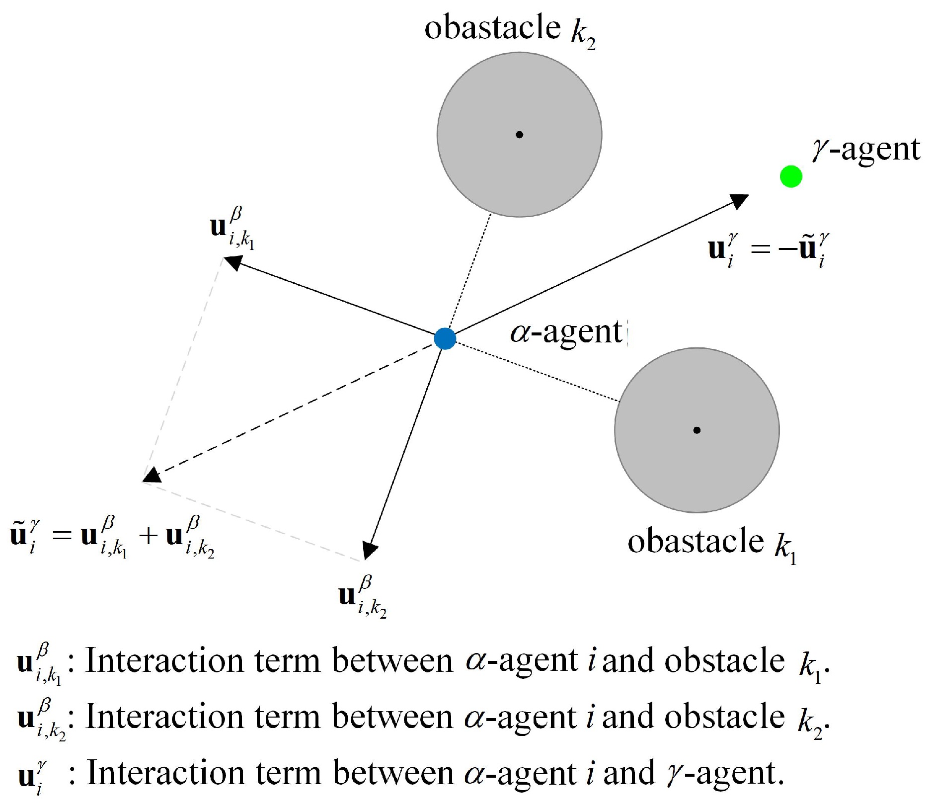
When the distance between $\alpha$-agent i and $\beta$-agent k is less than $d^{\prime }$, the repulsion enables their separation. However, the continuous reduction in distance between $\alpha$-agent i and $\beta$-agent k presents a collision risk. Early warning can be used to reduce the collision risk [33]. Hence, we define $d_c$ as the minimum early-warning distance, and the collision region as the area within a distance $d_c$ from $\alpha$-agent i. Furthermore, maintaining a strict distance $d^{\prime }$ between $\alpha$-agent i and $\beta$-agent k is difficult in practice. To solve this problem, we define ${ϵ}_2$ as the disturbance factor, and the alignment region as the area whose distance from $\alpha$-agent i is greater than $d^{\prime }-{ϵ}_2$ and less than $d^{\prime }+{ϵ}_2$. Thus, the sensing radius region of $\alpha$-agent i is divided into four subregions, as shown in Figure 6. It is known that the attractive/repulsive potential can achieve separation, alignment, and attraction between $\alpha$-agent i and $\beta$-agent k [10]. Here, a nonnegative subsection function $\kappa (d_{i,k},d^{\prime })$ is designed to adjust the attractive/repulsive potential in these four subregions, given by

$$\kappa (d_{i,k},d^{\prime })=\left\{\begin{array}{cc}{\tau }_1,\hfill & d_{i,k}\in (0,d_c),\hfill \\ {\tau }_2,\hfill & d_{i,k}\in [d_c,d^{\prime }-{ϵ}_2],\hfill \\ {\tau }_3,\hfill & d_{i,k}\in (d^{\prime }-{ϵ}_2,d^{\prime }+{ϵ}_2],\hfill \\ {\tau }_4,\hfill & d_{i,k}\in (d^{\prime }+{ϵ}_2,r],\hfill \end{array}\right.$$

(36)

where ${\tau }_1$, ${\tau }_2$, ${\tau }_3$, and ${\tau }_4$ are the weights, $d_c=d_{\mathrm{safe}}+2p_{i,m}\Delta t$, $d_{\mathrm{safe}}$ is the minimum safe distance for avoiding collisions since the size of $\alpha$-agent i cannot be ignored in practice, ${ϵ}_2$ is a constant, $d_{i,k}=\parallel {\breve{\mathbf{q}}}_{i,k}-{\mathbf{q}}_i\parallel$, and $d_{i,k}\in (d^{\prime }-{ϵ}_2,d^{\prime }+{ϵ}_2]$ is the desired distance for collision avoidance.

With the fuzzy expected velocity ${\tilde{\mathbf{p}}}_{i,k}$ of $\alpha$-agent i for $\beta$-agent k and the nonnegative subsection function $\kappa (d_{i,k},d^{\prime })$, the $(\alpha ,\beta )$ interaction term ${\mathbf{u}}_i^{\beta }$ is reconstructed as

$$\begin{array}{cc}\hfill {\mathbf{u}}_i^{\beta }=& -c_1^{\beta }\sum _{k\in {\mathcal{N}}_i^{\beta }}\kappa (d_{i,k},d^{\prime }){\nabla }_{{\mathbf{q}}_i}{\psi }^{\beta }\left({\parallel {\breve{\mathbf{q}}}_{i,k}-{\mathbf{q}}_i\parallel }_{\sigma }\right)+(1-h_i)c_2^{\beta }\sum _{k\in {\mathcal{N}}_i^{\beta }}{b}_{i,k}\left(\mathbf{q}\right)({\breve{\mathbf{p}}}_{i,k}-{\mathbf{p}}_i)\hfill \\ & +h_i{c}_3^{\beta }\sum _{k\in {\mathcal{N}}_i^{\beta }}{b}_{i,k}\left(\mathbf{q}\right)({\tilde{\mathbf{p}}}_{i,k}-{\mathbf{p}}_i)\hfill \end{array}$$

(37)

where $c_3^{\beta }$ is the feedback gain, $d_{i,k}$ is the distance between $\alpha$-agent i and $\beta$-agent k, $d_{i,k}=\parallel {\breve{\mathbf{q}}}_{i,k}-{\mathbf{q}}_i\parallel$, ${\breve{\mathbf{q}}}_{i,k}$ is the projected expected position of $\alpha$-agent i for $\beta$-agent k, ${\breve{\mathbf{p}}}_{i,k}$ is the projected expected velocity of $\alpha$-agent i for $\beta$-agent k, and $h_i=1$ if $\alpha$-agent i is trapped in dynamic equilibrium, otherwise $h_i=0$. Here, the projected expected position ${\breve{\mathbf{q}}}_{i,k}$ and projected expected velocity ${\breve{\mathbf{p}}}_{i,k}$ are calculated by Formulas (14) and (15).

3.2. Evaluate ${\mathbf{u}}_i^{\alpha }$

With the nonnegative subsection function $\kappa (d_{ij},d)$, the $(\alpha ,\alpha )$ interaction term ${\mathbf{u}}_i^{\alpha }$ is reconstructed as

$$\begin{array}{c}\hfill {\mathbf{u}}_i^{\alpha }=-c_1^{\alpha }\sum _{j\in {\mathcal{N}}_i^{\alpha }}\kappa (d_{ij},d){\nabla }_{{\mathbf{q}}_i}{\psi }^{\alpha }\left({\parallel {\mathbf{q}}_j-{\mathbf{q}}_i\parallel }_{\sigma }\right)+c_2^{\alpha }\sum _{j\in {\mathcal{N}}_i^{\alpha }}{a}_{ij}\left(\mathbf{q}\right)({\mathbf{p}}_j-{\mathbf{p}}_i)\end{array}$$

(38)

where $d_{ij}$ is the distance between $\alpha$-agents i and j, $d_{ij}=\parallel {\mathbf{q}}_j-{\mathbf{q}}_i\parallel$.

3.3. Evaluate ${\mathbf{u}}_i^{\gamma }$

To increase the attractiveness of the $\gamma$-agent to $\alpha$-agent i, the $(\alpha ,\gamma )$ interaction term ${\mathbf{u}}_i^{\gamma }$ is reconstructed as

$$\begin{array}{c}\hfill {\mathbf{u}}_i^{\gamma }=-c_1^{\gamma }({\mathbf{q}}_i-{\mathbf{q}}^{\gamma })-c_2^{\gamma }({\mathbf{p}}_i-{\mathbf{p}}^{\gamma })\end{array}$$

(39)

Using Formulas (37)–(39) and (13), the control input ${\mathbf{u}}_i$ for $\alpha$-agent i can be obtained. In summary, the details of the FFC algorithm are described in Algorithm 1.

Algorithm 1 FFC algorithm

Input: Runtime $T_m$, r, d, $d^{\prime }$, ${ϵ}_1$, ${ϵ}_2$, h, a, b, $c_1^{\alpha }$, $c_2^{\alpha }$, $c_1^{\beta }$, $c_2^{\beta }$, $c_3^{\beta }$, $c_1^{\gamma }$, $c_2^{\gamma }$, m, $\Delta t$, $\lambda$, $p_{i,m}$, $d_{\mathrm{safe}}$, ${\tau }_1$, ${\tau }_2$, ${\tau }_3$, ${\tau }_4$. Initialization: ${\mathbf{q}}^{\gamma }$, ${\mathbf{p}}^{\gamma }$, ${\mathbf{q}}_i$, ${\mathbf{p}}_i$, $t=0$. Iteration: 1: If $\parallel {\breve{\mathbf{q}}}_{i,k}-{\mathbf{q}}_i\parallel <r$ and (21) is true, $h_i=1$ and calculate ${\tilde{\mathbf{p}}}_{i,k}$ by fuzzy control: (1) Obtain ${\theta }_{i,in}$ and $d_{i,in}$ in the agent coordinate system. (2) Calculate ${\mathcal{A}}_i$ using (22) and ${\mathcal{B}}_i$ using (23). (3) Calculate $\{{\mathcal{D}}_i,{\mathcal{F}}_i\}$ using (26). (4) Calculate ${\theta }_{i,out}$ using (27) and $d_{i,out}$ using (28). (5) Calculate ${\tilde{\mathbf{p}}}_{i,k}$ using (34). Otherwise, $h_i=0$ and calculate ${\breve{\mathbf{p}}}_{i,k}$ using (14) or (15). 2: Calculate $\kappa (d_{ij},d)$ and $\kappa (d_{i,k},d^{\prime })$ using (36). 3: Evaluate ${\mathbf{u}}_i^{\beta }$ using (37). 4: Evaluate ${\mathbf{u}}_i^{\alpha }$ using (38). 5: Evaluate ${\mathbf{u}}_i^{\gamma }$ using (39). 6: Evaluate ${\mathbf{u}}_i$ using (13), update ${\mathbf{q}}_i$ using (1), and output ${\mathbf{q}}_i$ and ${\mathbf{p}}_i$. 7: If $t>T_m$, terminate the iteration. Otherwise, set $t=t+\Delta t$ and return to step 1. Output: ${\mathbf{q}}_i$, ${\mathbf{p}}_i$.

4. Properties Analysis of FFC Algorithm

Denote ${\Phi }^{\alpha }\left(t\right)$ as the total potential energy between the $\alpha$-agents, ${\Phi }^{\beta }\left(t\right)$ as the total potential energy between the $\alpha$-agent and $\beta$-agent, ${\Phi }_p^{\gamma }\left(t\right)$ as the total potential energy between the $\alpha$-agent and $\gamma$-agent, and ${\Phi }_k^{\gamma }\left(t\right)$ as the kinetic energy between the $\alpha$-agent and $\gamma$-agent. Then, the total energy $E\left(t\right)$ can be defined by

$$E\left(t\right)={\Phi }^{\alpha }\left(t\right)+{\Phi }^{\beta }\left(t\right)+{\Phi }_p^{\gamma }\left(t\right)+{\Phi }_k^{\gamma }\left(t\right)$$

(40)

where

$$\begin{array}{cc}\hfill {\Phi }^{\alpha }\left(t\right)& ={\displaystyle \frac{c_1^{\alpha }}{2}}\sum _{i=1}^N\sum _{j\in {\mathcal{N}}_i^{\alpha }}\kappa (d_{ij},d){\psi }^{\alpha }(\parallel {\mathbf{q}}_j-{\mathbf{q}}_i{\parallel }_{\sigma })\hfill \end{array}$$

(41)

$$\begin{array}{cc}\hfill {\Phi }^{\beta }\left(t\right)& =c_1^{\beta }\sum _{i=1}^N\sum _{k\in {\mathcal{N}}_i^{\beta }}\kappa (d_{i,k},d^{\prime }){\psi }^{\beta }(\parallel {\breve{\mathbf{q}}}_{i,k}-{\mathbf{q}}_i{\parallel }_{\sigma })\hfill \end{array}$$

(42)

$$\begin{array}{cc}\hfill {\Phi }_p^{\gamma }\left(t\right)& ={\displaystyle \frac{c_1^{\gamma }}{2}}\sum _{i=1}^N{({\mathbf{q}}_i-{\mathbf{q}}^{\gamma })}^{\mathrm{T}}({\mathbf{q}}_i-{\mathbf{q}}^{\gamma })\hfill \end{array}$$

(43)

$$\begin{array}{cc}\hfill {\Phi }_k^{\gamma }\left(t\right)& ={\displaystyle \frac{1}{2}}\sum _{i=1}^N{({\mathbf{p}}_i-{\mathbf{p}}^{\gamma })}^{\mathrm{T}}({\mathbf{p}}_i-{\mathbf{p}}^{\gamma })\hfill \end{array}$$

(44)

Theorem 1.

Consider a group of N α-agents with its motion model (1). The control inputs acting on these α-agents are obtained by Formulas (13) and (37)–(39). Assume that the γ-agent is static, i.e., ${\mathbf{p}}^{\gamma }=0$. Furthermore, assume that the initial total energy $E\left(0\right)$ is finite. Then, $\parallel {\mathbf{q}}_i-{\mathbf{q}}^{\gamma }\parallel \le \sqrt{2E\left(0\right)/c_1^{\gamma }},i=1,2,\dots ,N$ holds for all $t\ge 0$.

Proof. 

Calculating the first order derivative of the total energy $E\left(t\right)$, we can obtain

$${\displaystyle \frac{dE\left(t\right)}{dt}}={\displaystyle \frac{d{\Phi }^{\alpha }\left(t\right)}{dt}}+{\displaystyle \frac{d{\Phi }^{\beta }\left(t\right)}{dt}}+{\displaystyle \frac{d{\Phi }_p^{\gamma }\left(t\right)}{dt}}+{\displaystyle \frac{d{\Phi }_k^{\gamma }\left(t\right)}{dt}}$$

(45)

where

$$\begin{array}{cc}\hfill {\displaystyle \frac{d{\Phi }^{\alpha }\left(t\right)}{dt}}& =c_1^{\alpha }\sum _{i=1}^N\sum _{j\in {\mathcal{N}}_i^{\alpha }}\kappa (d_{ij},d){\left({\mathbf{p}}_i\right)}^{\mathrm{T}}{\nabla }_{{\mathbf{q}}_i}{\psi }^{\alpha }(\parallel {\mathbf{q}}_j-{\mathbf{q}}_i{\parallel }_{\sigma })\hfill \end{array}$$

(46)

$$\begin{array}{cc}\hfill {\displaystyle \frac{d{\Phi }^{\beta }\left(t\right)}{dt}}& =c_1^{\beta }\sum _{i=1}^N\sum _{k\in {\mathcal{N}}_i^{\beta }}\kappa (d_{i,k},d^{\prime }){\left({\mathbf{p}}_i\right)}^{\mathrm{T}}{\nabla }_{{\mathbf{q}}_i}{\psi }^{\beta }(\parallel {\breve{\mathbf{q}}}_{i,k}-{\mathbf{q}}_i{\parallel }_{\sigma })\hfill \end{array}$$

(47)

$$\begin{array}{cc}\hfill {\displaystyle \frac{d{\Phi }_p^{\gamma }\left(t\right)}{dt}}& =c_1^{\gamma }\sum _{i=1}^N{\left({\mathbf{p}}_i\right)}^{\mathrm{T}}({\mathbf{q}}_i-{\mathbf{q}}^{\gamma })\hfill \end{array}$$

(48)

$$\begin{array}{cc}\hfill {\displaystyle \frac{d{\Phi }_k^{\gamma }\left(t\right)}{dt}}& =\sum _{i=1}^N{\left({\mathbf{p}}_i\right)}^{\mathrm{T}}{\mathbf{u}}_i\hfill \end{array}$$

(49)

Formulas (13), (37)–(39) and (45) can be rewritten as

$$\begin{array}{cc}\hfill {\displaystyle \frac{dE\left(t\right)}{dt}}=& -c_2^{\alpha }\sum _{i=1}^N\sum _{j\in {\mathcal{N}}_i^{\alpha }}{a}_{ij}\left(\mathbf{q}\right){\left({\mathbf{p}}_i\right)}^{\mathrm{T}}({\mathbf{p}}_i-{\mathbf{p}}_j)-c_2^{\beta }\sum _{i=1}^N\sum _{k\in {\mathcal{N}}_i^{\beta }}(1-h_i)b_{i,k}\left(\mathbf{q}\right){\left({\mathbf{p}}_i\right)}^{\mathrm{T}}({\mathbf{p}}_i-{\breve{\mathbf{p}}}_{i,k})\hfill \\ & -c_3^{\beta }\sum _{i=1}^N\sum _{k\in {\mathcal{N}}_i^{\beta }}{h}_i{b}_{i,k}\left(\mathbf{q}\right){\left({\mathbf{p}}_i\right)}^{\mathrm{T}}({\mathbf{p}}_i-{\tilde{\mathbf{p}}}_{i,k})-c_2^{\gamma }\sum _{i=1}^N{\left({\mathbf{p}}_i\right)}^{\mathrm{T}}{\mathbf{p}}_i\hfill \end{array}$$

(50)

Let ${\mathbf{v}}_1={[{\mathbf{p}}_1^{\mathrm{T}}\cdots {\mathbf{p}}_N^{\mathrm{T}}]}^{\mathrm{T}}$, ${\mathbf{v}}_2={[{\breve{\mathbf{p}}}_{1,k}^{\mathrm{T}}\cdots {\breve{\mathbf{p}}}_{N,k}^{\mathrm{T}}]}^{\mathrm{T}}$, ${\mathbf{v}}_3={[{\tilde{\mathbf{p}}}_{1,k}^{\mathrm{T}}\cdots {\tilde{\mathbf{p}}}_{N,k}^{\mathrm{T}}]}^{\mathrm{T}}$, and ${\mathbf{v}}^{\prime }=[{\mathbf{v}}_1,{\mathbf{v}}_2,{\mathbf{v}}_3]$. In addition, let ${\mathbf{F}}_A$ be a diagonal matrix whose ith diagonal element is given by $f_a(i,i)={\sum }_{j\in {\mathcal{N}}_i^{\alpha }}{a}_{ij}\left(\mathbf{q}\right)$, $\mathbf{A}$ be a adjacency matrix whose $(i,j)$th element is $a_{ij}\left(\mathbf{q}\right)$, ${\mathbf{L}}_A$ be a Laplacian matrix given by ${\mathbf{L}}_A={\mathbf{F}}_A-\mathbf{A}$, ${\mathbf{F}}_B$ be a diagonal matrix whose ith diagonal element is given by $f_b(i,i)={\sum }_{k\in {\mathcal{N}}_i^{\beta }}(1-h_i)b_{i,k}\left(\mathbf{q}\right)$, $\mathbf{B}$ be a adjacency matrix whose $(i,j)$th element is $(1-h_i)b_{i,k}\left(\mathbf{q}\right)$, ${\mathbf{F}}_C$ be a diagonal matrix whose ith diagonal element is given by $f_c(i,i)={\sum }_{k\in {\mathcal{N}}_i^{\beta }}{h}_i{b}_{i,k}\left(\mathbf{q}\right)$, and $\mathbf{C}$ be a adjacency matrix whose $(i,j)$th element is $h_i{b}_{i,k}\left(\mathbf{q}\right)$. This introduces a matrix as follows

$$\left.\mathbf{R}=\left(\begin{array}{ccc}{c}_2^{\alpha }{\mathbf{L}}_A+c_2^{\beta }{\mathbf{F}}_B+c_3^{\beta }{\mathbf{F}}_C+c_2^{\gamma }{\mathbf{I}}_N& {\mathbf{F}}_0& {\mathbf{F}}_0\\ -c_2^{\beta }\mathbf{B}& {\mathbf{F}}_0& {\mathbf{F}}_0\\ -c_3^{\beta }\mathbf{C}& {\mathbf{F}}_0& {\mathbf{F}}_0\end{array}\right.\right)$$

(51)

Formula (50) can be equivalently reformulated as

$${\displaystyle \frac{dE\left(t\right)}{dt}}=-{\left({\mathbf{v}}^{\prime }\right)}^{\mathrm{T}}(\mathbf{R}\otimes {\mathbf{I}}_n){\mathbf{v}}^{\prime }$$

(52)

where ${\mathbf{I}}_N\in {\mathbb{R}}^{N\times N}$ and ${\mathbf{I}}_n\in {\mathbb{R}}^{n\times n}$ are the identity matrices, ${\mathbf{F}}_0\in {\mathbb{R}}^{N\times N}$ is the zero matrix, and ⊗ is the Kronecker product.

Since $c_2^{\alpha }>0$, $c_2^{\beta }>0$, $c_3^{\beta }>0$, $c_2^{\gamma }>0$, and ${\mathbf{L}}_A$, ${\mathbf{F}}_B$, ${\mathbf{F}}_C$ are positive semidefinite matrices, then $\mathbf{R}$ is a positive semidefinite matrix. Thus, we have ${\left({\mathbf{v}}^{\prime }\right)}^{\mathrm{T}}(\mathbf{R}\otimes {\mathbf{I}}_n){\mathbf{v}}^{\prime }\ge 0$ and ${\displaystyle \frac{dE\left(t\right)}{dt}}\le 0$. It can be seen that the total energy $E\left(t\right)$ is a nonincreasing function, i.e., $E\left(t\right)\le E\left(0\right)$ for all $t\ge 0$. According to Formula (40), we have ${\Phi }_p^{\gamma }\left(t\right)\le E\left(0\right)$. Therefore, $\parallel {\mathbf{q}}_i-{\mathbf{q}}^{\gamma }\parallel \le \sqrt{2E\left(0\right)/c_1^{\gamma }},i=1,2,\dots N$ holds for all $t\ge 0$.

□

Theorem 2.

Consider a group of N α-agents satisfying Theorem 1. Then, there is no collision between the α-agent and objects (e.g., other α-agents or obstacles).

Proof. 

Assume that there are ${\overline{e}}_1$ collisions between $\alpha$-agents and ${\overline{e}}_2$ collisions between the $\alpha$-agent and obstacles occurring at time t, ${\overline{e}}_1+{\overline{e}}_2=\overline{e}$. Then, we have

$$\begin{array}{cc}\hfill E\left(t\right)& \ge {\overline{e}}_1{\psi }^{\alpha }\left(0\right)+{\overline{e}}_2{\psi }^{\beta }\left(0\right)\hfill \\ & \ge \left(\overline{e}\right)\min \{{\psi }^{\alpha }\left(0\right),{\psi }^{\beta }\left(0\right)\}\hfill \end{array}$$

(53)

It is known from Formulas (9) and (10) that the pairwise attractive/repulsive potential ${\psi }^{\alpha }\left(0\right)$ and ${\psi }^{\beta }\left(0\right)$ tend to infinity. That is, $E\left(t\right)\ge E\left(0\right)$ if $\overline{e}\ne 0$. This contradicts the proof that $E\left(t\right)$ is a nonincreasing function. Hence, $\overline{e}=0$, i.e., there is no collision between the $\alpha$-agent and objects. □

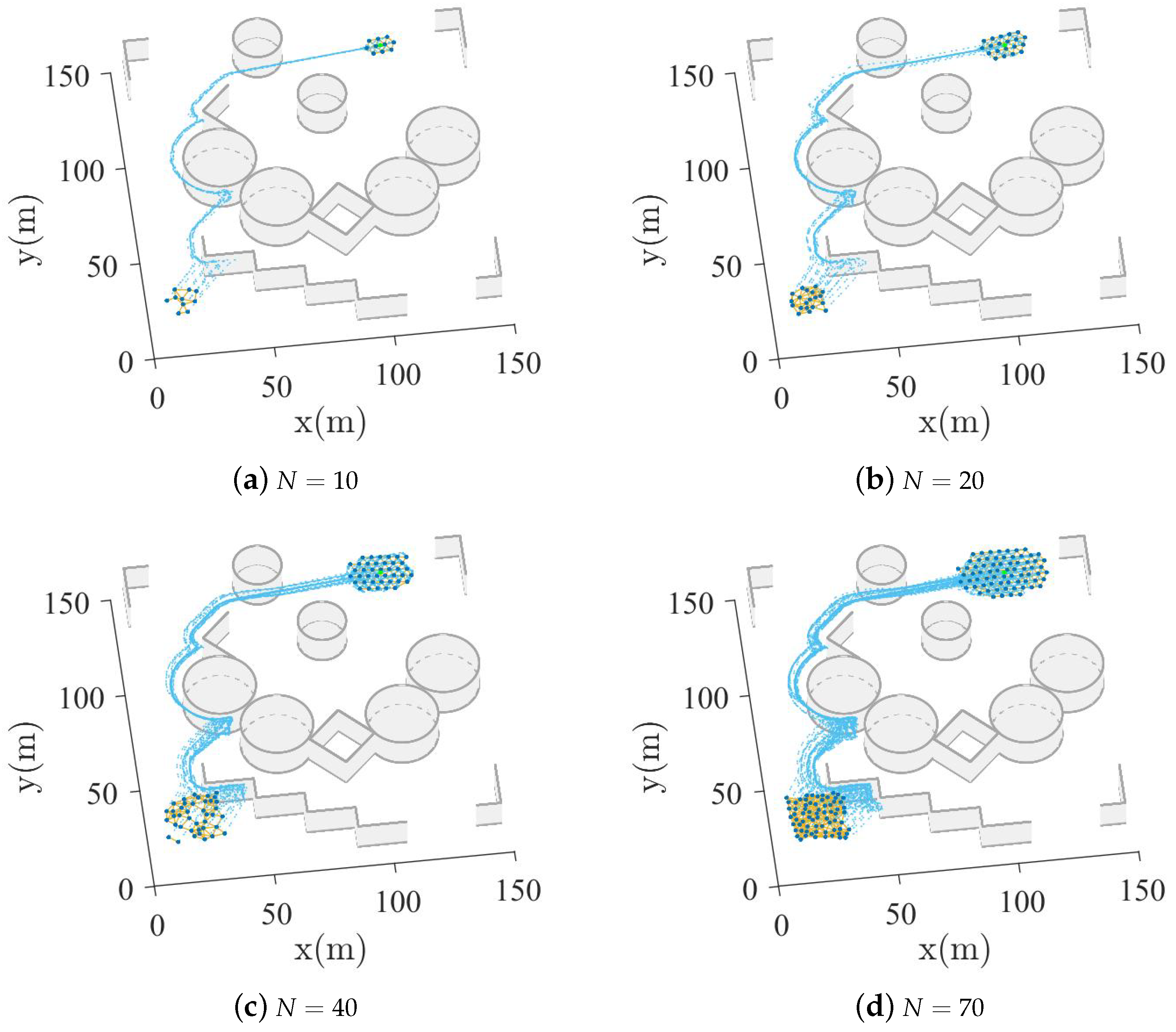
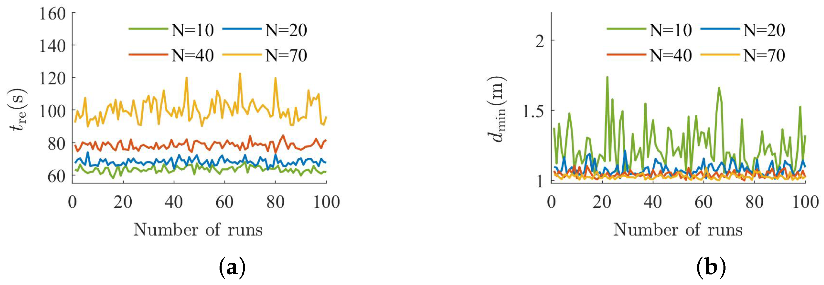
5. Experimental Results and Discussion

In this section, three experiments are undertaken to demonstrate the effectiveness of the proposed FFC algorithm, including the spherical or wall obstacle scenario, spherical and wall obstacle combination scenario, and complex obstacle scenario experiments. All experiments are carried out via Matlab R2022b on the DELL PC, which has a $3.2$ GHz i9-14900K CPU and 32 GB of memory. In addition, the OSF algorithm [10] is selected for comparison with the FFC algorithm. Meanwhile, denote $d_{\alpha \gamma }$ as the distance between the center of the $\alpha$-agents and the $\gamma$-agent, $d_{\min }$ as the minimum distance between the $\alpha$-agent and objects, and $t_{\mathrm{re}}$ as the time taken for all $\alpha$-agents to bypass obstacles and re-aggregate near the $\gamma$-agent. The distances $d_{\alpha \gamma }$ and $d_{\min }$, and the time $t_{\mathrm{re}}$, are used to evaluate the performance of the OSF and FFC algorithms.

The parameters of the OSF and FFC algorithms are shown in

Table 2. Experimental parameters.

Experiments	Parameters
A, B, and C	$c_1^{\alpha }=c_2^{\alpha }=c_1^{\beta }=c_2^{\beta }=c_3^{\beta }=c_1^{\gamma }=c_2^{\gamma }=1$,
	$d=d^{\prime }=4$, $r=6$, $a=2$, $b=20$, $\lambda =0.8$,
	$h=0.2$, $p_{i,m}=5\mathrm{m}/\mathrm{s}$, ${ϵ}_1=0.5$, ${ϵ}_2=0.5$,
	${\tau }_1=$ 10,000, ${\tau }_2=100$, ${\tau }_3=10$, ${\tau }_4=0.1$,
	$d_{\mathrm{safe}}=1\mathrm{m}$, $m=10$, $\Delta t=0.1 \mathrm{s}$, $T_m=300$.

. Specifically, the feedback gains satisfy $c_1^{\alpha }>0$, $c_2^{\alpha }>0$, $c_1^{\beta }>0$, $c_2^{\beta }>0$, $c_3^{\beta }>0$, $c_1^{\gamma }>0$, and $c_2^{\gamma }>0$. If the values of these feedback gains are identical, it can better capture the combined effects of the interaction terms $(\alpha ,\beta )$, $(\alpha ,\alpha )$, and $(\alpha ,\gamma )$. Moreover, if the values of these feedback gains are high, the velocity of the $\alpha$-agent may tend to saturation. The weights ${\tau }_2$, ${\tau }_3$, and ${\tau }_4$ satisfy ${\tau }_2\ge {\tau }_3\ge {\tau }_4\ge 0$. In addition, the weight ${\tau }_1$ is crucial for early warning and should satisfy ${\tau }_1\gg {\tau }_2$.

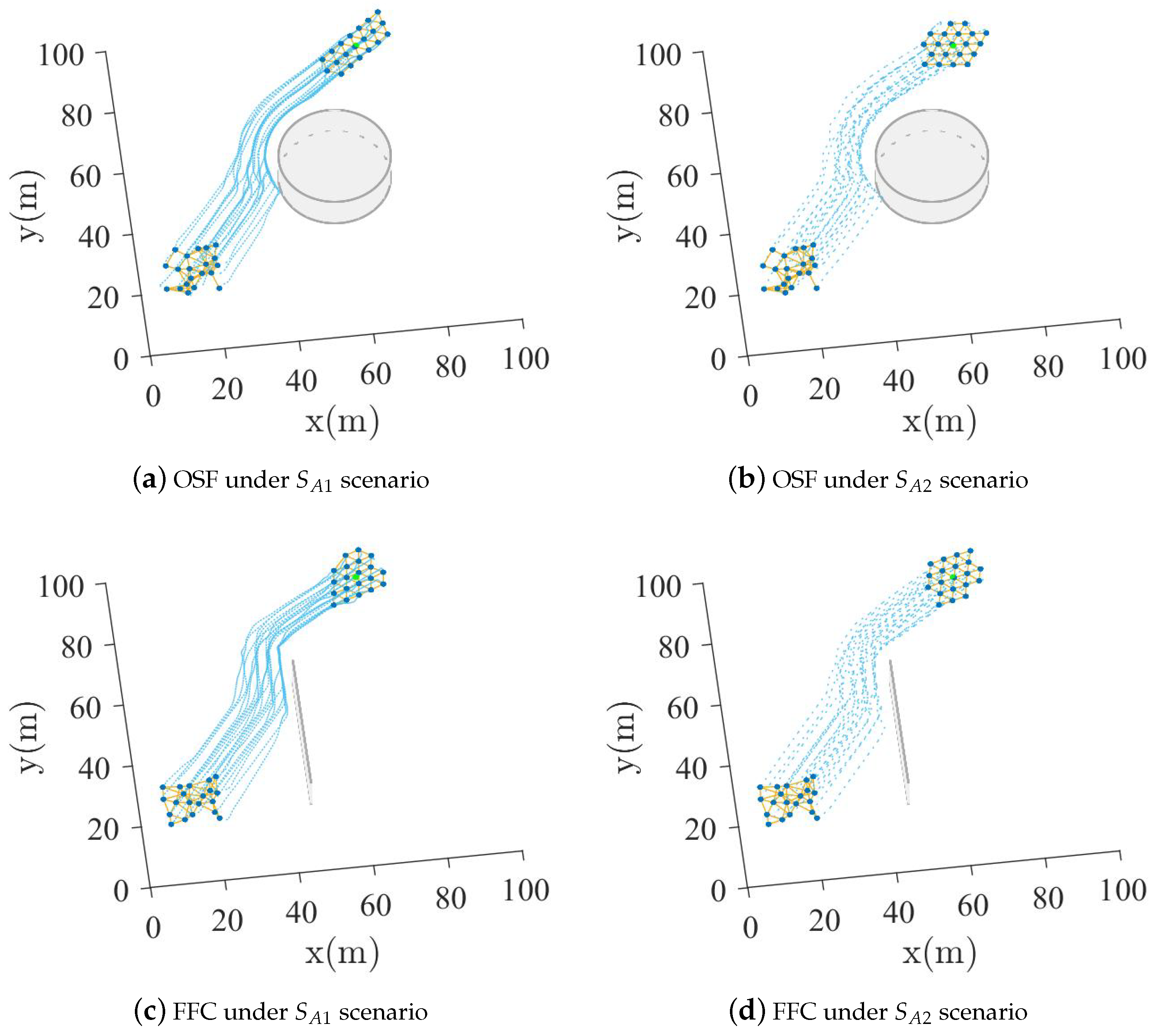
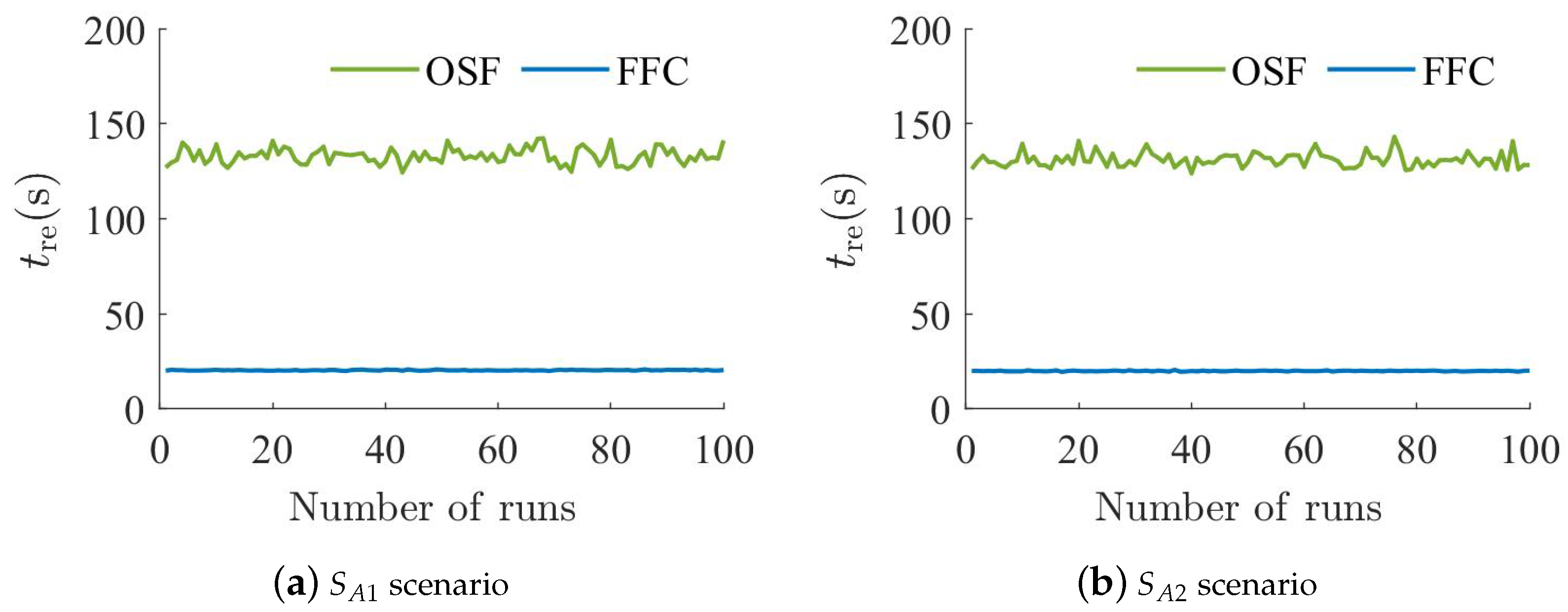
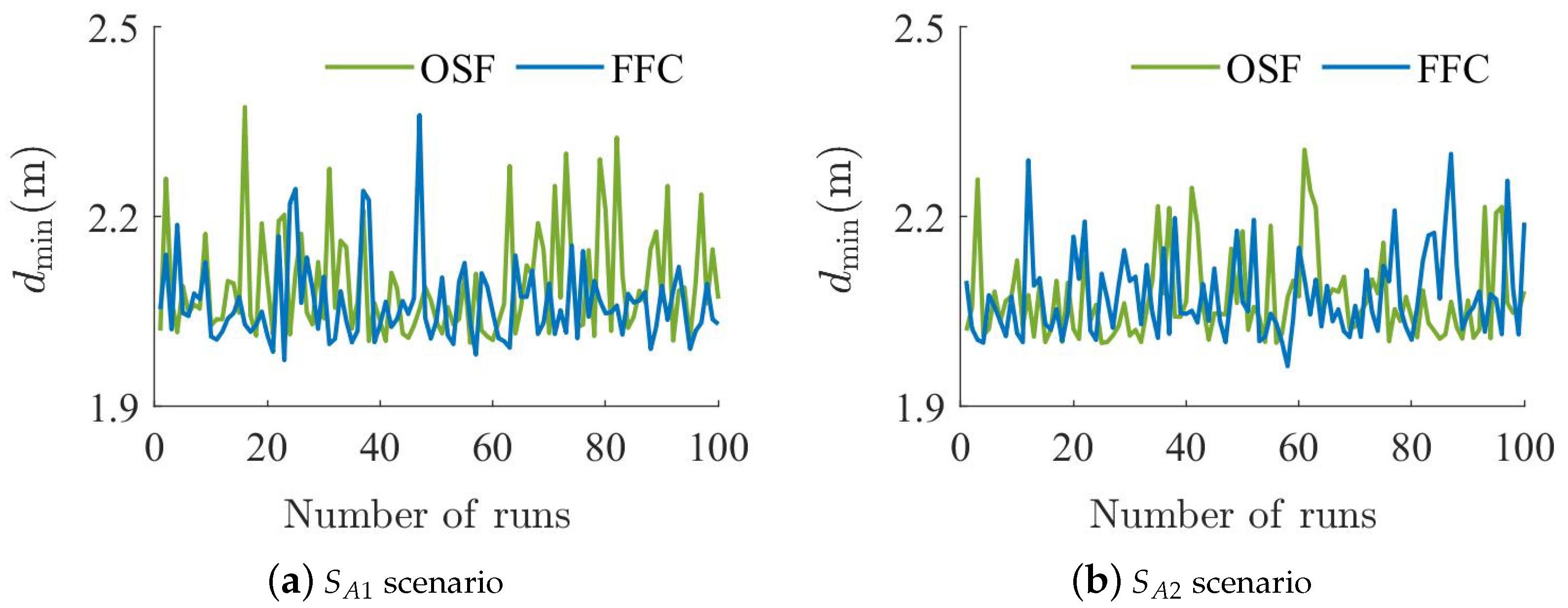
5.1. Spherical or Wall Obstacle Scenario Experiment

In this experiment, two obstacle scenarios are selected as follows:

$S_{A1}$:

There is a spherical obstacle of radius 15 at coordinates $[55, 45]$.

$S_{A2}$:

There is a wall obstacle of length 30 at coordinates $[45, 55]$.

The number of $\alpha$-agents is $N=20$, the initial positions of these $\alpha$-agents are selected randomly from ${[5, 20]}^2$, and the initial velocities of these $\alpha$-agents are selected randomly from ${[0, 2]}^2$. In addition, the initial position of the virtual $\gamma$-agent is $[65, 80]$, and the initial velocity of the virtual $\gamma$-agent is zero.

The visual comparison of the two algorithms is shown in Figure 7. It can be seen that the two algorithms can enable all $\alpha$-agents to bypass spherical or wall obstacles and follow the $\gamma$-agent. Furthermore, the quantitative comparison of the two algorithms over 100 runs is shown in Figure 8 and Figure 9. It can be seen from Figure 8 that the time taken for all $\alpha$-agents to bypass obstacles and re-aggregate near the $\gamma$-agent is reduced compared to the OSF algorithm, which indicates that the FFC algorithm enables $\alpha$-agents to bypass the obstacle faster. Meanwhile, it can be seen from Figure 9 that the minimum distance of the two algorithms between the $\alpha$-agent and objects is consistently greater than the minimum safe distance, i.e., $d_{\min }>d_{\mathrm{safe}}$, which shows that there are no collisions between the $\alpha$-agent and objects [34].

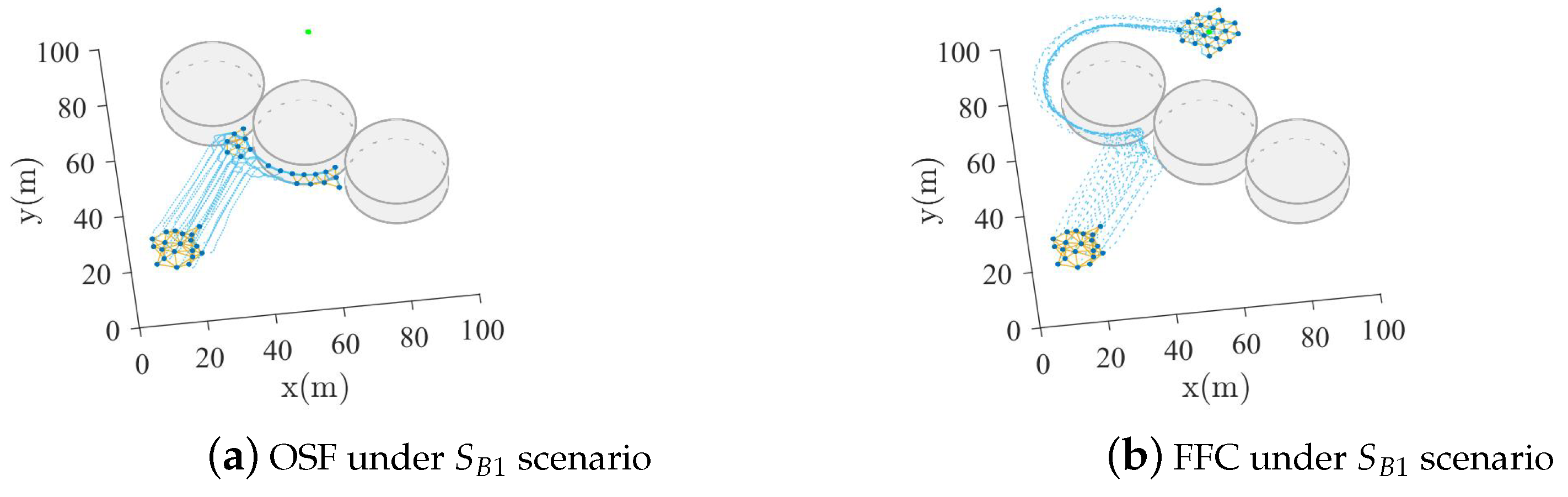
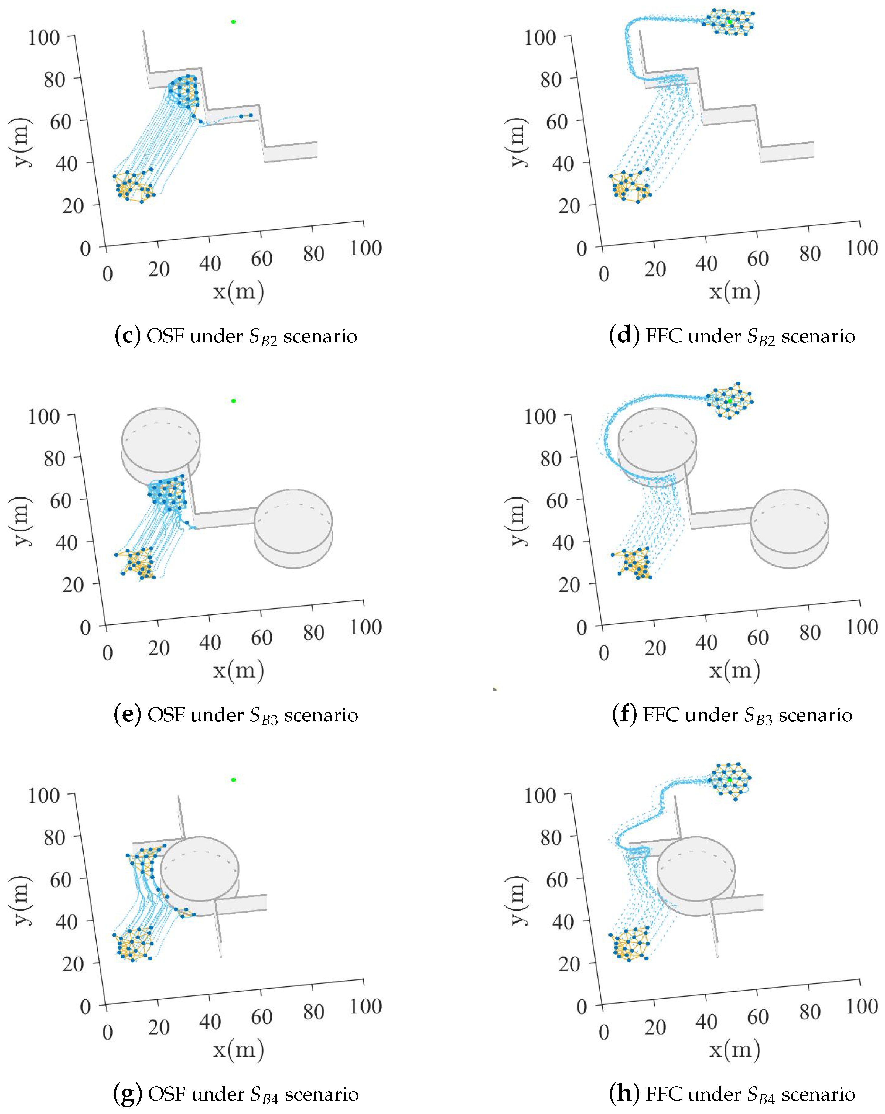
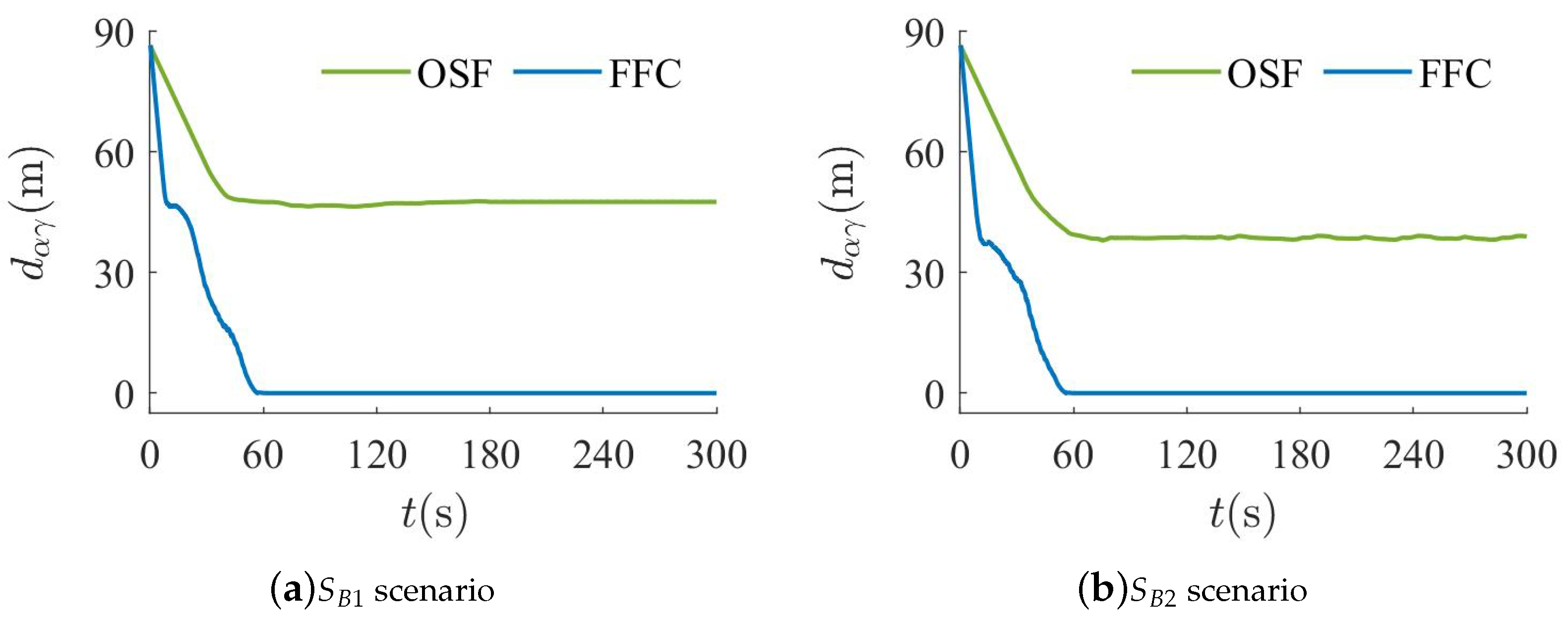
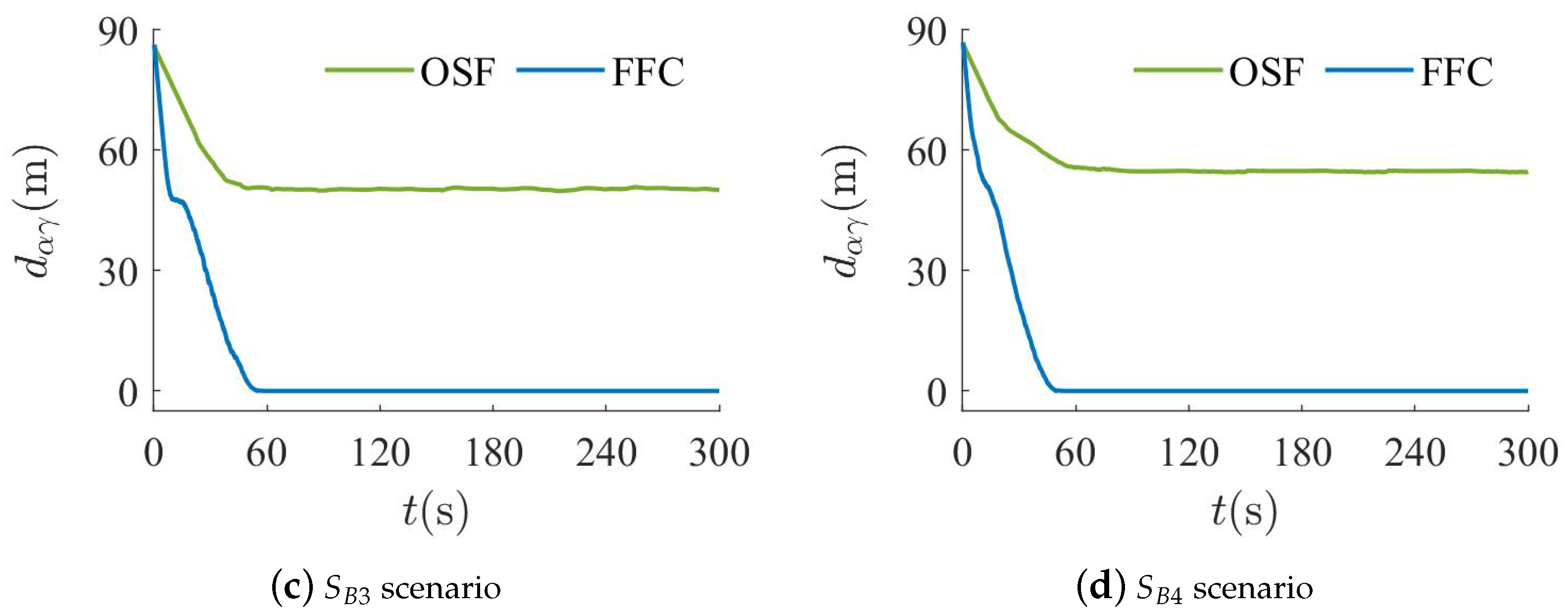
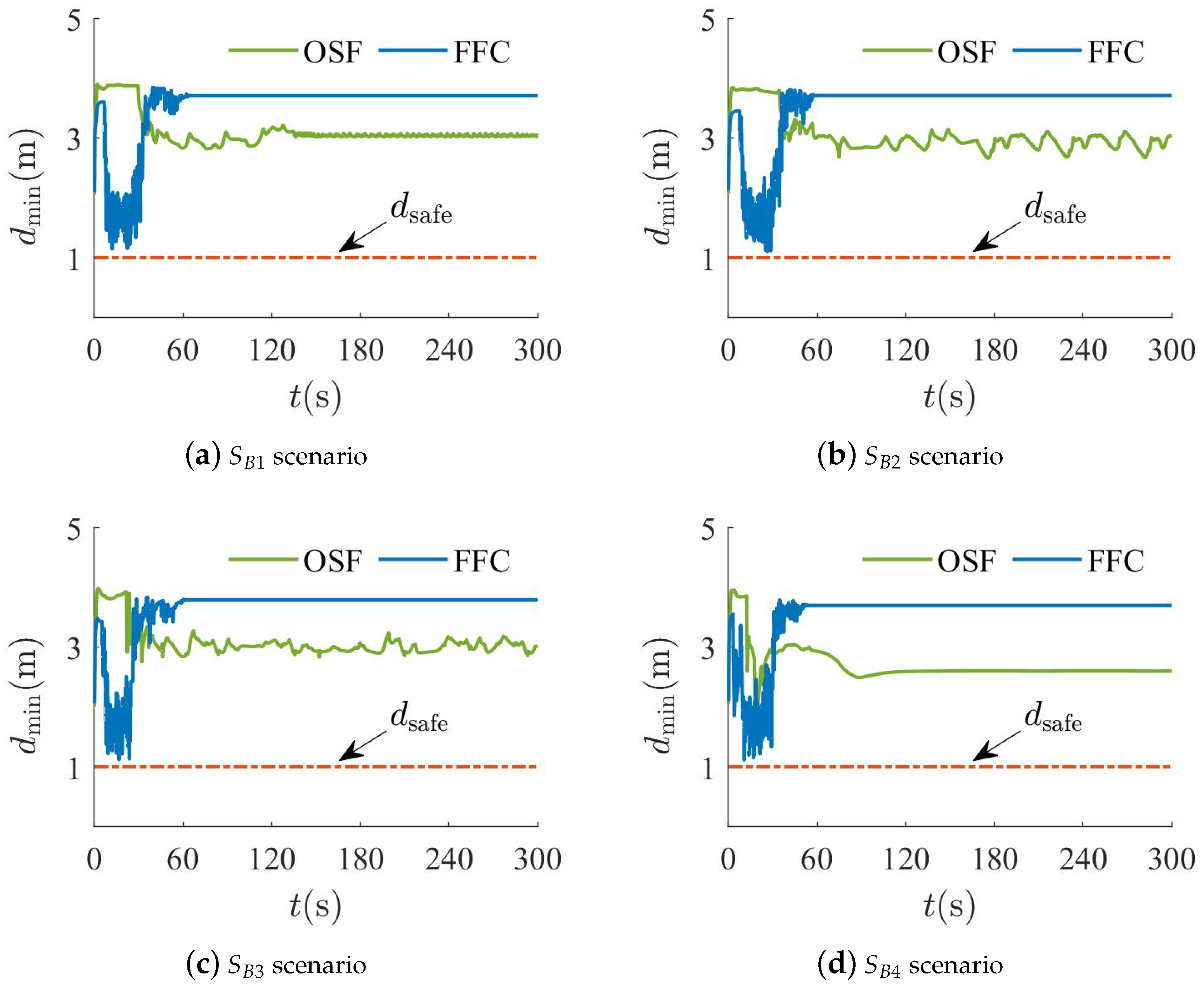
5.2. Spherical and Wall Obstacle Combination Scenario Experiment

In this experiment, four obstacle scenarios are selected as follows:

$S_{B1}$:

There are three spherical obstacles of radius 15 at coordinates $[30, 70]$, $[55, 53]$, and $[80, 36]$.

$S_{B2}$:

There are six wall obstacles of length 20 at coordinates $[25, 85]$, $[25, 65]$, $[45, 65]$, $[45, 45]$, $[65, 45]$, and $[65, 25]$.

$S_{B3}$:

There are two spherical obstacles of radius 15 at coordinates $[30, 70]$ and $[76, 26]$. Moreover, there are two wall obstacles of length 24 at coordinates $[39, 58]$ and $[39, 34]$.

$S_{B4}$:

There is a spherical obstacle of radius 15 at coordinates $[42, 45]$. In addition, there are four wall obstacles of length 20 at coordinates $[38, 80]$, $[18, 60]$, $[46, 30]$, and $[66, 30]$.

The number of $\alpha$-agents is $N=20$, the initial positions of these $\alpha$-agents are selected randomly from ${[5, 20]}^2$, and the initial velocities of these $\alpha$-agents are selected randomly from ${[0, 2]}^2$. In addition, the initial position of the virtual $\gamma$-agent is $[60, 85]$, and the initial velocity of the virtual $\gamma$-agent is zero.

Both visual and quantitative comparisons for the two algorithms are shown in Figure 10, Figure 11 and Figure 12. It can be seen from Figure 10 that almost all $\alpha$-agents of the OSF algorithm remain stationary or oscillate near the combined position of multiple obstacles. Furthermore, it can be observed from Figure 11 that $\alpha$-agents of the OSF algorithm cannot re-aggregate near the $\gamma$-agent. The reason is that $\alpha$-agents are trapped in dynamic equilibrium, and it is difficult to bypass the obstacles. However, the FFC algorithm enables all $\alpha$-agents to bypass the obstacles and follow the $\gamma$-agent. This indicates that the FFC algorithm can enable $\alpha$-agents to escape from the dynamic equilibrium due to the alteration of the virtual force equilibrium. It can be noted from Figure 12 that the minimum distance of the FFC algorithm between the $\alpha$-agent and objects decreases near the combined position of multiple obstacles. Nevertheless, the minimum distance $d_{\min }$ remains greater than the minimum safe distance $d_{\mathrm{safe}}$.

5.3. Complex Obstacle Scenario Experiment

In this experiment, a complex obstacle scenario is selected as follows:

$S_C$:

There are four spherical obstacles of radius 15 at coordinates $[37, 80]$, $[58, 57]$, $[110, 56]$, and $[130, 80]$, and two spherical obstacles of radius 10 at coordinates $[60, 140]$ and $[83, 108]$. Additionally, there are seven wall obstacles of length 10 at coordinates $[25, 40]$, $[45, 30]$, $[65, 20]$, $[85, 10]$, $[135, 5]$, $[135, 145]$, and $[15, 145]$, seven wall obstacles of length 20 at coordinates $[25, 30]$, $[45, 20]$, $[65, 10]$, $[85, 0]$, $[145, 25]$, $[145, 145]$, and $[5, 145]$, two wall obstacles of length $13\sqrt{2}$ at coordinates $[45, 117]$ and $[45, 93]$, and four wall obstacles of length $15\sqrt{2}$ at coordinates $[84, 61]$, $[84, 34]$, $[99, 46]$, and $[69, 46]$.

The number of $\alpha$-agents is $N\in \{10, 20, 40, 70\}$, the initial positions of these $\alpha$-agents are selected randomly from $[6, 30]\times [1, 25]$, and the initial velocities of these $\alpha$-agents are selected randomly from ${[0,2]}^2$. In addition, the initial position of the virtual $\gamma$-agent is $[110, 130]$, and the initial velocity of the virtual $\gamma$-agent is zero.

The visual results of the FFC algorithm in the complex obstacle scenario are shown in Figure 13. It can be seen that all $\alpha$-agents of the FFC algorithm can bypass the complex obstacles and follow the $\gamma$-agent. Furthermore, the quantitative results of the FFC algorithm over 100 runs are shown in Figure 14. It can be observed that as the number of $\alpha$-agents increases, all $\alpha$-agents of the FFC algorithm can still follow the $\gamma$-agent and do not collide with the objects. In summary, the FFC algorithm is suitable for obstacle avoidance in complex obstacle environments.

6. Conclusions

In this paper, we proposed an FFC algorithm to solve the problem of multi-agents trapped in dynamic equilibrium under multiple obstacles. The proposed FFC algorithm calculates the fuzzy expected velocity by the established membership function and fuzzy rules when the agent is trapped in dynamic equilibrium. Furthermore, the FFC algorithm divides the sensing radius region of the agent into four subregions and designs a nonnegative subsection function to adjust the attractive/repulsive potentials in these subregions. The properties analysis demonstrates that multi-agents can achieve collision-free goal-reaching motion when the sufficient conditions in Theorems 1 and 2 are satisfied. The experimental results verify that the proposed algorithm enables multi-agents to escape from dynamic equilibrium and is suitable for obstacle avoidance in complex obstacle environments. However, it is found that the time taken for all agents to bypass obstacles and re-aggregate near the goal position increases with the number of agents. To overcome this problem, we will focus on reducing the computational complexity and improving the scalability of the flocking control algorithm in the future. This includes optimizing the pairwise attractive/repulsive potential and defining multi-agent motion rules. In addition, we will focus on improving the robustness of the flocking control algorithm, such as minimizing sensor noise.

References

1. Yan, C.; Wang, C.; Xiang, X.; Low, K.H.; Wang, X.; Xu, X.; Shen, L. Collision-Avoiding Flocking with Multiple Fixed-Wing UAVs in Obstacle-Cluttered Environments: A Task-Specific Curriculum-Based MADRL Approach. IEEE Trans. Neural Netw. Learn. Syst. 2023, 35, 10894–10908. [Google Scholar] [CrossRef]
2. Tran, V.P.; Garratt, M.A.; Kasmarik, K.; Anavatti, S.G.; Leong, A.S.; Zamani, M. Multi-gas source localization and mapping by flocking robots. Inf. Fusion 2023, 91, 665–680. [Google Scholar] [CrossRef]
3. Shi, L.; Cheng, Y.; Shao, J.; Sheng, H.; Liu, Q. Cucker-Smale flocking over cooperation-competition networks. Automatica 2022, 135, 109988. [Google Scholar] [CrossRef]
4. Li, J.; Zhang, W.; Su, H.; Yang, Y. Flocking of partially-informed multi-agent systems avoiding obstacles with arbitrary shape. Auton. Agents Multi-Agent Syst. 2015, 29, 943–972. [Google Scholar] [CrossRef]
5. Lyu, Y.; Hu, J.; Chen, B.M.; Zhao, C.; Pan, Q. Multivehicle Flocking with Collision Avoidance via Distributed Model Predictive Control. IEEE Trans. Cybern. 2021, 51, 2651–2662. [Google Scholar] [CrossRef] [PubMed]
6. Pignotti, C.; Vallejo, I.R. Flocking estimates for the Cucker–Smale model with time lag and hierarchical leadership. J. Math. Anal. Appl. 2018, 464, 1313–1332. [Google Scholar] [CrossRef]
7. Jiang, W.; Liu, K.; Charalambous, T. Multi-agent consensus with heterogeneous time-varying input and communication delays in digraphs. Automatica 2021, 135, 109950. [Google Scholar] [CrossRef]
8. Zou, Y.; An, Q.; Miao, S.; Chen, S.; Wang, X.; Su, H. Flocking of uncertain nonlinear multi-agent systems via distributed adaptive event-triggered control. Neurocomputing 2021, 465, 503–513. [Google Scholar] [CrossRef]
9. Yu, Z.; Jiang, H.; Hu, C. Second-order consensus for multiagent systems via intermittent sampled data control. IEEE Trans. Syst. Man Cybern. Syst. 2017, 48, 1986–2002. [Google Scholar] [CrossRef]
10. Olfati-Saber, R. Flocking for multi-agent dynamic systems: Algorithms and theory. IEEE Trans. Autom. Control 2006, 51, 401–420. [Google Scholar] [CrossRef]
11. Sakai, D.; Fukushima, H.; Matsuno, F. Flocking for Multirobots Without Distinguishing Robots and Obstacles. IEEE Trans. Control Syst. Technol. 2017, 25, 1019–1027. [Google Scholar] [CrossRef]
12. Jia, Y.; Wang, L. Leader–Follower Flocking of Multiple Robotic Fish. IEEE/ASME Trans. Mechatron. 2015, 20, 1372–1383. [Google Scholar] [CrossRef]
13. Wu, J.; Yu, Y.; Ma, J.; Wu, J.; Han, G.; Shi, J.; Gao, L. Autonomous Cooperative Flocking for Heterogeneous Unmanned Aerial Vehicle Group. IEEE Trans. Veh. Technol. 2021, 70, 12477–12490. [Google Scholar] [CrossRef]
14. Su, H.; Wang, X.; Lin, Z. Flocking of Multi-Agents with a Virtual Leader. IEEE Trans. Autom. Control 2009, 54, 293–307. [Google Scholar] [CrossRef]
15. Zhou, Z.; Ouyang, C.; Hu, L.; Xie, Y.; Chen, Y.; Gan, Z. A framework for dynamical distributed flocking control in dense environments. Expert Syst. Appl. 2024, 241, 122694. [Google Scholar] [CrossRef]
16. Yan, T.; Xu, X.; Li, Z.; Li, E. Flocking of multi-agent systems with unknown nonlinear dynamics and heterogeneous virtual leader. Int. J. Control Autom. Syst. 2021, 19, 2931–2939. [Google Scholar] [CrossRef]
17. Sun, Z.; Xu, B. A flocking algorithm of multi-agent systems to optimize the configuration. In Proceedings of the 2021 China Automation Congress (CAC), Beijing, China, 22–24 October 2021; pp. 7680–7684. [Google Scholar] [CrossRef]
18. Zhao, W.; Chu, H.; Zhang, M.; Sun, T.; Guo, L. Flocking Control of Fixed-Wing UAVs with Cooperative Obstacle Avoidance Capability. IEEE Access 2019, 7, 17798–17808. [Google Scholar] [CrossRef]
19. Qiu, Z.; Zhao, X.; Li, S.; Xie, Y.; Chen, C.; Gui, W. Finite-time formation of multiple agents based on multiple virtual leaders. Int. J. Syst. Sci. 2018, 49, 3448–3458. [Google Scholar] [CrossRef]
20. Duhé, J.F.; Victor, S.; Melchior, P. Contributions on artificial potential field method for effective obstacle avoidance. Fract. Calc. Appl. Anal. 2021, 24, 421–446. [Google Scholar] [CrossRef]
21. Azzabi, A.; Nouri, K. An advanced potential field method proposed for mobile robot path planning. Trans. Inst. Meas. Control 2019, 41, 3132–3144. [Google Scholar] [CrossRef]
22. Semnani, S.H.; Liu, H.; Everett, M.; De Ruiter, A.; How, J.P. Multi-agent motion planning for dense and dynamic environments via deep reinforcement learning. IEEE Rob. Autom. Lett. 2020, 5, 3221–3226. [Google Scholar] [CrossRef]
23. Beaver, L.E.; Malikopoulos, A.A. An overview on optimal flocking. Annu. Rev. Control 2021, 51, 88–99. [Google Scholar] [CrossRef]
24. Szczepanski, R.; Bereit, A.; Tarczewski, T. Efficient local path planning algorithm using artificial potential field supported by augmented reality. Energies 2021, 14, 6642. [Google Scholar] [CrossRef]
25. Song, J.; Hao, C.; Su, J. Path planning for unmanned surface vehicle based on predictive artificial potential field. Int. J. Adv. Rob. Syst. 2020, 17, 1729881420918461. [Google Scholar] [CrossRef]
26. Bayat, F.; Najafinia, S.; Aliyari, M. Mobile robots path planning: Electrostatic potential field approach. Expert Syst. Appl. 2018, 100, 68–78. [Google Scholar] [CrossRef]
27. He, Z.; Chu, X.; Liu, C.; Wu, W. A novel model predictive artificial potential field based ship motion planning method considering COLREGs for complex encounter scenarios. ISA Trans. 2023, 134, 58–73. [Google Scholar] [CrossRef]
28. Szczepanski, R. Safe artificial potential field-novel local path planning algorithm maintaining safe distance from obstacles. IEEE Rob. Autom. Lett. 2023, 8, 4823–4830. [Google Scholar] [CrossRef]
29. Mao, X.; Zhang, H.; Wang, Y. Flocking of quad-rotor UAVs with fuzzy control. ISA Trans. 2018, 74, 185–193. [Google Scholar] [CrossRef] [PubMed]
30. Ntakolia, C.; Moustakidis, S.; Siouras, A. Autonomous path planning with obstacle avoidance for smart assistive systems. Expert Syst. Appl. 2023, 213, 119049. [Google Scholar] [CrossRef]
31. Yu, H.; Zhang, T.; Jian, J. Flocking with obstacle avoidance based on fuzzy logic. In Proceedings of the IEEE ICCA 2010, Xiamen, China, 9–11 June 2010; pp. 1876–1881. [Google Scholar] [CrossRef]
32. Sharma, A.K.; Singh, D.; Singh, V.; Verma, N.K. Aerodynamic Modeling of ATTAS Aircraft Using Mamdani Fuzzy Inference Network. IEEE Trans. Aerosp. Electron. Syst. 2020, 56, 3566–3576. [Google Scholar] [CrossRef]
33. Song, W.; Yang, Y.; Fu, M.; Qiu, F.; Wang, M. Real-Time Obstacles Detection and Status Classification for Collision Warning in a Vehicle Active Safety System. IEEE Trans. Intell. Transp. Syst. 2018, 19, 758–773. [Google Scholar] [CrossRef]
34. Wu, J.; Ji, Y.; Sun, X.; Liang, W. Obstacle Boundary Point and Expected Velocity-Based Flocking of Multiagents with Obstacle Avoidance. Int. J. Intell. Syst. 2023, 2023, 1493299. [Google Scholar] [CrossRef]
Figure 1. The interaction framework between α -agents, γ -agent, and obstacles.
Machines 13 00119 g001
Figure 2. The position and velocity of β -agents in the Olfati-Saber flocking (OSF) algorithm. (a) Infinite wall obstacle. (b) Spherical obstacle.
Machines 13 00119 g002
Figure 3. The scenario of α -agent i being trapped in dynamic equilibrium.
Machines 13 00119 g003
Figure 4. Structure of fuzzy flocking control (FFC) algorithm.
Machines 13 00119 g004
Figure 5. Two membership functions of fuzzy variables.
Machines 13 00119 g005
Figure 6. Four subregions within the sensing radius of α -agent i.
Machines 13 00119 g006
Figure 7. Motion process of the two algorithms in spherical or wall obstacle scenario. The blue dots are the α -agents, the yellow solid line between blue dots is the neighborhood relationship between α -agents, the blue dotted lines are the motion trajectories of α -agents, and the green dot is the γ -agent.
Machines 13 00119 g007
Figure 8. The time taken for all α -agents to bypass obstacles and re-aggregate near the γ -agent over 100 runs in spherical or wall obstacle scenario.
Machines 13 00119 g008
Figure 9. Minimum distance between α -agent and objects over 100 runs in spherical or wall obstacle scenario.
Machines 13 00119 g009
Figure 10. Motion process of the two algorithms in spherical and wall obstacle combination scenario. The blue dots are the α -agents, the yellow solid line between blue dots is the neighborhood relationship between α -agents, the blue dotted lines are the motion trajectories of α -agents, and the green dot is the γ -agent.
Machines 13 00119 g010aMachines 13 00119 g010b
Figure 11. Distance between the center of α -agents and γ -agent in spherical and wall obstacle combination scenario.
Machines 13 00119 g011aMachines 13 00119 g011b
Figure 12. Minimum distance between α -agent and objects in spherical and wall obstacle combination scenario.
Machines 13 00119 g012
Figure 13. Motion process of the FFC algorithm in complex obstacle scenario. The blue dots are the α -agents, the yellow solid line between blue dots is the neighborhood relationship between α -agents, the blue dotted lines are the motion trajectories of α -agents, and the green dot is the γ -agent.
Machines 13 00119 g013
Figure 14. The quantitative results of the FFC algorithm over 100 runs in complex obstacle scenario. (a) The time taken for all α -agents to bypass obstacles and re-aggregate near the γ -agent. (b) Minimum distance between α -agent and objects.
Machines 13 00119 g014