The Secondary Lifting Performance of Crawler Crane Under Delay Coefficient Control Strategy

Abstract

Crawler cranes are mobile lifting equipment used in the process of hoisting goods. After the initial lifting, the crane may need a secondary lift due to adjustments in the position or height of the load. Addressing the common issue of load slipping during the secondary lift caused by hydraulic motor reversal, this study proposes a control strategy applicable to crawler crane secondary lifting. Initially establishing the dynamic characteristics of the secondary lift system, incorporating a delay coefficient, and matching motor pressure build-up with memory pressure, the strategy considers a variable pump input current control to identify the relationship between motor pressure build-up and brake release. Analyzing the dynamic characteristics of secondary lifting under different conditions, this study resolves the issue of hydraulic motor reversal during the second lift caused by heavy loads. The results of this study on crawler crane secondary lifting indicate that, when using a delay coefficient of 0.70 and releasing the brake, no slip phenomenon occurred during the secondary lift process under different load conditions, categorized as 200 tons, 600 tons, and 1000 tons. This ensures the stability and transition quality of the secondary lift, providing theoretical guidance for the control of the crawler crane secondary lifting.

1. Introduction

Crawler cranes play a crucial role in the lifting, transportation, and placement of heavy objects [1,2]. To adjust the position or height of the load, ensure accurate alignment, avoid collisions, or adapt to changes in the working environment, crawler cranes often require a secondary lifting operation. This involves initially lifting the load and then pausing it mid-air to meet specific operational needs. However, secondary lifting is frequently accompanied by load-slipping phenomena [3,4,5,6].

The occurrence of load-slipping phenomena is primarily due to the braking system entering a braking state at the end of the initial lifting phase. When the load is suspended mid-air, the internal leakage within the hydraulic system causes a rapid drop in the pressure of the high-pressure chamber. During the secondary lifting of the load, the braking state of the braking system is released; however, the hydraulic system fails to immediately establish a pressure that balances with the load. As a result, the load may cause the motor to rotate in reverse, leading to undesirable load slipping. This phenomenon can significantly impact the hydraulic system, potentially affecting the normal operation of hydraulic components and shortening their lifespan [7].

Large-tonnage crawler cranes often use electro-hydraulic control technology to ad-dress the issue of secondary lifting [8]. Electrohydraulic control technology employs control algorithms and controllers to manage the primary parameters of the system. Establishing nonlinear matrix equations of the closed-loop control system allows for the study and control of the dynamic characteristics of the lifting system [9,10,11].

In recent years, research on cranes has garnered widespread attention, and various control methods for crawler cranes have demonstrated an excellent performance. The lifting process of cranes involves complex dynamic characteristics, including the tension of the wire rope and the inertia of the hoisted objects [12,13]. Numerous scholars have focused on discussing the dynamic modeling and control methods in crane operations [14,15,16,17]. For instance, Minghui et al. [18] studied the dynamic modeling and anti-sway control methods for slender beam-shaped loads during vertical lifting. Wang et al. [19] proposed a novel anti-sway positioning controller based on a dynamic sliding mode variable structure, suitable for two-dimensional bridge cranes, aiming for precise load positioning. Takahashi H et al. [20] explored the time-optimal control method for suppressing the load sway and arm torsion using a horizontal arm motion in large cranes without sensors. These studies highlight the importance and benefits of dynamic control strategies in crane operations, providing a theoretical foundation and practical guidance for enhancing the safety and efficiency of lifting operations [21,22].

With the rapid development of artificial intelligence, various intelligent algorithms have been widely applied in the field of automatic control, effectively controlling and optimizing the lifting process of cranes. Intelligent algorithms such as a Linear Quadratic Regulator (LQR), fuzzy control, and neural network control have been utilized in crane lifting operations [23,24,25]. For instance, Nming et al. [26] addressed the synchronization control problem in dual-hoist crane systems using neural network control and adaptive robust strategies. Chen et al. [27] conducted in depth research and experimental validation on the active heave compensation system for ship-borne marine cranes using a cascaded NMPC-PID control strategy, providing effective control methods and theoretical support to enhance the safety and efficiency of off-shore lifting operations. Ranjan P et al. [28] highlight innovative methods in energy recovery and position control. These innovations align with the goal of improving the performance and stability of secondary lifting systems by integrating advanced control methodologies and system enhancements.

Previous scholars have made corresponding contributions in theory, simulations, and experiments. But the existing literature provides limited research on the lifting dynamic processes of closed hydraulic systems commonly used in crawler cranes. Moreover, studies on the secondary lifting dynamic characteristics of large crawler cranes’ closed hydraulic systems have not considered the combined simulation of electromechanical and hydraulic integration. This paper addresses the aforementioned issues by establishing the dynamic characteristics of secondary lifting in crawler cranes. A delay coefficient is introduced, and a secondary lifting control strategy suitable for crawler cranes is proposed to resolve the issue of hydraulic motor reversal during the secondary lifting process. Finally, experimental validation confirms that the proposed control method effectively ensures the stability and quality of the transition process during secondary lifting.

This paper is divided into seven sections. Section 1 is the Introduction, Section 2 is the Crane principle, Section 3 is the Electromechanical–Hydraulic Co-Simulation Modeling of the Secondary Hoisting System, Section 4 is the Control Strategy Under the Influence of a Delay Coefficient, Section 5 is the Experimental Study of Secondary Lifting, Section 6 is the Discussion, and Section 7 is the Conclusion.

2. Crane Principle

This chapter introduces the crane principle, which includes the crane working mode, Mathematical Modeling of Secondary Lifting Systems, and analysis of dynamic characteristics of the secondary hoisting system.

2.1. Crane Working Mode

The 1250-ton crawler crane lifting system studied in this paper employs a dual-hoist system, with each hoist driven by two hydraulic pumps and two hydraulic motors. Within each hoist, the two hydraulic motors are mechanically fixed together, sharing nearly identical system parameters. For computational simplicity, the theoretical research in this study focuses solely on one set of closed-loop lifting hydraulic systems, as depicted in Figure 1.

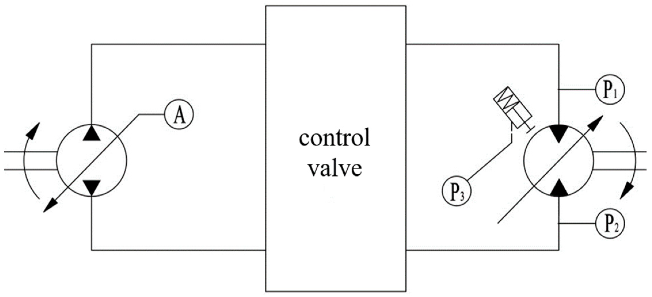
2.2. Mathematical Modeling of Secondary Lifting Systems

The secondary lifting system belongs to the pump-controlled motor system and the dynamic mathematical model of the pump-motor system is derived. Electrical proportional control varies the displacement of the variable pump:

$$D_p=K_p{\gamma }_p$$

(1)

In the equation:

$D_p$—the theoretical displacement of the electrically proportional controlled variable pump (m³/rad);

$K_p$—the gradient of the displacement of the electrically proportional controlled variable pump (m³/rad²);

${\gamma }_p$—the swashplate tilt angle of the electrically proportional controlled variable pump (rad).

The flow equation at the outlet of the electrically proportional controlled variable pump is:

$$q_p=D_p{\omega }_p-C_{ip}(p_h-p_b)-C_{ep}{p}_h$$

(2)

In the equation:

$q_p$—the actual output flow rate of the electrically proportional controlled variable pump (m³/s);

${\omega }_p$—the angular velocity of the electrically proportional controlled variable pump (rad/s);

$C_{ip}$—the internal leakage coefficient of the electrically proportional controlled variable pump ((m³/s)/Pa);

$C_{ep}$—the external leakage coefficient of the electrically proportional controlled variable pump ((m³/s)/Pa);

$p_h$—the high-pressure pressure at the lifting hydraulic system inlet (Pa);

$p_b$—the replenishment pressure in the low-pressure pipeline of the lifting hydraulic system, which typically remains constant and can be treated as such (Pa).

For the calculation of the displacement of the electrically proportional controlled variable motor, the following formula can be used:

$$D_m=K_m{\gamma }_m$$

(3)

In the equation:

$D_m$—the theoretical displacement of the electrically proportional controlled variable motor (m³/rad);

$K_m$—the gradient of the displacement of the electrically proportional controlled variable motor (m³/rad²);

${\gamma }_m$—the swashplate tilt angle of the electrically proportional controlled variable motor (rad).

The continuity equation for the inlet flow of the electrically proportional controlled variable motor is:

$$q_m=C_{im}(p_h-p_{\mathrm{b}})+C_{em}{p}_h+D_m{\displaystyle \frac{\mathrm{d}{\theta }_m}{\mathrm{d}t}}+{\displaystyle \frac{V_0}{{\beta }_e}}{\displaystyle \frac{\mathrm{d}{p}_h}{\mathrm{d}t}}$$

(4)

In the equation:

$q_m$—the actual input flow rate of the electrically proportional controlled variable motor (m³/s).

$C_{im}$—the internal leakage coefficient of the electrically proportional controlled variable motor ((m³/s)/Pa).

$C_{em}$—the external leakage coefficient of the electrically proportional controlled variable motor ((m³/s)/Pa).

${\theta }_m$—the rotational angle of the electrically proportional controlled variable motor (rad).

$V_0$—the total volume of the chamber between the pump outlet and the motor inlet (m³).

${\beta }_e$—the effective bulk modulus (Pa).

Considering $q_p$ = $q_m$, ${\omega }_m={\displaystyle \frac{d{\theta }_m}{dt}}$ as the angular velocity of the electrically proportional controlled variable motor (rad/s) and assuming $p_b$ as a constant and neglecting second-order infinitesimals, the incremental equation is obtained through the Laplace transform:

$$K_p{\omega }_p{\gamma }_p\left(s\right)={K^{\prime }}_m{\gamma }_m\left(s\right)+D_{m0}s{\theta }_m\left(s\right)+\left(C_t+{\displaystyle \frac{V_0}{{\beta }_e}}s\right)P_h\left(s\right)$$

(5)

In the equation:

$C_t$—the total leakage coefficient of the pump and motor, $C_t=C_{tp}+C_{tm}$ ((m³/s)/Pa);

$C_{tp}$—the total leakage coefficient of the electrically proportional controlled variable pump, $C_{tp}=C_{ip}+C_{ep}$ ((m³/s)/Pa);

$C_{tm}$—the total leakage coefficient of the electrically proportional controlled variable motor, $C_{tm}=C_{im}+C_{em}$ ((m³/s)/Pa);

$K_m^{\prime }$—the consumption flow gain, $K_m^{\prime }=K_m{\omega }_{m0}$ (m³/(s·rad));

$D_{m0}$—the initial displacement of the variable motor, $D_{m0}=K_m{\gamma }_{m0}$ (m³/rad);

${\omega }_{m0}$—the initial angular velocity of the motor (rad/s);

${\gamma }_{m0}$—the initial tilting angle of the motor shaft (rad).

In the hydraulic lifting system of a crawler crane, the electric proportional control variable motor is a hydraulic component that counteracts the load. By analyzing the torque balance relationship between the rotating shaft of the hydraulic component and the load, the torque balance equation can be expressed as follows:

$$D_m(p_h-p_b)=J_t{\displaystyle \frac{{\mathrm{d}}^2{\theta }_m}{\mathrm{d}{t}^2}}+B_m{\displaystyle \frac{\mathrm{d}{\theta }_m}{\mathrm{d}t}}+G{\theta }_m+T_L$$

(6)

In the equation:

$J_t$—the total rotational inertia of the variable motor and the load converted on the variable motor shaft (kg·m²);

$B_m$—the viscous-damping coefficient (N·m·s/rad);

G—the torsional spring stiffness of a load (N·m/rad);

$T_L$—all external load torque acting on the variable motor shaft (N·m).

Bringing (3) into (6) and then through the pull transformation, the incremental equation is obtained as follows:

$$K_T{\gamma }_m\left(s\right)+D_{m0}{P}_h\left(s\right)=\left(J_t{s}^2+B_{m}s+G\right){\theta }_m\left(s\right)+T_L\left(s\right)$$

(7)

In the equation:

$K_T$—the motor torque coefficient.

$K_T=K_m{p}_{h0}$ (N·m/rad).

Simultaneously, Equations (5) and (7) eliminate the intermediate variables.

$${\theta }_m={\displaystyle \frac{\frac{D_{m0}{K}_{qp}}{D_m^2}{\gamma }_p+\frac{1}{D_m^2}\left(\frac{V_0{K}_T}{{\beta }_e}s+C_t{K}_T-D_{m0}{K^{\prime }}_m\right){\gamma }_m-\frac{C_t}{D_m^2}\left(1+\frac{V_0}{{\beta }_e{C}_t}s\right)T_L}{\frac{V_0{J}_t}{{\beta }_e{D}_m^2}{s}^3+\left(\frac{C_t{J}_t}{D_m^2}+\frac{B_m{V}_0}{{\beta }_e{D}_m^2}\right)s^2+\left(1+\frac{C_t{B}_m}{D_m^2}+\frac{g{V}_0}{{\beta }_e{D}_m^2}\right)s+\frac{G{C}_t}{D_m^2}}}$$

(8)

From the above, the transfer function block diagram of the electrically proportional control variable pump–electric proportional control variable motor combination of the crawler crane’s lifting hydraulic system is shown in Figure 2.

According to Figure 2, the transfer function can be obtained and the dynamic analysis can be carried out. From the figure, the response relationship between the signal input (${\gamma }_p$ and ${\gamma }_m$), interference input $T_L$, and output ${\theta }_m$ can be seen.

If ${\displaystyle \frac{C_t{B}_m}{D_m^2}}\ll 1$, $G=0$, Equation (8) can be written as:

$${\theta }_m={\displaystyle \frac{\frac{D_{m0}{K}_{qp}}{D_m^2}{\gamma }_p+\frac{1}{D_m^2}\left(\frac{V_0{K}_T}{{\beta }_e}s+C_t{K}_T-D_{m0}{K^{\prime }}_m\right){\gamma }_m-\frac{C_t}{D_m^2}\left(1+\frac{V_0}{{\beta }_e{C}_t}s\right)T_t}{\left(1+\frac{2{\zeta }_h}{{\omega }_h}s+\frac{1}{{\omega }_h^2}{s}^2\right)s}}$$

(9)

In the equation:

${\omega }_h$—the natural frequency of the hydraulic system, ${\omega }_h=\sqrt{{\displaystyle \frac{{\beta }_e{D}_m^2}{V_0{J}_t}}}$ (rad/s);

${\zeta }_h$—the damping ratio of the hydraulic system, ${\zeta }_h={\displaystyle \frac{C_t}{2D_m}}\sqrt{{\displaystyle \frac{{\beta }_e{J}_t}{V_0}}}+{\displaystyle \frac{B_m}{2D_m}}\sqrt{{\displaystyle \frac{V_0}{{\beta }_e{J}_t}}}$.

Therefore, the transfer function of the variable motor angle to the swash plate angle of the variable pump is:

$${\displaystyle \frac{{\theta }_m}{{\gamma }_p}}={\displaystyle \frac{\frac{D_{m0}{K}_{qp}}{D_m^2}}{\left(1+\frac{2{\zeta }_h}{{\omega }_h}s+\frac{1}{{\omega }_h^2}{s}^2\right)s}}$$

(10)

The transfer function of the variable motor angle to the oblique axis angle of the variable motor is:

$${\displaystyle \frac{{\theta }_m}{{\gamma }_m}}={\displaystyle \frac{\frac{1}{D_m^2}\left(\frac{V_0{K}_T}{{\beta }_e}s+C_t{K}_T-D_{m0}{K^{\prime }}_m\right)}{\left(1+\frac{2{\zeta }_h}{{\omega }_h}s+\frac{1}{{\omega }_h^2}{s}^2\right)s}}$$

(11)

The transfer function of the output shaft angle of the variable motor to any accidental load torque is:

$${\displaystyle \frac{{\theta }_m}{T_L}}={\displaystyle \frac{-\frac{C_t}{D_m^2}\left(1+\frac{V_0}{{\beta }_e{C}_t}s\right)}{\left(1+\frac{2{\zeta }_h}{{\omega }_h}s+\frac{1}{{\omega }_h^2}{s}^2\right)s}}$$

(12)

2.3. Analysis of Dynamic Characteristics of the Secondary Hoisting System

Through the analysis of the mathematical model of the closed hydraulic system of the crawler crane, because the displacement gradient of the pump and the total leakage coefficient of the pump-controlled hydraulic motor are constant, the speed gain ${\displaystyle \frac{K_{qp}}{D_m}}$ and static speed flexibility ${\displaystyle \frac{C_t}{D_m^2}}$ of the pump-controlled hydraulic motor are relatively constant. It can be found that the dynamic characteristics of the secondary lifting are related to the displacement and load of the variable pump.

The larger the lifting load is, the more hydraulic oil is needed for pressure building, and the large displacement of the variable pump will affect the dynamic characteristics of the secondary lifting. The displacement should not be too small, as it will lead to a slow pressure build and even lead to the establishment of pressure that cannot overcome the load.

3. Electromechanical–Hydraulic Co-Simulation Modeling of Secondary Hoisting System

This chapter introduces the electromechanical–hydraulic co-simulation modeling of the secondary hoisting system, which includes the simulation model establishment, simulation model boundary condition setting, and simulation without a control strategy.

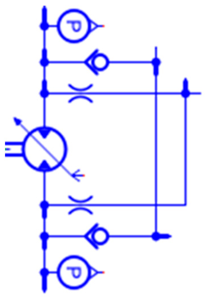
3.1. Simulation Model Establishment

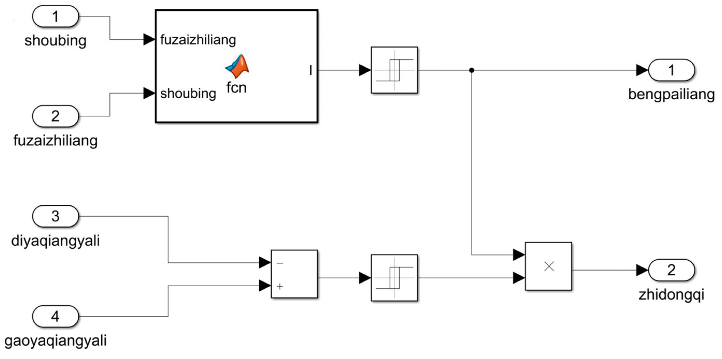
3.1.1. Simulation Modeling of the Electric Control System of Lifting Mechanism

The electric control system calculates the displacement current of the electric proportional control variable pump according to the load mass and the handle signal, and then judges whether the pressure difference between the two ends of the motor reaches the set value according to the delay coefficient to control the opening and closing of the brake. The control strategy block diagram of the secondary lifting action is shown in Figure 3.

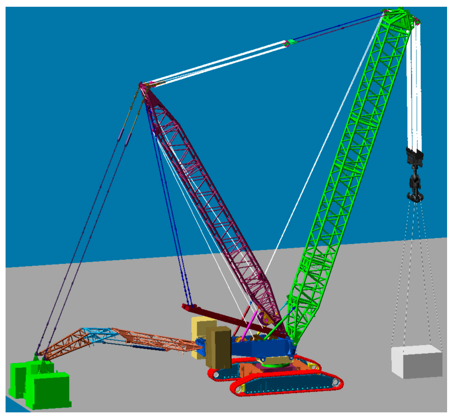
3.1.2. Mechanical Dynamics Simulation Modeling of Lifting Mechanism

In this section, the kinematics simulation is used to model and simulate the lifting mechanism of the crawler crane, which can feedback the force of the hydraulic system in the joint simulation model, and can also reproduce the secondary lifting movement process of the crawler crane.

Since the actual structure of the crawler crane is complex and the number of parts is large, the detailed establishment of the model has a high cost of simulation calculation, so the model needs to be simplified. As this topic only studies the lifting mechanism, the mechanical system model can be simplified as the crawler walking part, the rotary platform part, the main arm, the super-lifting mast, the main mast, the counterweight, the wire rope, the fixed pulley, the moving pulley, the winch, the hook, and so on. According to the actual parameters of the mechanical part of the 1250 t crawler crane, a three-dimensional simulation model is established, as shown in Figure 4.

After the three-dimensional model is established, the constraints and drives of each part are added. Constraints mainly include revolute pairs, moving pairs, and fixed constraints. The main volume 1 and the main volume 2 of the crawler crane are added with the drive, respectively. After the drive is added, it is necessary to verify whether the working device has a certain movement by calculating the degree of freedom and simulating the operation.

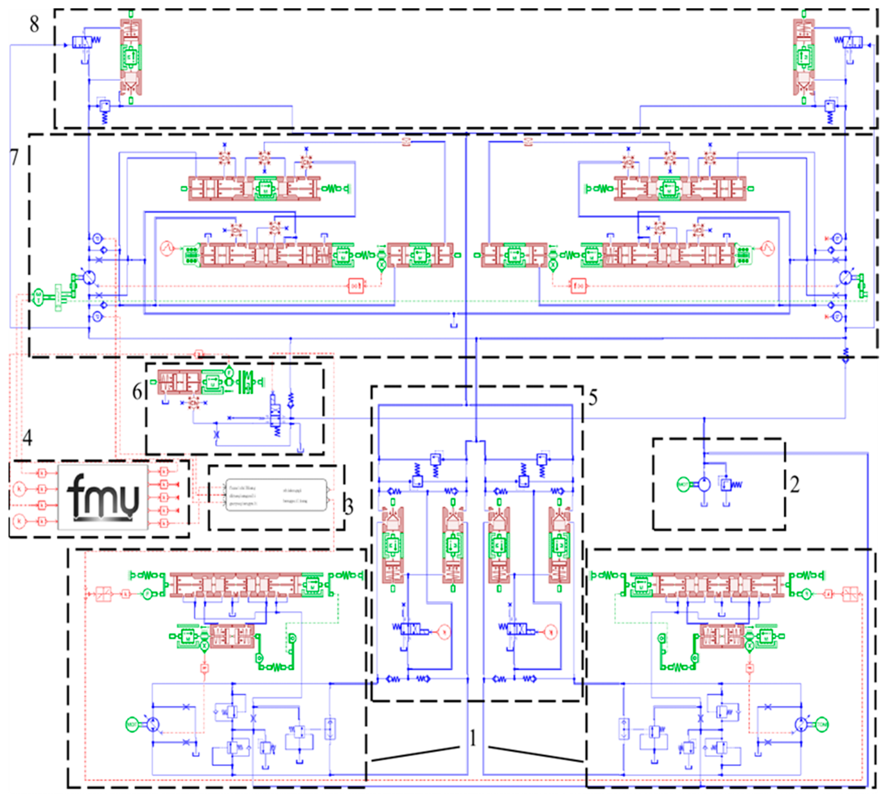
3.1.3. Joint Simulation Model Establishment

The hydraulic system, electric control system, and mechanical system of the 1250 t crawler crane are integrated, and the final simulation model is shown in Figure 5.

3.2. Simulation Model Boundary Condition Setting

Table 1. Main parameters of the hoisting system simulation model.

System Parameter	Numerical Value
Engine parameter (r/min)	1200
Hydraulic oil density (kg/m3)	850
Viscosity of hydraulic oil (mm2/s)	46
The maximum displacement of the main pump (mL/r)	125
Maximum displacement of motor (mL/r)	160
Replenishment pump displacement (mL/r)	52
Compensating oil pressure (bar)	30
Maximum system pressure (bar)	350
Brake-opening pressure (bar)	20
Diameter of drum (m)	0.7
Speed ratio	99
Part line of pulley block	62
Diameter of wire rope (mm)	32
Payload mass (t)	200–1200

presents the main parameters of the hoisting system simulation model. detailing the critical variables that define the system’s behavior.

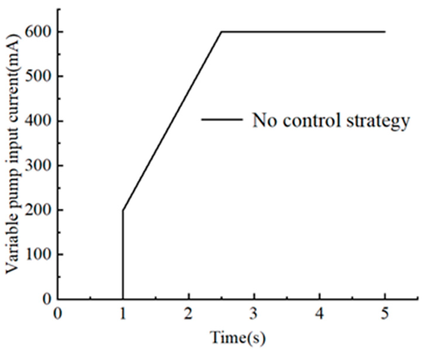
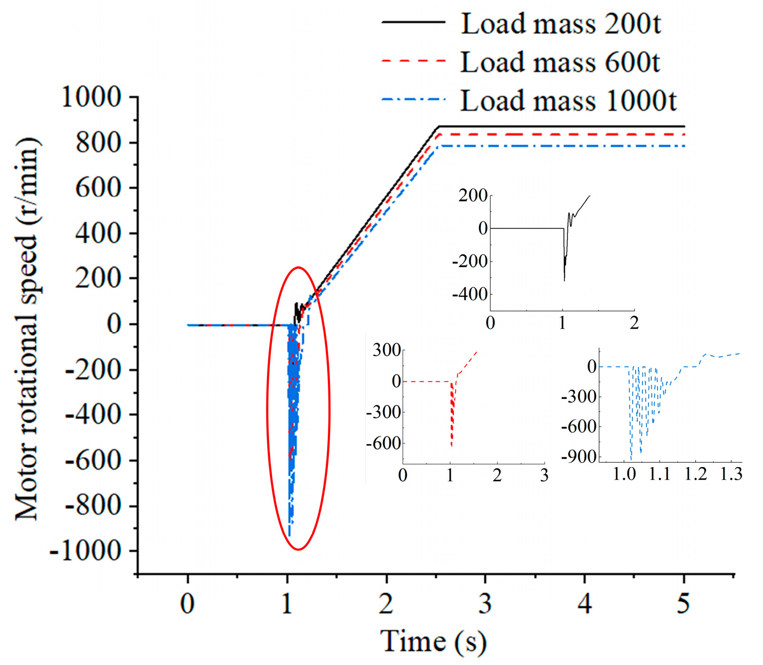
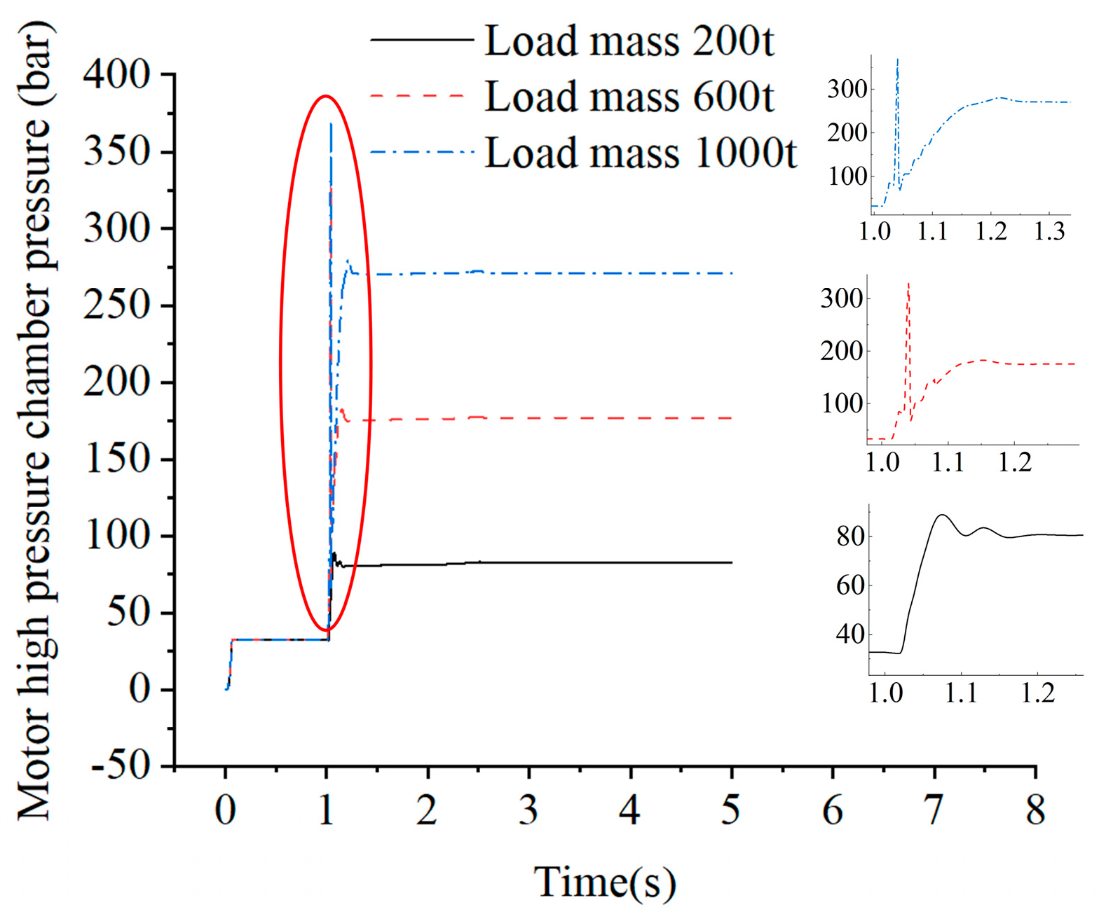
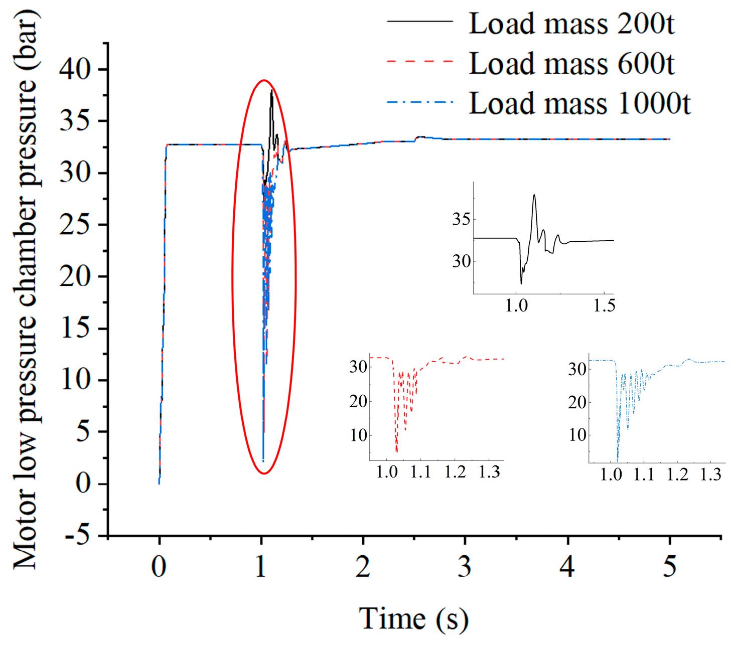
3.3. Simulation Without Control Strategy

The model is controlled by the handle control variable pump to control the system action. When the handle slope rise signal is given at 1 s, it usually takes 1–2 s for the handle to reach the maximum value from the middle. In this study, 1.5 s is taken for the joint simulation analysis of the lifting action. The input current model number of the variable pump is shown in Figure 6.

In this simulation study, the secondary lifting control strategy is not added, that is, the electromagnetic valve of the brake is powered at the same time as the lifting handle acts, which can reproduce the phenomenon of secondary lifting and sliding and verify the accuracy of the model in subsequent experimental studies.

The maximum lifting capacity of the crawler crane studied in this paper is 1250 t. The load mass is selected as 200 t, 600 t, and 1000 t in the range of the lifting capacity. The simulation time is 3 s and the sampling interval is 0.001 s. The obtained motor speed and pressure curves at both ends of the motor are shown in Figure 7, Figure 8 and Figure 9.

From Figure 7, Figure 8 and Figure 9, it can be seen that in the absence of a control strategy, the motor reversal phenomenon occurs when the loads of different masses are lifted twice, and the increase in the load mass leads to the greater motor reversal speed. The reversal speed of the motor is close to 1000 r/min under the condition of a 1000 t load. Due to the reversal of the motor, the pressure of the low-pressure chamber decreases to varying degrees, and even reaches 0 bar at 1000 t. From the high-pressure chamber curve of the motor, it can be seen that there is a pressure shock phenomenon in both the 600 t load and 1000 t load. This is because the pressure drop in the low-pressure chamber triggers the explosion-proof valve, and the explosion-proof valve is quickly closed. The closed pipeline of the high-pressure chamber of the motor is greatly reduced. The sliding of the heavy object has an instantaneous impact on the high-pressure chamber of the motor, and the pressure of the high-pressure chamber of the motor increases sharply to more than 350 bar. Due to the small mass of the 200 t weight, the reversal speed is not enough to reduce the pressure of the low-pressure chamber of the motor to trigger the explosion-proof valve. Therefore, there is no pressure mutation in the high-pressure chamber of the motor.

4. Control Strategy Under the Influence of Delay Coefficient

This chapter introduces the control strategy under the influence of the delay coefficient, which includes the control strategy design and the simulation of the control strategy.

4.1. Control Strategy Design

To avoid the phenomenon of secondary lifting and sliding, the control strategy of the delayed opening of the brake is adopted. In this paper, the pressure memory control algorithm is used for the solenoid valve of the normally closed brake. The pressure memory control algorithm refers to the process of the secondary lifting of the load. The controller uses the pressure difference between the two sides of the motor at the last instance of the lifting stability of the system as the memory pressure to realize the control of the secondary lifting of the load. When the load is lifted twice, the control system detects the pressure at both ends of the system motor to calculate the pressure difference. Compared with the memory pressure, when the pressure difference at both ends of the motor reaches the memory pressure, the controller outputs the signal to the brake the solenoid valve to control the brake solenoid valve and make it open; therefore, the braking state is lifted accordingly. The premature opening and late opening of the brake will adversely affect the hydraulic system. Therefore, it is very important to use the controller to control the opening time of the brake for the dynamic characteristics of secondary lifting.

As shown in Figure 10, when t = 0, the secondary lifting process begins. t1 is the delay time of the solenoid valve of the normally closed hydraulic brake and t2 is the time re-quired for the opening of the solenoid valve of the normally closed hydraulic brake. Tstart is the torque of the hydraulic motor that is exactly equal to the braking torque of the normally closed hydraulic brake, and the hydraulic motor can rotate at this time. t3 is the time when the normally closed hydraulic brake is fully opened. The control strategy of the anti-secondary lifting and sliding of the crawler crane is mainly to adjust the time t1 of the electromagnetic valve delay. Since the opening of the normally closed hydraulic brake requires a certain time, it is not an instant open, so the time point when the hydraulic motor starts to rotate will not exceed the fully open time of the normally closed hydraulic brake. The opening process of the normally closed hydraulic brake has a great influence on the closed hydraulic system, and the fully open time t3 of the normally closed hydraulic brake directly affects the setting of the delay time t1 of the solenoid valve, which will affect the dynamic characteristics of the secondary lifting process of the crawler crane.

As shown in Figure 11, to realize the pressure memory function, a pressure control system is added at both ends of the motor. The pressure sensor is installed on the high-pressure side and the low-pressure side of the motor, and the opening of the solenoid valve of the braking system is controlled by setting the memory pressure.

The opening time of the brake is determined by adjusting the delay coefficient. In this paper, the delay coefficient is defined as the ratio of the pressure difference at both ends of the motor to the memory pressure, that is:

$$K_d={\displaystyle \frac{\Delta p_m}{p_j}}$$

(13)

In the equation:

$\mathsf{\Delta }{p}_m$—the real-time differential pressure at both ends of the motor, $\Delta p_m=p_{mh}-p_{ml}$ (bar);

$p_j$—the memory pressure, that is, the pressure difference (bar) at both ends of the hydraulic motor during the normal operation of the lifting system;

$p_{mh}$—the current real-time measured high-pressure-side pressure value (bar) of the hydraulic motor;

$p_{ml}$—the current real-time measured low-pressure-side pressure value of the hydraulic motor (bar).

Assuming that when the controller sends a signal, the process of the brake is fully opened instantly, then the pressure difference between the two ends of the motor is equal to the memory pressure opening, and the secondary lifting and sliding phenomenon will not occur. At this time, the delay coefficient $K_d$ is equal to 1. However, in reality, the brake is not opened instantaneously, so the delay coefficient $K_d$ should be less than 1. In the process of the delayed opening of the brake, the pressure difference between the two ends of the motor reaches the memory pressure to avoid the secondary lifting weight falling and will not cause too much of a pressure impact.

The secondary lifting action of the crane is to increase the pump displacement by pushing the variable pump power proportional handle; then, when the pressure difference between the two ends of the motor reaches a certain value, the brake solenoid valve is opened to open the brake. The dynamic performance of secondary lifting under different displacements is different, so the influence of the variable pump operation mode on the dynamic characteristics of secondary lifting is different. In this paper, considering that the pressure difference of different loads in secondary lifting is large, if the displacement of the variable pump is uniform, the opening time difference is also large. To minimize the difference in the opening time under the same control strategy, this paper will use different variable pump displacements for different loads. In fact, without considering the leakage, the pressure change in the pipeline is proportional to the input flow, the input flow is proportional to the displacement of the variable pump, and the pressure required to overcome the load is proportional to the load mass. Therefore, the variable pump input current control strategy used at different loads is as follows:

$$K_I=k_{0}m$$

(14)

In the equation:

$K_I$—the electrical proportional control variable pump current gradient (mA/s);

$k_0$—the proportionality factor;

$m$—the load mass (t).

The maximum lifting weight of the crane studied in this paper is 1250 t. The research on the dynamic performance of secondary lifting selects 200 t, 600 t, and 1000 t as the research object, without considering other disturbances such as the wind load. When the load is different, the pressure required by the system and the opening pressure of the brake are different. At this time, whether the dynamic characteristics of the system are the same, these problems will be the focus of this section. In order to facilitate the simulation of the secondary lifting dynamic process, this paper gives three linear input methods for different lifting weights, and the displacement current gradient current increases linearly with the increase in the weight.

The control strategy under the delay co-efficient: the proportional coefficient is set to 0.1, and the pump displacement current gradients corresponding to 200 t, 600 t, and 1200 t weights are 20 mA/s, 60 mA/s, and 100 mA/s, respectively.

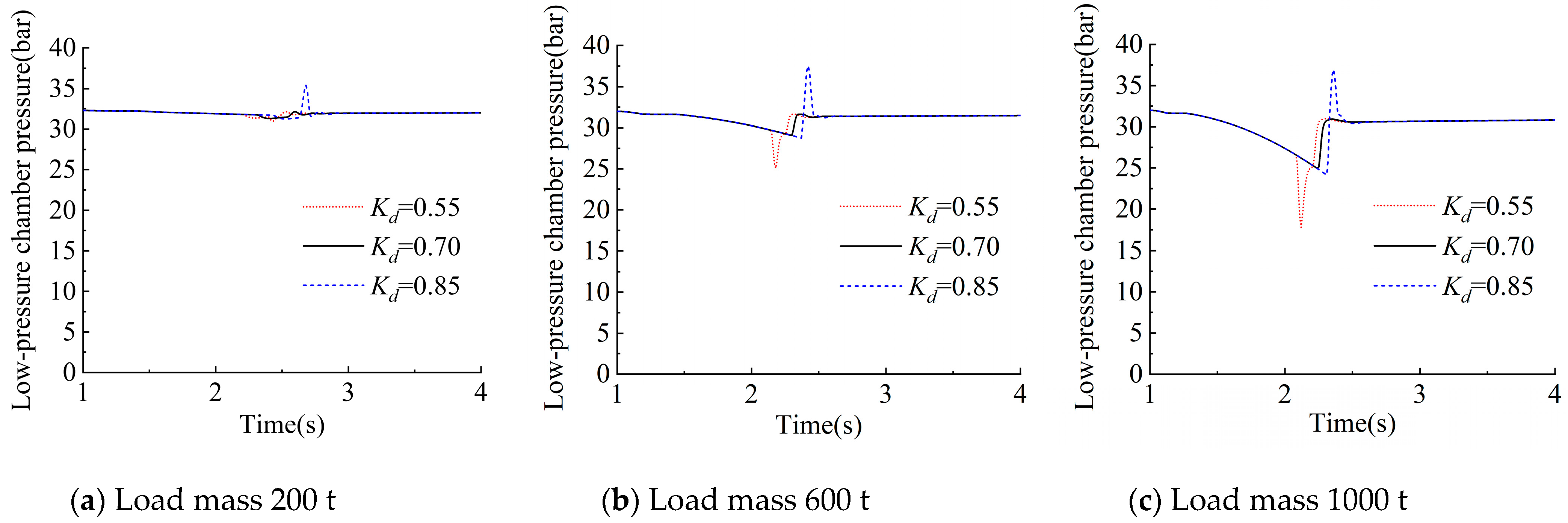
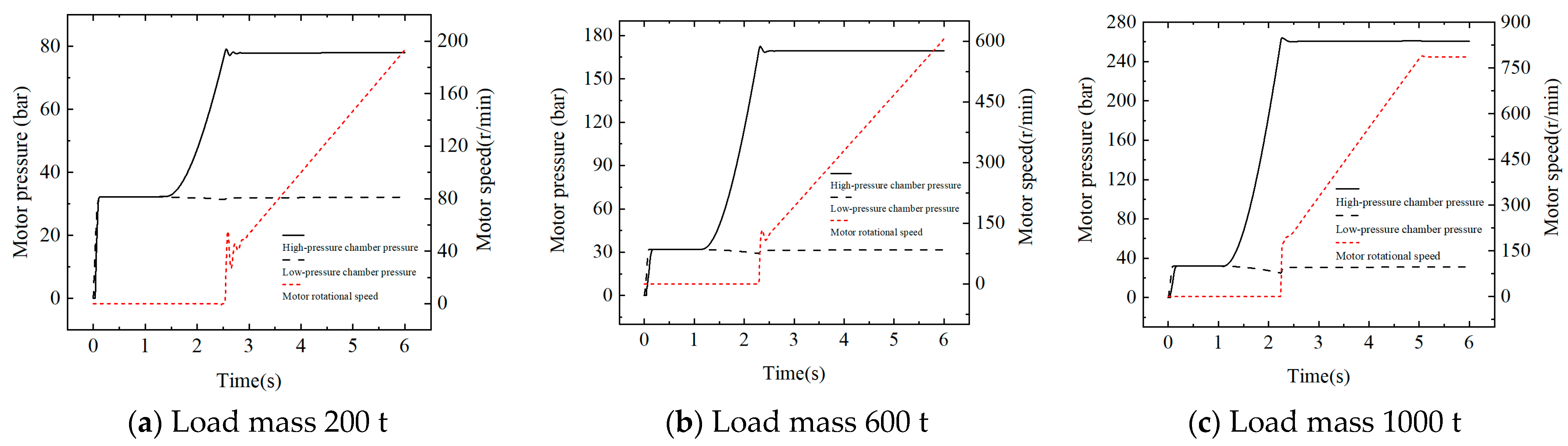
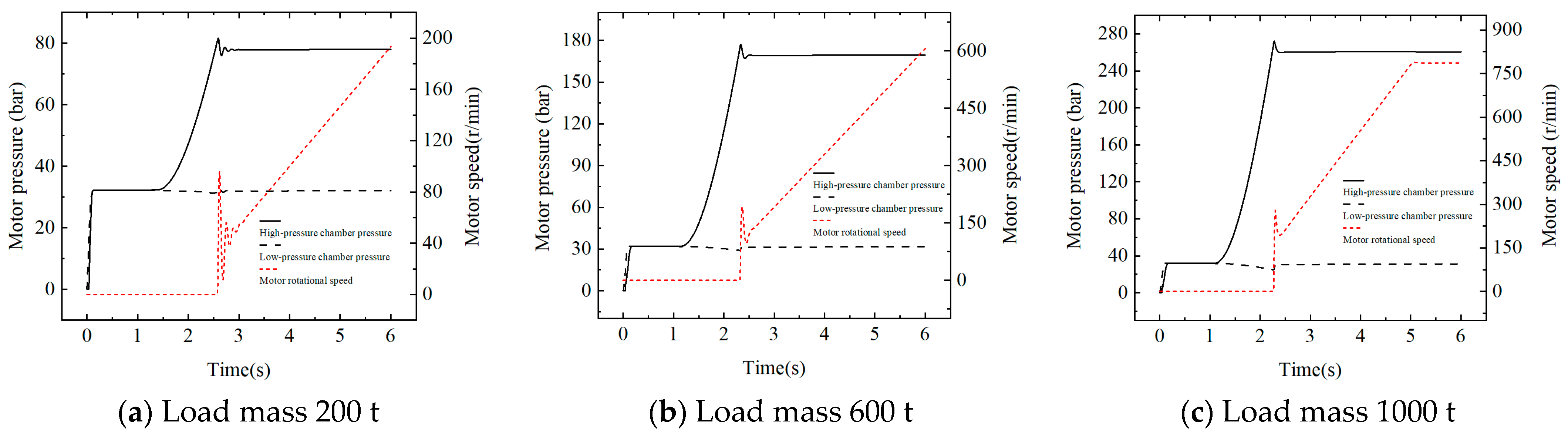
4.2. Simulation of Control Strategy

Generally, the research on the dynamic characteristics of the lifting hydraulic system mainly includes two aspects: stability and excessive process quality. The optimization goal of the secondary lifting dynamic performance of the lifting system is to ensure that the system pressure overshoot is less than 5% under the premise of ensuring that the phenomenon of secondary lifting and sliding does not appear in the system, and the motor delay start time cannot be too long.

(1)

A simulation study on the influence of the dynamic performance of secondary lifting.

Different delay coefficients $K_d$ are set for the control strategy, the setting range is [0.55, 0.85], the secondary lifting action starts from 1 s, and the simulation step size is 0.001 s. The pressure results of the high-pressure cavity of the motor obtained by the joint simulation are shown in Figure 12.

The lifting system uses the control strategy for secondary lifting and the simulation results of the motor speed are shown in Figure 13.

The lifting system uses the control strategy for secondary lifting and the simulation results of the low-pressure chamber pressure of the motor are shown in Figure 14.

Through the previous simulation analysis, it can be seen that the dynamic characteristics of the system are quite different when the control strategy has different delay coefficients. The secondary lifting performance parameters under the control strategy are shown in

Table 2. Secondary lifting performance parameter table under control strategy.

Load Mass (t)	Retardation Coefficient Kd	Motor Reverse Speed (r/min)	Pressure Overshoot of High-Pressure Chamber	Low-Pressure Chamber Minimum Pressure (bar)	Motor Delay Time (s)
200	0.55	58.9	1.7%	31	1.47
200	0.70	0	1.6%	31.4	1.54
200	0.85	0	8.8%	31.3	1.63
600	0.55	163.3	2.2%	25.1	1.25
600	0.70	0	2%	29	1.3
600	0.85	0	1.8%	28.8	1.37
1000	0.55	248.1	1.8%	17.8	1.2
1000	0.70	0	1.5%	24.8	1.25
1000	0.85	0	9.1%	24.1	1.31

.

From the data in Figure 12, Figure 13 and Figure 14 and Table 2, it can be seen that when the delay coefficient is set to 0.55, the hydraulic motor reverses when the crane performs secondary lifting with different mass loads, that is, the secondary lifting and sliding phenomenon occurs, and the motor reverses with the increase in the load mass, increasing the speed. This is because the system pressure does not reach the memory pressure brake which has been fully opened, resulting in a load decline phenomenon. It is not appropriate to carry out secondary lifting when the delay coefficient is 0.55.

When the delay coefficient is 0.85, there is no secondary lifting and sliding phenome-non in the secondary lifting of the crane with different mass loads. However, due to the long delay time, the pressure of the high-pressure chamber of the motor is too high, and the pressure overshoot is more than 8%, resulting in a large fluctuation of the motor speed, which seriously affects the performance of the secondary lifting. It is not appropriate to carry out secondary lifting when the delay coefficient is 0.85.

When the delay coefficient is 0.70, there is no secondary lifting and sliding phenome-non in the secondary lifting of the crane with different mass loads, the fluctuation of the system pressure and the motor speed is small, and the system stability and the quality of the transition process are good, which shows that it is reasonable to carry out secondary lifting when the delay coefficient is 0.70.

The simulation results show that when using the control strategy, the controller sets the delay coefficient to 0.70, and the secondary lifting performance of the crane meets the optimization target requirements. In addition, it can be found from Table 2 that when the delay coefficient is set to 0.70 in the control strategy, the average start-up time of the motor is 1.36 s, and the average overshoot of the high-pressure chamber pressure of the motor is 1.7%.

(2)

Simulation research on secondary lifting control strategy after adding interference.

Through simulation analysis, it is found that the crawler crane can effectively improve the secondary lifting performance after adding the control strategy. However, there are various interference factors in the lifting system during actual secondary lifting, which may lead to an unstable brake-opening time. Therefore, it is necessary to analyze the anti-interference ability of the control strategy. In this paper, the research method of the anti-interference ability is to modify the opening time of the brake, and the anti-interference ability of the control strategy is analyzed by the controller in two cases of 70 ms ahead and a 70 ms delay of the brake control valve based on the original opening time.

Under the control strategy of selecting the optimal delay coefficient, the actuator activation time is advanced by 70 ms. Using combined simulation methods, the simulation results, as shown in Figure 15, include three main components: the high-pressure chamber pressure of the hydraulic motor, the low-pressure chamber pressure of the hydraulic motor, and the rotational speed of the hydraulic motor.

Under the control strategy of selecting the optimal delay coefficient, the actuator activation time is delayed by 70 ms. Using combined simulation methods, the simulation results, as shown in Figure 16, include three main components: the high-pressure chamber pressure of the hydraulic motor, the low-pressure chamber pressure of the hydraulic motor, and the rotational speed of the hydraulic motor.

The secondary lifting performance parameters of the control strategy with interference are shown in

Table 3. Secondary lifting performance parameter table with the interference control strategy.

Load Mass (t)	Brake Interference Opening Time (ms)	Motor Reverse Speed (r/min)	Pressure Overshoot of High-Pressure Chamber
200	−70	0	1.6%
600	−70	0	2%
1000	−70	0	1.5%
200	+70	0	4.8%
600	+70	0	4.7%
1000	+70	0	4.5%

.

From the simulation results shown in Figure 15 and Figure 16 and Table 3, it can be seen that under the control strategy of different loads of 200 t, 600 t, and 1000 t, the brake does not slide down 70 ms in advance, and the fluctuation of the speed and pressure is small. The average value of the pressure overshoot in the high-pressure chamber is 1.7%, which meets the requirements of the optimization goal. Under the control strategy, there is no sliding phenomenon when the brake is delayed by 70 ms, and the speed and pressure fluctuations are also small. The average pressure overshoot of the high-pressure chamber is 4.67%, which also meets the requirements of the optimization target.

In summary, the stability of the system and the quality of the transition process still meet the optimization goal of the dynamic performance of the secondary lifting of the lifting system when the control strategy with interference is added, and it has the certain anti-interference ability.

5. Experimental Study of Secondary Lifting

5.1. Experimental Scheme

To reduce the number of experimental errors and increase the credibility of the experiment, each action in this experiment needs to be repeated four times in a row, and the four pieces of experimental data are analyzed and compared. Multiple experiments can effectively avoid the contingency of a single experiment and ensure the authenticity and rationality of the experimental data. The secondary lifting experiment adopts a 1250 t crawler crane, and the experimental field is the company’s special debugging field, as shown in Figure 17.

The field photos of the sensor installation wiring and electrical control system of the 1250 t crawler crane are shown in Figure 18, Figure 19, Figure 20 and Figure 21.

In the secondary lifting experiment, the engine speed is set to 1200 r/min. Firstly, the 1000 t load without a control strategy is tested to verify the accuracy of the simulation model. Then, the secondary lifting control strategy is added to the controller, and the secondary lifting experiments of the 200 t and 600 t loads are carried out to verify the rationality of the control strategy. To ensure the validity and accuracy of the experimental data, each group of actions is repeated 4 times, and a set of normal experimental data is taken for secondary lifting performance analysis. The experimental scheme is shown in

Table 4. Secondary lifting experimental scheme of 1250 t crawler crane.

	Control Strategy	Load Mass	Initial State	Handle Action
1	no	1000 t	The weight is 0.5 m off the ground.	The weight-lifting handle is slowly pushed to the bottom; keep; the handle slowly returns to the median
2	yes	200 t
3	yes	600 t

.

5.2. Experimental Test Results and Analysis of No Control Strategy

According to the experimental principle and the experimental scheme of the secondary lifting action, the posture of the crane is adjusted to maintain stability. The load is 1000 t, the initial state is 0.5 m from the ground, and the weight-lifting handle takes 1.5 s to slowly push to the bottom. After some time, the handle slowly returns to the middle. The experiment is repeated, the collected experimental data are extracted and sorted, and a better set of experimental results are obtained, as shown in Figure 22.

By comparing the simulation curve and experimental curve of the input current signal of the electric proportional control variable pump without a control strategy in Figure 22a, it can be seen that the change trend and specific value of the displacement current signal of the variable pump are the same during the experimental test. Due to the signal interference, sensor accuracy, and controller output efficiency, the displacement signal of the variable pump in the experimental test is not a smooth curve, but a step-up and is unstable.

By comparing the simulation curve and experimental curve of the high-pressure chamber pressure of the motor without a control strategy in Figure 22b, it can be seen that the secondary lifting action begins at 1 s. From Figure 22d, it can be seen that because there is no control strategy brake, the hydraulic motor starts to reverse by the heavy object, and the high-pressure chamber pressure of the hydraulic motor rises rapidly and steadily. When the experimental test is at 1.05 s, the pressure of the high-pressure chamber is 98 bar. At this time, the instantaneous impact of the pressure occurs in the high-pressure chamber of the hydraulic motor. The impact pressure reaches 400 bar and returns to normal at 1.07 s. The impact time lasts about 20 ms. When the simulation is at 1.03 s, the pressure of the high-pressure chamber is 84 bar and the pressure’s instantaneous impact occurs in the high-pressure chamber of the hydraulic motor. The impact pressure reaches 370 bar, returns to normal at 1.04 s, and the impact time lasts about 10 ms. Both the experimental test and the simulation show the phenomenon of instantaneous pressure impact. The impact time difference is 10 ms and the maximum impact pressure difference is 7.5%. The simulation data are consistent with the experimental test.

The experimental test shows that the high-pressure cavity of the hydraulic motor reaches the maximum pressure at 1.4 s, but the pressure of the high-pressure cavity of the hydraulic motor is in a fluctuating state. This is mainly because the lifting speed is too fast, and the large load mass causes the mechanical structure such as the boom to vibrate, which leads to a certain degree of fluctuation in the pressure of the hydraulic system. The average value of the high-pressure cavity of the experimental motor after a steady state is 273 bar by data processing software. When the simulation is at 1.3 s, the high-pressure cavity of the hydraulic motor reaches the maximum pressure. Since the simulation model treats the mechanical structure as a rigid part, the pressure of the high-pressure cavity is stable at 270 bar. The steady-state pressure difference between the experimental test and simulation is small and the simulation accuracy is good.

By comparing the simulation curve and the experimental curve of the low-pressure chamber pressure of the motor without a control strategy in Figure 22c, it can be seen that the pressure of the low-pressure chamber of the motor decreases rapidly after the start of secondary lifting. This is because the motor reverses too fast and the oil flow is not enough when there is no control strategy. When the experimental test is at 1.01 s, the pressure of the motor drops sharply. The pressure at the low-pressure port of the motor drops from 31 bar to about 2 bar. After a period of oscillation, the pressure returns to normal at 1.2 s, but there is a large fluctuation. This is mainly because the lifting speed is too fast and the large load mass makes the mechanical structure such as the boom vibrate, resulting in a certain degree of fluctuation in the pressure of the hydraulic system.

Comparing the simulation curve and experimental curve of the brake port pressure of the motor without a control strategy in Figure 22d, the pressure fluctuation phenome-non similar to the low-pressure chamber of the motor appears after secondary lifting, which is mainly caused by the insufficient oil flow. Compared with the experimental data, it can be seen that the simulation also showed a sudden drop in the pressure of the low-pressure chamber of the motor at 1.01 s. The pressure of the low-pressure chamber of the motor decreased from 32.5 bar to about 2.5 bar. After a period of vibration, the pressure returned to normal at 1.25 s. The simulation was consistent with the experiment.

Based on the above comparison between the simulation and experimental test without a control strategy, it can be found that the fitting degree between the simulation and experimental test is good. The electromechanical–hydraulic co-simulation can reproduce secondary lifting and the sliding phenomenon in the experimental test, which proves that the simulation established in this paper has good accuracy.

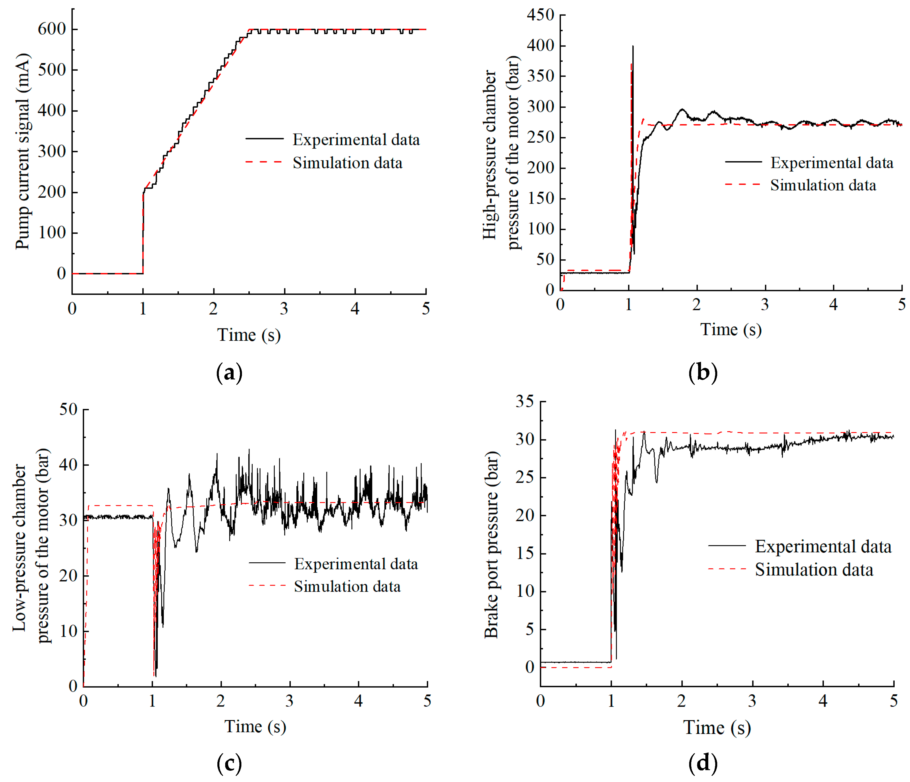
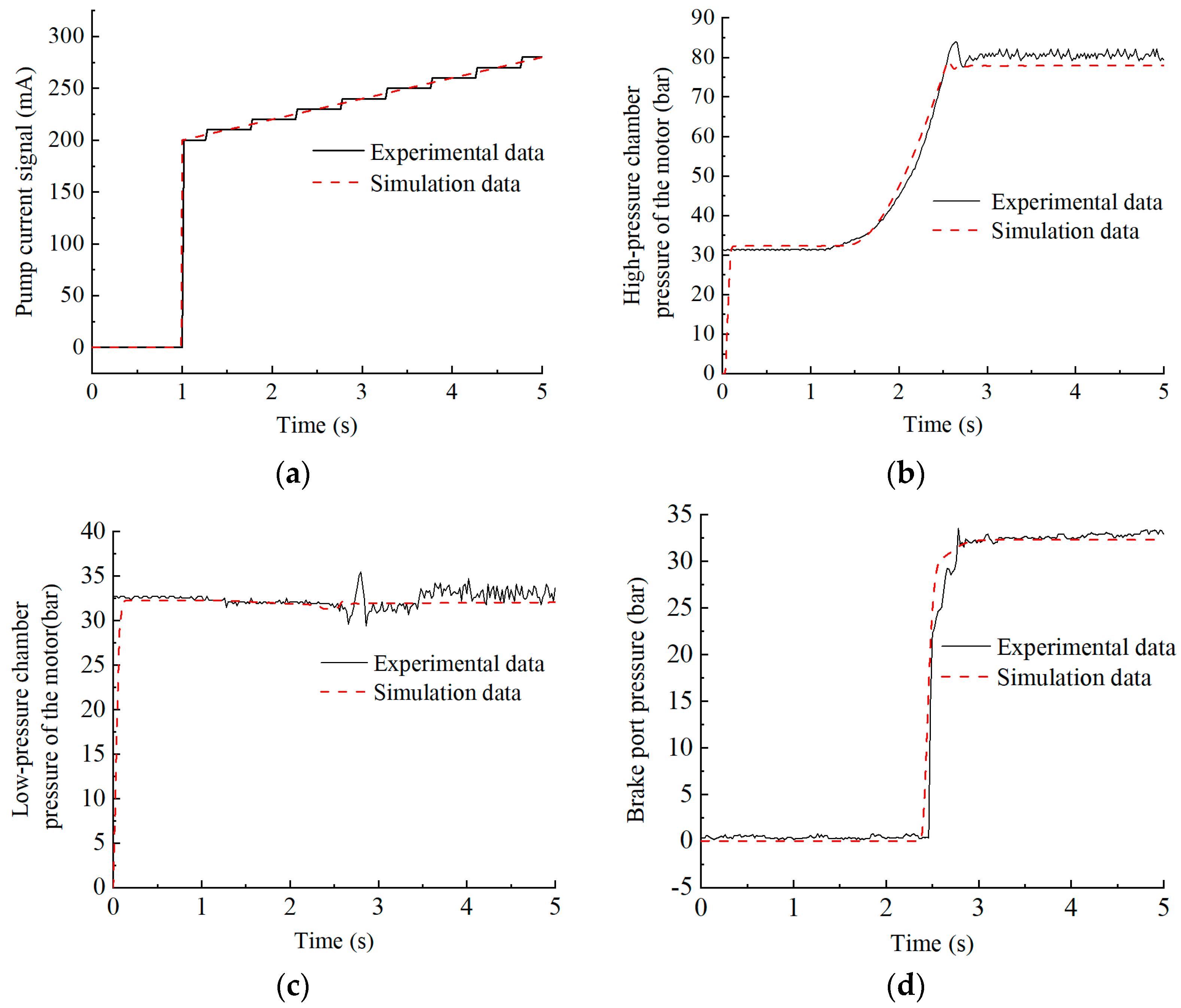
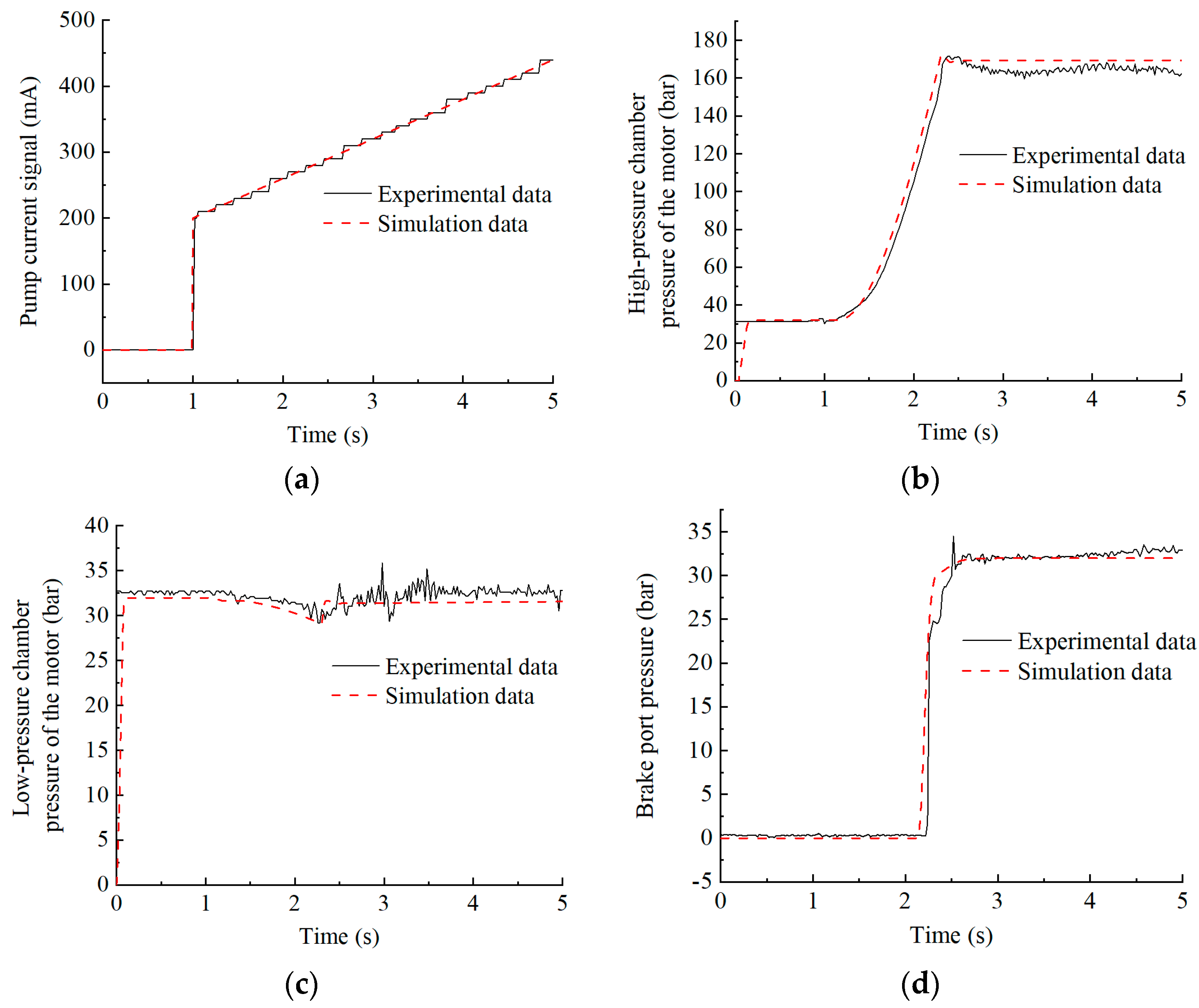
5.3. Experimental Test Analysis After Adding Control Strategy

According to the experimental principle and the experimental scheme of the secondary lifting action, the loads of 200 t and 600 t were tested, respectively. The initial state was 0.5 m from the ground, and the weight-lifting handle took 1.5 s to slowly push to the bottom. After some time, the handle slowly returned to the middle. It is worth noting that the push lifting handle is only used as a starting signal at this time, the controller will automatically perform a secondary lifting program, and the current signal of the input variable pump is given by the controller. When the load is 200 t, repeated experiments are carried out. After sorting out the collected experimental data, a better set of experimental results is obtained, as shown in Figure 23.

By comparing the simulation curve and the experimental curve of the 200 t load secondary lifting when using the control strategy, it can be seen that the trend of the simulation curve and the experimental test curve is the same.

From the experimental curve of Figure 23a, it can be seen that the second lifting action begins at 1 s, where the controller outputs the signal to the proportional valve of the variable pump and the displacement of the variable pump begins to increase from 0. Since the brake is not opened at this time, the motor is locked by the brake and has not yet rotated. From the experimental curves of Figure 23b,c, it can be seen that the pressure of the closed pipeline between the variable pump and the hydraulic motor begins to increase, and the pressure of the low-pressure chamber of the motor changes little. From the experimental curve of Figure 23d, it can be seen that the 2.5 s brake starts to open under the secondary lifting control strategy. At this time, the pressure of the high-pressure chamber of the motor is 67 bar, which is consistent with 70% of the steady-state pressure set by the control strategy. The high-pressure chamber of the motor reaches a maximum pressure of 83.5 bar at 2.7 s, and the overshoot is 2.5%, which meets the requirements of the secondary lifting performance optimization target. After the second lifting dynamic process, the pressure of the high-pressure chamber of the motor is stable at about 81 bar, the simulation model is 78 bar, and the gap between the simulation and the experimental test is only 3.8%.

When the load is 600 t, repeated experiments are carried out. After sorting out the collected experimental data, a better set of experimental results is obtained, as shown in Figure 24.

By comparing the simulation curve and the experimental curve of the 600 t load secondary lifting when using the control strategy, it can be seen that the trend of the simulation curve and the experimental test curve is the same.

From the experimental curve of Figure 24a, it can be seen that the second lifting action begins at 1 s, the controller outputs the signal to the proportional valve of the variable pump, and the displacement of the variable pump begins to increase from 0. Since the brake is not open at this time, the motor is locked by the brake and has not yet rotated. From the experimental curves of Figure 24b,c, it can be seen that the pressure of the closed pipeline between the variable pump and the hydraulic motor begins to increase, while the pressure of the low-pressure chamber of the motor gradually decreases. This is mainly because the flow of the oil pump is not enough to supplement the leakage flow and the flow required for the system to build pressure. After the system builds pressure, the pressure of the low-pressure chamber rises back to the normal oil supply pressure. It can be seen from the experimental curve in Figure 24d that at 2.34 s, the brake starts to open under the secondary lifting control strategy. At this time, the pressure of the high-pressure chamber of the motor is 122 bar, which is basically consistent with 70% of the steady-state pressure set by the control strategy. The high-pressure chamber of the motor reaches a maximum pressure of 167 bar at 2.62 s, and the overshoot is 3.7%, which meets the requirements of the secondary lifting performance optimization target. After the second lifting dynamic process, the pressure of the high-pressure chamber of the motor is stable at about 162 bar, the simulation model is 169 bar, and the gap between the simulation and the experimental test is only 4.1%.

In summary, after adding the control strategy, the error between the simulation data and the experimental test data is small, which can verify the accuracy of the simulation model and the rationality of the control strategy.

6. Discussion

This study presents an effective control strategy for preventing load slipping during secondary lifting in crawler cranes, caused by hydraulic motor reversal. By introducing a memory pressure algorithm, adjusting delay coefficients, and synchronizing motor pressure build-up with brake release, the proposed strategy ensures stability and smooth transitions during secondary lifting operations. The experimental results confirm that, with a delay coefficient of 0.70, no slipping occurred under load conditions ranging from 200 tons to 1000 tons. This approach not only resolves the issue of motor reversal, but also offers improved efficiency and reliability, making it suitable for large-scale applications. The potential for energy savings and economic benefits further strengthens the applicability of this method in real-world crane operations.

In

Table 5. Comparative table.

Contribution Area	Previous Works	Authors’ Proposal
Dynamic Control Strategies	Dynamic modeling and anti-sway control for vertical lifting of slender beam-shaped loads [18]; anti-sway positioning using sliding mode control [19]; time-optimal control for load sway suppression [20].	Focuses on secondary lifting challenges, addressing load slipping caused by motor reversal during lifting transitions.
Intelligent Algorithms	Utilization of LQR, fuzzy control, and neural network control to optimize crane lifting processes [23,24,25].	Incorporates a delay coefficient and pressure memory algorithm to achieve stability in secondary lifting operations.
Energy Recovery and Efficiency	Advanced energy recovery and position control strategies using neural networks and adaptive control [26,27,28].	Ensures no load slipping and minimizes system shocks under varying load conditions (200 t, 600 t, 1000 t).
System Stability and Safety	Enhanced safety in off-shore crane operations with cascaded NMPC-PID control strategies [27].	Provides theoretical guidance for stable and efficient operation of crawler crane secondary lifting systems.
Research Focus	Studies primarily address anti-sway control and dynamic modeling in cranes [12,13,14,15,16,17,18,19,20,21,22].	Highlights unique challenges of secondary lifting in large-tonnage crawler cranes, focusing on hydraulic control.

, we compare the main contributions of our research with those of previous works. As shown, our proposed secondary lifting control strategy, which incorporates a delay coefficient and pressure memory algorithm, significantly improves the system stability under varying load conditions, particularly when compared to previous studies that focused primarily on anti-sway control and dynamic modeling. These results emphasize the novelty of our approach in tackling the specific challenges of secondary lifting in crawler cranes.

7. Conclusions

Large crawler cranes play an increasingly important role in today’s engineering construction. As a lifting system that directly affects the overall performance of crawler cranes, their stability and safety are particularly important. As a common problem in the lifting system, secondary lifting and sliding have a great influence on the dynamic performance of the lifting system. The impact load generated is several times the lifting load, which seriously shortens the working life of the crawler crane and brings potential safety hazards to the construction operation. This paper takes the crawler crane as the research object, focuses on the analysis of the secondary lifting problem of the lifting system, and explores the dynamic characteristics of the secondary lifting of the lifting system. There are also significant advantages in terms of the process efficiency, energy savings, economic benefits, and streamlining the process. Aiming at the secondary lifting problem of the lifting system, the main research results of this paper are as follows:

(1)

The secondary lifting performance of the crawler crane is analyzed using an electromechanical–hydraulic co-simulation platform, and the control strategy, which can adapt to different weights, is designed to solve the problem of secondary lifting and sliding.

(2)

Aiming at the problem of secondary lifting and sliding, a control strategy is designed and simulated. The anti-interference ability is analyzed by using a no-delay coefficient and considering the starting time of the motor. The secondary lifting experiment of the crawler crane is carried out. The experimental research is carried out without a control strategy and after adding a control strategy. The accuracy of the electromechanical–hydraulic co-simulation model is verified by comparing the experimental results with the simulation results.

(3)

The experimental data show that the proposed control strategy can effectively solve the problem of secondary lifting and sliding and has a good dynamic performance. Under different load conditions of 200–1000 t, the secondary lifting and sliding phenomenon did not appear in the control strategy. The average starting time of the motor was 1.32 s, and the average overshoot of the high-pressure chamber pressure of the motor was 1.75%. After adding interference, there was no secondary lifting and sliding phenomenon, and the over-shoot of the high-pressure chamber pressure did not exceed 5%. The optimal control strategy is obtained when the optimal delay coefficient is 0.70.

References

1. Singhose, W. Command shaping for flexible systems: A review of the first 50 years. Int. J. Precis. Eng. Manuf. 2009, 10, 153–168. [Google Scholar] [CrossRef]
2. Li, Y.; Xi, X.; Xie, J.; Liu, C. Study and implementation of a cooperative hoisting for two crawler cranes. J. Intell. Robot. Syst. 2016, 83, 165–178. [Google Scholar] [CrossRef]
3. Ramli, L.; Mohamed, Z.; Abdullahi, A.M.; Jaafar, H.; Lazim, I.M. Control strategies for crane systems: A comprehensive review. Mech. Syst. Signal Process. 2017, 95, 1–23. [Google Scholar] [CrossRef]
4. Hu, S.; Fang, Y.; Bai, Y. Automation and optimization in crane lift planning: A critical review. Adv. Eng. Inform. 2021, 49, 101346. [Google Scholar] [CrossRef]
5. Zhang, S.; Minav, T.; Pietola, M.; Kauranne, H.; Kajaste, J. The effects of control methods on energy efficiency and position tracking of an electro-hydraulic excavator equipped with zonal hydraulics. Autom. Constr. 2019, 100, 129–144. [Google Scholar] [CrossRef]
6. Vaughan, J.; Singhose, W.; Kim, D. Analysis of unrestrained crawler-crane counterweights during tip-over accidents. Mech. Based Des. Struct. Mach. 2022, 50, 2006–2031. [Google Scholar] [CrossRef]
7. Ai, X.; Zsaki, A.M. Stability assessment of homogeneous slopes loaded with mobile tracked cranes—An artificial neural network approach. Cogent Eng. 2017, 4, 1360236. [Google Scholar] [CrossRef]
8. Zhao, J.; Wang, Z.; Yang, T.; Xu, J.; Ma, Z.; Wang, C. Design of a novel modal space sliding mode controller for electro-hydraulic driven multi-dimensional force loading parallel mechanism. ISA Trans. 2020, 99, 374–386. [Google Scholar] [CrossRef] [PubMed]
9. Hussain, M.; Ye, Z.; Chi, H.-L.; Hsu, S.-C. Predicting degraded lifting capacity of aging tower cranes: A digital twin-driven approach. Adv. Eng. Inform. 2024, 59, 102310. [Google Scholar] [CrossRef]
10. Gu, J.; Qin, Y.; Xia, Y.; Wang, J.; Gao, H.; Jiao, Q. Failure analysis and prevention for tower crane as sudden unloading. J. Fail. Anal. Prev. 2021, 21, 1590–1595. [Google Scholar] [CrossRef]
11. Fang, Y.; Wang, P.; Sun, N.; Zhang, Y. Dynamics analysis and nonlinear control of an offshore boom crane. IEEE Trans. Ind. Electron. 2013, 61, 414–427. [Google Scholar] [CrossRef]
12. Schlott, P.; Rauscher, F.; Sawodny, O. Modelling the structural dynamics of a tower crane. In Proceedings of the2016 IEEE International Conference on Advanced Intelligent Mechatronics (AIM), Banff, AB, Canada, 12–15 July 2016; pp. 763–768. [Google Scholar]
13. Zhao, Y.; Wu, X.; Li, F.; Zhang, Y. Positioning and swing elimination control of the overhead crane system with double-pendulum dynamics. J. Vib. Eng. Technol. 2024, 12, 971–978. [Google Scholar] [CrossRef]
14. Johns, B.; Abdi, E.; Arashpour, M. Dynamical modelling of boom tower crane rigging systems: Model selection for construction. Arch. Civ. Mech. Eng. 2023, 23, 162. [Google Scholar] [CrossRef]
15. Xin, Y.; Dong, R.; Lv, S. Dynamic Simulation Analysis of Truck Crane Based on ADAMS. Recent Pat. Mech. Eng. 2023, 16, 274–282. [Google Scholar] [CrossRef]
16. Li, G.; Ma, X.; Li, Z.; Guo, P.; Li, Y. Kinematic coupling-based trajectory planning for rotary crane system with double-pendulum effects and output constraints. J. Field Robot. 2023, 40, 289–305. [Google Scholar] [CrossRef]
17. Xia, M.; Wang, X.; Wu, Q. Modeling and anti-sway control method for vertical lift-up/lay-down process of slender-beam payload. ISA Trans. 2024, 149, 337–347. [Google Scholar] [CrossRef] [PubMed]
18. Wang, T.; Tan, N.; Zhou, C.; Zhang, C.; Zhi, Y. Anovel anti-swing positioning controller for two dimensional bridge crane via dynamic sliding mode variable structure. Procedia Comput. Sci. 2018, 131, 626–632. [Google Scholar] [CrossRef]
19. Takahashi, H.; Farrage, A.; Terauchi, K.; Sasai, S.; Sakurai, H.; Okubo, M.; Uchiyama, N. Sensor-less and time-optimal control for load-sway and boom-twist suppression using boom horizontal motion of large cranes. Autom. Constr. 2022, 134, 104086. [Google Scholar] [CrossRef]
20. Yang, C.; Du, C.; Liao, L. Design and implementation of finite time sliding mode controller for fuzzy overhead crane system. ISA Trans. 2022, 124, 374–385. [Google Scholar]
21. Lee, S.G. Modeling and advanced sliding mode controls of crawler cranes considering wire rope elasticity and complicated operations. Mech. Syst. Signal Process. 2018, 103, 250–263. [Google Scholar]
22. Rigatos, G. Nonlinear optimal control for the underactuated double-pendulum overhead crane. J. Vib. Eng. Technol. 2024, 12, 1203–1223. [Google Scholar] [CrossRef]
23. Cai, P.; Cai, Y.; Chandrasekaran, I.; Zheng, J. Parallel genetic algorithm based automatic path planning for crane lifting in complex environments. Autom. Constr. 2016, 62, 133–147. [Google Scholar] [CrossRef]
24. Cai, P.; Chandrasekaran, I.; Zheng, J.; Cai, Y. Automatic path planning for dual-crane lifting in complex environments using a prioritized multiobjective PGA. IEEE Trans. Ind. Inform. 2017, 14, 829–845. [Google Scholar] [CrossRef]
25. Jin, X.; Xu, W. Neural network based adaptive robust synchronous control of double-lift overhead crane considering input saturation. J. Frankl. Inst. 2024, 361, 106922. [Google Scholar] [CrossRef]
26. Chen, S.; Xie, P.; Liao, J. Cascade NMPC-PID control strategy of active heave compensation system for ship-mounted offshore crane. Ocean Eng. 2024, 302, 117648. [Google Scholar] [CrossRef]
27. Chen, S.; Xie, P.; Liao, J.; Wu, S.; Su, Y. NMPC-PID control of secondary regulated active heave compensation system for offshore crane. Ocean Eng. 2023, 287, 115902. [Google Scholar] [CrossRef]
28. Ranjan, P.; Wrat, G.; Bhola, M.; Mishra, S.K.; Das, J. A novel approach for the energy recovery and position control of a hybrid hydraulic excavator. ISA Trans. 2020, 99, 387–402. [Google Scholar] [CrossRef] [PubMed]
Figure 1. Schematic diagram of the 1250-ton crawler crane operation. A—Variable pump proportional valve current; P1—Motor high-pressure chamber pressure; P2—Motor low-pressure chamber pressure; P3—Brake port pressure.
Machines 13 00106 g001
Figure 2. Transfer function block diagram of lifting hydraulic system.
Machines 13 00106 g002
Figure 3. Secondary lifting action control strategy.
Machines 13 00106 g003
Figure 4. Crane simulation model.
Machines 13 00106 g004
Figure 5. Lifting system co-simulation model. 1—Electric proportional control variable pump; 2—Oil replenishment system; 3—AMESim–Simulink interface; 4—AMESim–ADAMS interface; 5—Switch valve group; 6—Brake; 7—Electric proportional control variable motor; 8—Explosion-proof valve.
Machines 13 00106 g005
Figure 6. Input current of variable pump without control strategy.
Machines 13 00106 g006
Figure 7. Motor speed curve without control strategy.
Machines 13 00106 g007
Figure 8. Pressure curve of the high-pressure chamber of the motor without control strategy.
Machines 13 00106 g008
Figure 9. Pressure curve of low-pressure chamber of the motor without control strategy.
Machines 13 00106 g009
Figure 10. Brake-opening process.
Machines 13 00106 g010
Figure 11. Pressure sensors at both ends of the motor.
Machines 13 00106 g011
Figure 12. (ac) Pressure curve of the high-pressure chamber.
Machines 13 00106 g012
Figure 13. (ac) Motor rotational speed curve.
Machines 13 00106 g013
Figure 14. (ac) Pressure curve of the low-pressure chamber.
Machines 13 00106 g014
Figure 15. (ac) Control strategy ahead by 70 ms.
Machines 13 00106 g015
Figure 16. (ac) Control strategy delay of 70 ms.
Machines 13 00106 g016
Figure 17. Experimental test of 1250 t crawler crane.
Machines 13 00106 g017
Figure 18. Appearance of the winch system.
Machines 13 00106 g018
Figure 19. Variable pump sensor installation.
Machines 13 00106 g019
Figure 20. Motor sensor installation.
Machines 13 00106 g020
Figure 21. Electrical control system.
Machines 13 00106 g021
Figure 22. Secondary lifting experimental curve without control strategy. (a) Variable pump displacement signal; (b) High-pressure chamber pressure of the motor; (c) Low-pressure chamber pressure of the motor; (d) Brake port pressure.
Machines 13 00106 g022
Figure 23. The 200 t load control strategy secondary lifting experimental curve. (a) Variable pump displacement signal; (b) High-pressure chamber pressure of the motor; (c) Low-pressure chamber pressure of the motor; (d) Brake port pressure.
Machines 13 00106 g023
Figure 24. The 600 t load control strategy to join the control strategy of secondary lifting experimental curve. (a) Variable pump displacement signal; (b) High-pressure chamber pressure of the motor; (c) Low-pressure chamber pressure of the motor; (d) Brake port pressure.
Machines 13 00106 g024