Multi-Stage Domain-Adapted 6D Pose Estimation of Warehouse Load Carriers: A Deep Convolutional Neural Network Approach

Abstract

Intelligent autonomous guided vehicles (AGVs) are of huge importance in facilitating the automation of load handling in the era of Industry 4.0. AGVs heavily rely on environmental perception, such as the 6D poses of objects, in order to execute complex tasks efficiently. Therefore, estimating the 6D poses of objects in warehouses is crucial for proper load handling in modern intra-logistics warehouse environments. This study presents a deep convolutional neural network approach for estimating the pose of warehouse load carriers. Recognizing the paucity of labeled real 6D pose estimation data, the proposed approach uses only synthetic RGB warehouse data to train the network. Domain adaption was applied using a Contrastive Unpaired Image-to-Image Translation (CUT) Network to generate domain-adapted training data that can bridge the domain gap between synthetic and real environments and help the model generalize better over realistic scenes. In order to increase the detection range, a multi-stage refinement detection pipeline is developed using consistent multi-view multi-object 6D pose estimation (CosyPose) networks. The proposed framework was tested with different training scenarios, and its performance was comprehensively analyzed and compared with a state-of-the-art non-adapted single-stage pose estimation approach, showing an improvement of up to 80% on the ADD-S AUC metric. Using a mix of adapted and non-adapted synthetic data along with splitting the state space into multiple refiners, the proposed approach achieved an ADD-S AUC performance greater than 0.81 over a wide detection range, from one and up to five meters, while still being trained on a relatively small synthetic dataset for a limited number of epochs.

1. Introduction

In the era of Industry 4.0, there is an ever-increasing demand for the autonomous handling of materials and goods in a warehouse. Intelligent autonomous guided vehicles (AGVs) for transportation will play a crucial role in the future of intra-logistics. Autonomous trucks carrying loads and performing difficult tasks with high efficiency and repeatability are a game changer in the intra-logistics industry [1,2].

The perception of the environment is an important element in AGVs to ensure safe, reliable, and flexible operation. This can be accomplished by equipping cars with assistive technologies such as various types of sensors, 2D/3D cameras, laser scanners, or radars. Deep learning algorithms are used to extract information about the surrounding and contents of the warehouse based on sensor measurement data [3,4]. With these data, the AGV can navigate, map, and perform loading and unloading duties safely in the warehouse. For warehouse load carriers completing a loading task through an intelligent AGV, it is better to divide this complex task into several sub-tasks. Navigation and docking represent the first sub-task, and they involve localization, collision avoidance, and trajectory planning. Perception is the second sub-task, which can be divided into two parts: object detection and 6D pose estimation. The 6D pose estimation task is the main focus of this study. In this regard, the object’s 6D pose is parameterized by the roll, pitch, and yaw rotational angles in addition to translations in the x, y and z axes. More specifically, the interest is in estimating the poses of warehouse load carriers relative to AGVs. Since the camera collecting the images is mounted on the AGV, the task can be specified as estimating the pose of the load carrier relative to the camera frame, as seen in Figure 1.

In this work, we develop a deep learning-based framework for 6D pose estimation of warehouse load carriers using RGB information only. The framework is composed of a domain adaptation network and a multi-stage pose estimation and refinement network. It is also modular and does not rely on a strict architecture design to ensure flexibility. The framework relies on only synthetic data for training and was evaluated using real warehouse data on both close and far away objects (in the range of 1–5 m).

The structure of this work is organized as follows: Section 2 provides the necessary background and problem statement for the work. Section 3 goes through the dataset collection and generation process and provides information on the datasets used in this work. In Section 4, the methodology for developing the proposed multi-stage domain-adapted pose refinement pipeline is explained. In Section 5, the results are demonstrated and discussed. Finally, conclusions are drawn in Section 6 along with suggestions for future work.

2. Background and Problem Statement

2.1. The Use of Synthetic Data for Training Convolutional Neural Networks

Industrial models must be stable and generalizable in a variety of situations before they can be deployed. Deep networks have advanced rapidly in recent years, making it possible to train a model for a variety of tasks with enough annotated data. However, the process of obtaining and annotating large datasets can be costly, time-consuming, and labor-intensive, as well as prone to human error in the case of manual data labeling. It is common to use computer simulations and graphics to collect annotated data in large quantities with little computational time and effort to facilitate the data collection process. The disadvantage is that the simulated synthetic data does not appear realistic, as seen in Figure 2, resulting in a domain gap between the real and synthetic domains. The term “domain gap” refers to the poor transferability of deep neural network perception models. The domain gap between the synthetic and actual domains would cause a model that performs well on the synthetic domain to perform significantly worse on real data scenarios.

Producing realistically rendered synthetic scenery would decrease the domain gap; however, it would increase the effort put into generating each dataset or scenery, making the easy data generation method lose its essence [5]. Another solution is to use domain randomization [6], where objects are rendered with randomized backgrounds, lighting conditions, materials, and other parameters, as seen in Figure 3. However, using domain randomization is usually not sufficient, and it is often necessary to combine the domain-randomized data with more realistic-looking data [7].

2.2. Domain Adaptation Networks

Another approach to solving the domain gap problem can be achieved by using domain adaptation techniques. Domain adaptation is a type of transfer learning, where the model learns information from a source domain (the synthetic domain) in order to perform well on a related yet different target domain (the real domain).

In [8], an Image-to-Image Translation domain adaptation network named CycleGAN was developed. The network consists of two generators, where the first maps input images from domain A to domain B, while the second generator maps the input images from domain B back to domain A. The cyclic adversarial network relies on the cycle-consistency loss, which is computed as the difference between the input image to the first generator and the output of the second generator. However, the network does not ensure semantic consistency for images before and after adaptation and requires two generators and discriminators, significantly increasing the computational requirements.

In [9], a semantic-consistency loss in addition to the cycle-consistency loss was used for the Image-to-Image Translation domain adaptation task. The semantic-consistency loss computes the difference between the predicted semantic labels before and after adaptation. However, the model requires training a semantic segmentation network in addition to using two generators and two discriminators, increasing computational efforts. The network is named cycle-consistent adversarial domain adaptation or CyCADA for short.

A Network named Contrastive Learning for Unpaired Image-to-Image Translation or CUT for short was developed in [10]. The network is an Image-to-Image Translation domain adaptation network that relies on contrastive loss, where corresponding parts of the image before and after translation/adaptation are encouraged to be mapped to similar points in the latent space. This approach allows the network to preserve semantic consistency by maximizing the mutual information between images before and after translation/adaptation. One of the main advantages of the network is its requirement of only one generator and discriminator.

In [11], a novel diffusion-based cross-domain image translator named CycleDiff was developed. This approach integrates diffusion models to learn the image translation process without requiring paired training data. CycleDiff employs a joint learning framework that aligns the diffusion and translation processes, enhancing global optimality and improving fidelity and structural consistency.

In [12], Dual Diffusion Implicit Bridges (DDIBs) were introduced as an image translation method based on diffusion models. DDIBs circumvent the need for paired training on domain pairs by using two diffusion models independently trained on each domain. The translation process involves obtaining latent encodings from the source images with the source diffusion model and decoding them using the target model to construct the target images.

In [13], a method named CycleGAN-Turbo was introduced to enhance Image-to-Image Translation tasks. This approach consolidates the modules of a vanilla latent diffusion model into a single end-to-end generator network, reducing overfitting and preserving the input image structure. CycleGAN-Turbo outperforms existing GAN-based and diffusion-based methods in unpaired settings, such as day-to-night conversion and weather-effect modifications, by using adversarial learning objectives.

In [14], the CycleVAR approach was introduced to enhance Image-to-Image translation tasks by incorporating variational autoencoder (VAE) quantization and autoregressive transformer-based generation. CycleVAR differentiates itself from CycleGAN by utilizing variational autoencoders (VAEs) for quantization, which allows for more efficient encoding of image data into discrete latent spaces. Additionally, CycleVAR employs an autoregressive transformer-based generation mechanism, which enhances the model’s ability to generate high-quality images by sequentially predicting pixel values.

Although Unparied Image-to-Image Transslation (UNIT) approaches like CUT were used for domain adaptation in semantic segmentation tasks, these approaches were not evaluated to bridge the synthetic–real domain gap in 6D object pose estimation tasks. If Image-to-Image Translation domain adaptation techniques were able to minimize the synthetic–real domain gap, then the significance of the photorealism in produced synthetic data would decay. The result would be producing synthetic data more easily with less worries about photorealsim, leading to an easier 6D object pose estimation task.

2.3. Deep Learning Approaches for 6D Pose Estimation

Deep learning approaches and Convolutional Neural Networks (CNNs) have recently shown superior performances in pose estimation compared to classical computer vision techniques. Most importantly, they have shown an excellent ability to deal with textureless objects and occluded scenes, which were a major limitation for template- and feature-matching approaches used in classical computer vision applications [15,16].

PoseCNN was introduced by [17] as one of the first deep CNNs to estimate the 6D poses of objects. PoseCNN uses CNNs for feature extraction. PoseCNN introduces a shape-matching loss that is able to deal with symmetries by computing the distance between each point of the predicted object’s pose and its closest point on the ground-truth pose model. However, the performance of PoseCNN is very modest with a high inference time.

In Deep Object Pose Estimation (DOPE) [7], keypoints are detected using a fully convolutional network, and pose solutions are solved using the Efficient-Perspective-n-Point (EPnP) solver [18]. DOPE was the first 6D pose estimation network trained using only synthetic data. Even though DOPE finds difficulties in handling symmetries, it was a major leap conveying the possibility of using synthetic data only for training pose estimation networks.

Instead of directly predicting the keypoints of the object, the Pixel-wise Voting Network (PVNet) [19] predicts unit vectors pointing towards the keypoints of the object. The unit vectors are then used in a Random Sample Consensus (RANSAC)-based voting scheme to obtain the keypoints of the object in addition to the uncertainty associated with each keypoint [20]. Afterward, a modified version of EPnP [18] can be leveraged to solve the 6D pose of the object. The PVNet approach yields good results and was even well evaluated on photorealistic synthetic data in the Benchmark Competition for the Estimation of the Pose of 6D Objects (BOP20) [21].

Six-dimensional Object Pose Estimation under Hybrid Representations (HybridPose) [22] introduced a hybrid representation by predicting keypoints in a similar manner to PVNet, in addition to edge vectors and symmetry correspondences. To solve for 6D poses, HybridPose uses a modified EPnP [18] model suitable for the hybrid representation. Additionally, a refinement sub-module is used as well to enhance the results. These modifications in HybridPose enhance the results over PVNet. However, the inference time increases drastically, and HybridPose still finds difficulty dealing with small objects. Moreover, HybridPose did not take place in BOP20 and was not evaluated with only synthetic data for training.

You Only Look Once 6D (YOLO6D) [23] estimates keypoints for multiple objects in a single shot, making the network fast and unaffected by the number of objects. The 6D pose in YOLO6D is then retrieved using the EPnP solver. The downside is that YOLO6D’s results are very modest, and they have not been evaluated when trained using only synthetic data, but with its reasonably low inference time, it is possible to combine YOLO6D with another pose refiner.

Using the RANSAC and PnP solvers as a PnP alternative degrades the speed of inference and makes the pipeline not end-to-end trainable. Therefore, Hu et al. [24] developed an artificial neural network (ANN) solver to overcome these limitations. The ANN-based solver was able to boost PVNet’s results in addition to decreasing the inference time. However, it was not evaluated with synthetic training data.

Deep Iterative Matching (DeepIM) [25] is a pose-matching refining network. In DeepIM, a high-resolution zoom-in strategy was introduced, making the refinement process possible even for small or very far objects. DeepIM [25] also introduces a reliable disentangled transformation representation, and the model can function as a tracker and a refiner. However, DeepIM was neither tested for initialization nor evaluated when trained only on synthetic data.

Consistent multi-view multi-object 6D pose estimation (CosyPose) [26] is a DeepIM-based refiner network with several enhancements and can be used to initialize 6D poses. Moreover, CosyPose was evaluated on various datasets when trained using photorealistic rendered data in BOP20, in addition to winning five awards in BOP20, including the best overall method and the best RGB-based pose estimation method. CosyPose uses a similar zoom-in procedure and a similar disentangled transformation representation to what was used in DeepIM.

Shape-Constraint Recurrent Flow (SCFlow) [27] introduces a novel end-to-end recurrent matching framework for 6D object pose estimation that explicitly incorporates 3D shape constraints into the pose refinement process. Unlike previous methods that rely on generic optical flow, SCFlow computes a pose-induced flow based on the displacement of 2D reprojections between the initial and estimated poses, effectively embedding the object’s shape into the matching process. This approach significantly reduces the matching space and improves learning efficiency.

RNNPose [28] presents a recurrent neural network-based framework for 6D object pose refinement that alternates between correspondence field estimation and pose optimization. The method formulates pose refinement as a non-linear least-squares problem, which is solved via a differentiable Levenberg–Marquardt algorithm, allowing for end-to-end training. Crucially, RNNPose introduces a descriptor-based consistency-check mechanism to handle occlusions by downweighting unreliable correspondences during optimization. Additionally, a 3D-2D hybrid network is used to generate distinctive descriptors for both the object model and the observed images.

NeRF-Pose [29] proposes a weakly-supervised, first-reconstruct-then-regress approach for 6D pose estimation. Unlike traditional methods requiring complete 3D CAD models and accurate 6D pose annotations, NeRF-Pose operates with only 2D bounding boxes and relative camera poses as weak supervision. The method first reconstructs the object’s implicit 3D representation using Neural Radiance Fields (NeRFs), and then trains a pose regression network to predict dense 2D-3D correspondences. During inference, the NeRF-enabled PnP+RANSAC procedure estimates the final pose from the correspondences.

SurfEmb [30] introduces the concept of learning dense and continuous 2D-3D correspondence distributions for object pose estimation without explicit supervision of visual ambiguities such as symmetry or occlusion. Utilizing a contrastive learning framework, SurfEmb represents dense correspondence distributions in an object-specific latent space, enabling the model to implicitly capture multi-modal surface correspondences. The method samples, scores, and refines pose hypotheses using these distributions, bypassing the need for explicit symmetry handling or handcrafted correspondences.

MRC-Net (MultiScale Residual Correlation Network) [31] proposes a single-shot, two-stage pipeline for 6D pose estimation from a single RGB image with a known 3D model. The first stage classifies the coarse pose and renders the object; the second stage regresses the fine-grained residual pose within the classified bin. A novel MultiScale Residual Correlation (MRC) layer connects the two stages, capturing detailed correspondences between the input and rendered images at multiple scales. Soft probabilistic labels are used to handle symmetries in the pose classification. MRC-Net is end-to-end trained and does not require iterative refinement or post-processing.

In pose estimation problems, it is common to use pose initialization methods or coarse models that estimate a 6D pose from an image without the need for an initial pose estimate, where an image is input into the network to obtain a coarse pose estimate directly. However, it is also possible to input an image in addition to the corresponding coarse estimate (initial pose) into a second pose estimation model to improve the initial pose estimations through iterative refinement; such a model is called a refiner. In addition to the superior performance of CosyPose networks compared to other state-of-the-art networks [32], a primary advantage of this network is that it can be used for both pose initialization and iterative pose refinement, providing additional flexibility for practical applications.

2.4. Problem Statement and Contribution

Previous studies in deep learning 6D pose estimation focused on datasets with the maximum depth not exceeding 1 m [17,33]. However, in load-carrier settings, the 6D poses should be practically determined from small (less than 1 m) and far distances (up to 5 m). This would require training the neural network with a very large amount of data for a very long time. Therefore, we propose dividing the state space into multiple slices using multiple refiners, where each refiner is trained on a slice of the space in a divide-and-conquer scheme. This enables the model to deal with close and far objects with minimal amount of training.

Additionally, previous work focused on using real or a mixture of real and (non-adapted) synthetic data for pose estimation networks. Recognizing the difficulties of obtaining real, 6D pose annotated data, the proposed framework uses only synthetic data along with domain adaptation using Image-to-Image Translation networks to bridge the domain gap between synthetic and real data.

Overall, we propose a pose estimation framework composed of a domain adaptation network and a multi-stage 6D pose estimation network that is modular and flexible, relies on RGB synthetic data, and is suitable for near and far objects. As a representative case study, the proposed framework is applied to the problem of 6D pose estimation of standard industrial pallets in an intra-logistics environment.

3. Warehouse Pose Estimation Datasets

In this study, we utilized multiple synthetic datasets to train our 6D pose estimation models and a real dataset to evaluate them. The data collection and generation processes involve capturing images with an RGB-D camera system and using a Vicon Motion Capture system for precise 6D pose annotations. This provides the ground-truth poses for the real-world dataset, enabling the evaluation of our models. The synthetic datasets, on the other hand, are generated using the NVIDIA Deep Learning Dataset Synthesizer (NDDS) version v1.0 and Unreal Engine version 4.22 [34], which randomize lighting conditions, object properties, and camera poses to simulate different environments.

3.1. Real Single-Pallet Pose Dataset (RPP)

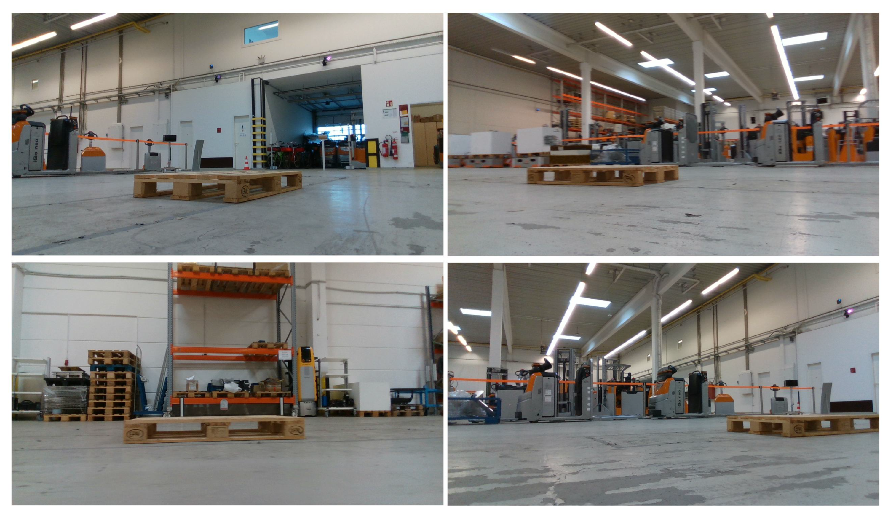
This dataset consists of 3.2k ($1280\times 720$) images, with the depth images available in addition to poses. Only a single pallet is annotated (pose) in this dataset, and therefore, it is named the Real Single-Pallet Pose dataset or the RPP dataset for short. Four samples of the dataset is displayed in Figure 4. This dataset is only used for testing.

3.2. Warehouse Synthetic Single-Pallet Pose Dataset (WSPP)

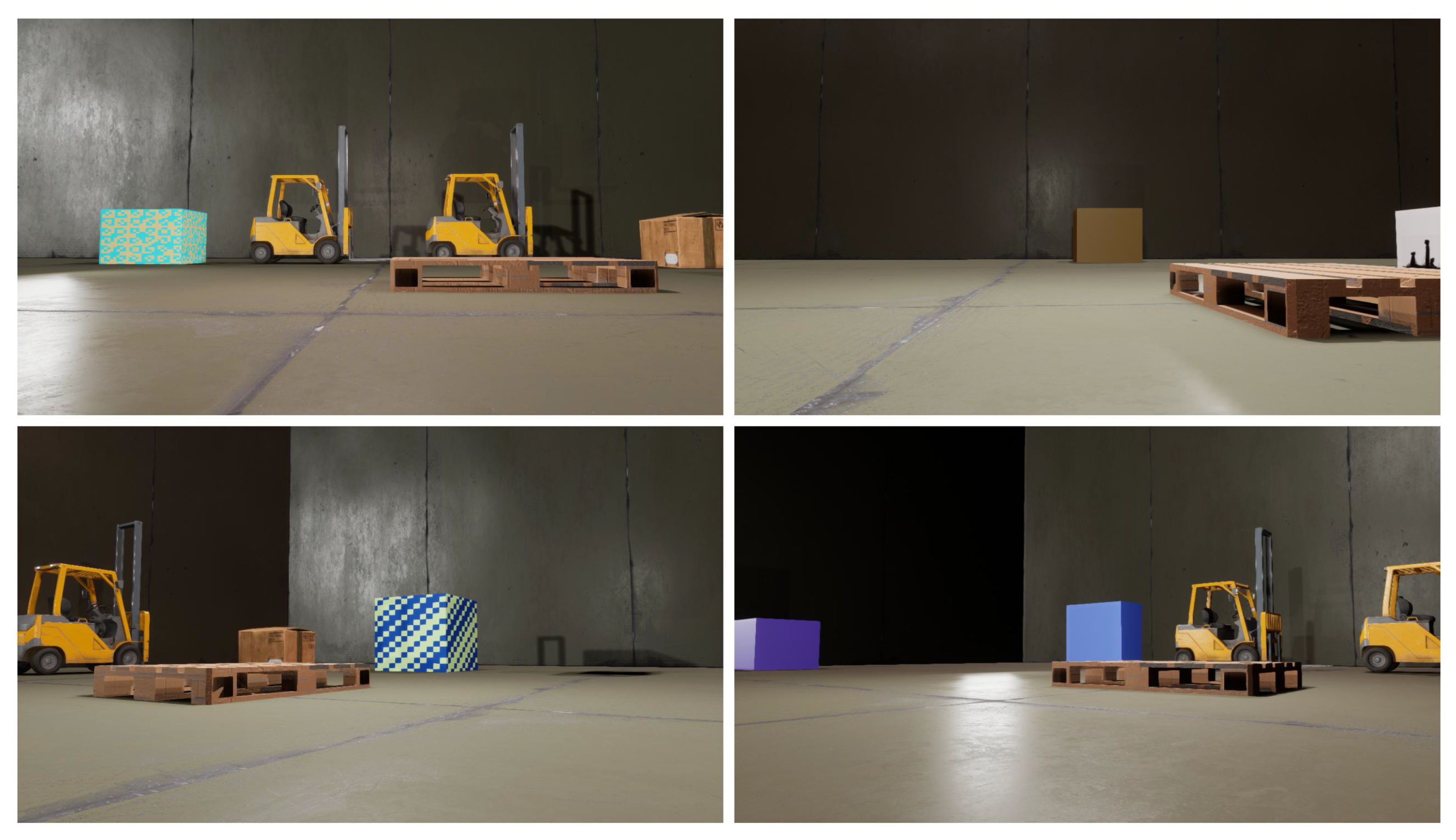
This dataset includes images from a camera orbiting around a pallet from several distances and angles. The lighting conditions are randomized, yet the floor and background are not. As simulated in Figure 5, the dataset includes randomized boxes in addition to forklifts. This dataset is called Warehouse Synthetic Single-Pallet Pose data, or WSPP for short. The dataset has 55k ($1280\times 720$) images, where 6D poses and keypoints are recorded. The dataset is split into two parts: A total of 50k images are used for training, and the remaining 5k images are used for validation.

3.3. Randomized Synthetic Single-Pallet Pose Dataset (RSPP)

The second of the two synthetic pose datasets is named Randomized Synthetic Single-Pallet Pose data or RSPP for short. This dataset has no objects other than a floating randomized pallet, while the camera rotates around it at various distances and angles. Both lights and backgrounds are randomized in this dataset. Similar to the WSPP dataset, the RSPP dataset has 55k ($1280\times 720$) images that are split into two parts: A total of 50k images are used for training, and the remaining 5k images are used for validation. The dataset is visualized in Figure 6.

4. Methodology

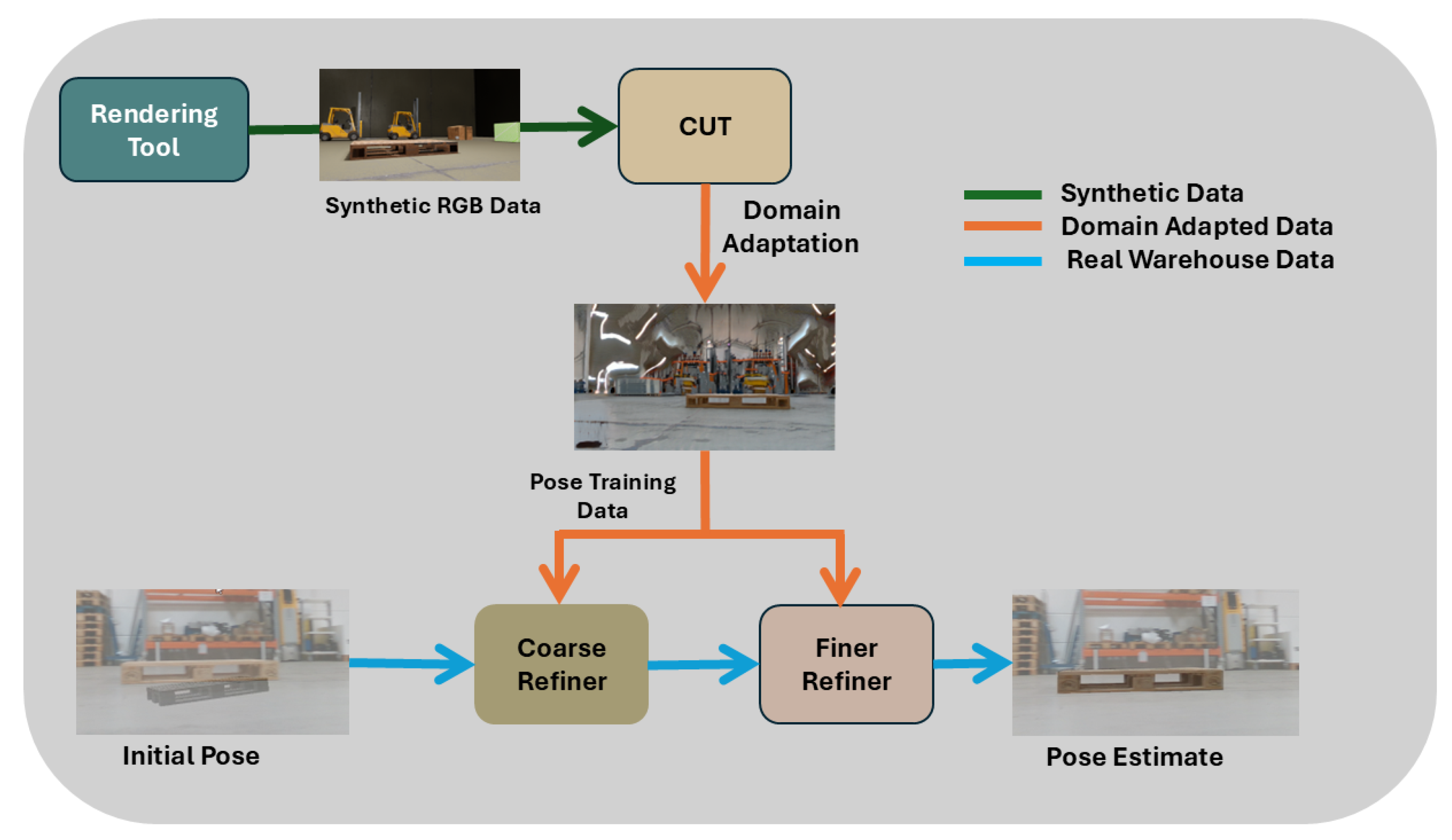
A flowchart that illustrates the proposed approach is shown in Figure 7.

4.1. CUT Network

In this work, we leverage the CUT Unpaired Image-to-Image Translation (UNIT) network to adapt synthetic warehouse data [10]. CUT is used as the domain adaptation network to bridge the gap between the synthetic and real domains. The choice of the CUT UNIT network for domain adaption is based on computational considerations with respect to the architecture of this GAN (includes one generator and one discriminator only), as well as its proven robustness in preserving semantic consistency between images before and after translation in semantic segmentation tasks. More details on the design and architecture of the CUT UNIT network can be found in [10].

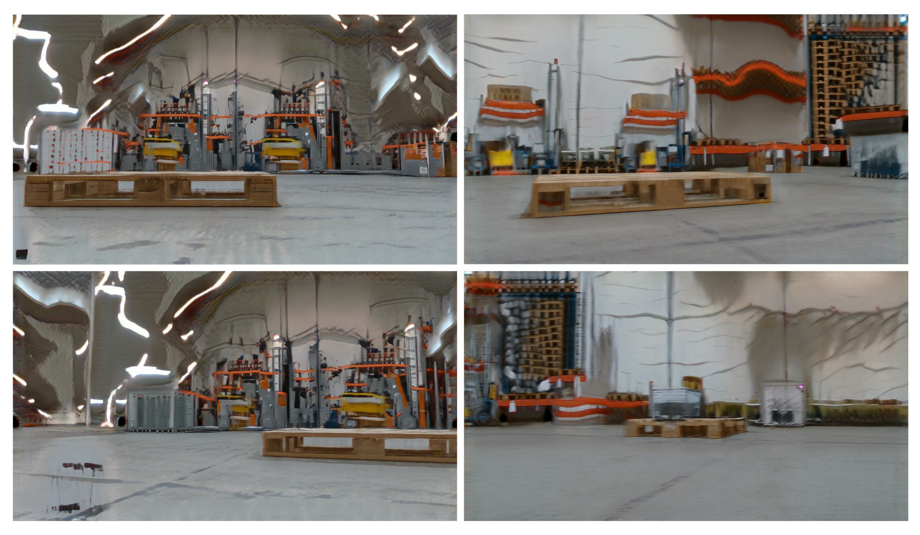
CUT is trained on 500 images from the WSPP dataset and 350 images from the RPP dataset. The network is trained to adapt the synthetic images from the WSPP dataset into the real domain of the RPP dataset, as shown in Figure 8. The images are resized into square ($600\times 600$) images, and a random crop is taken and input into the network. The resulting dataset from adapting the WSPP dataset is referred to in the manuscripts as the adapted-WSPP dataset. This dataset has 55k adapted images with dimensions of $1280\times 720$, from which 50k images are used for training training, while the remaining 5k are used for validation. Four samples of this dataset are displayed in Figure 9.

Table 1. Warehouse pose estimation datasets.

Dataset	Resolution	Training Size	Validation Size	Test Size	Synthetic	Real
RPP	$1280\times 720$	-	-	$3.2$k	✕	✓
WSPP	$1280\times 720$	50k	5k	-	✓	✕
RSPP	$1280\times 720$	50k	5k	-	✓	✕
Adapted-WSPP	$1280\times 720$	50k	5k	-	✓	✕

presents a summary of all warehouse pose estimation datasets, including the resolution and size of each dataset in addition to whether the dataset is synthetic or contains real images.

It is worth mentioning that the use of domain adaptation using the CUT Unpaired Image-to-Image Translation (UNIT) network in the proposed 6D pose estimation framework can be completely applied as a preprocessing step for the input image data to prepare the image inputs for the pose estimation network training, achieving a 6D pose estimation framework that is both modular and flexible.

4.2. Pose Estimation Network

The focus of this study is to design a multi-stage domain-adapted 6D pose estimation framework that is both trainable using only synthetic data and suitable for industrial applications. Additionally, the focus is on developing a generalizable framework that could be executed without heavy restrictions on the network design. Therefore, instead of designing a domain-specific pose estimation network, we leveraged a backbone CNN architecture from the literature to develop the proposed framework. In this study, we considered the CosyPose network as a backbone for the proposed multi-stage domain-adapted 6D pose estimation framework [26]. The choice for this backbone is based on the consistent excellent performance of this network over various datasets in the BOP20 challenge on 6D object localization [21]. More details on the design and architecture of the CosyPose refiner can be found in [26].

In this section, we present the proposed 6D pose multi-stage pipeline for 6D pose estimation and refinement. To perform a comprehensive evaluation, we also compared the proposed approach with the single-stage pipeline, which represents the state-of-the-art approach for 6D pose estimation. Moreover, to show the improvement obtained with domain adaptation in the proposed framework, we consider different training scenarios with respect to the choice of data to train each of these pipelines based on the WSPP, RSPP, and Adapted-WSPP datasets listed in Table 1. In order to simulate real-world uncertainty, the training scenarios also incorporate adding noise to the ground-truth poses during training to ensure that the developed pose estimation pipelines are able to handle noisy inputs. Finally, these pipelines are evaluated on the real warehouse dataset (RPP). Performance is then analyzed with respect to the accuracy of pose estimates predicted by these pipelines as well as the effectiveness of these pipelines in handling varying noise levels, focusing on the translational and rotational errors in predicted pose estimates of the real testing dataset.

4.2.1. Baseline: Single-Stage Pose Estimation and Refinement Pipeline

First, we considered building a baseline network of a single-stage CosyPose refiner such that it takes an initial pose estimate as input and outputs a refined pose. We considered evaluating three different scenarios with regard to the choice of the data to train the single-stage pose refinement pipeline.

Following [26], the refiner is trained using labeled synthetic data by inputting the ground-truth pose with additive noise sampled from a normal distribution ($\epsilon$∼$\mathcal{N}(Mean,STD)$), as visualized in Figure 10.

The noise-sampling process ensures randomness in the training input samples and results in better generalization while reducing the network’s likelihood of overfitting. The normal distributions’ parameters used in training the refiner network are displayed in

Table 2. Sampled noise to train the single-stage refiner.

	(cm)			(deg)
	x	y	z	Roll	Pitch	Yaw
Mean	0	0	0	0	0	0
STD	30	30	30	15	15	15

. The noise added in translation in the directions of the x, y, and z axes is sampled from normal distributions with a standard deviation of 0.3 m and a mean of zero ($\epsilon$∼$\mathcal{N}(0,0.3\mathrm{m})$). The added noise for roll, pitch, and yaw is sampled from normal distributions with 15 degrees of standard deviation and a mean of zero ($\epsilon$∼$\mathcal{N}(0,{15}^{\circ })$).

The three scenarios for training the single-stage refinement pipeline are shown in Figure 11 and can be summarized as follows:

(a)

Single-Stage Scenario-1: Basic Refiner

The first trained model is a basic refiner that is trained on 50k images from RSPP.

(b)

Single-Stage Scenario-2: WSPP Refiner

Retraining the basic refiner using 50k additional images is expected to enhance its performance even if the data was not adapted. To ensure that the adaptation enhances the performance more than just retraining using additional non-adapted synthetic data, WSPP data is used to re-train the CosyPose refiner along with the original 50k images from RSPP. This refiner, which is trained on non-adapted WSPP data, is named the WSPP refiner.

(c)

Single-Stage Scenario-3: Adapted Refiner

The CosyPose model is trained again using the 50k adapted-WSPP images (Section 4.1) in addition to the 50k images from RSPP. This model aims at showcasing the ability of the domain adaptation approach in enhancing its performance when no real labeled data is available for training. This refiner is referred to in the paper as the adapted refiner.

4.2.2. The Proposed Multi-Stage Pose Estimation and Refinement Pipeline

In this study, multi-stage pose refinement is proposed for enhancing pose estimation by adding a finer refiner after the first refiner network. The finer refiner is the CosyPose refiner that is trained in a similar scheme to the basic refiner explained in Section 4.2.1 using RSPP data. Similar to the first refiner, noise sampled from a normal distribution is added the ground-truth poses, as seen in Figure 10. However, the sampled noise’s standard deviation for the second refiner must be smaller in order to allow the finer refiner to refine the outputs of the basic refiner. The parameters of the normal distributions for training the finer refiner are shown in

Table 3. Sampled noise to train the finer refiner network.

	(cm)			(deg)
	x	y	z	Roll	Pitch	Yaw
Mean	0	0	0	0	0	0
STD	1	1	5	5	5	5

.

Two scenarios for the multi-stage refinement pipeline were considered to demonstrate the performance enhancement achieved in multi-stage domain-adapted pose estimation compared to multi-stage pose estimation without domain adaption. Both scenarios are illustrated in Figure 12.

(a)

Multi-stage Refinement Scenario-1: Basic + Finer

The first multi-stage model is constructed by adding the finer refiner after the basic refiner, as shown in Figure 12a. The initial pose estimate is refined first by the basic refiner for 2 iterations, as this provides an excellent trade-off between performance and inference speed. Afterwards, the pose is refined again for 4 iterations by the finer refiner. The intuition is that the finer refiner should be able to refine the small pose errors that the basic refiner was unable to enhance.

(b)

Multi-stage Refinement Scenario-2: Adapted + Finer

This modeling scenario uses the adapted refiner developed in Section 4.2.1 followed by a finer refiner, as shown in Figure 12b, to enhance the overall performance of the multi-stage pose refinement pipeline. Similarly to the first multi-stage scenario, the pose estimate is refined for two iterations using the adapted refiner, and then refined again for four iterations by the finer refiner.

4.3. Performance Analysis on the Real Test Dataset (RPP)

All trained refiner models were evaluated via performance analysis and comparisons on the real RPP test dataset. Also, to evaluate the ability of these models to deal with varying noise levels in testing data, noise is sampled from normal distributions and is added to ground-truth poses in RPP data to form initial pose estimates (similar to the process explained in Section 4.2 but this time applied to the real testing data under various noise settings).

In a warehouse setting using RGB images, the primary sources of error in 6D pose estimation are related to the depth (which we define as the z-axis) and the yaw angle. The difficulty in accurately estimating depth from RGB images contributes significantly to the error obtained. Depth estimation is inherently challenging, as RGB images lack direct depth information, making it harder to estimate the true 3D position of objects.

In addition, pallets in such settings are often placed on racks or directly on the floor. This positioning results in pitch and roll variations that are less significant compared to variations in the yaw angle. The yaw angle, which represents the rotational orientation of the object in the horizontal plane, is more prone to errors and fluctuations in these scenarios, thus having a greater impact on the accuracy of pose estimation.

Given these challenges, the focus of comparison in our analysis centers on the impact of noise on depth estimation and yaw angle variation. Specifically, we examine how changes in the level of noise in both of these factors affect the pose estimation results. By varying the noise levels in depth and yaw, we assess the robustness of the framework under different error conditions, which are typical in real-world warehouse environments. Therefore, two experiments were designed and performed to analyze the robustness of the refiner models against varying levels of noise in the initial pose estimates of the yaw rotational angle and depth. The standard deviation values used for noise with normal distributions for both experiments are displayed in

Table 4. Sampled noise to evaluate different refinement pipelines using RPP data.

Exp.	STD (cm)			STD (deg)
	x	y	z	Roll	Pitch	Yaw
1	30	30	10–100	15	15	15
2	30	30	30	15	15	15–45

. In Experiment 1, the standard deviation of the noise distribution in the z-axis (depth) is varied, while the standard deviation of the noise distribution of the yaw angle is varied in Experiment 2. In both experiments, the noisy pose inputs are refined in four iterations.

4.4. Evaluation Metrics

The symmetric average distance (ADD-S ) metric [35] computes the average distance between the model’s 3D points ($i\in X_Q$) transformed according to the predicted pose ($\widehat{T}$) and the ground-truth (T) pose based on the closest point:

$$\mathrm{ADD}\text{-}\mathrm{S}={\displaystyle \frac{1}{\parallel X_Q\parallel }}\sum _{i\in X_Q}\underset{j\in X_Q}{min}\parallel \widehat{T}j-Ti\parallel ,$$

(1)

where $\parallel X_Q\parallel$ is the number of 3D model points (cardinality). Moreover, accuracy can be computed as the ratio between prediction with ADD-S scores below a specific threshold and the total number of ground-truth predictions. In [17] it was suggested to take the area under the accuracy–threshold curve (AUC) as a metric (ADD-S AUC). The threshold in the accuracy–threshold curve varies between 0 to 10 cm [17,36].

The ADD-S AUC is given by

$$\mathrm{ADD}\text{-}\mathrm{S}\mathrm{AUC}={\int }_0^{10}\mathrm{Accuracy}\left(t\right)dt$$

(2)

where $\mathrm{Accuracy}\left(t\right)$ is the accuracy computed at each threshold t, which is the fraction of predictions for which the ADD-S score is below the threshold t. The AUC metric aggregates performance across various thresholds, providing a more robust evaluation of the model’s ability to estimate poses within different tolerances.

The Mean Absolute Error (MAE) can be used to compute errors for both translation (in the x, y, and z axes) and rotation (in the roll, pitch, and yaw axes). This error metric is computed as shown below.

For translation, let x, y, and z represent the ground-truth translation values in the x, y, and z axes, and let $x_p$, $y_p$, and $z_p$ represent the predicted translation values for each axis. The MAE for each axis of translation is computed as the absolute difference between the predicted and ground-truth values:

$${\mathrm{MAE}}_x={\displaystyle \frac{1}{N}}\sum _{i=1}^N\left|x_i-x_{p_i}\right|$$

(3)

$${\mathrm{MAE}}_y={\displaystyle \frac{1}{N}}\sum _{i=1}^N\left|y_i-y_{p_i}\right|$$

(4)

$${\mathrm{MAE}}_z={\displaystyle \frac{1}{N}}\sum _{i=1}^N\left|z_i-z_{p_i}\right|$$

(5)

where $x_i$, $y_i$, and $z_i$ are the ground-truth values for the i-th sample; $x_{p_i}$, $y_{p_i}$, and $z_{p_i}$ are the predicted values for the same sample; and N is the number of predictions.

For rotation, the error is computed for each of the three rotation axes (roll, pitch, and yaw). Let ${\theta }_{\mathrm{pred}}$ and ${\theta }_{\mathrm{gt}}$ denote the predicted and ground-truth values, respectively, for the rotation angle of a particular axis (roll, pitch, or yaw). The MAE for each axis of rotation is calculated by first computing the angular difference $\Delta \theta$ as follows:

$$\Delta \theta =({\theta }_{\mathrm{pred}}-{\theta }_{\mathrm{gt}})mod{360}^{\circ }$$

(6)

Next, we wrap the angular difference to ensure that it lies in the range $[-{180}^{\circ },{180}^{\circ }]$, with

$$\Delta \theta =\left\{\begin{array}{cc}\Delta \theta \hfill & \mathrm{if}\Delta \theta \le {180}^{\circ },\hfill \\ \Delta \theta -{360}^{\circ }\hfill & \mathrm{if}\Delta \theta >{180}^{\circ }.\hfill \end{array}\right.$$

(7)

Now, the MAE for each rotation axis is computed as

$${\mathrm{MAE}}_{\mathrm{roll}}={\displaystyle \frac{1}{N}}\sum _{i=1}^N\left|\Delta {\theta }_{\mathrm{roll},i}\right|$$

(8)

$${\mathrm{MAE}}_{\mathrm{pitch}}={\displaystyle \frac{1}{N}}\sum _{i=1}^N\left|\Delta {\theta }_{\mathrm{pitch},i}\right|$$

(9)

$${\mathrm{MAE}}_{\mathrm{yaw}}={\displaystyle \frac{1}{N}}\sum _{i=1}^N\left|\Delta {\theta }_{\mathrm{yaw},i}\right|$$

(10)

where $\Delta {\theta }_{\mathrm{roll},i}$, $\Delta {\theta }_{\mathrm{pitch},i}$, and $\Delta {\theta }_{\mathrm{yaw},i}$ represent the wrapped angular differences between the predicted and ground-truth angles for roll, pitch, and yaw, respectively.

5. Results and Discussion

For all the models developed in this study, we evaluated and compared the ADDS-AUC performance on the RPP real warehouse test data against the experiments in Section 4.3. Additionally, we analyze the MAE performance for the proposed multi-stage domain-adapted framework over the RPP real warehouse test dataset against variable noise levels in depth and rotation, as explained in Section 4.3.

5.1. Performance of the Single-Stage Refinement Pipeline

First, we compare the baseline models, without any additional refinements or adaptations (singe-stage basic and WSPP refiners), against a single-stage model that incorporates domain adaptation (adapted refiner). This comparison helps isolate performance gains specifically attributed to the use of domain adaptation.

Figure 13a,b demonstrate consistent results. Figure 13a shows the performance of the ADD-S AUC score against varying levels of depth noise. Notably, re-training the basic refiner on the WSPP dataset (referred to as the WSPP refiner) resulted in a performance improvement of approximately 26%. However, the performance gain was substantially greater when the basic refiner was re-trained using the adapted WSPP dataset (adapted refiner), leading to a 40% enhancement. This result underscores the effectiveness of using Image-to-Image Translation as a domain adaptation technique.

5.2. Performance of the Multi-Stage Refinement Pipeline

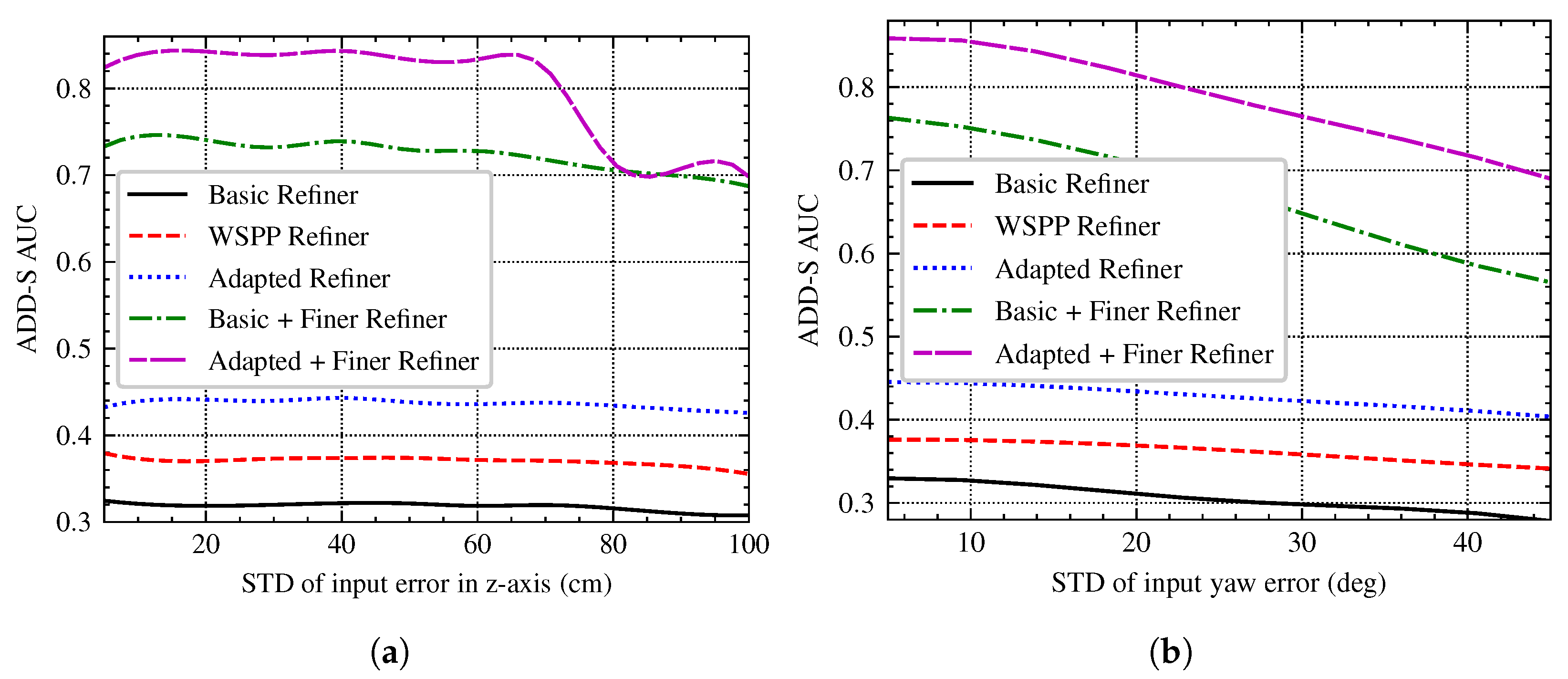
We first evaluate the effect of incorporating multi-stage refinement without any adaptation. Based on Figure 14, we can deduce the benefits of the multi-stage refiner scheme by comparing the performance of the basic + finer model with the basic baseline counterpart, where the performance improved by 147%. Additionally, we observe that even though the first part of the multi-stage pipeline (the basic refiner) was trained using less data than the WSPP refiner, the performance of the multi-stage pipeline is still better than the single-stage WSPP refiner.

This result is significant because it demonstrates that splitting the training process into two refiners can be beneficial, even when the coarse refiner is trained on a smaller dataset. In other words, training a coarse refiner on limited data, combined with a finer refiner trained on more data but over a narrow noise domain, leads to better results compared to using a larger dataset and a broader noise domain. This can be interpreted as a form of a “mixture of experts”, where each refiner specializes in different aspects of the task. Additionally, this stems from the fact that the performance gain from adding another refiner is much greater than the gain obtained by only adding new data.

Next, we examine the performance improvements achieved by combining both adaptation and multi-stage refinement. Figure 15 illustrates the performance of the multi-stage refinement pipeline composed of an adapted refiner followed by a finer refiner compared to all other models implemented in this study. When comparing the adapted + finer refiner with the adapted refiner alone, the former outperforms the latter by approximately 59–81%, depending on the input noise level, when considering the ADD-S AUC score. Additionally, we observe that the combination of the adapted and finer refiners not only outperforms both the single-stage adapted and WSPP refiners but also surpasses the multi-stage basic + finer refiner (multi-stage with non-adapted data) by approximately 10%. This demonstrates the benefits of combining domain adaptation and multi-stage refinement in the proposed multi-stage domain-adapted pose estimation framework. These findings clearly show that the proposed multi-stage domain-adapted estimation framework outperforms the classic synthetic data approach with one refiner.

5.3. In-Depth Analysis of the Proposed Multi-Stage Domain-Adapted 6D Pose Estimation Approach

Finally, we conduct a thorough and in-depth analysis of the performance of the proposed multi-stage domain-adapted 6D pose estimation approach against the experiments in Section 4.3. For this analysis, Figure 16 shows the ADD-S AUC performance under varying input depth and yaw rotation noises, at each of the four pose-refining iterations along with analyzing the MAE performance under the same conditions but after the fourth (final) refining iteration for the predicted pose estimates. This detailed examination offers valuable insights into how the integration of domain adaptation with multi-stage pose estimation in the proposed framework can improve overall system performance and resilience, particularly in the complex environment of a warehouse setting.

Figure 16a demonstrates the ADD-S AUC performance of the proposed multi-stage domain-adapted pose estimation approach against varying levels of input depth noise at each of the four pose refinement iterations applied to the predicted pose estimates generated by this pipeline. When varying the standard deviation of depth input noise, the proposed pipeline showed consistent high performance, as the ADD-S AUC score varies around 0.84 until the 70 cm standard deviation point, where it drops and varies around 0.70. Interestingly, this figure also shows continuous enhancement in the results after every pose refinement iteration. Figure 16b illustrates the MAE performance in all translational axes at the fourth (final) pose refinement iteration when the standard deviation of the input depth noise is varied. The z-axis MAE varies below 7 cm. The y-axis MAE varies around 2.5 cm, and the x-axis MAE varies around 0.5 cm. The MAE starts increasing after the 70 cm standard deviation point. This means that when 95% of the noise is within ±137 cm, the pipeline can still perform reasonably well. An important finding is the fact that the greatest relative impact was for the second network iteration (16% on the 20 STD mark). Even though the enhancement was smaller for the third iteration (4.4% on the 20 STD mark), it was significant enough. As for the fourth iteration, the enhancement started to be less pronounce (1.8% on the 20 STD mark), which justifies choosing it as the final iteration step, as any further iteration would only have marginal improvements. As expected, it was easier to estimate the $x,y$ components of the translation, while for the z component, it was more challenging, even at lower depth noise. This further justifies the choice of experimental design in Section 4.3.

Figure 16c demonstrates the detailed ADD-S AUC performance of the proposed multi-stage domain-adapted pose estimation approach against varying levels of input yaw rotation noise at each of the four pose refinement iterations applied to the predicted pose estimates generated by this pipeline. The ADD-S AUC starts from approximately 0.86 at low yaw rotational noise and progressively drops to 0.70 at 45 degrees of the standard deviation of yaw rotational noise, as displayed in Figure 16c. Similar to the first experiment, the estimation results are enhanced after every iteration. The 10 STD mark showed 17%, 3.7%, and 1.9% enhancements for the second, third, and fourth iterations, respectively. Figure 16d illustrates the MAE performance in rotational axes at the fourth (final) pose refinement iteration when the standard deviation of the input yaw rotation noise is varied. In this figure, the MAE for all axes starts at less than 3 degrees and increases as the yaw rotational noise’s standard deviation increases. When the standard deviation of the yaw input noise reaches 10, the MAE in all rotation axes was under 3 degrees, while it was less than 4.5 degrees at the same standard deviation but with a yaw input noise point of 20. In the case of estimating roll, pitch, and yaw angles, at lower noise, it is seen that the roll angle was more difficult to predict than the yaw angle. Additionally, it is seen that with increased noise in the yaw angle, all rotation estimates are impacted, which is expected due to the topology of the SO(3) group, where axes are coupled unlike the disentangled Euclidean space.

Figure 17 shows a sample of the refinement visualization results obtained with the proposed multi-stage domain-adapted pose refinement pipeline. The ground-truth pose is shown in the first image. The initial noisy pose estimate is shown in the middle image, and the refined pose is shown in the third image.

5.4. Computation Time and Efficiency

The experiments were conducted using a single NVIDIA Quadro RTX 6000 GPU and an Intel Xeon Gold 6138 processor. All training procedures utilized the PyTorch library version 2.9.0 and were based on modified versions of the official repositories for both CosyPose and CUT. For both models, we employed the Adam optimizer [37].

For training CosyPose, the following hyperparameters were used: a learning rate of $3\times {10}^{-4}$, gradient clipping set to $0.5$, and 2600 points for loss calculation. In the case of CUT, we set the learning rate to $3\times {10}^{-4}$ and applied a learning rate decay factor of $0.9$.

For the case of multi-stage refinement, where the first stage involves two iterations and the second stage consists of four iterations, the total inference time is 570 ms (compared to 440 ms of the original CosyPose model [26]), making this approach well suited for real-time applications. The inference time required for CUT (Contrastive Unsupervised Training) is 240 ms. However, this does not affect the real-time performance of the proposed approach, as CUT can be computed offline before training the pose estimator. We note that our domain adaptation network requires approximately 56 GFLOPs, while our refiner module necessitates about $1.8$ GFLOPs per iteration.

Our results demonstrate the superior performance of the proposed multi-stage domain-adapted pose estimation framework compared to the state-of-the-art single-stage pose refinement pipeline using a CosyPose network as the backbone for pose estimation. In addition to the excellent performance of this network compared to other pose estimation networks [32], the selection of this network for the proposed multi-stage pose refinement framework was an excellent choice since it can be used as both a pose initializer and for iterative-based pose refinement. Unlike other networks that require depth information during training or those based on direct estimation rules (GDR-Net, SO-Pose, and Gen6D) [32], the proposed multi-stage domain-adapted framework utilizes depth-free training information and can be evaluated with any RGB-based depth-free iterative pose refinement network. Future efforts may include a comprehensive evaluation of the proposed approach using combinations of different RGB-based iterative pose refinement networks and different types of domain adaptation networks to analyze the trade-off between different inference times and achievable performance from a real-time point of view.

Despite the promising results of this study, there are some limitations in the developed framework that could be addressed in future work. Although the use of Image-to-Image Translation as a preprocessing step makes the pipeline modular and flexible, the domain adaptation network still uses self-supervision without exploiting the available 6D pose annotations. Additionally, the current approach decreases the overall required training time, but it still requires training two models, including two backbones. This greatly increases the number of trainable parameters.

The results of this study contribute to ongoing research efforts focused on warehouse automation in smart factories. Although the proposed framework was evaluated on single-warehouse data, the self-supervision scheme employed in domain adaptation makes this framework easily extendable to other warehouse environments, especially because the proposed framework is designed using typical standard Euro pallets, facilitating knowledge transfer to similar environments. Although this shift towards fully automated warehouses and fully autonomous load carriers in smart factories might have negative effects on manual warehouse operator and driver jobs, it will create new job opportunities in sustainable engineering, artificial intelligence, and data analysis. In addition, this transition will open new avenues for human–robot collaboration to improve safety and efficiency in industrial environments, helping industries and warehouses meet environmental regulations.

6. Conclusions and Future Work

A multi-stage domain-adapted 6D pose estimation framework was developed, featuring a CUT domain adaptation network and two sequential CosyPose refiners. The first refiner is trained on high-noise data from both synthetic and domain-adapted sources, while the second refiner is trained on low-noise, domain-randomized synthetic data. This dual-refiner strategy effectively addresses varying noise levels, optimizing both training dataset size and computational efficiency. In particular, the integration of domain-adapted data further enhances the overall performance of the pipeline.

Domain adaptation using Image-to-Image Translation (CUT) was shown to significantly improve results over conventional domain-randomized, non-adapted synthetic data. The proposed multi-stage domain-adapted refinement pipeline achieved a 59–80% improvement in the ADD-S AUC metric compared to a single-stage, non-adapted baseline. Importantly, the framework is architecture-agnostic and modular, allowing application to a range of pose refinement networks. Training relies exclusively on synthetic RGB images, yet the framework demonstrated robust performance across diverse depth and rotational variations.

Future work will investigate the feasibility of sharing backbone architectures between the two refiners in the multi-stage pipeline, potentially reducing redundancy and improving efficiency. Additionally, we plan to develop an end-to-end domain adaptation and refinement pipeline that leverages supervised annotations to augment self-supervised learning within the domain adaptation network.

References

1. Fragapane, G.; Ivanov, D.; Peron, M.; Sgarbossa, F.; Strandhagen, J.O. Increasing flexibility and productivity in Industry 4.0 production networks with autonomous mobile robots and smart intralogistics. Ann. Oper. Res. 2020, 308, 125–143. [Google Scholar] [CrossRef]
2. Bechtsis, D.; Tsolakis, N. Trends in Industrial Informatics and Supply Chain Management. Int. J. New Technol. Res. 2018, 4, 91–93. [Google Scholar] [CrossRef]
3. Kedilioglu, O.; Lieret, M.; Schottenhamml, J.; Würfl, T.; Blank, A.; Maier, A.; Franke, J. RGB-D-based human detection and segmentation for mobile robot navigation in industrial environments. VISIGRAPP 2021, 4, 219–226. [Google Scholar]
4. Mok, C.; Baek, I.; Cho, Y.; Kim, Y.; Kim, S. Pallet recognition with multi-task learning for automated guided vehicles. Appl. Sci. 2021, 11, 11808. [Google Scholar] [CrossRef]
5. Tremblay, J.; Prakash, A.; Acuna, D.; Brophy, M.; Jampani, V.; Anil, C.; To, T.; Cameracci, E.; Boochoon, S.; Birchfield, S. Training deep networks with synthetic data: Bridging the reality gap by domain randomization. In Proceedings of the IEEE Conference on Computer Vision and Pattern Recognition Workshops 2018, Salt Lake City, UT, USA, 18–22 June 2018; pp. 969–977. [Google Scholar]
6. Tobin, J.; Fong, R.; Ray, A.; Schneider, J.; Zaremba, W.; Abbeel, P. Domain randomization for transferring deep neural networks from simulation to the real world. In Proceedings of the 2017 IEEE/RSJ International Conference on Intelligent Robots and Systems (IROS), Vancouver, BC, Canada, 24–28 September 2017; IEEE: Piscataway, NJ, USA, 2017; pp. 23–30. [Google Scholar]
7. Tremblay, J.; To, T.; Sundaralingam, B.; Xiang, Y.; Fox, D.; Birchfield, S. Deep object pose estimation for semantic robotic grasping of household objects. arXiv 2018, arXiv:1809.10790. [Google Scholar] [CrossRef]
8. Zhu, J.Y.; Park, T.; Isola, P.; Efros, A.A. Unpaired image-to-image translation using cycle-consistent adversarial networks. In Proceedings of the IEEE International Conference on Computer Vision 2017, Venice, Italy, 22–29 October 2017; pp. 2223–2232. [Google Scholar]
9. Hoffman, J.; Tzeng, E.; Park, T.; Zhu, J.Y.; Isola, P.; Saenko, K.; Efros, A.; Darrell, T. Cycada: Cycle-consistent adversarial domain adaptation. In Proceedings of the International Conference on Machine Learning 2018, Stockholm, Sweden, 10–15 July 2018; pp. 1989–1998. [Google Scholar]
10. Park, T.; Efros, A.A.; Zhang, R.; Zhu, J.Y. Contrastive Learning for Unpaired Image-to-Image Translation. In Proceedings of the European Conference on Computer Vision 2020, Virtual, 23–28 August 2020. [Google Scholar]
11. Zou, S.; Huang, Y.; Yi, R.; Zhu, C.; Xu, K. CycleDiff: Cycle Diffusion Models for Unpaired Image-to-image Translation. arXiv 2025, arXiv:2508.06625. [Google Scholar]
12. Su, X.; Song, J.; Meng, C.; Ermon, S. Dual diffusion implicit bridges for image-to-image translation. arXiv 2022, arXiv:2203.08382. [Google Scholar]
13. Parmar, G.; Park, T.; Narasimhan, S.; Zhu, J.Y. One-step image translation with text-to-image models. arXiv 2024, arXiv:2403.12036. [Google Scholar]
14. Liu, Y.; Li, S.; Lin, Z.; Wang, F.; Liu, S. CycleVAR: Repurposing Autoregressive Model for Unsupervised One-Step Image Translation. arXiv 2025, arXiv:2506.23347. [Google Scholar]
15. Hinterstoisser, S.; Cagniart, C.; Ilic, S.; Sturm, P.; Navab, N.; Fua, P.; Lepetit, V. Gradient response maps for real-time detection of textureless objects. IEEE Trans. Pattern Anal. Mach. Intell. 2011, 34, 876–888. [Google Scholar] [CrossRef] [PubMed]
16. Collet, A.; Martinez, M.; Srinivasa, S.S. The MOPED framework: Object recognition and pose estimation for manipulation. Int. J. Robot. Res. 2011, 30, 1284–1306. [Google Scholar] [CrossRef]
17. Xiang, Y.; Schmidt, T.; Narayanan, V.; Fox, D. Posecnn: A convolutional neural network for 6d object pose estimation in cluttered scenes. arXiv 2017, arXiv:1711.00199. [Google Scholar]
18. Lepetit, V.; Moreno-Noguer, F.; Fua, P. Epnp: An accurate o (n) solution to the pnp problem. Int. J. Comput. Vis. 2009, 81, 155. [Google Scholar] [CrossRef]
19. Peng, S.; Liu, Y.; Huang, Q.; Zhou, X.; Bao, H. Pvnet: Pixel-wise voting network for 6dof pose estimation. In Proceedings of the IEEE/CVF Conference on Computer Vision and Pattern Recognition 2019, Long Beach, CA, USA, 16–20 June 2019; pp. 4561–4570. [Google Scholar]
20. Fischler, M.A.; Bolles, R.C. Random sample consensus: A paradigm for model fitting with applications to image analysis and automated cartography. Commun. ACM 1981, 24, 381–395. [Google Scholar] [CrossRef]
21. Hodaň, T.; Sundermeyer, M.; Drost, B.; Labbé, Y.; Brachmann, E.; Michel, F.; Rother, C.; Matas, J. BOP challenge 2020 on 6D object localization. In Proceedings of the European Conference on Computer Vision 2020, Virtual, 23–28 August 2020; Springer: Berlin/Heidelberg, Germany, 2020; pp. 577–594. [Google Scholar]
22. Song, C.; Song, J.; Huang, Q. Hybridpose: 6d object pose estimation under hybrid representations. In Proceedings of the IEEE/CVF Conference on Computer Vision and Pattern Recognition 2020, Virtual, 13–19 June 2020; pp. 431–440. [Google Scholar]
23. Tekin, B.; Sinha, S.N.; Fua, P. Real-time seamless single shot 6d object pose prediction. In Proceedings of the IEEE Conference on Computer Vision and Pattern Recognition 2018, Salt Lake City, UT, USA, 18–22 June 2018; pp. 292–301. [Google Scholar]
24. Hu, Y.; Fua, P.; Wang, W.; Salzmann, M. Single-stage 6d object pose estimation. In Proceedings of the IEEE/CVF Conference on Computer Vision and Pattern Recognition 2020, Virtual, 13–19 June 2020; pp. 2930–2939. [Google Scholar]
25. Li, Y.; Wang, G.; Ji, X.; Xiang, Y.; Fox, D. Deepim: Deep iterative matching for 6d pose estimation. In Proceedings of the European Conference on Computer Vision (ECCV) 2018, Munich, Germany, 8–14 September 2018; pp. 683–698. [Google Scholar]
26. Labbé, Y.; Carpentier, J.; Aubry, M.; Sivic, J. CosyPose: Consistent multi-view multi-object 6D pose estimation. arXiv 2020, arXiv:2008.08465. [Google Scholar]
27. Hai, Y.; Song, R.; Li, J.; Hu, Y. Shape-constraint recurrent flow for 6d object pose estimation. In Proceedings of the IEEE/CVF Conference on Computer Vision and Pattern Recognition 2023, Vancouver, BC, Canada, 18–22 June 2023; pp. 4831–4840. [Google Scholar]
28. Xu, Y.; Lin, K.Y.; Zhang, G.; Wang, X.; Li, H. Rnnpose: 6-dof object pose estimation via recurrent correspondence field estimation and pose optimization. IEEE Trans. Pattern Anal. Mach. Intell. 2024, 46, 4669–4683. [Google Scholar] [CrossRef] [PubMed]
29. Li, F.; Vutukur, S.R.; Yu, H.; Shugurov, I.; Busam, B.; Yang, S.; Ilic, S. Nerf-pose: A first-reconstruct-then-regress approach for weakly-supervised 6d object pose estimation. In Proceedings of the IEEE/CVF International Conference on Computer Vision 2023, Vancouver, BC, Canada, 18–22 June 2023; pp. 2123–2133. [Google Scholar]
30. Haugaard, R.L.; Buch, A.G. Surfemb: Dense and continuous correspondence distributions for object pose estimation with learnt surface embeddings. In Proceedings of the IEEE/CVF Conference on Computer Vision and Pattern Recognition 2022, New Orleans, LA, USA, 19–24 June 2022; pp. 6749–6758. [Google Scholar]
31. Li, Y.; Mao, Y.; Bala, R.; Hadap, S. Mrc-net: 6-dof pose estimation with multiscale residual correlation. In Proceedings of the IEEE/CVF Conference on Computer Vision and Pattern Recognition 2024, Seattle, WA, USA, 17–21 June 2024; pp. 10476–10486. [Google Scholar]
32. Liu, J.; Sun, W.; Yang, H.; Zeng, Z.; Liu, C.; Zheng, J.; Liu, X.; Rahmani, H.; Sebe, N.; Mian, A. Deep learning-based object pose estimation: A comprehensive survey. arXiv 2024, arXiv:2405.07801. [Google Scholar] [CrossRef]
33. Rennie, C.; Shome, R.; Bekris, K.E.; De Souza, A.F. A dataset for improved rgbd-based object detection and pose estimation for warehouse pick-and-place. IEEE Robot. Autom. Lett. 2016, 1, 1179–1185. [Google Scholar] [CrossRef]
34. Epic Games. Unreal Engine; Epic Games, Inc.: Cary, NC, USA, 2019. [Google Scholar]
35. Hinterstoisser, S.; Lepetit, V.; Ilic, S.; Holzer, S.; Bradski, G.; Konolige, K.; Navab, N. Model based training, detection and pose estimation of texture-less 3d objects in heavily cluttered scenes. In Proceedings of the Asian Conference on Computer Vision 2012, Daejeon, Korea, 5–9 November 2012; Springer: Berlin/Heidelberg, Germany, 2012; pp. 548–562. [Google Scholar]
36. Liu, X.; Iwase, S.; Kitani, K.M. Stereobj-1m: Large-scale stereo image dataset for 6d object pose estimation. In Proceedings of the IEEE/CVF International Conference on Computer Vision 2021, Virtual, 11–17 October 2021; pp. 10870–10879. [Google Scholar]
37. Kingma, D.P.; Ba, J. Adam: A method for stochastic optimization. arXiv 2014, arXiv:1412.6980. [Google Scholar]
Figure 1. Six-dimensional pose of a pallet relative to the camera frame.
Machines 13 01126 g001
Figure 2. (a) Real warehouse data image. (b) Synthetic warehouse data image. The simulated synthetic data is generated using computer simulations but does not appear realistic, resulting in a domain gap between the real and synthetic domains.
Machines 13 01126 g002
Figure 3. Two examples (a,b) of domain-randomized images. Pallets are rendered with randomized backgrounds, lighting conditions, and materials.
Machines 13 01126 g003
Figure 4. Samples from the RPP dataset.
Machines 13 01126 g004
Figure 5. Samples from the WSPP dataset.
Machines 13 01126 g005
Figure 6. Samples from the RSPP dataset.
Machines 13 01126 g006
Figure 7. A flowchart for the proposed multi-stage domain-adapted pose estimation framework.
Machines 13 01126 g007
Figure 8. Training CUT to adapt WSPP data.
Machines 13 01126 g008
Figure 9. Samples from the adapted-WSPP dataset.
Machines 13 01126 g009
Figure 10. Noise sampling for refiner network training. The refiner is trained using labeled synthetic data by inputting the ground-truth pose with additive noise sampled from a normal distribution ( ε N ( M e a n , S T D ) ).
Machines 13 01126 g010
Figure 11. Training scenarios for the single-stage refinement pipeline: (a) basic refiner, (b) WSPP refiner, (c) adapted refiner.
Machines 13 01126 g011
Figure 12. Training scenarios for the single-stage refinement pipeline: (a) the basic refiner with a finer refiner pipeline and (b) the adapted refiner with a finer refiner pipeline.
Machines 13 01126 g012
Figure 13. Performance comparison for the scenarios of the single-stage refinement pipeline against the experiments in Section 4.3. The basic, WSPP, and adapter refiners are evaluated on RPP data (a) under varying levels of yaw rotation noise and (b) under varying levels of depth noise. Both plots showcase noticeable and consistent performance gains when using the CUT UNIT network as the domain adaptation technique.
Machines 13 01126 g013
Figure 14. Performance comparison between the multi-stage and single-stage refinement pipelines without domain adaptation against the experiments in Section 4.3. The basic, WSPP, and basic + finer refiners are evaluated on RPP data (a) under varying levels of depth noise and (b) under varying levels of yaw rotation noise. Both plots showcase noticeable and consistent performance gains when using the multi-stage approach even before domain adaptation.
Machines 13 01126 g014
Figure 15. Performance comparison between all refinement pipelines developed in this study against the experiments in Section 4.3. All models were evaluated on RPP data (a) under varying levels of depth noise and (b) under varying levels of yaw rotation noise. The proposed multi-stage domain-adapted approach demonstrates the best performance results among all other developed models.
Machines 13 01126 g015
Figure 16. Performance analysis of the proposed multi-stage domain-adapted pose estimation approach against the experiments in Section 4.3, evaluated on RPP data. (a) ADD-S AUC performance under varying levels of input depth noise at each of the four pose refinement iterations. (b) MAE at the fourth pose refinement iteration under varying levels of input depth noise. (c) ADD-S AUC performance under varying levels of input yaw rotation noise at each of the four pose refinement iterations. (d) MAE at the fourth pose refinement iteration under varying levels of input yaw rotation noise.
Machines 13 01126 g016
Figure 17. Visualization of the ground-truth, initial, and refined poses: Using the given pose (ground-truth, initial estimate, or refined pose), the CAD model is projected to the image plane, producing a rendered image of the pose. Then, the real RGB image is overlayed by the rendered image, providing a visualization of how well the pose corresponds to the true pose. The rendered pallet is visualized using a dark shade. (a) The rendered ground-truth pose matches the RGB image perfectly. (b) The rendered initial pose does not match the RGB image. (c) The rendered refined pose looks almost identical to the ground truth.
Machines 13 01126 g017