Article

Improved FMEA Risk Assessment Based on Load Sharing and Its Application to a Magnetic Lifting System

College of Mechanical and Vehicle Engineering, Changchun University, 6543 Satellite Road, Changchun 130022, China
*
Author to whom correspondence should be addressed.
Machines 2025, 13(12), 1113; https://doi.org/10.3390/machines13121113
Submission received: 29 October 2025 / Revised: 20 November 2025 / Accepted: 28 November 2025 / Published: 2 December 2025
(This article belongs to the Section Advanced Manufacturing)

Abstract

Failure Mode and Effects Analysis (FMEA) is a systematic risk assessment tool that effectively evaluates the safety and reliability of products prior to their deployment. However, traditional FMEA fails to consider and leverage inherent system-specific information during risk assessment, while also neglecting the weights of risk factors (RFs) when processing data related to the Risk Priority Number (RPN). This leads to significant subjectivity in the final risk ranking of failure modes. To overcome these drawbacks, this study proposes an improved FMEA risk assessment method based on load sharing, aiming to develop an improved FMEA method that addresses the critical limitations of traditional approaches by integrating load sharing principles and systematic weight determination, thereby enhancing risk assessment objectivity and accuracy in complex multi-component systems. First, probabilistic linguistic terms are adopted to quantify experts’ risk assessment information, and the geometric mean method is then used to aggregate assessments from multiple experts. Second, the Fuzzy Best–Worst Method (FBWM) is employed to determine the relative weights of the three RPN factors (Occurrence, Severity, and Detection). Additionally, partial system structural data are obtained through load sharing, and these data—combined with the calculated factor weights—are integrated into the Technique for Order Preference by Similarity to Ideal Solution (TOPSIS) to generate the final risk ranking of failure modes. Finally, a case study of a magnetic crane is conducted to verify the feasibility and effectiveness of the proposed method, supplemented by comparative experiments to demonstrate its superiority.

1. Introduction

Failure Mode and Effects Analysis (FMEA) [1,2] is a systematic analysis method widely used in the field of reliability engineering. The calculation process of traditional FMEA consists of three steps. First, experts conduct risk rating on the Severity (S), Occurrence (O), and Detection (D) among the risk factors (RFs) of product failure modes to obtain the RF values for all failure modes. Second, the S, O, and D values of each failure mode are multiplied respectively to obtain the Risk Priority Number (RPN) for that failure mode. Finally, ranking is performed based on the RPN values of each failure mode, resulting in the risk ranking of failure modes. This method conducts quantitative ranking of various risks. By prioritizing the handling of high-risk failure items and guiding teams to develop targeted preventive measures, it effectively avoids the occurrence of failures and enhances the reliability of systems and products. However, traditional FMEA [3] is highly subjective and has several limitations [4] in practical applications: (1) simple rating fails to convey experts’ subjective information; (2) it treats the weights of RFs as equal; (3) the RPN calculation is simplistic, leading to unreliable rankings; (4) the entire process fails to consider certain inherent information of the system itself.
Traditional FMEA typically uses numerical values from one to nine to represent risk levels, where a higher value indicates greater risk. However, such a simplistic rating system fails to capture experts’ nuanced judgments. To address this issue, many scholars have introduced the concept of fuzziness. For instance, Tian et al. [5] proposed an interval number-based FMEA method for the risk assessment of electric vehicle charging piles, which effectively addressed the fuzziness of expert judgments by quantifying risk values into intervals. Their results indicated that the method could accurately identify high-risk failure modes such as charging interface overheating. Another example is Li [6], who successfully quantified the fuzziness and reliability of expert evaluations by integrating Z-numbers, accurately identifying high-risk failure modes in crane operations (e.g., hydraulic system leakage and brake system wear). Both approaches struggle to represent situations where experts simultaneously assign probabilities to multiple linguistic terms. While this limitation can lead to a notable information loss, Pang et al. [7] demonstrated that Probabilistic Linguistic Term Sets are specifically designed to preserve this information in FMEA contexts.
To resolve this, some scholars have introduced Linguistic Term Sets (LTSs) [8], such as Probabilistic Linguistic Term Sets (PLTSs) [9], Double Hierarchy Linguistic Term Sets [10], and Probabilistic Hesitant Fuzzy Linguistic Term Sets [11]. All of these approaches integrate LTSs with probability theory. Specifically, LTSs can accurately depict the risk levels in FMEA, while probability effectively quantifies the credibility of experts’ judgments on these levels. Compared with interval-number-based methods, this LTS–probability combination conveys richer evaluation information. In contrast to Z-numbers, it is not only simpler, more intuitive, and easier to compute but also more user-friendly for experts, thereby reducing the evaluation threshold. In the FMEA calculation process, the weights of S, O, and D are usually treated as equal, which is irrational. As a result, numerous studies have focused on calculating the weights of S, O, and D in FMEA. For example, some methods rely on experts to directly assign weights, but this approach may lead to significant discrepancies in expert opinions. To mitigate this, scholars have introduced Multi-Criteria Decision Making (MCDM) [12] to calculate these weights. María et al., for instance, proposed an FMEA method based on the Analytic Hierarchy Process (AHP) [13,14], which computes weights by constructing a comparison matrix. Another example is İrem et al., who used the Best–Worst Method (BWM) [15,16]. They first identified the best and worst criteria to generate comparison data, and then calculated weights by solving a system of inequalities. Both BWM and AHP can reduce the subjectivity of risk assessment results. Compared with AHP, BWM requires fewer pairwise comparisons, thus reducing subjectivity more effectively. This study will adopt a method that combines LTS–probability integration with BWM to achieve the quantification of risk assessment and the calculation of RF weights.
With the development of combinations of FMEA and MCDM [17,18,19], methods that integrate multiple MCDMs have emerged. In FMEA-MCDM combinations, experts typically provide data in two tables: one contains data on the mutual comparisons of S, O, and D, and the other includes data on S, O, and D for each failure mode of the system. Typically, subjective weighting methods such as AHP and BWM are used to calculate subjective weights based on the former set of data. Then, objective weighting methods like the entropy weight method and Criteria Importance Through Inter-criteria Correlation (CRITIC) [20] are applied to compute objective weights using the latter set of data. Finally, parameters are used to adjust the proportion of subjective and objective weights, resulting in the final comprehensive weights. For example, Wang et al. [11] developed and successfully applied an integrated weighting methodology combining the Best–Worst Method (BWM) and Multi-Dimensional Decision Making (MDM) to determine the weights of risk factors (RFs) for machine tools. Their research demonstrated that this comprehensive weighting approach not only effectively reduced the sensitivity of risk prioritization outcomes but also significantly mitigated the influence of subjective judgments on the evaluation process. However, both single weighting methods and comprehensive weight algorithms are based on experts’ subjective evaluations and lack support from real-world conditions. This highlights a more fundamental limitation: the risk assessment process remains decoupled from the physical architecture of the system. Expert judgments, though valuable, cannot precisely quantify the physical dependencies between components and the effects of failure propagation. This disconnect can lead to risk prioritization that deviates from the true reliability profile of the system. Therefore, we propose an FMEA method based on load sharing, which obtains certain structural data by analyzing the structure of the research object to reduce the subjectivity of FMEA.
Load sharing [21,22] refers to the phenomenon in multi-component systems where components may interact with each other in different proportions during operation. When a component fails, its load is borne by adjacent components, which increases the likelihood of failure for those adjacent components. Specifically, the greater the load, the higher the probability of failure. In systems with both series and parallel connections, the severity of series connections is far greater than that of parallel connections. For series-connected components, the failure of any single component will lead to the failure of the entire system. In contrast, for parallel-connected components, the failure of one parallel component will result in the load being shared by other parallel components, and will not cause the entire system to fail. Therefore, this study is theoretically motivated by the integration of the load sharing model into the FMEA framework. The core rationale is to incorporate objective system structural information into risk assessment, creating a subjective–objective fusion. This allows for the quantification of failure propagation and system-level impact, shifting the focus from the “likelihood of component failure” to the “conditional probability of component failure causing system failure.” A component with a high O value might pose a low actual risk if it is surrounded by sufficient redundancy (parallel structure), whereas a component with a moderate O value but located in a critical serial path might have its risk severely underestimated. This approach fundamentally differs from existing MCDM-FMEA methods by introducing inherent, objective information dictated by the physical system structure, ensuring the final risk ranking reflects not only what the risk experts “perceive” but also what the risk the system structure “reveals”.
In FMEA risk ranking, the product calculation of O, S, and D is overly simplistic. Therefore, many scholars have introduced MCDM-based ranking methods. VlseKriterijumska Optimizacija I Kompromisno Resenje (VIKOR) [23] and Technique for Order Preference by Similarity to Ideal Solution (TOPSIS) [24,25] are two commonly used MCDM methods. The VIKOR method performs well in handling conflicting objectives, while the TOPSIS method focuses more on the proximity of alternatives to the ideal solution. These ranking methods are usually used in combination with approaches such as BWM, AHP, and comprehensive weighting methods. Typically, relative weights are first calculated via MCDM and then integrated into VIKOR or TOPSIS for ranking. This study will simultaneously integrate the data obtained from load sharing and the original data into TOPSIS to generate the final risk ranking.
The structure of this study is as follows: Section 2 presents the preliminaries of load sharing. Section 3.1 and Section 3.2 introduce the FBWM method combining LTS with probability, which is used for the quantification of experts’ risk assessments and the calculation of RF weights. Section 3.3 focuses on load sharing: by analyzing the spatial states of failure modes, the probability of each failure mode causing system failure is derived based on the O values provided by experts. Section 3.4 covers TOPSIS-based ranking: the values obtained from load sharing and the original S, O, and D values are simultaneously integrated into TOPSIS to obtain the final risk ranking. Section 4 presents a case study applying the proposed method to a magnetic lifting system, supplemented by sensitivity and comparative analyses. The paper concludes with research findings and future directions in Section 5.

2. Load Sharing Method

A load sharing system [26] is a redundant architecture composed of functionally parallel and interdependent components. Under normal operating conditions, all components in the system collectively bear the operational load. Its core characteristic is that, when one or more components fail, the system does not immediately cease to function; instead, it dynamically redistributes the load previously borne by the failed components to the remaining operational ones.
We consider the spatial arrangement relationship of each component, where θ i j represents the connection relationship between the non-faulty component i and the faulty component j. θ i j = 1 indicates a connection exists and θ i j = 0 indicates no connection. Here, i = 1 , 2 , , n ; j = 1 , 2 , , n , with n being the total number of components.
θ 11 θ 12 θ 1 n θ 21 θ 22 θ 2 n θ n 1 θ n 2 θ n n
To distribute the load of a faulty component proportionally among each non-faulty component, a normalization process is performed on each column, as shown in Formula (2). Finally, we obtain a matrix V, where v i j represents the load proportion of each faulty component relative to the surrounding components.
v i j = θ i j i = 1 n θ i j
V = v 11 v 12 v 1 n v 21 v 22 v 2 n v n 1 v n 2 v n n
The number of spatial neighbors of a component is determined by the number of its connections to other components. The total load L of the system is shared by all components, which are allocated the total load L in the proportion of r 1 , r 2 , r n . The system fails when the total load borne by the non-faulty components is less than the total load L. z i denotes the initial load of the i-th component.
z i = r i L i = 1 n r i
Define z i ( j ) as the load of component i when the faulty component j fails; the formula is shown in Formula (5).
z i ( j ) = z i + v i j z j
If component k, which is adjacent to component i, also fails when the faulty component j is in a failed state, the situation is as shown in Formula (6).
z i ( j , k ) = z i ( j ) + v i k z k = z i + v i j z j + v i k z k
The system fails when the total load of the working components is less than the total load applied to the system, i.e., i = 1 n z i < L .
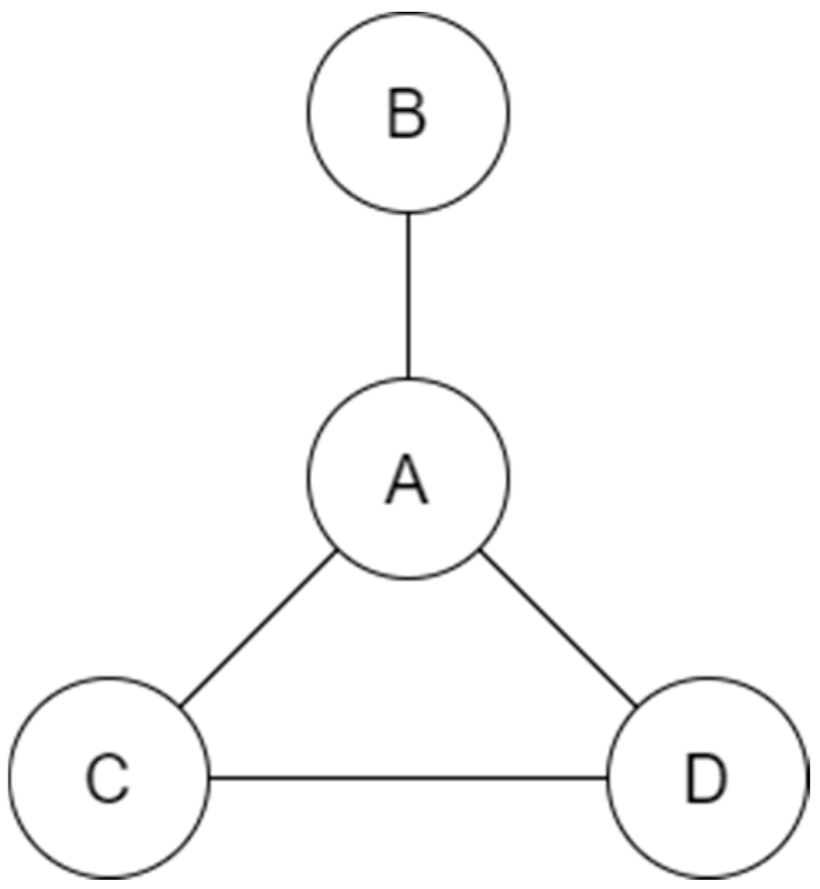
To explain under what circumstances the system fails, let us consider a four-component parallel gear system, as shown in Figure 1. Component systems A and B are connected by a shaft, while component systems C and D are connected by another shaft. When component system A fails, its load is entirely transferred to component system B; systems C and D remain unaffected. However, if gear system B also fails after the failure of gear system A, the combined load of both A and B cannot be transferred to any other component, causing the entire system to halt.
In summary, the core value of the load sharing model lies in its ability to translate the physical topology of a system—the connectivity between components into dynamic, quantifiable reliability parameters. By simulating failure propagation paths and load redistribution processes, it reveals how local failures can evolve into system-level failures through intrinsic systemic interdependencies. This model provides the theoretical basis and a computational framework for assessing the system-level impact of component failures. Thereby, it incorporates the often-overlooked characteristics of system architecture into traditional reliability analysis, laying a solid foundation for its subsequent integration with the FMEA methodology to conduct more comprehensive risk assessments.

3. Methodology

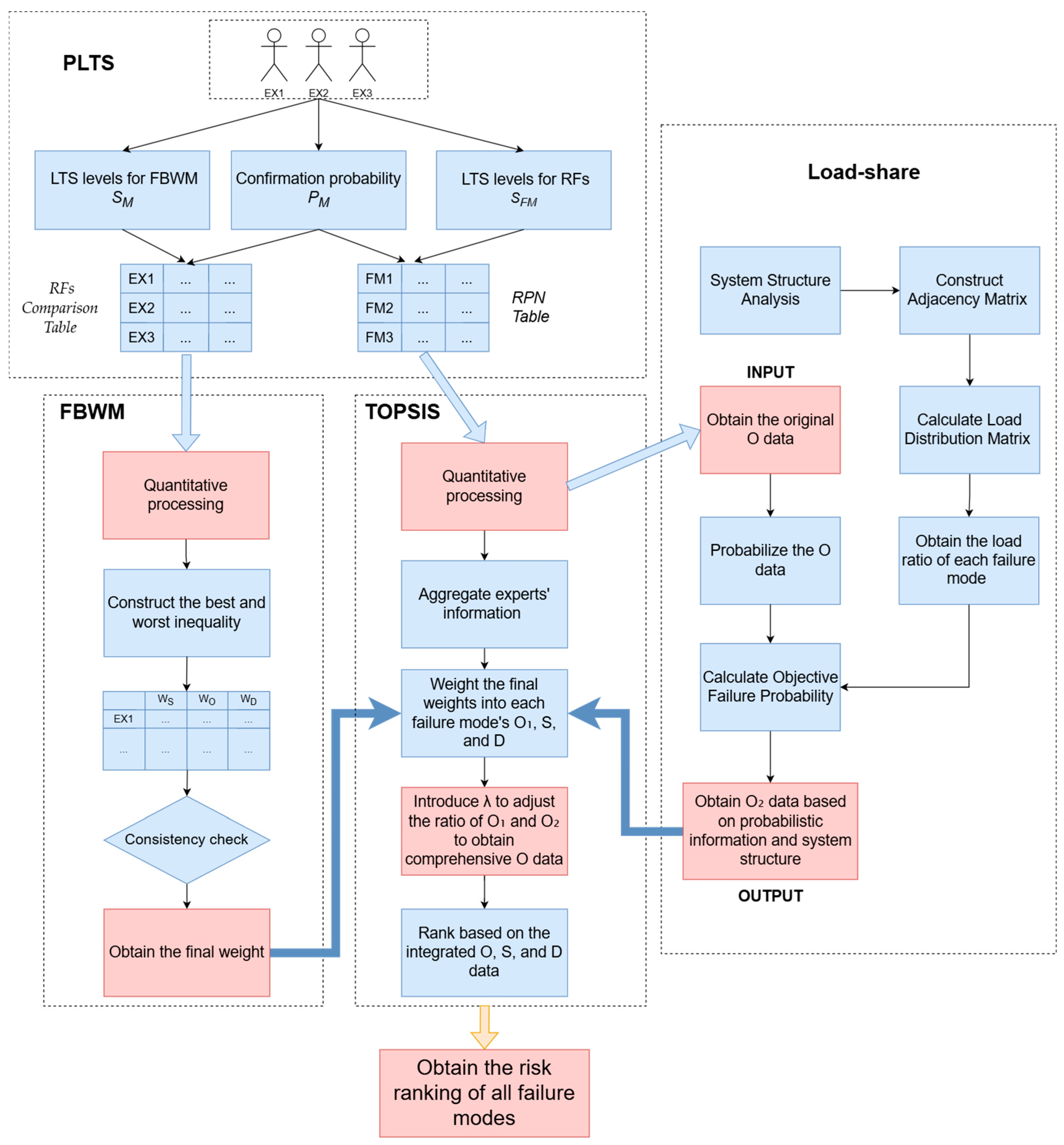
The method proposed in this paper is mainly divided into four parts. The first part is the PLTS method constructed by LTS and probability, which is used to quantify expert evaluation information. The second part is FBWM, which is applied to calculate the weights of RFs. The third part is load sharing, which deduces the probability of system failure caused by the occurrence of all fault modes based on the evaluation information of O. The fourth part is TOPSIS, which integrates the derived data into the original data for risk ranking, as specifically shown in Figure 2.

3.1. PLTS

In this section, we will define risk assessment criteria using the LTS and construct a PLTS risk assessment framework combined with probability, which is used for the collection and calculation of expert evaluation information.
Step 1: Define Risk Assessment Criteria
In the PLTS framework, two risk assessment criteria need to be defined. One is the standard S F M for all fault mode RFs provided during the risk assessment phase, and the other is the comparison standard S M for RFs provided when calculating the weights of RFs.
S F M = s 1 = A b s o l u t e l y   Low ( A L ) s 2 = V e r y   Low ( V L ) s 3 = L o w ( L ) s 4 = M oderate   Low ( M L )   s 5 = M o d e r a t e ( M ) s 6 = M oderate   High ( M H ) s 7 = H i g h ( H ) s 8 = V e r y   High ( V H ) s 9 = A b s o l u t e l y   High ( A H )
S M = m 1 = E q u a l   i m p o r t a n t ( E I ) m 2 = V e r y   w e a k   i m p o r t a n t ( V W I ) m 3 = W e a k   i m p o r t a n t ( W I ) m 4 = V e r y   moderate   i m p o r t a n t ( V M I )   m 5 = M o d e r a t e   important ( M I ) m 6 = S t r o n g   important ( S I ) m 7 = V e r y   strong   important ( V S I ) m 8 = V e r y   important ( V I ) m 9 = E x t r e m e   important ( E I )
Step 2: Define the Confirmation Probability Criterion
Specify the confirmation probability P M , which is used to verify the reliability of Criteria (7) and (8) during the experts’ risk assessment process.
P M = p 1 = A b s o l u t e l y   R e l i a b l e ( A R ) ( 0.9 ) p 2 = V e r y   H i g h l y   R e l i a b l e ( V H R ) ( 0.8 ) p 3 = H i g h l y   R e l i a b l e ( H R ) ( 0.7 ) p 4 = E q u a l l y   Reliable ( E R ) ( 0.5 ) p 5 = W e a k l y   R e l i a b l e ( W R ) ( 0.3 ) p 6 = V e r y   W e a k l y   R e l i a b l e ( V W R ) ( 0.2 ) p 7 = A b s o l u t e l y   U n r e l i a b l e ( A U ) ( 0.1 )
Step 3: Standard Form of Expert Evaluation
We ask experts to select criteria from (7) to conduct risk assessment on the RFs of fault modes and provide the corresponding confirmation probability for Criterion (9). If an expert only adopts one criterion for the RFs of a fault mode, i.e., the set S = { s i } , it can be denoted as { ( s i , p j ) } . If the expert hesitates about the k-th criterion, it can be denoted as { ( s i , p j ) , ( s k , 1 p j ) } . Therefore, the representation form of the fault mode is as shown in Formula (10).
D M = { ( s i , p j ) | i = 1 , 2 , , 9 ; j = 1 , 2 , , 6 } { ( s i , p j ) , ( s k , 1 p j ) | k = 1 , 2 9 } i f     s k S  
For example, if an expert evaluates the RFs of a certain fault mode D M 1 as s 7 and provides a confirmation probability of p 1 for s 7 , but hesitates about the criterion s 8 , the expert’s evaluation can be denoted as D M 1 = { ( s 7 , p 1 ) , ( s 8 , 1 p 1 ) } .
Step 4: Quantify Risk Assessment Information
If the risk assessment information is denoted in the form of Formula (10), the score is obtained by multiplying each LTS level by its corresponding probability and then summing the products. As shown in Formula (11), score formulae for the two scenarios are derived.
D D M = i × p j i × p j + k × ( 1 p j ) i f     s k S
Step 5: Aggregate Experts’ Risk Assessment Data
If m experts provide evaluation results as { D D M 1 , D D M 2 , , D D M m } , the aggregation formula [27] is as shown in Formula (12).
D = ( D D M 1 × D D M 2 × × D D M m ) 1 m
The PLTS framework effectively quantifies expert judgments in FMEA by combining linguistic terms with probability distributions. It preserves critical assessment information while minimizing information loss, serving as a vital input for subsequent FBWM and load sharing analyses in our integrated risk evaluation methodology.

3.2. FBWM

The BWM is a new weight calculation method proposed by Rezaei (2015) [15]. This section will describe the process of calculating weights using the Fuzzy Best–Worst Method (FBWM).
Step 1: Confirm the Decision Criteria
In this step, we will determine which criteria to calculate weights for. Assume there are n decision criteria, and these criteria form the set A = { a 1 , a 2 , , a n } .
Step 2: Identify the Best and Worst Criteria Among All Criteria
In this step, experts are required to select the best criterion a B and the worst criterion a W from set A based on the decision criteria.
Step 3: Construct Comparison Relationships
Construct two sets of comparison data, a B and a W , which are derived from comparing A B and A W with each criterion the set A, respectively.
A B = ( a B 1 , a B 2 , , a B n ) A W = ( a 1 W , a 2 W , , a n W ) T
a B 1 represents the multiple of the best criterion a B relative to criterion a 1 , and a 1 W represents the multiple of criterion a 1 relative to the worst criterion a W . Here, both a B B and a W W are equal to 1.
Step 4: Determine the Optimal Weights
In this step, we assume the final weights of the criteria are w = ( w 1 , w 2 , , w n ) , where the weights corresponding to a B and a W are w B and w W , respectively. In the comparison data, a B 1 is the value of a B / a 1 , and this value should be close to w B / w 1 . Therefore, we transform the problem into finding w, such that the maximum values of w B / w j a B j and w j / w W a j W are both less than a very small number ξ * , as shown in Formula (14).
w B w j a B j ξ * ,   j w B w j a B j ξ * ,   j j = 1 n w j = 1 w j 0
Step 5: Consistency Check
The FBWM is based on comparison data, so a consistency check is required. The consistency check formula for BWM is shown in Formula (15) [28].
C R = ξ * ξ
Here, ξ is determined by a B W . However, in a fuzzy environment, the value of a B W is a fraction, so it is calculated using Formula (16) [28].
( a B W ξ ) × ( a B W ξ ) = a B W + ξ
Typically, there are two solutions for ξ , and the smaller one is selected as the criterion. If C R 0.1 , the consistency check is passed.
This section has established the FBWM as a robust approach for determining risk factor weights in FMEA. By incorporating PLTS to address uncertainties in expert judgment, FBWM preserves the efficiency of traditional BWM while significantly enhancing its capacity to capture subjective ambiguity.

3.3. FMEA and Load Sharing

In FMEA, experts provide numerical values for the O, S, and D of failure modes to rank the failures. Typically, the weights of O, S, and D are calculated by combining them with MCDM methods, which are then integrated into the RPN table for ranking. However, both the data from MCDM and the data in the RPN table are based on experts’ subjective evaluations. Therefore, we analyze the occurrence probability (O) through experts’ opinions and, in combination with the system structure, calculate under what circumstances the failure of each component will lead to the failure of the entire system.
Step 1: Obtain the Failure Probability of Components
Experts provide the O values for each of the n failure modes in FMEA, denoted as O = { o 1 , o 2 , , o n } . Using the evaluation criteria S F M presented in Section 3.1, O is processed via Formula (17) to convert it into a probability format, where M A X ( S F M ) represents the highest index (set to 9 in this paper). This yields the occurrence probability of each mode as E = { e 1 , e 2 , , e n } .
e i = o i M A X ( S F M )
Step 2: Define the Failure Probability of the Next State
Assume that, when component j 1 , j 2 , , j n around component i fails, the load on component i will increase, and thus its probability of failure will rise, as expressed in Formula (18).
e i ( j 1 , j 2 , j n ) = ( 1 + z i ( j 1 , j 2 , j n ) L ) e i
Step 3: Probability of Component Failure
A component’s failure will lead to the failure of the entire system only when all adjacent components that can share its load have failed. Therefore, the probability of a component failure causing the entire system to fail is taken as the probability of that failure mode.
If there are n components around component i, the probability of component i failing when all surrounding components have failed is shown in Formula (18), where i is the target component and j 1 , j 2 , , j n represent the independent failure sequences of the surrounding components.
By multiplying the probabilities s of all states prior to the system failure, the final probability F i ( j 1 , j 2 , j 3 , , j n ) is obtained, as shown in Formula (19).
F i ( j 1 , j 2 , j 3 , , j n ) = e j 1 × e j 2 ( j 1 ) × e j 3 ( j 1 , j 2 ) × × e j n ( j 1 , j 2 , , j n 1 ) × e i ( j 1 , j 2 , j n )
When there are correlations between j 1 , j 2 , , j m , different failure sequences may lead to different final outcomes. Therefore, we propose a weighting calculation method to aggregate the results from different sequences, as shown in Formula (20).
F i = w 1 × F i ( j 1 , j 2 , j 3 , , j m ) + w 2 × F i ( j 2 , j 1 , j 3 , , j m ) + , + w m ! × F i ( j m , j m 1 , j m 2 , , j 1 )
Here, w 1 , w 2 , , w m ! denote the respective weight coefficients assigned to each potential sequence.
This section integrated load sharing modeling with FMEA, enhancing risk assessment by quantifying how component failures propagate through system structures. This physics-based approach complements expert judgment with objective data, improving failure mode prioritization accuracy.
The detailed derivation of the load sharing model and the calculation of weight are provided in Appendix A.

3.4. TOPSIS

TOPSIS is a well-established MCDM method [29]. Its core concept is based on the idea that the optimal alternative should have the shortest geometric distance from the positive ideal solution (PIS) and the longest geometric distance from the negative ideal solution (NIS). The PIS is a hypothetical solution that comprises the best values for all criteria, whereas the NIS consists of the worst values. TOPSIS is adopted in this study for the final risk ranking due to its intuitive logic, computational simplicity, and its ability to provide a comprehensive framework for simultaneously handling both the objective data derived from load sharing and the subjective data from expert evaluations.
Step 1: Process Subjective and Load Sharing Data
In load sharing, we obtained some structural data from FMEA. Since the data scale differs from that of S, O, and D, normalization [30] is performed in Formula (21) as follows:
b i = a i min ( a j ) max ( a j ) min ( a j ) , i = 1 , 2 , , n ; j = 1 , 2 , , n
where ( a 1 , a 2 , , a n ) denotes the data to be processed.
After standardizing all of the O-data F obtained from load sharing using Formula (21), we denote the processed data as O F * = ( O 1 * , O 2 * , , O n * ) , where n is the number of failed components.
There are m experts evaluate the S, O, and D of the failed components, yielding respective evaluations S i = ( s 1 i , s 2 i , , s n i ) , O i = ( o 1 i , o 2 i , , o n i ) , and D i = ( d 1 i , d 2 i , , d n i ) . All experts’ S, O, and D data are standardized via Formula (21) to obtain the aggregated values S = ( s 1 , s 2 , s n ) , O = ( o 1 * , o 2 * , o n * ) , and D = ( d 1 , d 2 , d n ) .
We then introduce the parameter λ to adjust the proportion between O (aggregated expert evaluation) and O k * (load sharing-derived data), as shown in Formula (22). This yields the comprehensive occurrence probability T * = ( t 1 * . t 2 * , t n * ) .
t i * = 1 λ o i * + λ O i *
Here, λ denotes the ratio of the initial o i to the structural O i * .
Step 2: Integrate BWM-Derived Weights into TOPSIS
Multiply the weights obtained via the FBWM by the matrix composed of S, O * , and D, as shown in Formula (23).
M = s 1 × w 1 t 1 * × w 2 d 1 × w 3 s 2 × w 1 t 2 * × w 2 d 2 × w 3 s n × w 1 t 3 * × w 2 d n × w 3 = t 11 t 12 t 13 t 21 t 22 t 23 t n 1 t n 2 t n 3
Step 3: Determine the Distance of Each Alternative to the Positive and Negative Ideal Solutions
A positive ideal solution and a negative ideal solution are identified for each column, as shown in Formula (24).
A + = max ( t i 1 ) max ( t i 2 ) max ( t i 3 ) A = min ( t i 1 ) min ( t i 2 ) min ( t i 3 ) , i = 1 , 2 , , n
Calculate the distance of each alternative to the positive ideal solution and the negative ideal solution.
S j + = [ t j 1 max ( t i 1 ) ] 2 + [ t j 2 max ( t i 2 ) ] 2 + [ t j 1 max ( t i 2 ) ] 2 S j = [ t j 1 min ( t i 1 ) ] 2 + [ t j 2 min ( t i 2 ) ] 2 + [ t j 1 min ( t i 2 ) ] 2 j = 1 , 2 , , n
Step 4: Calculate the Relative Closeness of Each Alternative to the Ideal Solution
Finally, ranking is performed based on the C i values with the calculation formula shown in Formula (26).
C i = S i S i + S i + , i = 1 , 2 , , n , C i ( 0 , 1 )
In summary, the TOPSIS method enables the integration of the weighted S, O, and D values (obtained via FBWM) and the comprehensive occurrence probability O * (which fuses expert assessments and load sharing data) into a unified decision matrix. By calculating the relative closeness C i of each failure mode to the ideal solutions, a scientifically grounded and rational risk priority ranking is generated. This approach effectively mitigates the inherent limitations of the traditional RPN method, such as its simplistic calculation and strong subjectivity, leading to a more robust and reliable risk assessment outcome.

4. Application of Multi-Magnetic System

4.1. Case of Magnetic Crane

Compared with traditional electromagnetic hoists, a multi-magnetic system lifting permanent magnets for uneven surfaces has advantages, such as low energy consumption and a simple structure. However, safety issues [31,32] may arise during operation, making reliability analysis extremely necessary.
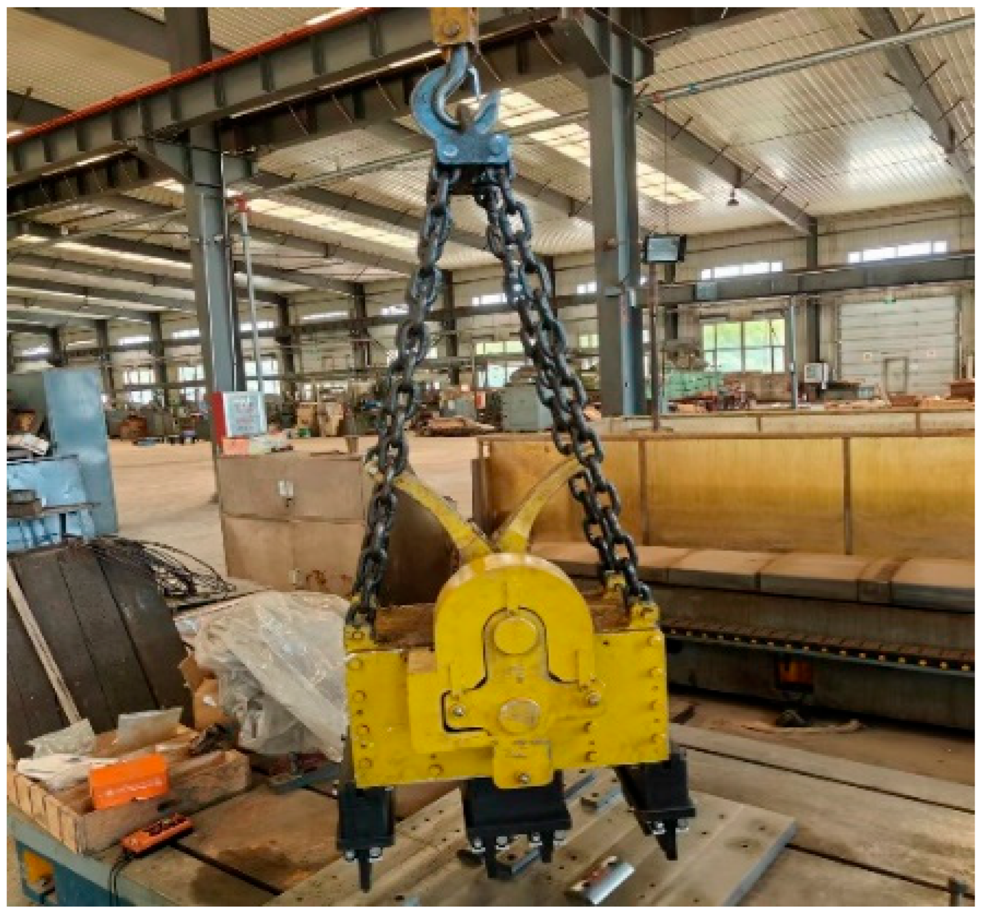
This type of permanent magnet, as shown in Figure 3, consists of a transmission mechanism, a magnetic system, and a movable pole face mechanism. The traditional transmission mechanism is composed of an internal gear mechanism (housed in a cover) and a chain hoist, which drives the rotation of composite permanent magnets in the magnetic system to achieve magnetic circuit switching. The magnetic system is made up of permanent magnets, conductors, and insulators, fulfilling the function of lifting heavy objects. The movable pole face mechanism comprises numerous movable magnetic poles, which can fit uneven surfaces to a greater extent and enhance the load-carrying capacity for workpieces with uneven surfaces. Based on its working principle, the FMEA is constructed, as shown in Table 1.
Three domain experts were invited to provide risk assessments in this case study. The selection criteria were rigorously defined to ensure the reliability and authority of the evaluations. All experts possess substantial professional experience (over 3 years) in relevant fields and are proficient in the FMEA methodology. Crucially, all experts were directly involved in the research and development of the specific multi-magnetic system lifting permanent magnets under investigation, guaranteeing that their assessments are grounded in profound system-specific knowledge. The detailed profiles of the experts are summarized in Table 2.
When conducting FBWM weight calculation, experts first provide the best and worst data, as shown in Table 3. Then, the data are processed using Formula (11) to obtain quantized results, which are presented in Table 4.
BWM weights are calculated based on the data provided in Table 4, yielding individual expert weights and comprehensive weights, as shown in Table 5. The weight of S is the highest, followed by O, and D is the lowest. The CR (Consistency Ratio) values of the three experts are 0.02666667, 0.00877578, and 0.01142857, respectively, which all less than 0.1, indicating that the consistency test is passed.
Three experts were invited to conduct a risk assessment on the multi-magnetic system lifting permanent magnets for uneven surfaces, and risk assessment values for each failure mode were obtained. The data are shown in Table 6.
Based on the RPN table provided by the experts, the O values provided in Table 6 are quantized using Formula (11). The geometric mean method is then adopted to aggregate the experts’ risk assessment data, resulting in the final O value of (27).
O s = { 5.116211 , 4.021056 , 4.156698 , 4.824871 , 4.389922 , 3.762889 , 3.774155 , 5.536702 , 5.511272 , 8.071689 , 7.2074 , 6.299471 }
In Section 3.1, the highest evaluation index defined by experts is nine. The O s is processed using Formula (17) to obtain the occurrence rate in probability form, denoted as O in Formula (28).
O = { 0.568468 , 0.446784 , 0.461855 , 0.536097 , 0.487769 , 0.418099 , 0.419351 , 0.615189 , 0.612364 , 0.896854 , 0.800822 , 0.699941 }
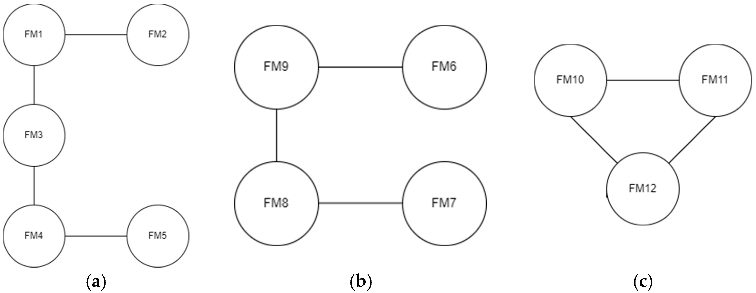
Three spatial structure distributions are listed for the transmission mechanism, magnetic system, and movable pole face mechanism, as shown in Figure 4.
Among all failure modes, the failed components around FM1, FM2, FM3, FM4, FM5, FM6, FM7, FM8, and FM9 are mutually independent, so the impact of the failure sequence of surrounding components on the results does not need to be considered. For FM10, FM11, and FM12, the failed components around them are interrelated, and the influence of the sequence must be taken into account. The final results obtained through calculation are shown in Formula (29).
O F = { 0.141741 , 0.28573 , 0.164211 , 0.145932 , 0.294178 , 0.288032 , 0.290227 , 0.190889 , 0.19032 , 0.65981 , 0.65981 , 0.65981 }
All RFs of the failure modes provided in Table 6 are quantized using Formula (11), and the geometric mean method is adopted to aggregate the risk assessment information from all experts, resulting in the values of S, O, and D. However, due to the different data scales between F and S, O, and D, the standardization process for S, O, D, and F is performed using Formula (21), and the final results are shown in Table 7.
Here, λ is introduced to integrate O * and O F * , with the specific formula shown in Formula (22). In this method, a compromise approach is adopted ( λ = 0.5 ) to synthesize O * and O F * , and the comprehensive weights of S, O, and D from Table 6 are integrated into the aforementioned result. The final outcomes are presented in the following table.
The data in Table 8 are processed using TOPSIS. First, Formula (25) is used to calculate the distance to the positive ideal solution D + and the distance to the negative ideal solution D for each scheme. Then, Formula (26) is applied to obtain the relative C i between each failure mode and the ideal solution. Finally, the risk ranking is determined based on the magnitude of Ci.
The final risk ranking, as presented in Table 9, provides a prioritized list for maintenance and design improvements. The high ranking of FM2 (Box Chain Fracture) and FM6 (Permanent Magnet Failure) as the top two critical failure modes is particularly noteworthy from an engineering perspective. FM2’s top position is attributed to its high S score, indicating that its failure would have a catastrophic impact on the system’s primary function of magnetic circuit switching. This aligns with engineering intuition, as a broken box chain would directly halt the lifting operation. Similarly, FM6 (Permanent Magnet Failure) ranks second due to its critical role in the magnetic system. A failure here would lead to a complete loss of lifting force, posing a severe safety hazard. The high ranking of these components underscores the need for robust design, high-quality materials, and preventative maintenance schedules specifically targeted at the chain assembly and permanent magnets to ensure operational safety and reliability.

4.2. Sensitivity Analysis

To evaluate the robustness of the proposed method and understand the impact of key parameters on the risk ranking results, a comprehensive sensitivity analysis was conducted. The focus was on the parameter r, which governs the weighting between the expert-evaluated O * and the load-sharing-derived O F * .
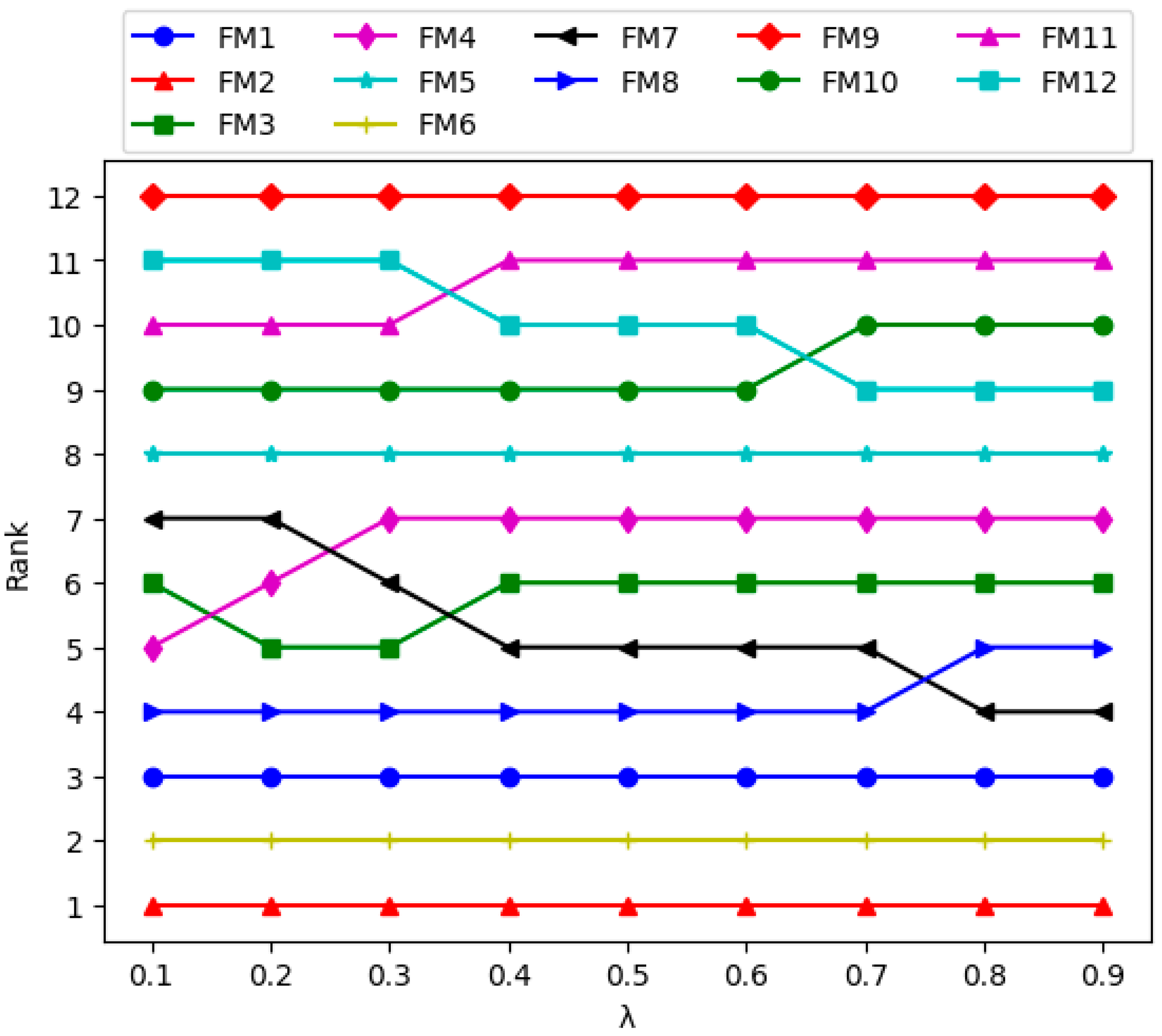
We adjust the value of λ and observe the changes in ranking under different proportions, with the results shown below (Figure 5).
As detailed in Table 10 and visualized in Figure 5, the failure mode rankings were calculated for a spectrum of λ values ranging from 0.1 to 0.9. The analysis reveals that the overall risk hierarchy is notably stable. Specifically, the top two failure modes (FM2 and FM6) and the bottom one (FM9) maintain their ranks across all scenarios. This stability in the extremities of the ranking list underscores the reliability of the proposed method in identifying the most critical and least critical failure modes, regardless of the chosen balance between subjective expert opinion and objective system structure data.
However, the analysis also provides valuable insights into how the system structure influences risk prioritization. The ranking of FM12 exhibits the most significant positive sensitivity to the parameter r. As r increases (giving more weight to the load sharing data O F * ), FM12’s rank consistently improves. This can be attributed to its two key characteristics: a high original expert-rated O value and few surrounding components in the spatial structure. In the load sharing model, a high O value combined with low redundancy (few components to share the load) results in a high O F * value, indicating a greater conditional probability of causing system failure. Consequently, as the influence of O F * grows, FM12 is correctly identified as a more significant risk.
Conversely, failure modes like FM4, FM8, and FM9 show a slight downward trend in their rankings as r increases. These components are typically surrounded by a larger number of adjacent components. This higher degree of redundancy within the system architecture means that their failure is less likely to lead to a system-wide collapse, as the load can be effectively redistributed. Therefore, their load-sharing-derived O F * is relatively lower, and when these objective data are given more weight, their perceived risk decreases appropriately.
The sensitivity of FM7 and FM10 further validates the model’s logical consistency. FM7, with fewer surrounding components, sees its rank increase with r, while FM10’s position remains relatively stable but high due to its critical structural role.
In conclusion, the sensitivity analysis demonstrates that the proposed model is not overly sensitive to the specific choice of the parameter r. The core ranking is robust, while the observed fluctuations for specific failure modes are not random noise but are logically explained by and provide valuable insight into the underlying system reliability physics. This enhances confidence in the method’s practical utility for engineers, as it consistently highlights critical failures while providing a nuanced understanding of how system design influences risk.

4.3. Comparative Experiment

To validate the effectiveness and superiority of the proposed load-sharing-based improved FMEA method, a comparative analysis was conducted against two classical approaches: the Traditional FMEA method, which ranks failure modes by directly multiplying the expert-rated S, O, and D values to obtain the RPN; and the PLTS-FBWM-TOPSIS method without load sharing, which employs the same PLTS for processing expert assessments, the FBWM for calculating weights, and TOPSIS for ranking, but does not incorporate any system data derived from load sharing. The comparative results are detailed in Table 11.
As can be seen from the above table, in the traditional FMEA method, FM8 ranks first and FM6 ranks second. Both FM6 and FM8 belong to the magnetic system. This ranking occurs because the traditional FMEA does not consider the weights of RFs. In the method without considering load sharing data, FM2 ranks first. Moreover, the rankings of FM4 and FM7 are quite different from those of the method proposed in this paper. This is because, when spatial factors are taken into account, FM4 is surrounded by more components, so its ranking rises, while FM7 has fewer surrounding components, leading to a decline in its ranking.
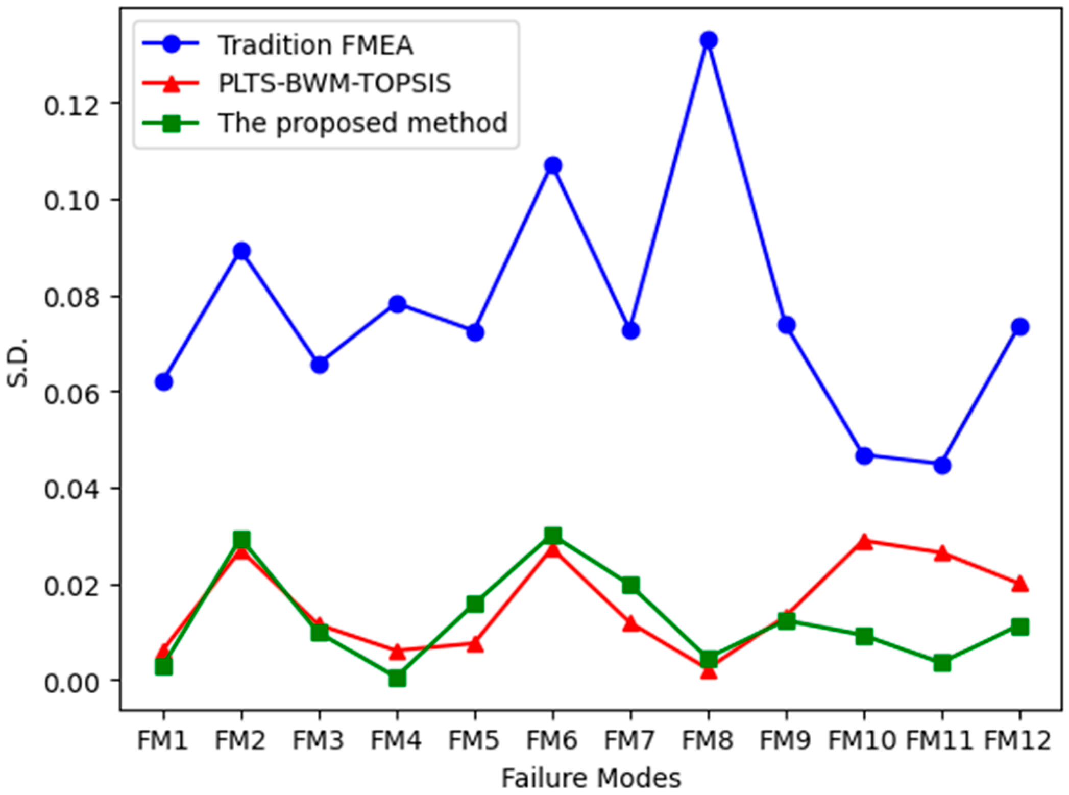
To verify the advantages of this method over other methods, we adjust the weights of S, O, and D: gradually reduce the weight of S by 0.01 and gradually increase the weight of O by 0.01, dividing into nine groups in total. We then calculate the standard deviation of C i for the nine groups. For the traditional FMEA method, we set the initial weights to be equal, and the specific details are shown in Table 12.
As shown in Figure 6, the analysis reveals that the standard deviations for all failure modes under the traditional FMEA method are substantially higher than those of the other two methods. This indicates that the traditional method is highly sensitive to the setting of risk factor weights; minor changes can lead to significant fluctuations in the ranking results, which is a major drawback in practical applications. In contrast, the PLTS-FBWM-TOPSIS method shows a marked reduction in standard deviation, demonstrating the enhanced stability offered by MCDM methods. Crucially, the proposed method achieves the smallest standard deviation for the majority of failure modes (e.g., FM1, FM4, FM8, FM10, FM11, and FM12). This provides strong evidence that the objective system structural information introduced by load sharing effectively counteracts the uncertainty inherent in subjective weight assignments, thereby endowing the overall risk assessment model with superior robustness.

5. Conclusions

This study addresses the limitations of traditional FMEA, such as neglecting inherent systemic structural information, equalizing RF weights, and a strong subjectivity in risk ranking, by proposing an improved FMEA method integrated with the load sharing principle. The method quantifies experts’ assessments using PLTS and aggregates multiple expert opinions via the geometric mean, determines the relative weights of S, O, and D with the FBWM, derives objective system failure probability data through load sharing modeling based on component spatial connections, and finally integrates subjective–objective data and weights into TOPSIS for comprehensive risk ranking. Validated on a multi-magnetic system magnetic crane, comparative experiments with traditional FMEA and PLTS-FBWM-TOPSIS confirm that the proposed method exhibits superior accuracy, stability, and objectivity in risk prioritization, providing reliable support for the risk assessment of complex multi-component systems.
In the future work, we want to integrate finite element analysis or multi-body dynamics simulation into expert evaluations to reduce the subjectivity in S, O, and D assessment, as well as expand the method’s application to load sharing systems like gearboxes and turbine rotors.

Author Contributions

B.S.: Writing—review and editing, Writing—original draft, Validation, Supervision, Resources, Project administration, Funding acquisition, Formal analysis, and Conceptualization. L.W.: Writing—original draft, Visualization, Validation, Software, Methodology, Investigation, Formal analysis, and Data curation. J.Z.: Supervision, Resources, Investigation, and Formal analysis. N.D.: Resources and Investigation. All authors have read and agreed to the published version of the manuscript.

Funding

This research was funded by the Jilin Provincial Science and Technology Development Plan, grant number YDZJ202401303ZYTS.

Data Availability Statement

Data will be made available on request.

Conflicts of Interest

The authors declare no conflicts of interest.

Appendix A

In Section 3.3, the expert-provided Occurrence (O) ratings are first quantified and aggregated. This aggregated value is then converted into its corresponding probabilistic form, denoted as E = { e 1 , e 2 , , e n } .

Appendix A.1. Derivation When Components Are Mutually Independent

Define the Failure Probability of the Next State:
The probability of transitioning from the initial state to the next failure mode is given by the set S. If no failure occurs, it is expressed as shown in Formula (A1).
e i = e j
Assume that when component j around component i fails, the load on component i will increase, and thus its probability of failure will rise, as expressed in Formula (A2).
e i ( j ) = ( 1 + z i ( j ) L ) e i
Assume that when component j fails, if the nearby components fail, the formula is as shown in Formula (A3).
e i ( j , k ) = ( 1 + z i ( j , k ) L ) e i
Under the condition of component independence, the final derived method is as follows:
F i ( j 1 , j 2 , j 3 , , j n ) = e j 1 × e j 2 ( j 1 ) × e j 3 ( j 1 , j 2 ) × × e j n ( j 1 , j 2 , , j n 1 ) × e i ( j 1 , j 2 , j n )

Appendix A.2. Derivation When Components Are Interrelated
In the single scenario described in Appendix A.1, the situation occurs only when the failed components j 1 , j 2 , j 3 , , j n are mutually independent. If there are m interrelated components among j 1 , j 2 , j 3 , , j n , different sequences of components may result in m! outcomes for F. In this section, we will address this issue by aggregating multiple outcomes into a single result.
Define the sequences of independent and interrelated components:
When there are n components around component i, there are n! possible sequences, as shown in Formula (A5). If these n components are mutually independent, changes in their sequence will have no impact, as shown in Formula (A6).
{ F i ( j 1 , j 2 , j 3 , , j n ) , F i ( j 2 , j 1 , j 3 , , j n ) , F i ( j 3 , j 2 , j 1 , , j n ) , , F i ( j n , j n 1 , j n 2 , , j 1 ) }
F i ( j 1 , j 2 , j 3 , , j n ) = F i ( j 2 , j 1 , j 3 , , j n ) = F i ( j 3 , j 2 , j 1 , , j n ) = = F i ( j n , j n 1 , j n 2 , , j 1 )
If, among these n components, m are interrelated with each other, there can be at most m! distinct outcomes for O. Since independent components have no impact on the result regardless of their positions, we divide O into two subsets: set A, consisting of interrelated components, and set B, consisting of mutually independent components, as shown in Formula (A7).
A = { a 1 , a 2 , , a m } B = { b 1 , b 2 , , b s } , m + s = n , F = { A , B }
Calculation of Independent Components:
Since the order of components in set B does not affect the result, we will only consider the order of components in set A as shown in Set (A8). Therefore, we derive the result for set B as shown in Formula (A9).
{ F i ( a 1 , a 2 , a 3 , , a m ) , F i ( a 2 , a 1 , a 3 , , a m ) , F i ( a 3 , a 2 , a 1 , , a m ) , , F i ( a m , a m 1 , a m 2 , , a 1 ) }
F B = e b 1 × e b 2 × × e b s
Calculation of All Sequential Values of F:
There are m! possible sequences for set A, as shown in Set (A10), and all corresponding results are presented in Formula (A11).
F s = { F i ( a 1 , a 2 , a 3 , , a m ) , F i ( a 2 , a 1 , a 3 , , a m ) , F i ( a 3 , a 2 , a 1 , , a m ) , , F i ( a m , a m 1 , a m 2 , , a 1 ) }
F i ( a 1 , a 2 , a 3 , , a m ) = e a 1 × e a 2 ( a 1 ) × × e a n ( a 1 , a 2 , , a m 1 ) × e i ( a 1 , a 2 , a m ) × F B F i ( a 2 , a 1 , a 3 , , a m ) = e a 2 × e a 1 ( a 2 ) × × e a n ( a 2 , a 1 , , a m 1 ) × e i ( a 2 , a 1 , a m ) × F B F i ( a 3 , a 2 , a 1 , , a m ) = e a 3 × e a 2 ( a 3 ) × × e a n ( a 3 , a 2 , , a m 1 ) × e i ( a 3 , a 2 , a m ) × F B F i ( a n , a n 1 , a n 2 , , a 1 ) = e a m × e a m 1 ( a m ) × × e a 1 ( a m , a m 1 , , a 2 ) × e i ( a m , a m 1 , a 1 ) × F B
Weight Calculation and Aggregation of All Different Sequences:
If there are m interrelated components among the n components, the results for all different sequences of the interrelated components are calculated using Formula (A4), as shown in Formula (A12). A larger value indicates a higher occurrence probability and thus a greater weight, with the weight calculation formula presented in Formula (A13).
D 1 = F ( a 1 , a 2 , a 3 , , a m ) = e a 1 × e a 2 ( a 1 ) × e a 3 ( a 1 , a 2 ) × × e a n ( a 1 , a 2 , , a m 1 ) D 2 = F ( a 2 , a 1 , a 3 , , a m ) = e a 2 × e a 1 ( a 2 ) × e a 3 ( a 2 , a 1 ) × × e a n ( a 2 , a 1 , , a m 1 ) D 3 = F ( a 3 , a 2 , a 1 , , a m ) = e a 3 × e a 2 ( a 3 ) × e a 1 ( a 3 , a 2 ) × × e a n ( a 3 , a 2 , , a m 1 ) D m ! = F ( a n , a n 1 , a n 2 , , a 1 ) = e a m × e a m 1 ( a m ) × e a m 2 ( a m , a m 1 ) × × e a 1 ( a m , a m 1 , , a 2 )
w i = D i i = 1 m ! D i
By weighted averaging w i into the set F s , the final aggregated result is obtained as shown in Formula (A14).
F i = w 1 × F i ( a 1 , a 2 , a 3 , , a m ) + w 2 × F i ( a 2 , a 1 , a 3 , , a m ) + , + w m ! × F i ( a m , a m 1 , a m 2 , , a 1 )
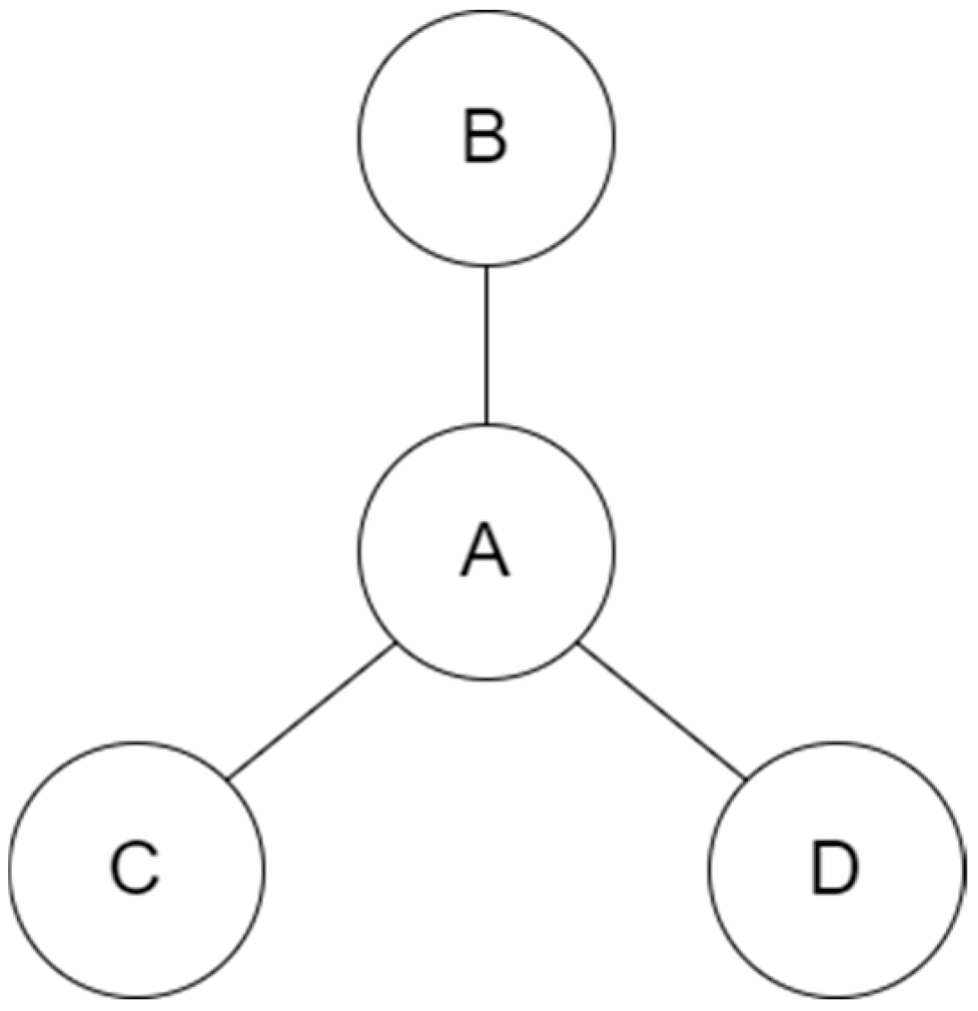
To illustrate how to calculate the occurrence probability of a failure mode, we use Figure A1 for description. Components B, C, and D are unconnected with no interrelationships, and they do not bear each other’s loads when failing. Only after B, C, and D fail simultaneously will the failure of Component A lead to system failure. B, C, and D are mutually independent, so their individual failures do not affect each other’s failure probabilities. After B, C, and D fail, Component A will bear the loads originally assigned to B, C, and D, resulting in increased load and a higher probability of failure. This is related to the proportion of loads that B, C, and D distribute to A. Calculating the data for A means determining the conditions under which A’s failure will cause system failure.
Figure A1. An unrelated Four-component system.
Machines 13 01113 g0a1
Calculate the occurrence probability F A = e B × e C × e D × e A ( B , C , D ) of Component A, where e B = e B * , e C = e C * , e D = e D * , e A ( B , C , D ) = ( 1 + z A ( B , C , D ) L ) e A .
The above calculation is based on the scenario where the surrounding components of the target component have no interrelationships and the failure sequence does not affect the final result. However, if the surrounding components are interrelated, different failure sequences will lead to different final results, as shown in Figure A2. When analyzing Component A, the failure sequence of Component B does not affect the final result, but the failures of Components C and D will affect their own loads, resulting in an increased probability of failure.
Figure A2. An unrelated Four-component system.
Machines 13 01113 g0a2
When Component C fails first and Component D subsequently fails, F A ( C , D ) = e B × e C × e D ( C ) × e A ( B , C , D ) . When Component D fails first and Component C subsequently fails, F A ( D , C ) = e B × e D × e C ( D ) × e A ( B , C , D ) .
To integrate these two scenarios, the one with a higher occurrence probability is assigned a greater weight. The weights of Components C and D are calculated as shown in Formula (A15).
w C = e C × e D ( C ) e C × e D ( C ) + e D × e C ( D ) w D = e D × e C ( D ) e C × e D ( C ) + e D × e C ( D )
The final simplified result is F A = w C F A ( C , D ) + w D F A ( D , C ) .

References

  1. Wang, L.; Li, B.; Hu, B.; Shen, G.; Zheng, Y.; Zheng, Y. Failure mode effect and criticality analysis of ultrasound device by classification tracking. BMC Health Serv. Res. 2022, 22, 429. [Google Scholar] [CrossRef]
  2. Wu, Z.; Liu, W.; Nie, W. Literature review and prospect of the development and application of FMEA in manufacturing industry. Int. J. Adv. Manuf. Technol. 2021, 112, 1409–1436. [Google Scholar] [CrossRef]
  3. Naranjo, J.E.; Alban, J.S.; Balseca, M.S.; Bustamante Villagómez, D.F.; Mancheno Falconi, M.G.; Garcia, M.V.J.S. Enhancing Institutional Sustainability Through Process Optimization: A Hybrid Approach Using FMEA and Machine Learning. Int. J. Adv. Manuf. Technol. 2025, 17, 1357. [Google Scholar] [CrossRef]
  4. Shi, H.; Wang, L.; Li, X.-Y.; Liu, H.-C. A novel method for failure mode and effects analysis using fuzzy evidential reasoning and fuzzy Petri nets. J. Ambient Intell. Humaniz. Comput. 2020, 11, 2381–2395. [Google Scholar] [CrossRef]
  5. Tian, Y.; Song, S.; Zhou, D.; Pang, S.; Wei, C. Canonical triangular interval type-2 fuzzy set linguistic distribution assessment TODIM approach: A case study of FMEA for electric vehicles DC charging piles. Expert Syst. Appl. 2023, 223, 119826. [Google Scholar] [CrossRef]
  6. Li, A. Risk assessment of crane operation hazards using modified FMEA approach with Z-Number and set pair analysis. Heliyon 2024, 10, e28603. [Google Scholar] [CrossRef]
  7. Pang, Q.; Wang, H.; Xu, Z. Probabilistic linguistic term sets in multi-attribute group decision making. Inf. Sci. 2016, 369, 128–143. [Google Scholar] [CrossRef]
  8. Farhadinia, B.; Liao, H. Group decision making based on the relationships between the information measures for additive and multiplicative linguistic term sets. Soft Comput. 2019, 23, 7901–7911. [Google Scholar] [CrossRef]
  9. Ma, X.; Han, X.; Xu, Z.; Rodriguez, R.M.; Zhan, J. Fusion of probabilistic linguistic term sets for enhanced group decision-making: Foundations, survey and challenges. Inf. Fusion 2025, 116, 102802. [Google Scholar] [CrossRef]
  10. Gou, X.; Xu, Z.; Liao, H.; Herrera, F. Probabilistic double hierarchy linguistic term set and its use in designing an improved VIKOR method: The application in smart healthcare. J. Oper. Res. Soc. 2021, 72, 2611–2630. [Google Scholar] [CrossRef]
  11. Wang, Z.-C.; Ran, Y.; Chen, Y.; Yang, X.; Zhang, G. Group risk assessment in failure mode and effects analysis using a hybrid probabilistic hesitant fuzzy linguistic MCDM method. Expert Syst. Appl. 2022, 188, 116013. [Google Scholar] [CrossRef]
  12. Lo, H.-W.; Shiue, W.; Liou, J.J.; Tzeng, G.-H. A hybrid MCDM-based FMEA model for identification of critical failure modes in manufacturing. Soft Comput. 2020, 24, 15733–15745. [Google Scholar] [CrossRef]
  13. Kumari, S.; Ahmad, K.; Khan, Z.A.; Ahmad, S. Analysing the failure modes of water treatment plant using FMEA based on fuzzy AHP and fuzzy VIKOR methods. Arab. J. Sci. Eng. 2025, 50, 16821–16836. [Google Scholar] [CrossRef]
  14. Li, H.; Díaz, H.; Soares, C. A failure analysis of floating offshore wind turbines using AHP-FMEA methodology. Ocean Eng. 2021, 234, 109261. [Google Scholar] [CrossRef]
  15. Rezaei, J. Best-worst multi-criteria decision-making method. Omega 2015, 53, 49–57. [Google Scholar] [CrossRef]
  16. Pamučar, D.; Ecer, F.; Cirovic, G.; Arlasheedi, M. Application of improved best worst method (BWM) in real-world problems. Mathematics 2020, 8, 1342. [Google Scholar] [CrossRef]
  17. Liou, J.J.; Guo, B.H.; Huang, S.-W.; Yang, Y.-T. Failure mode and effect analysis using interval type-2 fuzzy and multiple-criteria decision-making methods. Mathematics 2024, 12, 3931. [Google Scholar] [CrossRef]
  18. Xue, Y.; Zhang, J.; Zhang, Y.; Yu, X. Barrier assessment of EV business model innovation in China: An MCDM-based FMEA. Transp. Environ. 2024, 136, 104404. [Google Scholar] [CrossRef]
  19. Kuchekar, P.; Bhongade, A.S.; Rehman, A.U.; Mian, S.H. Assessing the Critical Factors Leading to the Failure of the Industrial Pressure Relief Valve Through a Hybrid MCDM-FMEA Approach. Machines 2024, 12, 820. [Google Scholar] [CrossRef]
  20. Shafizadeh, E.; Hossein Mousavizadegan, S. A comprehensive risk assessment framework for composite Lenj Hulls: Integrating FMEA with CRITIC-CODAS. Civ. Eng. Environ. Syst. 2025, 1–21. [Google Scholar] [CrossRef]
  21. Wang, J.; Zhang, J.; Wu, J.; Zhang, Q.; Fang, Y.; Huang, X. Optimal inspection-based maintenance strategy for k-out-of-n: G load-sharing systems consisting of three-state components. Comput. Ind. Eng. 2025, 209, 111446. [Google Scholar] [CrossRef]
  22. Singh, B.; Gupta, P.K. Load-sharing system model and its application to the real data set. Math. Comput. Simul. 2012, 82, 1615–1629. [Google Scholar] [CrossRef]
  23. Seikh, M.R.; Chatterjee, P. Sustainable strategies for electric vehicle adoption: A confidence level-based interval-valued spherical fuzzy MEREC-VIKOR approach. Inf. Sci. 2025, 699, 121814. [Google Scholar] [CrossRef]
  24. Al-Abadi, A.M.; Handhal, A.M.; Abdulhasan, M.A.; Ali, W.L.; Hassan, J.; Al Aboodi, A.H. Optimal siting of large photovoltaic solar farms at Basrah governorate, Southern Iraq using hybrid GIS-based Entropy-TOPSIS and AHP-TOPSIS models. Renew. Energy 2025, 241, 122308. [Google Scholar] [CrossRef]
  25. Behzadian, M.; Otaghsara, S.K.; Yazdani, M.; Ignatius, J. A state-of the-art survey of TOPSIS applications. Expert Syst. Appl. 2012, 39, 13051–13069. [Google Scholar] [CrossRef]
  26. Zhao, S.; Wei, Y.; Li, Y.; Cheng, Y. A multi-agent reinforcement learning (MARL) framework for designing an optimal state-specific hybrid maintenance policy for a series k-out-of-n load-sharing system. Reliab. Eng. Syst. Saf. 2025, 265, 111587. [Google Scholar] [CrossRef]
  27. Krejčí, J.; Stoklasa, J. Aggregation in the analytic hierarchy process: Why weighted geometric mean should be used instead of weighted arithmetic mean. Expert Syst. Appl. 2018, 114, 97–106. [Google Scholar] [CrossRef]
  28. Bahrami, S.; Rastegar, M.; Dehghanian, P. An fbwm-topsis approach to identify critical feeders for reliability centered maintenance in power distribution systems. Manuf. Rev. 2020, 15, 3893–3901. [Google Scholar] [CrossRef]
  29. Xiao, Z.; Shi, Z.; Bai, J. FMEA Risk Assessment Method for Aircraft Power Supply System Based on Probabilistic Language-TOPSIS. Aerospace 2025, 12, 548. [Google Scholar] [CrossRef]
  30. Trung, D.D. Development of data normalization methods for multi-criteria decision making: Applying for MARCOS method. Manuf. Rev. 2022, 9, 22. [Google Scholar] [CrossRef]
  31. Zhou, X.; Tang, Y. Modeling and fusing the uncertainty of FMEA experts using an entropy-like measure with an application in fault evaluation of aircraft turbine rotor blades. Entropy 2018, 20, 864. [Google Scholar] [CrossRef] [PubMed]
  32. Zhuo, Y.; Ma, L.; Li, C.; Chen, X. Risk analysis and mitigation of pressurization test for civil aircraft airtight cabin doors based on FMEA. J. Phys. Conf. Ser. 2025, 3080, 012142. [Google Scholar] [CrossRef]
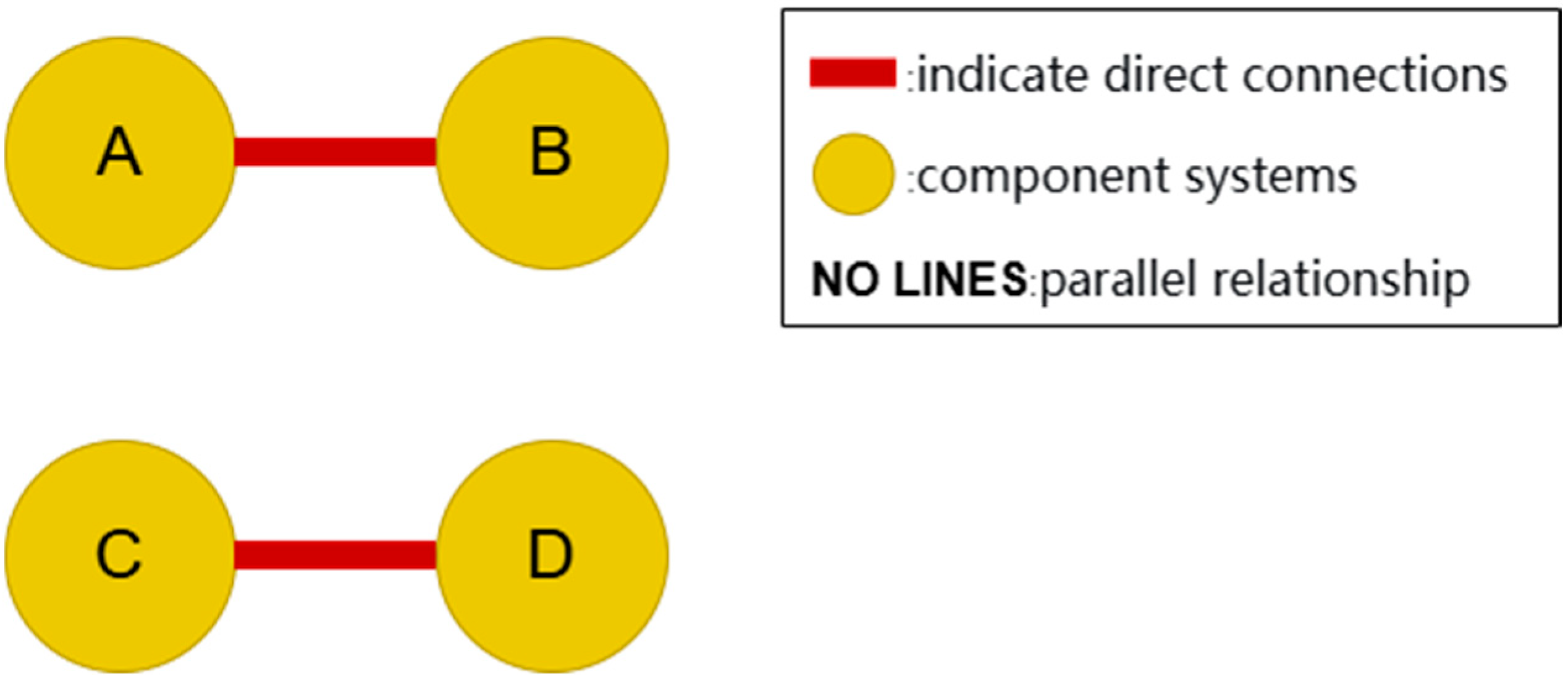
Figure 1. Four-component system.
Machines 13 01113 g001
Figure 2. Methodology flow chart.
Machines 13 01113 g002
Figure 3. Actual scene diagram of the multi-magnetic system lifting permanent magnets for uneven surfaces.
Machines 13 01113 g003
Figure 4. Spatial relationship of failure modes. (a) Transmission mechanism; (b) Magnetic system; (c) Movable pole face mechanism.
Machines 13 01113 g004
Figure 5. Visualization results of rankings under different λ values.
Machines 13 01113 g005
Figure 6. Standard deviation of failure modes under different methods.
Machines 13 01113 g006
Table 1. FMEA failure modes of the multi-magnetic system lifting permanent magnets for uneven surfaces.
Structure GroupFunctionItemFailed Component
Transmission
Mechanism
Magnetic Circuit SwitchingFM1Ratcheting Chain Fracture
FM2Box Chain Fracture
FM3Ratchet Wear
FM4Gear Wear
FM5Rotating Shaft Wear
Magnetic
System
Lifting Heavy ObjectsFM6Permanent Magnet Failure
FM7Outer Yoke Failure
FM8Inner Yoke Failure
FM9Pole Shoe Failure
Movable Pole
Face Mechanism
Achieve a higher degree of fit with the workpiece surfaceFM10T-Type Movable Pole Jamming
FM11Stopper Movable Pole Jamming
FM12Cam Jamming
Table 2. Expert’s information.
ExpertExperienceYears of Study
EX1Responsible for the full-cycle development of the multi-magnetic system lifting permanent magnets, from design to manufacturing10
EX2The critical optimization of the movable pole face mechanism3
EX3Design phase of the movable pole face mechanism3
Table 3. Experts’ RFs risk assessment information.
BestSODSODWorst
EX1S { ( m 1 , p 1 ) } { ( m 2 , 1 p 2 ) , ( m 3 , p 2 ) } { ( m 6 , p 4 ) , ( m 5 , 1 p 4 ) } { ( m 6 , p 4 ) , ( m 5 , 1 p 4 ) } { ( m 2 , p 2 ) , ( m 3 , 1 p 2 ) } { ( m 1 , p 1 ) } D
EX2S { ( m 1 , p 1 ) } { ( m 2 , p 4 ) , ( m 3 , 1 p 4 ) } { ( m 5 , p 3 ) , ( m 6 , 1 p 3 ) } { ( m 5 , p 3 ) , ( m 6 , 1 p 3 ) } { ( m 2 , p 2 ) , ( m 3 , 1 p 2 ) } { ( m 1 , p 1 ) } D
EX3S { ( m 1 , p 1 ) } { ( m 1 , 1 p 2 ) , ( m 2 , p 2 ) } { ( m 3 , p 4 ) , ( m 4 , 1 p 4 ) } { ( m 3 , p 4 ) , ( m 4 , 1 p 4 ) } { ( m 1 , p 4 ) , ( m 3 , 1 p 4 ) } { ( m 1 , p 1 ) } D
Table 4. Quantized RF comparison data.
BestSODSODWorst
EX1S12.85.55.52.21D
EX2S12.55.35.32.21D
EX3S11.83.53.521D
Table 5. Weights of RFs.
w S w O w D CR
EX10.647988510.237068970.114942530.02666667
EX20.628758170.253594770.117647060.00877578
EX30.542510120.303643720.153846150.01142857
0.6073040110.2644719730.128224016
Table 6. RPN table of the multi-magnetic system lifting permanent magnets for uneven surfaces.
SOD
FM1EX1 { ( s 4 , p 2 ) , ( s 5 , 1 p 2 ) } { ( s 6 , p 2 ) , ( s 7 , 1 p 2 ) } { ( s 2 , p 2 ) , ( s 3 , 1 p 2 ) }
EX2 { ( s 5 , p 1 ) } { ( s 5 , p 2 ) , ( s 4 , 1 p 2 ) } { ( s 3 , p 2 ) }
EX3 { ( s 5 , p 3 ) , ( s 6 , 1 p 3 ) } { ( s 5 , p 1 ) } { ( s 2 , p 4 ) , ( s 3 , 1 p 4 ) }
FM2EX1 { ( s 9 , p 3 ) , ( s 8 , 1 p 3 ) } { ( s 4 , p 3 ) , ( s 5 , 1 p 3 ) } { ( s 2 , p 4 ) , ( s 3 , 1 p 4 ) }
EX2 { ( s 8 , p 1 ) } { ( s 4 , p 2 ) , ( s 5 , 1 p 2 ) } { ( s 2 , p 2 ) , ( s 3 , 1 p 2 ) }
EX3 { ( s 9 , p 2 ) } { ( s 4 , p 1 ) } { ( s 3 , p 3 ) , ( s 4 , 1 p 3 ) }
FM3EX1 { ( s 4 , p 2 ) , ( s 5 , 1 p 2 ) } { ( s 4 , p 4 ) , ( s 5 , 1 p 4 ) } { ( s 3 , p 4 ) , ( s 4 , 1 p 4 ) }
EX2 { ( s 5 , p 2 ) , ( s 6 , 1 p 2 ) } { ( s 4 , p 2 ) , ( s 5 , 1 p 2 ) } { ( s 3 , p 2 ) }
EX3 { ( s 5 , p 2 ) } { ( s 4 , p 2 ) , ( s 3 , 1 p 2 ) } { ( s 5 , p 2 ) }
FM4EX1 { ( s 4 , p 2 ) , ( s 5 , 1 p 2 ) } { ( s 5 , p 2 ) , ( s 6 , 1 p 2 ) } { ( s 3 , p 4 ) , ( s 4 , 1 p 4 ) }
EX2 { ( s 5 , p 1 ) } { ( s 5 , p 1 ) } { ( s 4 , p 2 ) }
EX3 { ( s 4 , p 3 ) , ( s 5 , 1 p 3 ) } { ( s 6 , p 2 ) } { ( s 3 , p 4 ) , ( s 4 , 1 p 4 ) }
FM5EX1 { ( s 5 , p 2 ) , ( s 4 , 1 p 2 ) } { ( s 5 , p 3 ) , ( s 4 , 1 p 3 ) } { ( s 3 , p 4 ) , ( s 5 , 1 p 4 ) }
EX2 { ( s 5 , p 1 ) } { ( s 5 , p 2 ) } { ( s 4 , p 2 ) , ( s 3 , 1 p 2 ) }
EX3 { ( s 3 , p 2 ) , ( s 4 , 1 p 2 ) } { ( s 5 , p 1 ) } { ( s 4 , p 2 ) }
FM6EX1 { ( s 7 , p 2 ) , ( s 8 , 1 p 2 ) } { ( s 4 , p 3 ) , ( s 3 , 1 p 3 ) } { ( s 3 , p 2 ) , ( s 4 , 1 p 2 ) }
EX2 { ( s 7 , p 1 ) } { ( s 3 , p 2 ) , ( s 4 , 1 p 2 ) } { ( s 6 , p 2 ) , ( s 5 , 1 p 2 ) }
EX3 { ( s 8 , p 2 ) } { ( s 5 , p 1 ) } { ( s 4 , p 2 ) }
FM7EX1 { ( s 3 , p 4 ) , ( s 4 , 1 p 4 ) } { ( s 4 , p 2 ) , ( s 5 , 1 p 2 ) } { ( s 4 , p 2 ) , ( s 5 , 1 p 2 ) }
EX2 { ( s 4 , p 2 ) , ( s 3 , 1 p 2 ) } { ( s 3 , p 2 ) , ( s 4 , 1 p 2 ) } { ( s 5 , p 4 ) , ( s 6 , 1 p 4 ) }
EX3 { ( s 6 , p 2 ) , ( s 7 , 1 p 2 ) } { ( s 5 , p 2 ) } { ( s 3 , p 2 ) , ( s 2 , 1 p 2 ) }
FM8EX1 { ( s 3 , p 4 ) , ( s 5 , 1 p 4 ) } { ( s 5 , p 2 ) , ( s 6 , 1 p 2 ) } { ( s 5 , p 2 ) , ( s 6 , 1 p 2 ) }
EX2 { ( s 4 , p 4 ) , ( s 5 , 1 p 4 ) } { ( s 6 , p 2 ) } { ( s 6 , p 4 ) , ( s 5 , 1 p 4 ) }
EX3 { ( s 4 , p 2 ) , ( s 5 , 1 p 2 ) } { ( s 7 , p 2 ) , ( s 6 , 1 p 2 ) } { ( s 6 , p 2 ) }
FM9EX1 { ( s 3 , p 2 ) , ( s 4 , 1 p 2 ) } { ( s 5 , p 4 ) , ( s 7 , 1 p 4 ) } { ( s 6 , p 2 ) , ( s 5 , 1 p 2 ) }
EX2 { ( s 2 , p 2 ) , ( s 1 , 1 p 2 ) } { ( s 6 , p 2 ) , ( s 7 , 1 p 2 ) } { ( s 5 , p 2 ) }
EX3 { ( s 3 , p 2 ) } { ( s 5 , p 1 ) } { ( s 7 , p 2 ) }
FM10EX1 { ( s 2 , p 4 ) , ( s 3 , 1 p 4 ) } { ( s 8 , p 3 ) , ( s 9 , 1 p 3 ) } { ( s 2 , p 2 ) , ( s 3 , 1 p 2 ) }
EX2 { ( s 2 , p 2 ) , ( s 3 , 1 p 2 ) } { ( s 9 , p 2 ) } { ( s 2 , p 2 ) , ( s 1 , 1 p 2 ) }
EX3 { ( s 2 , p 1 ) } { ( s 9 , p 2 ) , ( s 8 , 1 p 2 ) } { ( s 4 , p 3 ) , ( s 3 , 1 p 3 ) }
FM11EX1 { ( s 2 , p 2 ) , ( s 3 , 1 p 2 ) } { ( s 7 , p 4 ) , ( s 8 , 1 p 4 ) } { ( s 2 , p 4 ) , ( s 3 , 1 p 4 ) }
EX2 { ( s 3 , p 1 ) } { ( s 8 , p 2 ) , ( s 7 , 1 p 2 ) } { ( s 3 , p 2 ) }
EX3 { ( s 2 , p 1 ) } { ( s 8 , p 2 ) } { ( s 3 , p 2 ) , ( s 2 , 1 p 2 ) }
FM12EX1 { ( s 2 , p 2 ) , ( s 3 , 1 p 2 ) } { ( s 6 , p 2 ) , ( s 7 , 1 p 2 ) } { ( s 4 , p 2 ) , ( s 5 , 1 p 2 ) }
EX2 { ( s 2 , p 4 ) , ( s 3 , 1 p 4 ) } { ( s 7 , p 2 ) , ( s 8 , 1 p 2 ) } { ( s 6 , p 2 ) , ( s 5 , 1 p 2 ) }
EX3 { ( s 2 , p 2 ) , ( s 3 , 1 p 2 ) } { ( s 7 , p 2 ) } { ( s 5 , p 2 ) }
Table 7. Standardized RPN table.
S * O F * O * D *
FM10.4532230.0010.3150830.001
FM21.0010.2789340.0609160.095683
FM30.4157220.0443720.0923960.309919
FM40.3965970.0090890.2474680.370786
FM50.3553750.295240.1465240.46141
FM60.8113090.2833770.0010.551302
FM70.4004070.2876150.0036150.591554
FM80.3779120.0958680.4126721.001
FM90.0467790.0947680.406770.967412
FM100.0011.0011.0010.030928
FM110.0111051.0010.8004130.071771
FM120.0279021.0010.5896980.801735
Table 8. RPN table after FBWM processing.
SOD
FM10.2752440.0417980.000128
FM20.6079110.044940.012269
FM30.252470.0180860.039739
FM40.2408550.0339260.047544
FM50.2158210.0584170.059164
FM60.4927110.0376050.07069
FM70.2431690.0385110.075851
FM80.2295070.0672470.128352
FM90.0284090.0663210.124045
FM100.0006070.2647360.003966
FM110.0067440.2382120.009203
FM120.0169450.2103480.102802
Table 9. Risk ranking of all failure modes.
D + D C i RANK
FM10.4204880.2756590.3959783
FM20.2485670.6080190.7098161
FM30.4416190.2549580.3660156
FM40.441060.2453940.357487
FM50.448430.2267790.3358658
FM60.2611220.497520.6558032
FM70.4324020.2549260.3708955
FM80.4268390.2669340.3847574
FM90.6125440.135850.18152212
FM100.6199110.2466810.2846569
FM110.6134350.2203980.2643211
FM120.5940140.2185710.26898310
Table 10. Rankings under different λ values.
λ FM1FM2FM3FM4FM5FM6FM7FM8FM9FM10FM11FM12
10.1316582741291011
20.2315682741291011
30.3315782641291011
40.4316782541291110
50.5316782541291110
60.6316782541291110
70.7316782541210119
80.8316782451210119
90.9316782451210119
Table 11. Ranking results under different methods.
FMEAPLTS-FBWM-TOPSISThis Method
ScoreRANK C i RANK C i RANK
FM156.15464100.41768130.3959783
FM281.0389330.68890810.7098161
FM359.5158290.36891360.3660156
FM470.9944640.37330750.357487
FM565.7641580.33094980.3358658
FM697.2109220.62824120.6558032
FM765.941370.3592770.3708955
FM8120.770510.40977840.3847574
FM966.9918150.216856120.18152212
FM1042.41067110.29906990.2846569
FM1140.6663120.256036100.2643211
FM1266.5495260.237386110.26898310
Table 12. Comparison of different methods.
FMEAPLTS-FBWM-TOPSISThis Method
S.D.S.D.S.D.
FM10.0619560.0060720.002804
FM20.0894110.026950.029429
FM30.0656640.0114180.009803
FM40.0783290.006050.0005
FM50.0725580.007550.015694
FM60.1072530.027270.030127
FM70.0727530.0118930.019782
FM80.1332470.0022380.004481
FM90.0739120.0131170.012297
FM100.0467920.0289290.009267
FM110.0448670.0264420.003473
FM120.0734240.0200270.011247
Disclaimer/Publisher’s Note: The statements, opinions and data contained in all publications are solely those of the individual author(s) and contributor(s) and not of MDPI and/or the editor(s). MDPI and/or the editor(s) disclaim responsibility for any injury to people or property resulting from any ideas, methods, instructions or products referred to in the content.