Speed Independent Health Indicator for Outer Raceway Bearing Fault Using MCSA ^†

Abstract

Bearing health monitoring is essential for ensuring the reliability and operational safety of induction machines, as bearing faults remain among the most frequent failure modes in rotating electrical equipment. This work contributes to condition monitoring by enhancing the robustness of health indicators and developing a supply-frequency-independent health indicator (HI) for bearing fault diagnosis using Motor Current Signature Analysis (MCSA). The objective is to design an HI capable of reliably representing the bearing degradation state under varying operating conditions, particularly when the supply frequency changes. To achieve this, the study briefly examines the key physical mechanisms governing the detectability of bearing-related spectral signatures—including rotational frequency, unbalanced magnetic pull, eddy currents, skin effect, and hydrodynamic forces. The theoretical analysis establishes the overall trend expected under varying supply frequencies and clarifies how these phenomena collectively influence the spectral characteristics of the fault components and the frequency-dependent evolution of their amplitudes. These insights are experimentally validated using induction machines fitted with bearings of two fault severities. Leveraging this physical understanding, a modified regression-based compensation model is introduced to reduce the frequency-dependent variation in the HI. The resulting compensating factor effectively stabilizes the frequency response, producing a more consistent and monotonic degradation trend across the tested conditions. The proposed method is computationally lightweight, does not require run-to-failure data or detailed physical modeling, and is suitable for real-time implementation. By integrating physical insight with data-driven modeling, this work presents a practical and frequency-independent HI framework that can be readily deployed within digital-twin-based condition monitoring architectures for induction machines.

1. Introduction

Induction machines (IMs) are widely used in industrial and domestic systems because of their high efficiency, power density, and durability, making condition monitoring essential to avoid unexpected failures and the associated costs. Early detection is particularly important, as undiagnosed faults can propagate and cause secondary damage.

IMs can experience various faults—stator winding defects, broken rotor bars, shaft misalignment, and housing cracks—with bearing faults being the most common, representing nearly 40% of total failures, as reported by Alsaedi [1]. These faults belong to the class of eccentricity-related issues, where localized defects introduce periodic air-gap variations that distort magnetic flux and manifest in measurable quantities such as stator current, torque, and flux. Analyzing these signals can give an estimate for fault severity assessment and remaining useful life (RUL) estimation. Other eccentricity-related faults include shaft misalignment and rotor imbalance.

Conventional bearing diagnostics rely primarily on vibration captured by accelerometers, as considered by Spirto et al. [2], Marticorena and Peyrano [3], and Wen et al. [4], and, in some cases, torque sensors, microphones or external flux probes; however, these methods require additional hardware and frequently encounter installation constraints and signal attenuation issues, as reviewed by Nandi and Toliyat [5]. In contrast, Guo et al. [6] showed that Motor Current Signature Analysis (MCSA) provides a cost-effective alternative in which the machine effectively serves as its own sensor, allowing fault-induced disturbances to appear directly in the current spectrum. As it only requires a high-resolution DAQ system, MCSA eliminates the limitations of external sensors and offers an efficient, scalable diagnostic approach.

Efficient diagnostics further depend on computationally lightweight algorithms capable of processing large datasets rapidly, which is critical for online monitoring and digital-twin applications. Higher computational demand increases hardware cost and latency, as discussed by Amitabh et al. [7]. Thus, method selection must balance accuracy with practical feasibility.

Barbieri et al. [8] noted that prognostics of rotating machinery typically encompasses three major tasks: fault detection, fault severity assessment, and remaining useful life (RUL) estimation. A substantial body of literature, including the review by Nandi and Toliyat [5], demonstrates that bearing defects generate characteristic signatures in the stator current. These signatures commonly manifest at ball-pass-related frequencies and can be readily identified using frequency-domain approaches such as the Fast Fourier Transform (FFT). To improve feature extraction beyond classical spectral analysis, numerous advanced signal-processing techniques have been developed. Methods based on the Hilbert–Huang Transform and Park Vector Transform have been investigated by Bórnea et al. [9], while Song et al. [10] employed EEMD and CEEMDAN. Statistical learning-based approaches were explored by Yuvaraj et al. [11], and wavelet and time–frequency representations were used by Blodt et al. [12]. Furthermore, Li et al. [13] proposed dimensionality reduction techniques such as Principal Component Analysis (PCA) to enhance the isolation of fault-related components.

With recent advancements in computational power, data-driven approaches have gained substantial momentum in bearing fault diagnostics. A wide range of neural network architectures, support vector machines (SVM), and regression-based models have been investigated in the literature by various authors, including Filippetti et al. [14], Hu et al. [15], Ran et al. [16], Chen et al. [17], ElSayed [18], and Xie et al. [19]. These techniques extract patterns directly from measurement data and assess deviations from healthy operating conditions to identify emerging faults. Data-driven methods currently constitute the state of the art, particularly in vibration-based condition monitoring. However, despite their strong performance, these approaches do not inherently capture the physical causality of the system. As a result, their reliability can degrade when faced with operating conditions or measurement scenarios that fall outside the distribution of the training data. This raises the risk that a purely data-driven model may fail to generalize to previously unseen conditions.

Complementing these data-driven developments, detailed model-based studies incorporate explicit representations of bearing defects into machine electromechanical models to improve physical understanding and provide validation frameworks for diagnostic algorithms. Examples include the work of Amitabh et al. [20], Blodt et al. [21], Kripakaran and Reddy [22], Koti et al. [23], Ojaghi and Sabouri [24], and Kaikaa and Kecita [25].

However, most existing studies (mentioned above) do not adequately address the impact of varying operating conditions. While many works are limited to merely identifying the presence of bearing fault frequencies in the current spectrum, others estimate the machine’s health only at a fixed operating speed. In real-world applications, however, machines rarely operate under constant speed or load conditions. Consequently, health indicators derived under fixed conditions may become ineffective, as operating variations can introduce coupling effects that obscure the true relationship between the health indicator and bearing degradation. Ideally, a robust health indicator should vary solely with the degradation state of the bearing and remain insensitive to changes in operating parameters. In practice, however, completely isolating this effect is challenging, since tracing the entire signal propagation path through multiple machine components is inherently complex. Therefore, such influences can only be minimized rather than being eliminated.

To overcome this problem, several studies in the past have attempted to construct health indicators (HIs) that remain robust under variable operating conditions. Zimroz et al. [26] proposed a linear model between the feature value (RMS) of vibration and the turbine’s power output to mitigate variations in the HI for bearing fault diagnosis, assuming that such variations follow a linear trend. Li et al. [27] employed a two-factor state-space model to predict the remaining useful life (RUL) of bearings, using vibration data collected from accelerated degradation tests conducted at two discrete speeds. The study by Luo et al. [28] introduced an improved phase-space warping (IPSW) method and applied it to three bearings with seeded faults, where different rotational speeds were imposed to simulate stepwise degradation. Kim et al. [29] constructed a robust HI using Spearman correlation and Mahalanobis distance for run-to-failure vibration data obtained under two operating conditions with varying speeds. Singh et al. [30] decomposed vibration signals using Ensemble Empirical Mode Decomposition (EEMD) to suppress the influence of variable conditions on the HI. Meanwhile, studies by Koutroulis et al. [31], Li et al. [32], and He et al. [33] adopted predominantly data-driven approaches to assess health degradation and fault severity under time-varying operating conditions.

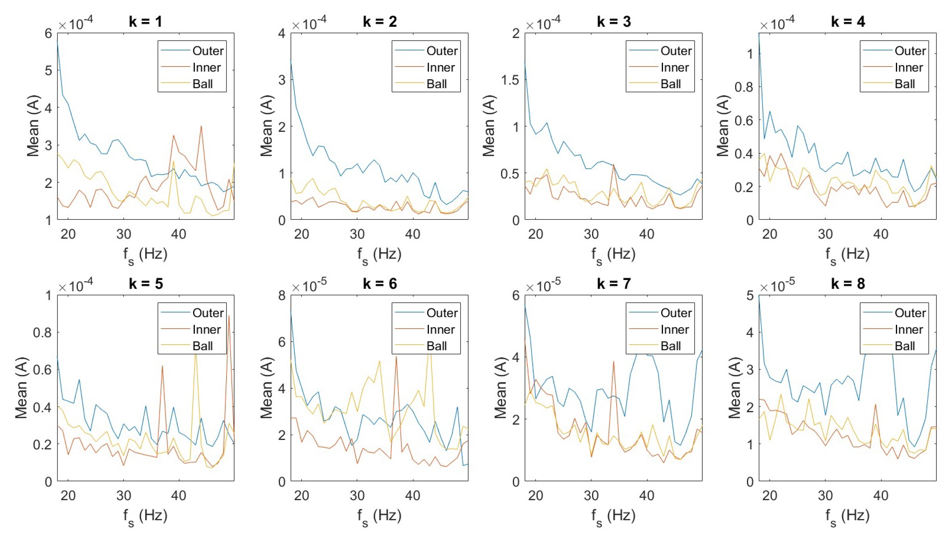
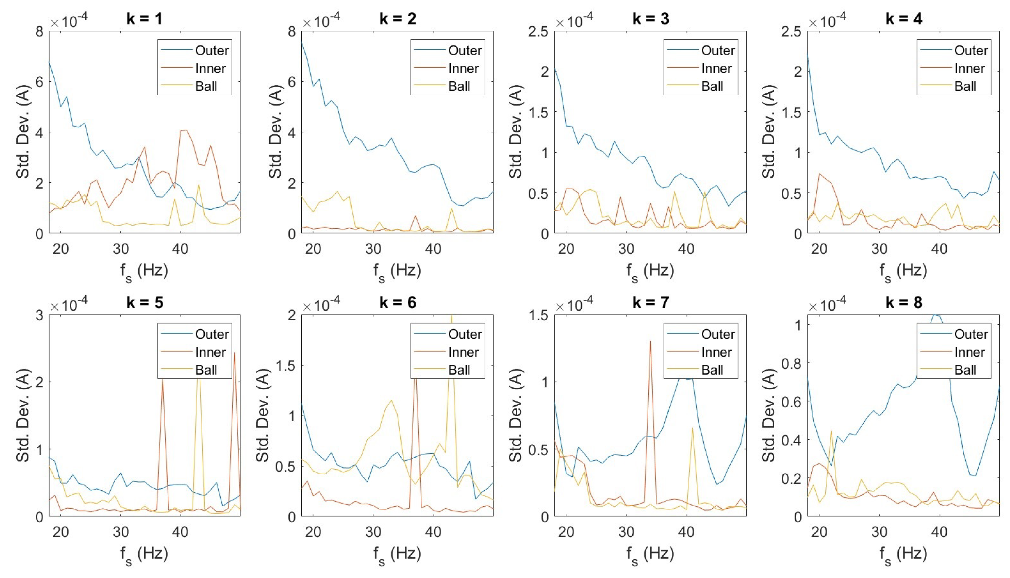
Although numerous other works have attempted to develop HIs that are independent of operating conditions, they exhibit several major limitations with respect to the objectives of this study. First, most state-of-the-art methods are developed and validated using vibration measurements. This is fundamentally different from motor current signature analysis (MCSA) because vibration signals generally have a higher signal-to-noise (S/N) ratio, which makes degradation trends more apparent and relatively easier to model. Second, the amplitude of vibration-based features tends to increase with rotational speed, which can be physically explained by the proportional relationship between acceleration, displacement, and the square of rotational speed. This direct relationship also reflects the relatively simple energy transmission path from the fault source to the vibration sensor. In contrast, the MCSA signal exhibits a lower S/N ratio, making it far more susceptible to noise. The signal propagation path in induction machines (IMs) is inherently more complex, involving multiple interacting electromagnetic and mechanical effects. Moreover, the overall trend of fault-related components in the current spectrum typically decreases with increasing speed, which is the opposite of what is observed in vibration-based analyses (as demonstrated later in this paper). These complexities make it challenging to design and implement condition monitoring algorithms for induction machines, which explains the comparatively limited progress in MCSA-based bearing fault diagnostics.

This gap highlights the need for a health indicator that remains independent of operating conditions—particularly the supply frequency—while still accurately reflecting the true degradation state of the bearing. Because the fault propagation path in induction machines is complex, a data-driven approach based on experimental measurements is adopted to compensate for the influence of supply frequency on the developed health indicator. However, data-driven methods alone do not reveal the underlying causality; i.e., which physical mechanisms are responsible for the trends observed in the experiments. To address this, a brief analysis of the key physical phenomena in induction machines is provided to support and interpret the experimental findings. This analysis explains how these mechanisms affect the detectability of bearing fault signatures in MCSA and establishes the expected trend of fault-related spectral components with respect to supply frequency. The predicted trend is subsequently verified through experimental data, which also forms the basis for implementing the proposed data-driven compensation approach.

Accordingly, Section 2 presents a theoretical background on how different effects in IM influence the detectability of bearing fault signatures and concludes with the expected trends of fault-related components with increasing supply frequency. Section 3 describes the experimental setup and validates these trends experimentally using two bearings with different fault severities. Based on the experimental data and observed trend, Section 4 details the construction of a regression-based model designed to stabilize the health indicator and proposes an alternative framework for model training, testing, and validation. Finally, Section 5 summarizes the key conclusions and contributions of this study.

2. Influence of Supply Frequency on Bearing Fault Signatures: Theoretical Background

This section provides a brief explanation behind the potential impact of supply frequency on the signature present in the stator current. The goal is to assess major phenomena and understand their potential contribution to health indicators based on the quantification of the bearing fault signature present in the stator current. Variations in the supply frequency can significantly influence the bearing fault frequencies in the current through both direct and indirect mechanisms. Several contributing factors may affect the manifestation of bearing fault signatures within the stator current frequency spectrum as a result of these frequency variations. The following are the main factors.

Changes in the supply frequency ($f_s$) directly influence the rotational frequency of the induction machine as the synchronous speed of the rotating magnetic field scales proportionally with $f_s$. Under load, the rotor operates below synchronous speed, and the resulting slip $s=(f_s-f_r)/f_s$ typically lies between 0.5–6%, as reported by Amitabh et al. [20]. Thus, increases in $f_s$ produce corresponding increases in shaft rotational frequency. Since bearing fault frequencies depend directly on shaft speed, as explained by Crowe [34], the characteristic components appear in the stator current at

$$f_{bf}=\mid f_s\pm n{f}_c\mid \mathrm{where}n=1,2,3,\dots$$

(1)

meaning that their spectral locations shift towards a higher frequency regime with increasing $f_s$, consistent with the observations of Jalonen et al. [35] and Huang et al. [36].

Although this spectral shift is straightforward, the amplitude of the bearing fault signature is strongly affected by both electrical and mechanical phenomena. Because bearing-fault sidebands have a comparatively low signal-to-noise ratio (SNR), as noted by Amitabh et al. [37], these influences become particularly significant.

On the electrical side, frequency-dependent effects—including impedance, the skin effect, and eddy currents—play a dominant role. The skin effect forces current toward conductor surfaces at higher frequencies, increasing the effective AC resistance according to Wheeler [38]:

$$R_{AC}=R_0\left(1+k_s\sqrt{{\displaystyle \frac{f}{f_0}}}\right).$$

(2)

Eddy currents, governed by Faraday’s law, also intensify with frequency, introducing magnetic damping that reduces the amplitude of current modulations associated with bearing faults, as shown by Gyselinck et al. [39] and Bellini et al. [40]. Reduced penetration depth further strengthens this attenuation, as demonstrated by Hamzehbahmani et al. [41]. These currents modify flux linkage in both stator and rotor circuits, as discussed by Ranta et al. [42,43] and Sudhoff et al. [44], and they appear explicitly in the standard voltage equations of the induction machine developed by Hütter et al. [45], Ranta and Arkkio [46], and Stoicuta [47]. Together with the natural increase in reactance ($j{\omega }_{s}L$), these effects increase the equivalent impedance experienced by higher-frequency components. Therefore, bearing fault harmonics—which shift to higher frequencies as $f_s$ increases—experience stronger attenuation, in line with classical electromagnetic theory [48,49,50,51,52].

On the mechanical side, rotor eccentricity and the resulting modulation strength depend on hydrodynamic bearing forces, unbalanced magnetic pull (UMP), centrifugal forces, and gyroscopic effects. Bearing faults introduce air-gap asymmetry that generates UMP, which can be expressed as in Zhu et al. [53] and Chen [54]:

$$F_{UMP}=\beta \pi DL{\left({\displaystyle \frac{B}{5000}}\right)}^2{\displaystyle \frac{e}{g_0}}.$$

(3)

Because the air-gap flux density decreases with frequency [55,56], the UMP stiffness scales as $k_{\mathrm{UMP}}\propto 1/f_s^2$, as shown by Jiang et al. [57], implying a rapid reduction in destabilizing force at higher $f_s$. In contrast, hydrodynamic film stiffness increases with rotational speed following

$$k_{\mathrm{dyn}};\approx ;C_{\mathrm{hb}},{\displaystyle \frac{\mu LR,\omega }{h^2}},$$

(4)

as given, for example, by Pinkus and Sternlicht [58], Hamrock et al. [59], and Childs [60], providing a stabilizing effect consistent with classical rotor–bearing dynamics described by Lund [61] and by Gunter and Barrett [62]. Centrifugal forces are negligible due to high shaft stiffness, and gyroscopic effects become important only near the critical speed, as reported by Wang and Han [63], Werner [64], and Shravankumar and Tiwari [65]. Combining these factors yields an equivalent stiffness for lateral motion of the shaft, which can be given as

$$k_{eq}=k-k_{UMP}\left({\omega }_s\right)+k_{dyn}\left({\omega }_s\right).$$

(5)

At low $f_s$, the large UMP and small hydrodynamic stiffness reduce $k_{\mathrm{eq}}$, allowing greater eccentric motion. As $f_s$ increases, $k_{\mathrm{UMP}}$ decreases sharply and $k_{\mathrm{dyn}}$ grows, increasing $k_{\mathrm{eq}}$ and suppressing radial displacement. Since the fault signature amplitude is proportional to this displacement, its magnitude decreases with increasing supply frequency. Additionally, the fault interaction time decreases at higher speeds because the rolling element traverses the defect more quickly, further reducing the excitation amplitude.

In summary, the amplitude of eccentric rotor motion decreases as the supply frequency increases. This mechanical effect is further reinforced by the electrical behavior of the machine, which shifts the bearing fault-related frequency components toward higher frequencies, thereby reducing their contribution in the lower-frequency region of the current spectrum. Consequently, a nonlinear decreasing trend is expected in the quantified bearing fault signature as the supply frequency rises.

It is important to emphasize that the objective of this section is to provide a conceptual explanation for the expected or observed trend and to illustrate the underlying mechanisms influencing the bearing fault signature, rather than to develop a complete simulation model. Although a full analytical representation of these phenomena is theoretically feasible for an induction machine, such modeling would require the integration of several complex equations along with numerous parameter assumptions and estimations. These uncertainties could significantly compromise the accuracy of the resulting model.

For these reasons, detailed simulations are considered beyond the scope of the present study. Instead, experimental validation is employed to capture the practical behavior. Based on the theoretical considerations outlined above, the overall expected response is a nonlinear decrease in the amplitude of the bearing fault signature within the current spectrum as the supply frequency increases.

3. Experiment and Validation

3.1. Test Setup and Experiments

For the experimental analysis, two bearings with different outer-race fault severities were tested using a squirrel-cage induction machine (model 3SIE100L4A, 2.2 kW, Cantoni Group, Cieszyn, Poland), as shown in Figure 1. The test bench consists of two coupled motors, where one machine operates as the test motor while the other provides the mechanical load. The test motor was disassembled to identify the bearing type installed on the shaft and to measure the air-gap clearance. The original bearings (6206 C3, SKF, Shanghai, China), equipped with riveted steel cages, were not suitable for the introduction of artificial defects due to the difficulty of disassembly. Consequently, an alternative bearing type (6206 TN9, SKF, Shanghai, China), featuring a nylon cage, was selected because it allows easier disassembly and facilitates the controlled introduction of outer-raceway faults.

Artificial defects were introduced on the outer raceway using carbide drill bits, which are among the hardest commercially available tools. Since the hardness of carbide is comparable to that of the bearing outer ring, significant tool wear occurred, necessitating the use of multiple drill bits throughout the process. The defects were machined radially, producing semicircular cross-sectional cavities extending across the entire raceway. Coherent holes were created to represent more severe fault conditions. Although such extensive damage is unlikely to occur in practical applications, these defects emulate scenarios in which multiple rolling elements simultaneously interact with a large eroded region of the outer raceway. The notation $3R1$ refers to three coherent holes of 1 mm radius, whereas $2R3$ designates two coherent holes of 3 mm radius, as illustrated in Figure 2. The tested machine exhibits steep torque–slip characteristics, implying that even small variations in slip are sufficient to produce substantial changes in torque.

The test bearings were mounted at the driving end of the motor and examined across 33 discrete rotational speeds, spanning from 500 to 1500 rpm. At each operating point, measurements were acquired for a duration of 5 min at a sampling frequency of 25.6 kHz using a National Instruments data acquisition system (25.6 kHz, 24-bit, ±5 V). Stator current signals were captured using three in-house-developed current sensors positioned on the phase conductors.

The rationale behind this measurement setup was to eliminate any preprocessing stages involving semiconductor-based electronics, which can introduce additional noise into the acquired signals [37]. For this reason, the current probes were designed to be fully inductive and non-invasive, ensuring that the data acquisition system recorded raw analog signals without intermediate electronic conditioning.

3.2. Signal Processing and Validation

The corresponding fault-related signatures in the current spectrum were then identified and quantified to assess their progression. Following the methodology in [7], analysis focused on the sensitive frequency band surrounding the theoretically derived bearing fault frequencies and their harmonics (outer race, inner race, and ball defect), using the extracted supply and rotational frequencies from each measurement. A schematic representation of the quantification process for the sensitive frequency band is provided in Figure 3.

The first observation concerns the variation in the amplitude of the fundamental component. As shown in Figure 4, the amplitude of the fundamental component tends to decrease with increasing supply frequency. This behavior can be attributed to the combined effects of the skin effect and eddy currents, which increase the overall impedance and consequently reduce the current amplitude for a fixed supply voltage. However, the overall impact remains modest, with a variation of approximately 200 mA. In contrast, the variation is more pronounced for the bearing fault signatures observed in the current spectrum.

The acquired current signals were processed using the signal processing methodology described in [7]. The sensitive frequency bands were then quantified, and Figure 5 presents the mean values up to the 4th harmonic. According to Equation (1), each value of n corresponds to two distinct frequencies associated with the bearing fault signature. Consequently, each n produces two values of k in Figure 5, denoted as $k=2n-1$ and $k=2n$.

It can be observed that the overall magnitude of the bearing fault signatures decreases with increasing supply frequency. For $k=1$, this trend is more pronounced compared to higher-order values such as $k=8$, since most of the signal energy is concentrated in the lower harmonics rather than the higher ones. This is evident in Figure 5, where the mean values of the data points are consistently larger for lower values of k. Conversely, for higher-order terms, particularly $k=7$ and $k=8$, the trend becomes less distinct due to the reduced signal-to-noise ratio at higher frequencies, where noise contributions become more dominant.

Additionally, for $k=7$ and $k=8$, a localized rising trend is visible around the supply frequency of 40 Hz. This behavior can be attributed to interference effects arising from the supply frequency or its harmonics, as well as from the rotational frequency. A similar trend is observed when evaluating the standard deviation of the data points within each sensitive frequency band, as illustrated in Figure 6.

The trend is more prominent for lower values of k but diminishes progressively at higher values. An additional observation is the re-emergence of an increasing trend near the supply frequency of 50 Hz, particularly for higher-order values of k. This behavior can be attributed to spectral spreading (also referred to as frequency smearing in the literature [66]).

Spectral spreading occurs in the Fourier transform when a given frequency component is not strictly constant within the signal but exhibits small variations during the measurement period [67]. In inverter-fed machines, the supply frequency is not perfectly stable and undergoes slight fluctuations over time. These variations also affect the rotational frequency, which prevents the bearing fault frequencies from appearing as sharp peaks. Instead, the spectral energy is distributed over a small band, producing a “smeared” patch rather than a distinct line.

However, as the machine supply frequency approaches the nominal inverter supply frequency (50 Hz), the inverter delivers a cleaner voltage signal. This reduces the frequency smearing effect, allowing the bearing fault signatures to appear as sharper peaks, which is reflected in the increased standard deviation observed around 50 Hz. While this effect is negligible for dominant components with a high signal-to-noise ratio, it becomes significant for weaker components with low signal-to-noise ratios. Consequently, this trend is particularly evident at higher harmonics associated with the bearing fault frequencies and can be observed in both the mean and standard deviation plots.

Hence, it can be concluded that the observed decreasing trend in amplitude supports the formulated theory presented in Section 2. However, a direct validation for each element discussed in Section 2 through experimental measurements would require an extensive campaign with a more complex test setup, which lies beyond the scope of this work and may be considered for future investigations. Consequently, relying solely on the amplitude of the current signature as a health indicator may result in false diagnoses and inaccurate severity estimation in the presence of speed variations. This highlights the need for additional efforts to develop a speed-independent health indicator.

4. Supply Frequency Compensation

In industrial applications, machines are generally not expected to operate at a single operating speed but often vary operation between different steady-state speed settings. As discussed in the previous section, the health indicator (HI) exhibits significant variation under different operating speeds. Consequently, relying directly on the HI to estimate the remaining useful life (RUL) introduces considerable uncertainty. This highlights the necessity of developing a methodology capable of minimizing or eliminating the influence of operating speed on the signal amplitude. In this paper, the goal is to ensure an HI which is independent of speed variations.

In this study, a data-driven approach is adopted because estimating the underlying physical parameters is highly complex, involves multiple degrees of freedom, and is therefore beyond the scope of this work. Although several regression-based machine learning techniques—such as neural networks, LSTMs, and CNNs—could be employed to compensate for the influence of supply frequency, a simple regression model is chosen to ensure computational efficiency [68,69]. While neural network architectures have greater capacity to capture complex nonlinear relationships, the experimentally observed trend in this case is relatively straightforward and does not exhibit the level of nonlinearity or interaction that would justify the use of more advanced models. Selecting a lightweight regression model is also advantageous for real-time condition-monitoring applications, where minimizing computational burden is essential.

Several studies in the literature have reported that the bearing fault signature in the current spectrum exhibits nonlinear variation with increasing eccentricity values [20,70]. In [71], the authors proposed a quadratic functional relationship, supported by analytical reasoning, to describe how the signature amplitude is affected. However, their model assumes that eccentricity is independent of the operating condition.

In the present case, it was observed that eccentricity is also a function of the supply frequency. This dependency necessitates the use of a higher-order functional representation to accurately capture the variation in the signal. Accordingly, a fifth-order polynomial is assumed to compensate for the effect of changes in supply frequency. The rationale for selecting a fifth-order expression is discussed in detail later in this section.

The health indicator (HI) is derived as a weighted combination of the mean and standard deviation, following the formulation presented in [7] and is given by Equation (6).

$$\mathrm{HI}={\displaystyle \frac{{\sum }_{k=1}^{k}w{t}_1\left(k\right)·STD\left(k\right)}{{\sum }_{k=1}^{k}w{t}_1\left(k\right)}}+10·{\displaystyle \frac{{\sum }_{k=1}^{k}w{t}_2\left(k\right)·Mean\left(k\right)}{{\sum }_{k=1}^{k}w{t}_2\left(k\right)}}$$

(6)

where the weights $w{t}_1$ and $w{t}_2$ are calculated using Equation (7)

$$w{t}_1\left(k\right)=a_1{e}^{-\frac{|k-c_1|}{b_1}}\mathrm{and}w{t}_2\left(k\right)=a_2{e}^{-\frac{k}{b_2}}$$

(7)

The weights has decreasing trend for mean and increasing trend for standard deviation. This is based on the observed trend reported in [7]. The values of $a_1$, $a_2$, $b_1$, $b_2$ and $c_1$ are chosen such that the values of $w{t}_1$ and $w{t}_2$ have a sufficient decay trend with respect to k, which is neither too flat nor too steep.

Ideally, the HI should exhibit invariance under varying operating conditions. To achieve this, a compensating function ($c\left(f\right)$) is introduced such that the product of the HI and ($c\left(f\right)$) results in a constant value $k_c$. In other words, $c\left(f\right)$ serves as an $f_s$-dependent gain factor applied to the health indicator, ensuring that the overall outcome remains constant across all operating supply frequencies. This ensures that the HI becomes independent of the supply frequency $f_s$ for a given faulty bearing (Equation (8)).

$$HI·c\left(f\right)=k_{c}ORHI·c\left(f\right)-k_c=0$$

(8)

where

$$c\left(f\right)=c_0+c_{1}f+c_2{f}^2+c_3{f}^3+c_4{f}^4+c_5{f}^5$$

(9)

It is important to note that the constant $k_c$ is also unknown. What is known, however, is that $k_c$ remains constant for a given bearing and its magnitude is expected to correlate with the severity of the damage; i.e., being higher for bearings with more severe faults and lower for those with less significant damage.

This formulation naturally leads to a regression problem, where the objective is to determine the optimal parameters by minimizing a cost function, as defined in Equation (10).

$$\underset{\left\{c_m\right\},\left\{k_c\right\}}{min}\sum _j{\left(H{I}_j\sum _{m=0}^5{c}_m{f}_j^m-k_c\right)}^2$$

(10)

Here, $H{I}_j$ denotes the health indicator calculated at the jth supply frequency. The reference frequency is chosen as $f_0=34$ Hz, which approximately corresponds to the midpoint of the frequency range used in the measurements (18–50 Hz). For this reference condition, the compensating function is normalized such that $c\left(f_0\right)=1$. This normalization ensures that the scale of the polynomial is fixed, thereby yielding a unique solution during model estimation. After performing the regression using the measurement data from bearing 3R1, the resulting polynomial coefficients are presented in

Table 1. Polynomial coefficients of the frequency (per unit) correction function $c\left(f\right)={\sum }_{m=0}^5{c}_m{f}^m$.

Coefficient	Value
$c_0$	$2.44265716\times {10}^{-5}$
$c_1$	$2.89367176\times {10}^{-4}$
$c_2$	$2.21345019\times {10}^{-3}$
$c_3$	$-3.04032787\times {10}^{-5}$
$c_4$	$-7.42508463\times {10}^{-7}$
$c_5$	$1.36149258\times {10}^{-8}$

.

The obtained coefficients are of relatively small magnitude, making it challenging to directly assess the relative dominance or contribution of each term in the polynomial. To facilitate a clearer comparison and improve interpretability, a per-unit (p.u.) normalization is applied to the frequency variable. Specifically, the frequency f is expressed in per-unit form by substituting $f=f/50$, where 50 Hz represents the nominal supply frequency. This normalization scales the frequency variable to a dimensionless range, thereby adjusting the numerical magnitude of the polynomial coefficients to a comparable level. The resulting normalized coefficients are presented in

Table 2. Polynomial coefficients of the frequency correction function $c\left(f\right)={\sum }_{m=0}^5{c}_m{f}^m$.

Coefficient	Value
$c_0$	$2.44265716\times {10}^{-5}$
$c_1$	$1.446835\times {10}^{-2}$
$c_2$	$5.5336$
$c_3$	$-3.8004$
$c_4$	$-4.6407$
$c_5$	$4.2547$

.

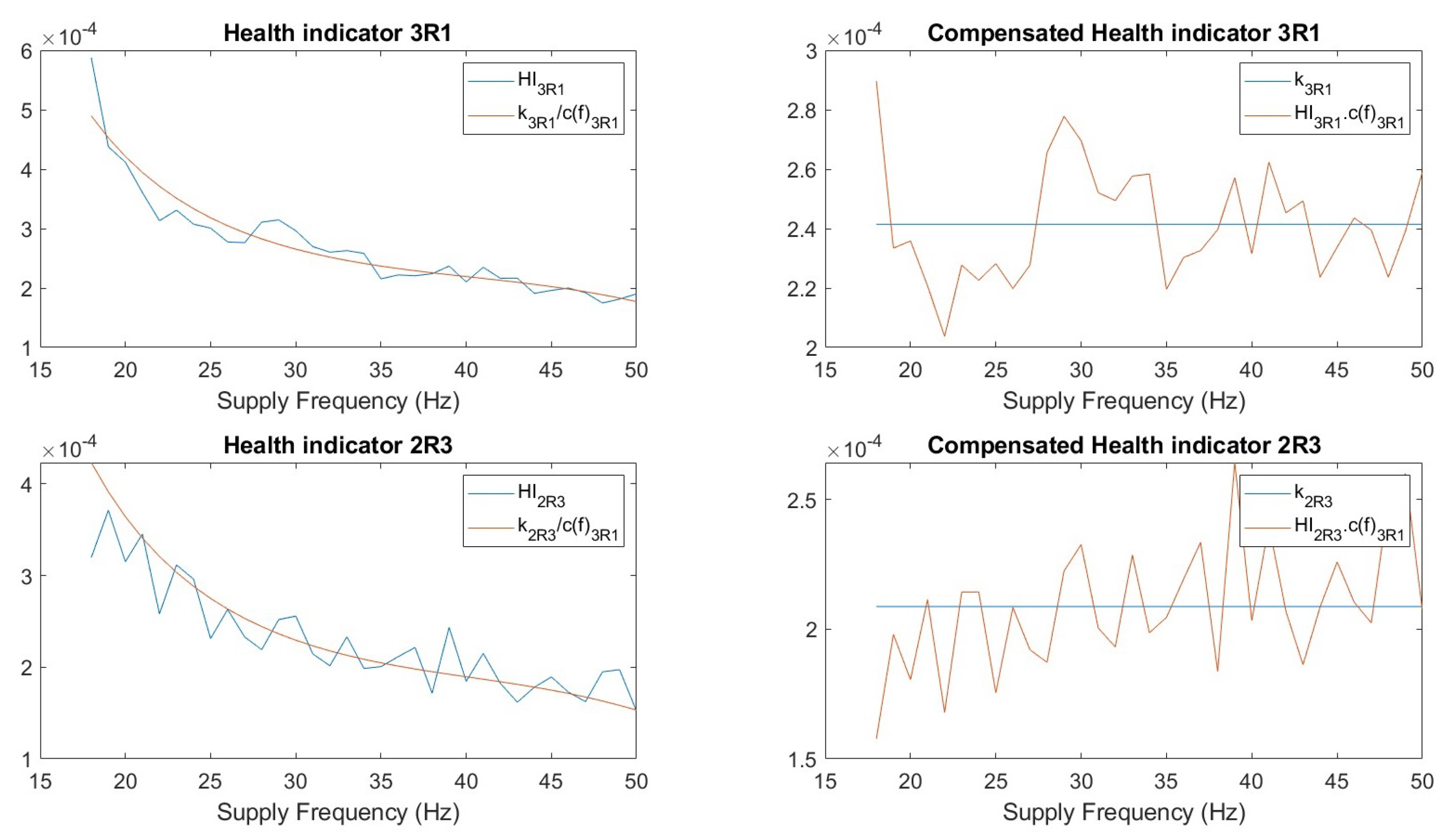
Using these coefficients and the health indicator calculated for each speed, we get

$$k_{3R1}=\mathrm{mean}(H{I}_{3R1}\left(f\right)·c\left(f\right))=2.4143\times {10}^{-4}$$

(11)

Similarly, for bearing 2R3

$$k_{2R3}=\mathrm{mean}(H{I}_{2R3}\left(f\right)·c\left(f\right))=2.0869\times {10}^{-4}$$

(12)

The overall regression response is illustrated in Figure 7. It can be observed that $k_{3R1}>k_{2R3}$, indicating that the frequency-independent health indicator has a higher value for the more severely damaged bearing. This trend is consistent with findings reported in the literature [7].

At lower operating frequencies, the contributions of the third-, fourth-, and fifth-order terms are minimal, making the second-order term the dominant component of the compensating function $c\left(f\right)$ such that it can be reasonably approximated as a quadratic function, sufficiently capturing the variation in the signal. However, as the supply frequency approaches the rated value of 50 Hz, the influence of the higher-order terms becomes increasingly significant. This shift in dominance indicates that $c\left(f\right)$ deviates from a purely quadratic form and instead exhibits higher-order nonlinear characteristics. This behavior is particularly relevant for practical applications, since electrical machines typically operate in the vicinity of their rated frequency, where such nonlinear effects are most pronounced. Furthermore, the zeroth- and first-order coefficients remain negligible across the entire frequency range, confirming that the overall response cannot be considered linear.

A common practice in training data-driven models is to use a mixed dataset that captures all possible operating scenarios and to divide it into training and testing subsets, typically in a 70:30 ratio, where 70% is used for training and 30% for validation and testing [72,73]. In the present case, this would imply that the training dataset includes data from both faulty bearings. Such an approach could lead the regression model to fit the dataset regardless of the order of the assumed polynomial, potentially resulting in overfitting, especially when higher-order equations are employed.

In this study, however, a different training strategy is adopted. The approach is based on the premise that the compensating function $c\left(f\right)$ represents the correction for supply frequency and should, in principle, remain independent of the bearing degradation level. Consequently, the coefficients of $c\left(f\right)$ are expected to be invariant, irrespective of which degradation level is used to train the model. This assumption provides a meaningful framework for evaluating and selecting the appropriate order of the regression model. If validated, it would also imply that data from a single faulty bearing could be sufficient to train a model capable of representing all degradation levels, thereby substantially reducing the amount of data required for training.

Previously, it can be seen that the regression model was trained using measurement data from bearing 3R1 and subsequently tested using data from bearing 2R3. However, at this stage, it is not possible to confirm whether the obtained coefficients correspond to an overfitted model. This uncertainty arises because both the training and validation datasets were derived exclusively from measurements of bearing 3R1. In other words, the algorithm had no prior exposure to the data corresponding to bearing 2R3. Consequently, no direct quantitative indicator is available to assess how accurately the model fits the measurements from bearing 2R3.

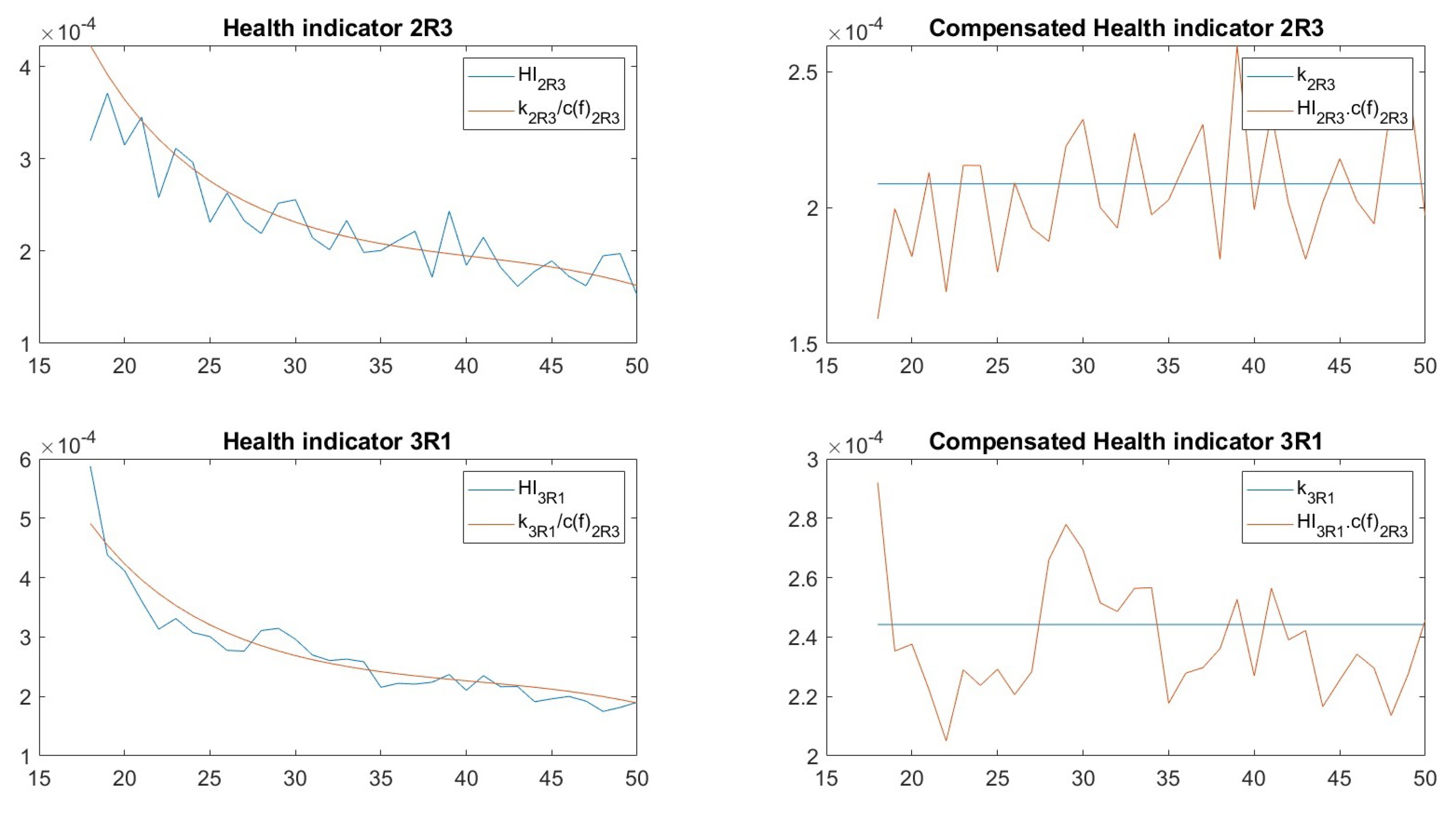
To address this, the procedure was repeated by interchanging the datasets—that is, training and validating the model using data from bearing 2R3, and testing it with data from bearing 3R1. The objective of this cross-validation approach is to evaluate the extent to which the estimated coefficients differ in the two cases. A significant deviation would suggest that either (i) the chosen functional form is inadequate to capture the underlying dynamics, or (ii) the model is overfitted to the training data.

Table 3. Comparison of 5th-order polynomial coefficients and constants between the original and reversed analyses.

Term	Original (3R1 as Ref)	Reversed (2R3 as Ref)	Percent Difference
$c_0$	$+2.4427\times {10}^{-5}$	$+2.5551\times {10}^{-5}$	$+4.6\%$
$c_1$	$+1.446835\times {10}^{-2}$	$+1.4842\times {10}^{-2}$	$+2.6\%$
$c_2$	$+5.5336$	$+5.5976$	$+1.2\%$
$c_3$	$-3.8004$	$-3.8615$	$+1.6\%$
$c_4$	$-4.6407$	$-4.7397$	$+2.1\%$
$c_5$	$+4.2547$	$+4.2810$	$+0.6\%$
$k_{3\mathrm{R}1}$	$2.4143\times {10}^{-4}$	$2.4421\times {10}^{-4}$	$+1.15\%$
$k_{2\mathrm{R}3}$	$2.0869\times {10}^{-4}$	$2.1035\times {10}^{-4}$	$+0.8\%$

summarizes the coefficients obtained from both methods and presents the corresponding percentage differences, while Figure 8 illustrates the regression response with two datasets being used in the reverse order.

A similar analysis was performed for various polynomial orders, ranging from a second-order to an eighth-order expression for $c\left(f\right)$. The objective of this exercise was to determine the polynomial order for which the percentage difference between the coefficients is minimum. Since the compensating function $c\left(f\right)$ is expected to remain valid across different levels of bearing severity, the corresponding coefficients should ideally remain consistent regardless of the dataset used for training.

Table A1. Comparison of 2nd-order polynomial coefficients and constants for both bearings.

Term	Original (3R1 as Ref)	Reversed (2R3 as Ref)	Percent Difference
$c_0$	$-3.909\times {10}^{-1}$	$-1.637\times {10}^{-1}$	$-58.1\%$
$c_1$	$+2.8915$	$+2.4830$	$-14.1\%$
$c_2$	$-1.2443$	$-1.1350$	$-8.8\%$
$k_{3\mathrm{R}1}$	$2.398\times {10}^{-4}$	$2.446\times {10}^{-4}$	$+2.0\%$
$k_{2\mathrm{R}3}$	$2.073\times {10}^{-4}$	$2.106\times {10}^{-4}$	$+1.6\%$

,

Table A2. Comparison of 3rd-order polynomial coefficients and constants for both bearings.

Term	Original (3R1 as Ref)	Reversed (2R3 as Ref)	Percent Difference
$c_0$	$-1.804$	$-3.124\times {10}^{-1}$	$-82.7\%$
$c_1$	$10.27$	$3.2380$	$-68.5\%$
$c_2$	$-13.21$	$-2.3338$	$-82.3\%$
$c_3$	$+6.1388$	$+0.6036$	$-90.2\%$
$k_{3\mathrm{R}1}$	$2.449\times {10}^{-4}$	$2.441\times {10}^{-4}$	$-0.3\%$
$k_{2\mathrm{R}3}$	$2.119\times {10}^{-4}$	$2.109\times {10}^{-4}$	$-0.5\%$

,

Table A3. Comparison of 4th-order polynomial coefficients and constants for both bearings.

Term	Original (3R1 as Ref)	Reversed (2R3 as Ref)	Percent Difference
$c_0$	$-8.627\times {10}^{-1}$	$-2.033\times {10}^{-1}$	$-76.4\%$
$c_1$	$+5.075$	$+2.8405$	$-44.0\%$
$c_2$	$-7.5375$	$-3.1900$	$-57.7\%$
$c_3$	$+4.0125$	$+1.9025$	$-52.6\%$
$c_4$	$-0.6756$	$-0.3236$	$-52.1\%$
$k_{3\mathrm{R}1}$	$2.417\times {10}^{-4}$	$2.444\times {10}^{-4}$	$+1.1\%$
$k_{2\mathrm{R}3}$	$2.095\times {10}^{-4}$	$2.103\times {10}^{-4}$	$+0.4\%$

,

Table A4. Comparison of 6th-order polynomial coefficients and constants for both bearings.

Term	Original (3R1 as Ref)	Reversed (2R3 as Ref)	Percent Difference
$c_0$	$-4.292\times {10}^{-2}$	$-3.044\times {10}^{-2}$	$-29.1\%$
$c_1$	$+0.7255$	$+0.6025$	$-17.0\%$
$c_2$	$-4.7950$	$-4.325$	$-9.2\%$
$c_3$	$+13.8125$	$+13.4125$	$-2.9\%$
$c_4$	$-19.1875$	$-19.3188$	$+2.2\%$
$c_5$	$+12.5$	$+13.0031$	$+4.0\%$
$c_6$	$-3.0609$	$-3.2703$	$+6.8\%$
$k_{3\mathrm{R}1}$	$2.455\times {10}^{-4}$	$2.460\times {10}^{-4}$	$+0.2\%$
$k_{2\mathrm{R}3}$	$2.120\times {10}^{-4}$	$2.117\times {10}^{-4}$	$-0.1\%$

,

Table A5. Comparison of 7th-order polynomial coefficients and constants (unstable solution).

Term	Original (3R1 as Ref)	Reversed (2R3 as Ref)	Percent Difference
$c_0$	$+1.364\times {10}^3$	$+9.028\times {10}^2$	$-33.8\%$
$c_1$	$-1.4565\times {10}^4$	$-9.69\times {10}^3$	$-33.5\%$
$c_2$	$+6.1925\times {10}^4$	$+4.0125\times {10}^4$	$-35.2\%$
$c_3$	$-1.3275\times {10}^5$	$-8.349\times {10}^4$	$-37.1\%$
$c_4$	$+1.5356\times {10}^5$	$+9.237\times {10}^4$	$-39.9\%$
$c_5$	$-9.4156\times {10}^4$	$-5.4875\times {10}^4$	$-41.7\%$
$c_6$	$+2.841\times {10}^4$	$+1.6625\times {10}^4$	$-41.9\%$
$c_7$	$-3.3781\times {10}^3$	$-1.9609\times {10}^3$	$-41.9\%$
$k_{3\mathrm{R}1}$	$3.863\times {10}^{-6}$	$4.937\times {10}^{-6}$	$+27.8\%$
$k_{2\mathrm{R}3}$	$6.900\times {10}^{-5}$	$7.800\times {10}^{-5}$	$+13.0\%$

and

Table A6. Comparison of 8th-order polynomial coefficients and constants (divergent solution).

Term	Original (3R1 as Ref)	Reversed (2R3 as Ref)	Percent Difference
$c_0$	$-1.909\times {10}^{-13}$	$-1.105\times {10}^{-13}$	$-42.1\%$
$c_1$	$-1.884\times {10}^{-10}$	$-1.090\times {10}^{-10}$	$-42.1\%$
$c_2$	$-1.749\times {10}^{-7}$	$-1.001\times {10}^{-7}$	$-42.8\%$
$c_3$	$-5.966\times {10}^{-5}$	$-3.290\times {10}^{-5}$	$-43.3\%$
$c_4$	$+2.211\times {10}^{-1}$	$+1.64\times {10}^{-2}$	$-92.6\%$
$c_5$	$-4.05\times {10}^1$	$-2.24\times {10}^1$	$-44.7\%$
$c_6$	$+2.8671\times {10}^2$	$+2.2609\times {10}^2$	$-21.1\%$
$c_7$	$-4.754\times {10}^2$	$-4.095\times {10}^2$	$-13.9\%$
$c_8$	$+2.2964\times {10}^2$	$+2.0625\times {10}^2$	$-10.2\%$
$k_{3\mathrm{R}1}$	$2.840\times {10}^{-9}$	$1.162\times {10}^{-9}$	$-59.1\%$
$k_{2\mathrm{R}3}$	$9.410\times {10}^{-5}$	$1.902\times {10}^{-4}$	$+102.1\%$

in Appendix A and Table 3 summarize the percentage deviations in the coefficients obtained for each assumed polynomial order. It can be observed that the fifth-order equation yields the smallest difference between the coefficients estimated using bearing 3R1 as the reference and those estimated using bearing 2R3 as the reference. This consistency indicates that the selected fifth-order form of $c\left(f\right)$ is not overfitted and is sufficiently flexible to represent the compensating behavior across different damage severities. Therefore, the fifth-order polynomial is considered the most appropriate choice for modeling the compensating factor.

It is also observed that the deviations between the predicted and measured values are relatively higher, primarily due to the limited size of the training dataset. The accuracy of the regression model is expected to improve if a time-averaged health indicator is employed instead of relying on single-measurement values. Moreover, increasing the number of operating speeds included in the training phase would likely enhance the robustness of the model and reduce the observed discrepancies.

The regression approach proposed above represents one possible methodology for compensating for the influence of $f_s$ on the health indicator (HI). Nevertheless, more advanced data-driven techniques—such as regression-based neural networks—could also be investigated, as they possess the capability to model nonlinear relationships more effectively. Despite this, the overall outcome is expected to remain comparable, given that the available training data exhibit a monotonic decreasing trend. Therefore, based on the current dataset, it can be concluded that a simpler regression-based approach is adequate for accurately capturing the underlying trend while maintaining a low computational cost.

It should be noted that the proposed methodology has been validated only for the set of measurements presented in this paper. The approach can be considered fully generalizable only if the compensating function $c\left(f\right)$ demonstrates consistent performance across a wider range of bearing fault severities and different machine types. Achieving this will require the collection of additional experimental data.

From an implementation standpoint, the compensating function $c\left(f\right)$ can be readily integrated into a practical machine monitoring system. Instead of requiring a large dataset obtained from multiple bearings at various degradation levels, the regression model can be effectively trained using data from only two or three bearings representing different health conditions. It is important to note, however, that the coefficients presented in this study are machine-specific, as they depend on the design and operating characteristics of the particular system. Consequently, independent measurements are required when applying this model to other machines. Moreover, the coefficients may vary over time due to machine aging or component wear, necessitating the use of adaptation routines to periodically update the model parameters. Here, the adaptation routine refers to an algorithmic process that periodically re-establishes or adjusts the input–output mapping of a model based on newly acquired operational data, ensuring that the model remains representative of the system’s current state. The interesting fact here is that such an adaptation routine does not account for changes in system behavior caused by varying degradation levels; therefore, performing this routine preserves the model’s validity specifically with respect to bearing fault estimation. These adaptive mechanisms are widely employed in condition monitoring and control applications where gradual aging or wear affects system dynamics, such as in transmission clutches, hydraulic pumps, and rotating machinery [74,75].

At this stage, the health indicator (HI) is rendered independent of the supply frequency, thereby ensuring that it provides a consistent and stable value corresponding to a specific level of bearing degradation. Nevertheless, it is imperative to establish a reference threshold for the HI that represents the state of complete degradation (i.e., 100% degradation) of the bearing. The determination of this reference point is inherently system-dependent, as it is influenced by the operational characteristics and design configuration of the system in which the bearing is integrated.

In general, bearing degradation affects several interconnected phenomena such as vibration intensity, acoustic noise emission, and variations within the magnetic circuit. These effects, in turn, may compromise the structural integrity of the system, contribute to environmental noise pollution, and potentially induce undesirable resonance in the electrical subsystem. The extent to which these consequences are considered detrimental varies across applications; hence, the definition of a 100% degradation level must be tailored to the specific operational environment.

Accordingly, a one-time calibration or mapping procedure is required for each application to establish this system-specific reference. During this process, multiple system responses—including vibration amplitude, noise level, and magnetic circuit fluctuations—should be continuously monitored. Based on these observations, the user or system designer can determine the maximum permissible bearing degradation that can be tolerated without adversely affecting the performance or reliability of adjacent components or subsystems.

In summary, three bearings can be considered sufficient to establish a baseline for estimating degradation severity in percentage terms. Two bearings exhibiting moderate levels of fault (between 0% and 100% degradation) can be utilized to determine the $c\left(f\right)$ coefficients, while one bearing with the highest acceptable severity level can be used to map the HI corresponding to 100% degradation. In this manner, the proposed methodology can be extended such that the HI provides a direct quantitative indication of degradation in terms of percentage.

5. Conclusions

This paper advances the field of condition monitoring by analyzing how various electrical and mechanical factors influence the amplitude of bearing fault signatures in the current spectrum, enabling the development of a supply-frequency-independent health indicator. Subsequently, a data-driven methodology was proposed to compensate for the net impact of supply frequency, thereby stabilizing the health indicator (HI) over different operating speeds and improving diagnostic reliability.

Initially, the impact of major factors were assessed on the bearing fault signatures in the current spectrum. Analytical evaluation revealed that most of these factors exhibit a nonlinear attenuating influence on the fault signature amplitude. As the supply frequency ($f_s$) increases, mechanical effects tend to oppose the eccentric motion of the rotor, while electrical effects further attenuate the higher-frequency components in the signal.

Because analytically isolating the influence of each individual factor is not feasible with the current setup, experimental validation was conducted using two faulty bearings tested across multiple rotational speeds to observe the collective effect of all contributing elements. The results confirmed that the amplitude of the bearing fault signatures decreases nonlinearly as the supply frequency increases.

Such attenuation can lead to inaccurate assessments of fault severity and, consequently, erroneous estimation of the remaining useful life (RUL). Therefore, compensating for the influence of supply frequency is crucial. In this study, a regression-based model was employed to achieve this compensation, selected for its simplicity and computational efficiency. The validation approach was based on the principle that a model trained on one bearing should perform effectively on another, implying minimal variation in model coefficients between the two cases; specifically, (a) training on 3R1 and testing on 2R3, and (b) vice versa. The fifth-order compensation function, $c\left(f\right)$, demonstrated the best performance and was thus adopted. After applying the compensation, the health indicator exhibited a nearly constant trend across different supply frequencies, confirming the effectiveness of the proposed method.

The novelty of this work lies in developing a modified regression-based approach to construct a speed- or frequency-independent health indicator. The proposed compensating factor, $c\left(f\right)$, is derived directly from the physical understanding established in Section 2. It is designed to effectively counteract the influence of supply frequency on the health indicator, making it applicable to bearings with different damage severities. In essence, the coefficients of $c\left(f\right)$ should capture the general variation in supply frequency common to all faulty bearings, differing only by an offset determined by the fault severity. The validity of this assumption was confirmed through experimental analysis, showing that the regression coefficients exhibit minimal variation across bearings.

A key advantage of this approach is its modest data requirement. As shown, measurements from only a few faulty bearings are sufficient to determine $c\left(f\right)$ and establish acceptable degradation thresholds. Furthermore, regression models are computationally efficient compared to more complex architectures such as neural networks. Thus, the combined effort—limited data acquisition and low-complexity model development—makes this technique practical for deployment in real industrial environments.

However, the principal limitation of the proposed method is that it remains data-driven and does not fully capture the causal mechanisms governing the system. Incorporating deeper mechanistic understanding would require independently evaluating each factor discussed in Section 2, which in turn demands a more sophisticated test setup and substantially greater experimental effort. An alternative pathway is the development of a high-fidelity physical model that integrates these phenomena, enabling the construction of a digital twin capable of accurately representing machine behavior under varying operating conditions. Such an approach would increase physical interpretability while reducing reliance on data-driven assumptions. Moreover, although the proposed regression model demonstrates strong performance with limited data, a more extensive validation campaign—using a larger and more diverse dataset spanning a wider range of fault severities—is necessary to further strengthen confidence in the methodology. These limitations provide clear directions for future work.

Overall, this study provides both a theoretical foundation for understanding frequency-dependent effects in induction machines and a practical, low-complexity regression-based framework to compensate for them. The combination of physical interpretability, computational efficiency, and reduced data requirements represents a significant step toward developing robust, frequency-independent health indicators for induction machine condition monitoring.