Steering Accuracy Analysis of Cam Mechanism in Complex Trajectory Based on Return Error of Gear Transmission

Abstract

The trajectory accuracy of equipment with complex motion paths presents a critical engineering challenge. Targeting the precision issues in the operating trajectory of a carbon-free car, this paper proposes an optimization method for complex mechanical trajectories. Firstly, this study investigates gear backlash-induced return error on the steering precision of a carbon-free cam mechanism of cars. Secondly, considering the cumulative return error of gear transmission between gear groups, a comprehensive mathematical model was established to guide the optimization of cam structure. Finally, the steering accuracy before and after optimization is quantitatively evaluated by trajectory calculation. In addition, the optimized structure was tested and compared with the numerical calculation. The experimental and numerical calculation results are highly consistent. The numerical calculation results show that by adjusting the transmission ratio of the gear set and optimizing the cam profile, the cam deflection angle error is reduced by 24.74% and 27.15%, respectively, and the comprehensive cumulative deflection error of the car is significantly reduced by 45.31%. More importantly, the research provides crucial technical support and guidance for achieving precise control and planning complex paths in automated production lines.

1. Introduction

In recent years, the machining of complex trajectories and the prediction of complex paths have become one of the critical challenges in engineering applications [1,2,3,4,5,6]. This paper takes the carbon-free car [7,8,9] with intricate travel paths as the research object and investigates methods for optimizing its trajectory. The cam of the carbon-free car’s steering mechanism [10] is an important mechanism that affects the accuracy and stability of the carbon-free car’s running trajectory. It has the advantages of simple structure, compactness, and controllable action law [11,12]. Therefore, it is of great significance to study the influence of cam processing and assembly error on the trajectory accuracy of a carbon-free car, which is of great significance to the design and optimization of the car.

The cam mechanism is the decisive factor for the steering system of the carbon-free car. Many scholars have studied the design of the cam mechanism. Iriarte et al. [13] and Zhou et al. [14] proposed different designs and analysis methods for cam mechanisms, respectively. Previous results show that the cam trajectory designed by the proposed method is more accurate. The experimental results demonstrate that the proposed method effectively mitigates vibrations in the cam mechanism, resulting in a lower impact velocity. Pozo-Palacios et al. [15] evaluated forward and inverse cam synthesis methods for designing a multi-leaf cam rocker-slider mechanism. The results show that the torque ripple of the cam designed by the reverse method is reduced by at least 50.97%. Lan et al. [16] attributed design flaws in cam transmission mechanisms to geometric imperfections and consequently developed a defect recognition algorithm. Numerical simulations subsequently validated the algorithm’s feasibility. Yang et al. [17] introduced a design for a novel coaxial indexing mechanism based on a conjugate cam and a parallelogram linkage. To this end, they constructed a prototype and conducted physical experiments. The results show that the cam mechanism designed by this method is more compact and the transmission effect is better. Zheng et al. [18] designed a solar truck with a single cam as the steering guide mechanism, established a dynamic model of the car, and carried out numerical calculations. The results show that the single cam steering structure exhibits excellent mechanical properties and an accurate trajectory. In addition, some scholars have also carried out optimization research on cam design. Wang and Peng [19] applied an Improved Hunter–Prey Optimization (IHPO) algorithm to optimize the sizing parameters of an oscillating follower cam mechanism. These results demonstrate the method’s efficacy in enhancing the motion reliability of disk cam mechanisms, offering valuable insights for broader cam design applications. Zhu et al. [20] developed a parameter optimization method for designing and analyzing large-scale, high-speed cam-linkage mechanisms, taking into account motion performance. They validated their approach through its successful application to a lateral device. The optimization results show that the productivity of horizontal equipment has doubled. Kang et al. [21] addressed the optimization and dynamic analysis of a spring-driven cam-linkage mechanism in vacuum circuit breakers, demonstrating that their optimized design significantly reduces the Hertz stress at the cam follower interface. While these studies primarily focus on cam design methodologies, they have overlooked the influence of gear backlash on transmission accuracy.

Gear backlash, which is an inherent characteristic of the transmission system, constitutes the critical factor influencing the positioning precision of cam steering mechanisms [22]; some scholars have studied gear backlash. By establishing a thermal backlash model for a planetary gear system, Wang et al. [23] analyzed its nonlinear dynamic characteristics and demonstrated that temperature plays an important role in backlash variation. Tian et al. [24] investigated the coupled dynamics of gear backlash and bearing clearance, uncovering a range of rich nonlinear phenomena. Zenn et al. [25] and Reddy et al. [26] proposed methods of measuring the gear gap size, respectively, both of which can accurately estimate the gear gap size. The above studies do not consider the influence of backlash-induced return error of gear transmission on the steering accuracy of the cam follower mechanism. This negligence will lead to the deviation between the actual cam angle and the theoretical value, thus affecting the cam steering accuracy.

In summary, this paper examines the effect of gear transmission backlash error on the steering accuracy of cam mechanisms in a carbon-neutral car. Firstly, we develop a mathematical model for the return error of gear transmission in gear transmission and propose optimization methods. Secondly, computational analyses are performed using MATLAB 2023b to derive simulated trajectories, which are then compared with theoretical trajectories to assess the impact of the return error of gear transmission on the precision of car operation. Finally, the validity of the optimization methods is confirmed through calculation, and further verification is carried out through physical production and debugging. This research offers optimization strategies to improve the steering accuracy of cam mechanisms, providing crucial guidance for the debugging and trajectory analysis of the carbon-free car. These strategies can be applied to achieve precise control and automation of production lines with complex trajectories.

2. Mathematical Modeling and Kinematic Analysis of the Steering Accuracy of the Car

Comprehensive motion analysis and mathematical modeling of the car are performed to analyze the impact of gear return error of the gear transmission on the steering accuracy of the cam mechanism. The design of the disk cam’s contour curve is critical to the cam follower mechanism’s functionality. Below, a method for cam design and trajectory calculation suitable for various complex routes is introduced. Utilizing the concept of inverse operation [27,28], the cam contour curve design is conducted. The trajectory curve is engineered to accommodate the car punch requirements, calculating the turning radius at any point from the trajectory equation and determining the push stroke from the motion equation of the mechanism, derived from analyzing the body structure [29]. The actual cam profile is constructed via the envelope method based on its defined theoretical contour.

2.1. Three-Dimensional Model of the Carbon-Free Car

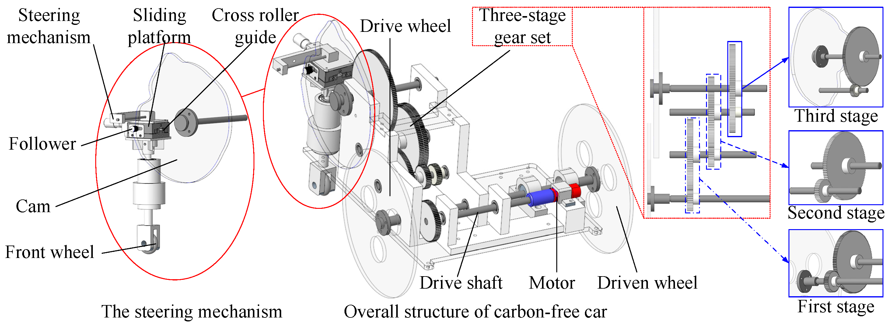
The carbon-free car consists of five components: the prime mover mechanism, the transmission mechanism, the traveling mechanism, the steering mechanism, and a fine adjustment mechanism. The overall structure features a three-wheel configuration, including a front wheel, a driving wheel, and a driven wheel, as depicted in Figure 1.

The prime mover primarily utilizes biomass energy to generate electricity, which in turn drives the motor. The motor is linked to the drive shaft via a coupling, converting the energy into kinetic energy to propel the car forward. During debugging, the prime mover can adjust its driving force according to varying requirements, accommodating different site conditions.

The gear transmission, renowned for its compact design, reliable operation, and stable transmission ratio, utilizes a three-stage gear setup in this car, transferring power from the motor to the steering mechanism with a transmission ratio of $\mathrm{i}$ = 45. The traveling mechanism, which consists of two rear wheels and one front wheel, serves as the final execution component for the car’s motion. The system operates on a single-wheel differential drive principle. One rear wheel is the driven wheel, which is powered directly by the motor through the drive shaft at a constant speed, while the other wheel is idled. In contrast, the driven wheel’s shaft is supported only by two bearings and remains independent of other drive components and motor rotation.

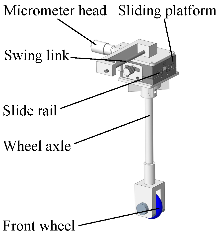
The fine adjustment mechanism comprises a slide rail, a sliding platform movable along the rail, a micrometer head, a front wheel axle, a front wheel, and a swing link. By advancing the micrometer head to drive the sliding platform, the horizontal distance between the front wheel axle and the camshaft axis is adjusted, as shown in Figure 2. This compensates for discrepancies between this distance and the base circle radius value caused by part assembly and machining tolerances. The cylindrical swing link follower and the cam profile form a point-contact sliding pair. The follower’s centerline is co-planar with the camshaft axis and maintains a fixed horizontal position relative to the front axle.

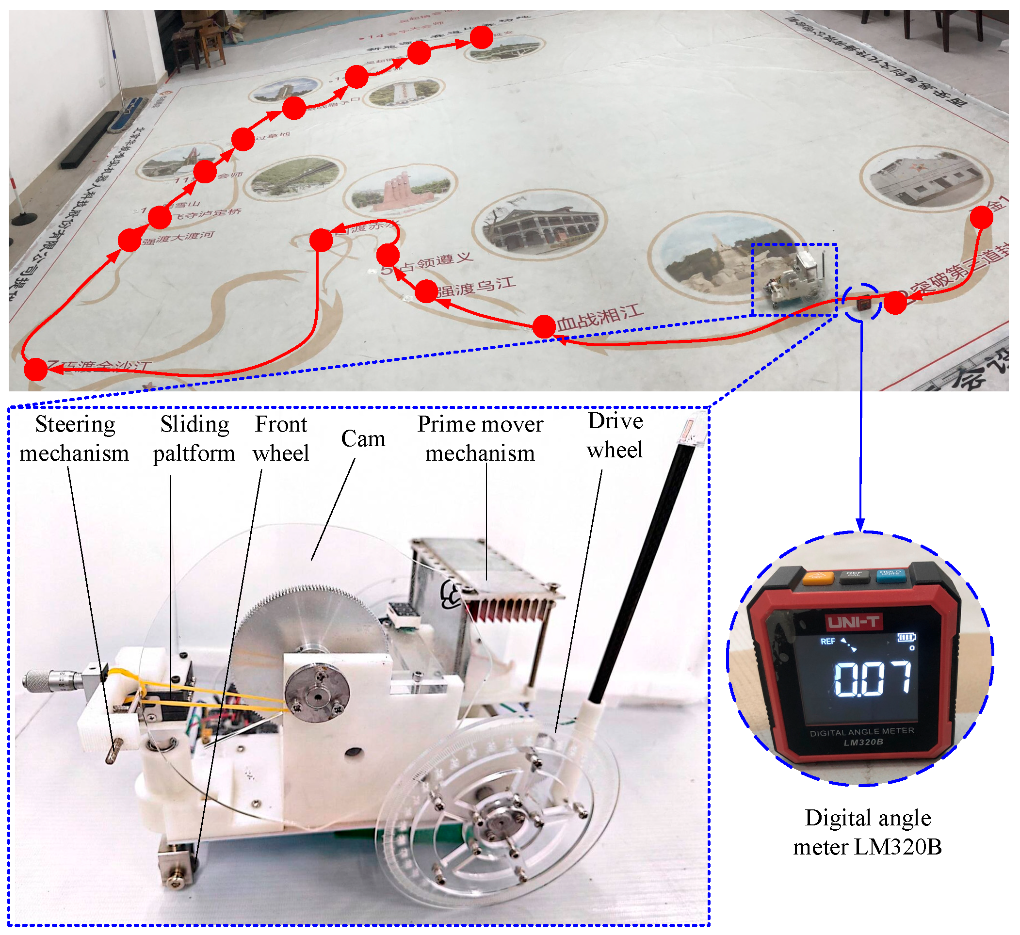
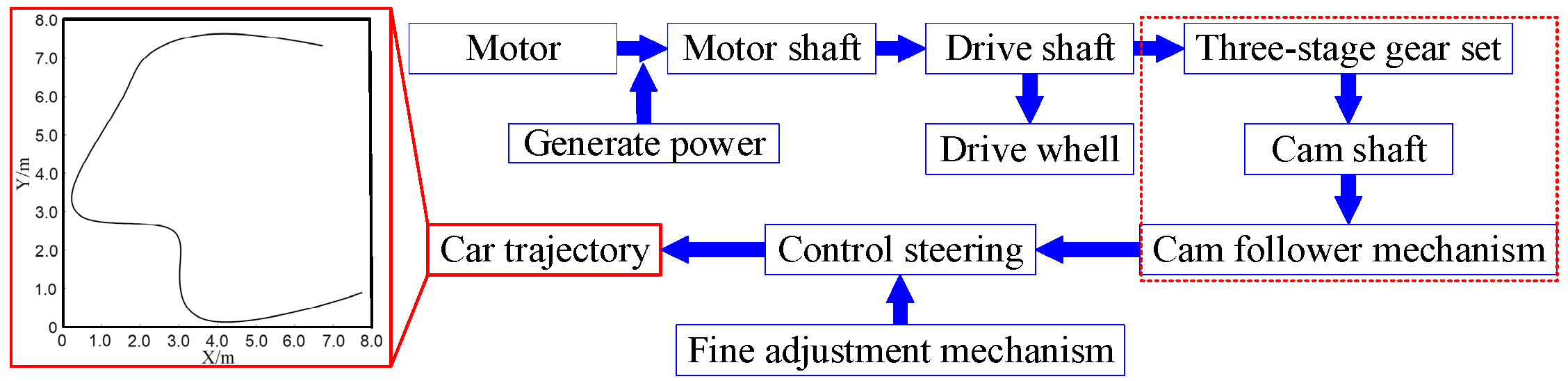
The cam follower mechanism, a key component in the carbon-free vehicle’s steering system, is illustrated in Figure 1. Spring force ensures a constant contact between the cam and the follower. The rotation of the cam converts into the swing of the follower, which in turn guides the front wheel. The complexity of the running track necessitates a specifically designed cam profile to drive the follower in a periodic, expected reciprocating motion, thereby achieving precise steering of the front wheel. Upon the completion of a circular motion by the cam, the car follows the preset motion trajectory. The overall operation process of the carbon-free car is shown in Figure 3. The trajectory that the car in this article needs to follow is shown in Figure 3.

2.2. Analysis of Transmission Error of Gears

The transmission accuracy of gears, as a crucial component of the transmission mechanism, is susceptible to manufacturing and installation errors [30,31] during the construction of carbon-free cars. These errors, categorized as transmission error and return error of gear transmission, significantly impact gear transmission accuracy. This study investigates the influence of the return error of gear transmission on cam steering accuracy.

Return error of gear transmission refers to the delay in rotation angle observed when the output shaft rotates reversely compared to the input shaft due to gear backlash within the gear pair during one-way transmission of the gear mechanism, denoted as $\mathrm{B}$.

2.2.1. Calculation of Maximum Normal Backlash

To determine the maximum normal backlash, it is necessary to calculate the normal backlash resulting from center distance, tooth thickness deviation, base circle eccentricity, and tooth profile error separately [32].

The normal backlash $j_{bn1}$ caused by the increase in center distance is [33]

$$j_{bn1}=2\Delta a\mathit{tan}{\alpha }_n$$

(1)

where $\Delta a$ is the upper deviation of the center distance limit tolerance $+f_{\alpha }$, which can be obtained from the table.

During the gear backlash calculation process, it is crucial to compensate for gear manufacturing error, installation error, thermal expansion deformation, and the minimum gear backlash required for lubrication. The compensation value can be determined based on the negative deviation of the tooth thickness $E_{sni}$. Consequently, the maximum value of the normal backlash caused by a pair of gears $j_{bn2}$ is

$$j_{bn2}=\left|(E_{sni1}+\right.\left.E_{sni2})\right|$$

(2)

To determine the tooth thickness deviation, we must consider the compensation amount $j_n$ to adjust for the decrease in gear backlash resulting from gear machining and installation errors.

$$j_n=\sqrt{\begin{array}{c}{\left(f_{pt1}\mathit{cos}{\alpha }_t\right)}^2+{\left(f_{pt2}\mathit{cos}{\alpha }_t\right)}^2+{\left(F_{\beta 1}\mathit{cos}{\alpha }_n\right)}^2\\ +{\left(F_{\beta 2}\mathit{cos}{\alpha }_n\right)}^2+{\left(f_{\Sigma \delta }\mathit{sin}{\alpha }_n\right)}^2+{\left(f_{\Sigma \beta }\mathit{cos}{\alpha }_n\right)}^2\end{array}}$$

(3)

where $f_{pt1}$ and $f_{pt2}$ represent the base pitch deviations of the gear, retrieved from the table; $F_{\beta 1}$ and $F_{\beta 2}$ denote the total helix deviations of the gear, also sourced from the table; $f_{\Sigma \delta }$ and $f_{\Sigma \beta }$ indicate the parallelism deviations of the gear pair axes; ${\alpha }_t$ and ${\alpha }_n$ denote the end face angle and normal pressure angle of the gear, respectively, with values set at 0° and 20°.

Now we determine the parallelism error of each gear pair’s two gear axes individually, then choose the lesser value. The calculation equation is as follows:

$$f_{\Sigma \beta }=0.5\left({\displaystyle \frac{l}{b}}\right)F_{\beta }$$

(4)

$$f_{\Sigma \delta }=2f_{\Sigma \beta }$$

(5)

where $l$ denotes the bearing span; $b$ represents the tooth width.

The empirical equation for the minimum normal backlash $j_{bnmin}$ is as follows:

$$j_{bnmin}={\displaystyle \frac{2}{3}}(0.06+0.0005a_i+0.03m_n)$$

(6)

where $a_i$ is the minimum working center distance of the gear pair; $m_n$ is the normal module of the gear.

Combining Equations (3) and (6), the positive deviation of tooth thickness $E_{sns}$ can be obtained.

$$E_{sns}=-f_{\alpha }\tan {\alpha }_n-{\displaystyle \frac{j_{bnmin}+j_n}{2\cos {\alpha }_n}}$$

(7)

Before computing the negative deviation of tooth thickness $E_{sni}$, it is essential to establish the tooth thickness tolerance $T_{sn}$.

$$T_{sn}=2\tan {\alpha }_n\sqrt{F_r^2+b_r^2}$$

(8)

where $F_r$ is the radial runout tolerance, obtainable from the table, and $b_r$ is the radial cutting tolerance, obtainable from the table.

Calculate the negative deviation of tooth thickness $E_{sni}$ by combining Equations (7) and (8).

$$E_{sni}=E_{sns}-T_{sn}$$

(9)

By simultaneously solving Equations (2) and (9), we can determine the maximum value of normal backlash $j_{bn2}$. The eccentricity of the base circle and tooth profile errors can be collectively represented by the radial comprehensive error ${\Delta F}_r^{″}$; the resulting gear backlash is $j_{bn3}$.

$$j_{bn3}=2\left({\Delta F}_{r1}^{″}+{\Delta F}_{r2}^{″}\right)\tan {\alpha }_n$$

(10)

where ${\Delta F}_{r1}^{″}$ and ${\Delta F}_{r2}^{″}$ are the comprehensive radial errors of the gear, obtainable from the table.

The calculations above yield the maximum normal backlash $j_{bnmax}$ of a pair of meshing gears.

$$j_{bnmax}=j_{bn1}+j_{bn2}+j_{bn3}$$

(11)

2.2.2. The Calculation Model of Return Error of Gear Transmission

The return error of gear transmission $\mathrm{B}$ produced by each stage of gear pairs is determined by selecting the circumferential backlash $j_{wt}$. The relationship between circumferential backlash $j_{wt}$ and normal backlash $j_{bn}$ is resolved as follows:

$$j_{wt}={\displaystyle \frac{j_{bn}}{\cos {\alpha }_t\cos {\beta }_b}}$$

(12)

where ${\alpha }_t$ represents the end face pressure angle and ${\beta }_b$ denotes the base helix angle, set at 0°.

The correlation between the return error of gear transmission $B$ and the circumferential backlash $j_{wt}$ can be expressed as follows [33]:

$$B={\displaystyle \frac{j_{wt}}{r\times 1000}}\times {\displaystyle \frac{180}{\pi }}$$

(13)

where $r$ signifies the pitch circle radius of the follower gear.

2.3. Modeling of Car Trajectory

The trajectory of the car is the decisive factor in guiding the design of the cam. In MATLAB, a sixth-order B-spline curve [34,35] is derived using interpolation [36] to serve as the trajectory for the carbon-free car. The flexibility of the spline curve is paramount for facilitating the design of complex paths. However, constraints imposed by the car’s structure and the steering characteristics of the cam mechanism necessitate iterative refinement of the trajectory.

The trajectory curve of the car is discretized, with N points evenly distributed along the curve. The X and Y coordinates of these points are recorded as initial data. Combined with Equation (14), the curvature radius $R_1$ at each point is calculated. This trajectory represents the active wheel trajectory of the car, with the left wheel as the active wheel, so $R_1$ is the turning radius of the center point of the left wheel [32].

$$R_1=\left|{\displaystyle \frac{(1+{y^{\prime }}^2{)}^{\frac{3}{2}}}{y^{″}}}\right|$$

(14)

2.4. Car Steering State

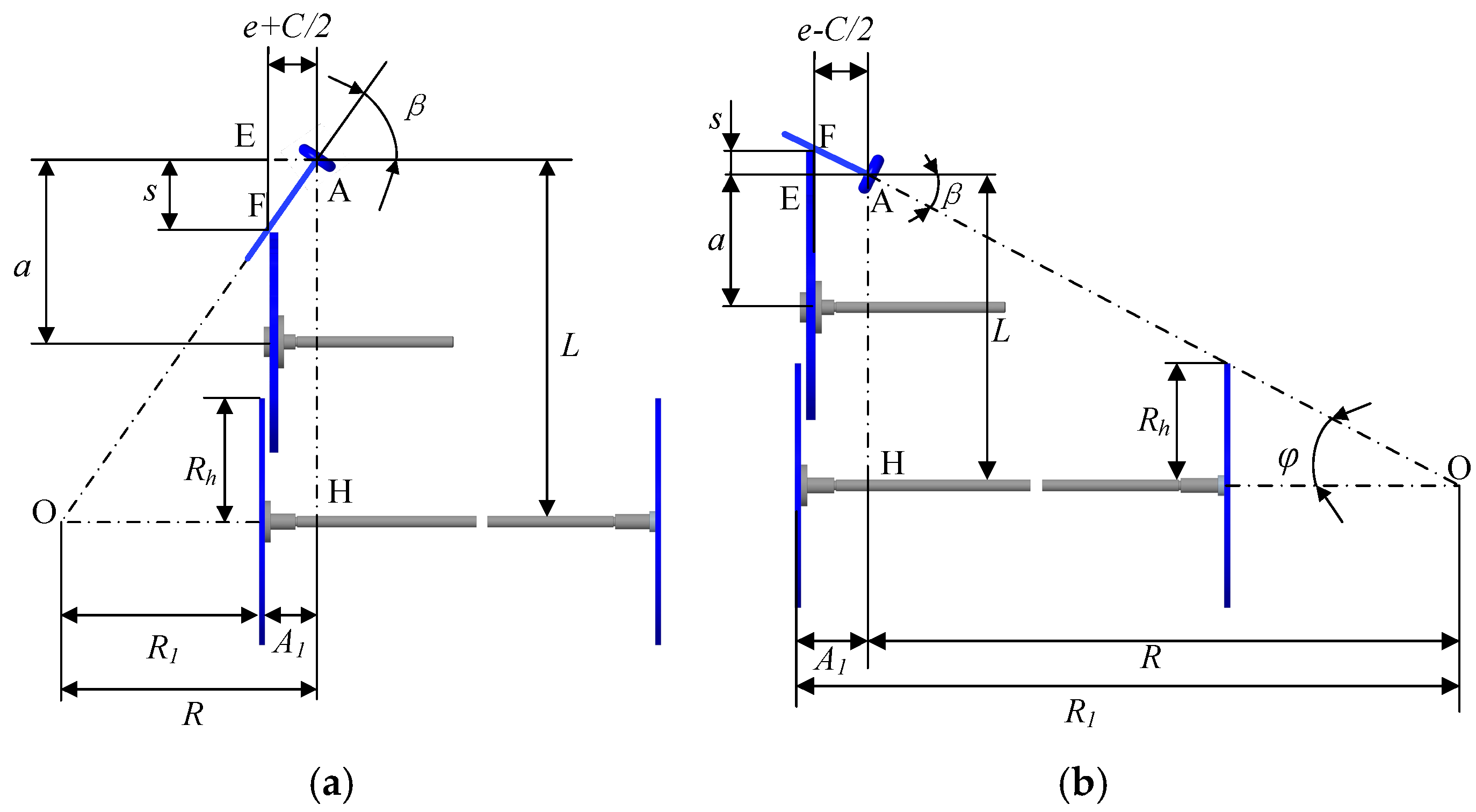
The schematic diagram of the car’s mechanism is presented in Figure 4. The base circle radius of the cam, denoted as a, is defined by the distance from the camshaft to the front wheel center. The incremental displacement of the follower’s contact point relative to this base circle is the lift s. As illustrated in Figure 4b, the lift s takes a positive value during a right turn. Furthermore, the theoretical cam offset distance e represents the axial offset of the cam’s center plane relative to the front wheel center. The wheelbase L is the distance from the front wheel center to the drive shaft, and A₁ denotes the driving wheel offset. The center of the front wheel is taken as the reference point A and the center of the curvature radius of the car at this position is taken as the reference point O; it is assumed that there is a vertical line of the drive shaft through the center of the front wheel, and the foot of the vertical line is taken as the reference point H.

The initial design parameters of the car are shown in

Table 1. Key initial parameters of the car.

Parameter	Initial Value	Parameter	Initial Value
N	3000	a [mm]	70
L [mm]	167	e [mm]	25
A1 [mm]	37	C [mm]	3
A2 [mm]	201	rt [mm]	2.5

. Among these, $A_2$ represents the offset distance of the right wheel, and $r_t$ stands for the follower’s radius.

2.5. The Theoretical Model of Cam Profile

Taking into account the thickness of cam C, the actual cam offset e_r represents the distance from the center point A of the front wheel to the cam plane, wherein the actual contact point F of the follower and the cam is situated [37].

$$e_{\mathrm{r}}=\left\{\begin{array}{c}e+{\displaystyle \frac{C}{2}} \left(\mathrm{s}<0\right)\\ e-{\displaystyle \frac{C}{2}} \left(\mathrm{s}\ge 0\right)\end{array}\right.$$

(15)

In the triangular AEF, the deflection angle $\beta$ of the car follower in relation to the push stroke s is represented as follows:

$$tan\beta =\left\{\begin{array}{c}{\displaystyle \frac{s}{e+\frac{C}{2}}} (s<0)\\ 0 (s=0)\\ {\displaystyle \frac{s}{e-\frac{C}{2}}} (s>0)\end{array}\right.$$

(16)

In the triangular AHO,

$$tan\beta ={\displaystyle \frac{L}{R}}$$

(17)

From Figure 4, we derive the connection between the steering radius $R$ at reference point H and $R_1$ as follows:

$$R=\left\{\begin{array}{c}{R}_1+A_1\left(s\le 0\right)\\ R_1-A_1\left(s>0\right)\end{array}\right.$$

(18)

The equations of the push stroke can be acquired from Equations (16)–(18) simultaneously, as stated below.

$$s=\left\{\begin{array}{c}{\displaystyle \frac{L\times \left(e+\frac{C}{2}\right)}{R_1+A_1}} \left(s\le 0\right)\\ {\displaystyle \frac{L\times \left(e-\frac{C}{2}\right)}{R_1-A_1}} \left(s>0\right)\end{array}\right.$$

(19)

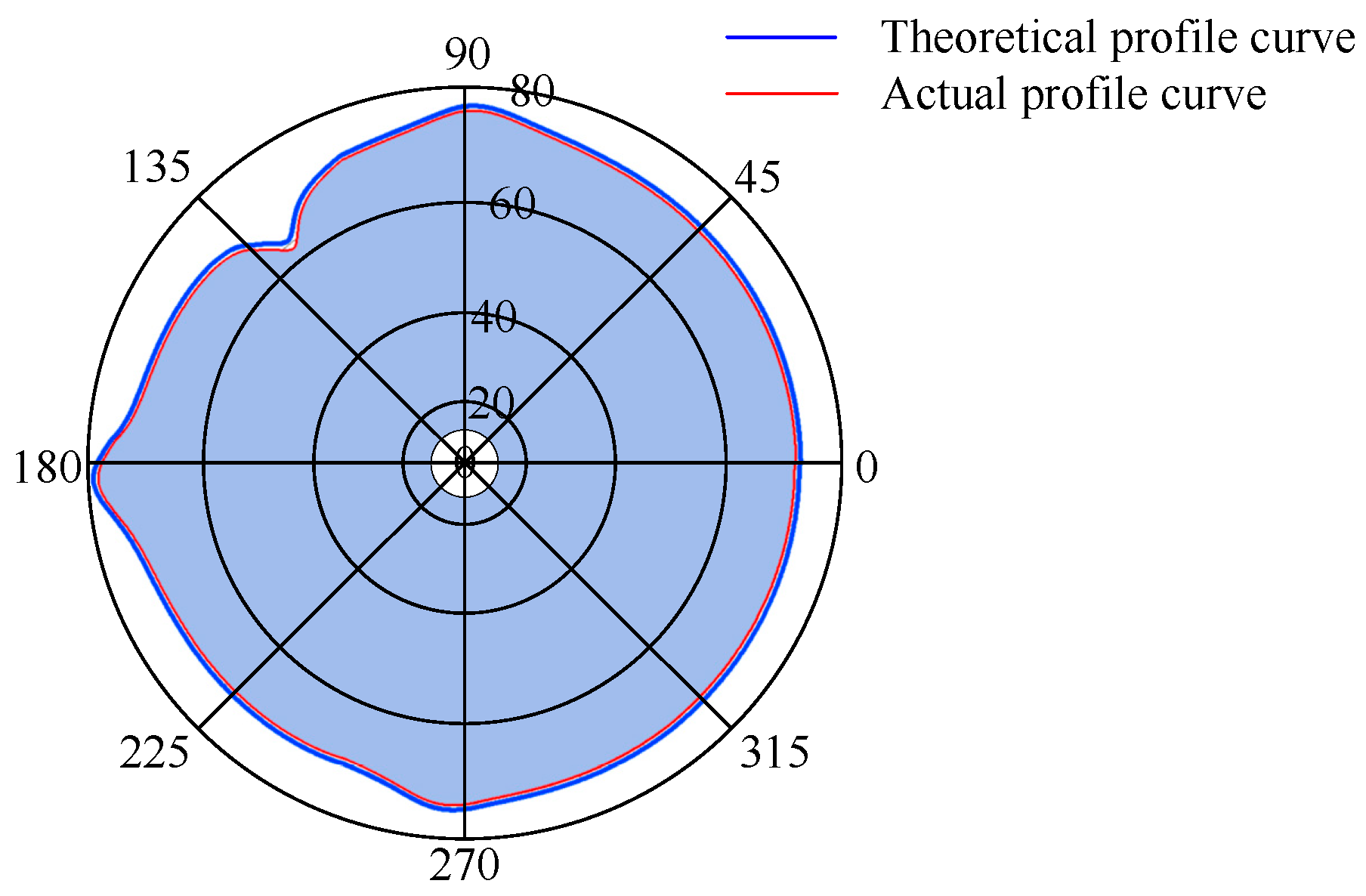
By substituting the initial parameters of the carriage, we ascertain the cam stroke s, leading to the depiction of the resulting cam profile curve in Figure 5.

2.6. The Theoretical Model of Car Trajectory

Applying a forward calculation method for calculation, the designed cam profile curve is utilized to forwardly deduce the spliced running trajectory. Differential operations are conducted on the car’s motion to derive changes in the front wheel steering angle $d\beta$, cam angle $d\theta$, and displacement variation in the driving wheel of the car $dx$ within each differential motion interval. The motions within each interval are overlaid to generate the car’s motion trajectory curve.

The relationship between the cam angle variation $d\theta$ and displacement variation in the driving wheel of the car $dx$ is as follows [37]:

$${\displaystyle \frac{dx}{2\pi R_{h}i}}={\displaystyle \frac{d\theta }{360}}$$

(20)

The angle $\beta$ turned by the carriage relative to its initial state can be determined by considering that the initial position of the active wheel center of the carriage is ($X_0$, $Y_0$), the initial angle formed by the direction of the car body and the X-axis is ${\beta }_0$, and the linear velocity of the active wheel of the carriage is $v_1$; then, the angle $\beta$ turned by the carriage relative to the initial state is [31]

$$\beta =-\int {\displaystyle \frac{s{v}_1}{L\left(e-\frac{\left|s\right|C}{2s}\right)+s{A}_1}}dx$$

(21)

The angle ${\beta }_1$ between the direction of the car body and the X-axis is

$${\beta }_1={\beta }_0+\beta$$

(22)

The formula describing the coordinates of the center point of the driving wheel ($x_1$, $y_1$) in motion is

$$\left(\begin{array}{c}{x}_1\\ y_1\end{array}\right)=\left(\begin{array}{c}{X}_0-\int v_1\sin \beta dx\\ Y_0-\int v_1\cos \beta dx\end{array}\right)$$

(23)

By referring to Equation (25) along with Figure 5, we can derive the expressions for the motion coordinates of the center point of the front wheel ($x_0$, $y_0$) and the center point of the driven wheel ($x_2$, $y_2$) [31]:

$$\left(\begin{array}{c}{x}_0\\ y_0\\ x_2\\ y_2\end{array}\right)=\left(\begin{array}{c}{x}_1-L\sin \beta +A_1\cos \beta \\ y_1-L\cos \beta +A_1\sin \beta \\ x_1+(A_1+A_2)\cos \beta \\ y_1+(A_1+A_2)\sin \beta \end{array}\right)$$

(24)

3. The Numerical Calculation Results of the Return Error of Gear Transmissions of Each Transmission Mechanism of the Car

Based on theoretical formulae, the backlash and return error in the multi-stage gear transmission were computed for the initial design. The car’s kinematic trajectory was simulated via MATLAB and contrasted with the original trajectory. This work also involved a systematic investigation into the influence of gear transmission errors on cam steering precision. The investigation yielded results for the original deflection error (in both travel and deflection angle), as well as the trajectories under three specific error scenarios: jumping error only, return error only, and the combined influence of both.

3.1. The Calculation Result of the Return Error of the Gear Transmission of the Three-Stage Gear Set Transmission

The car utilizes a three-stage spur gear transmission as its transmission mechanism, with a precision grade of 7. The relevant basic parameters are outlined in

Table 2. Basic parameters of transmission gears.

Transmission Grade $\mathit{j}$	First Stage	Second Stage	Third Stage
Transmission ratio $i_n$	5	3	3
Center distance $a_i$ [mm]	45	40	40
Modulus $m_n$ [mm]	0.5	0.5	0.5
Bearing span $l$ [mm]	80	80	80
Tooth width $b$ [mm]	5	5	5
Number of gear teeth	150/30	120/40	120/40
Normal pressure angle ${\alpha }_{\mathrm{n}}$ [°]	20
End face angle ${\alpha }_{\mathrm{t}}$ [°]	0
Modulus mn [mm]	0.5

. By substituting the basic parameters outlined in Table 2 into Equations (1)–(13), the corresponding parameters for each gear pair can be derived as shown in

Table 3. Related parameters of gear pairs at all levels.

$\mathit{j}$	${\mathit{j}}_{\mathit{b}\mathit{n}1}$ [µm]	${\mathit{j}}_{\mathit{b}\mathit{n}2}$ [µm]	${\mathit{j}}_{\mathit{b}\mathit{n}3}$ [µm]	${\mathbf{j}}_{\mathbf{b}\mathbf{n}\mathbf{m}\mathbf{a}\mathbf{x}}$ [µm]	${\mathit{B}}_{\mathit{n}}$ [°]
First stage	14.195	302.324	39.309	355.828	0.544
Second stage	14.195	300.550	39.309	354.054	0.676
Third stage	14.195	300.550	39.309	354.054	0.676

.

The car’s transmission mechanism comprises a three-stage gear transmission. It is imperative to compute the cumulative impact of multiple gear pairs within the transmission chain, denoted as the comprehensive return error of gear transmission $B_{\mathrm{\Sigma }}$. The relationship between the comprehensive return error of gear transmission $B_{\mathrm{\Sigma }}$ and the return error of the gear transmission of each stage gear pair $B_n$ is expressed as follows [33]:

$$B_{\Sigma }=B_n+{\displaystyle \frac{B_{n-1}}{i_n}}+{\displaystyle \frac{B_{n-2}}{i_n{i}_{n-1}}}+\cdots +{\displaystyle \frac{B_1}{i_n{i}_{n-1}\cdots i_2}}=\sum _{j=1}^n{\displaystyle \frac{B_j}{i_{jn}}}$$

(25)

$$i_{jn}={\prod }_{k=j+1}^n{i}_k$$

(26)

where $i_{jn}$ is the ratio from the driven shaft of the $j$-stage gear pair to the output shaft of the transmission chain, namely the transmission ratio to the camshaft.

By inputting the maximum return error of gear transmission of each gear pair into Equations (25) and (26), we derive the comprehensive return error of gear transmission ${\mathrm{B}}_{\Sigma }$ = 0.962°.

3.2. Numerical Analysis of Car Trajectory

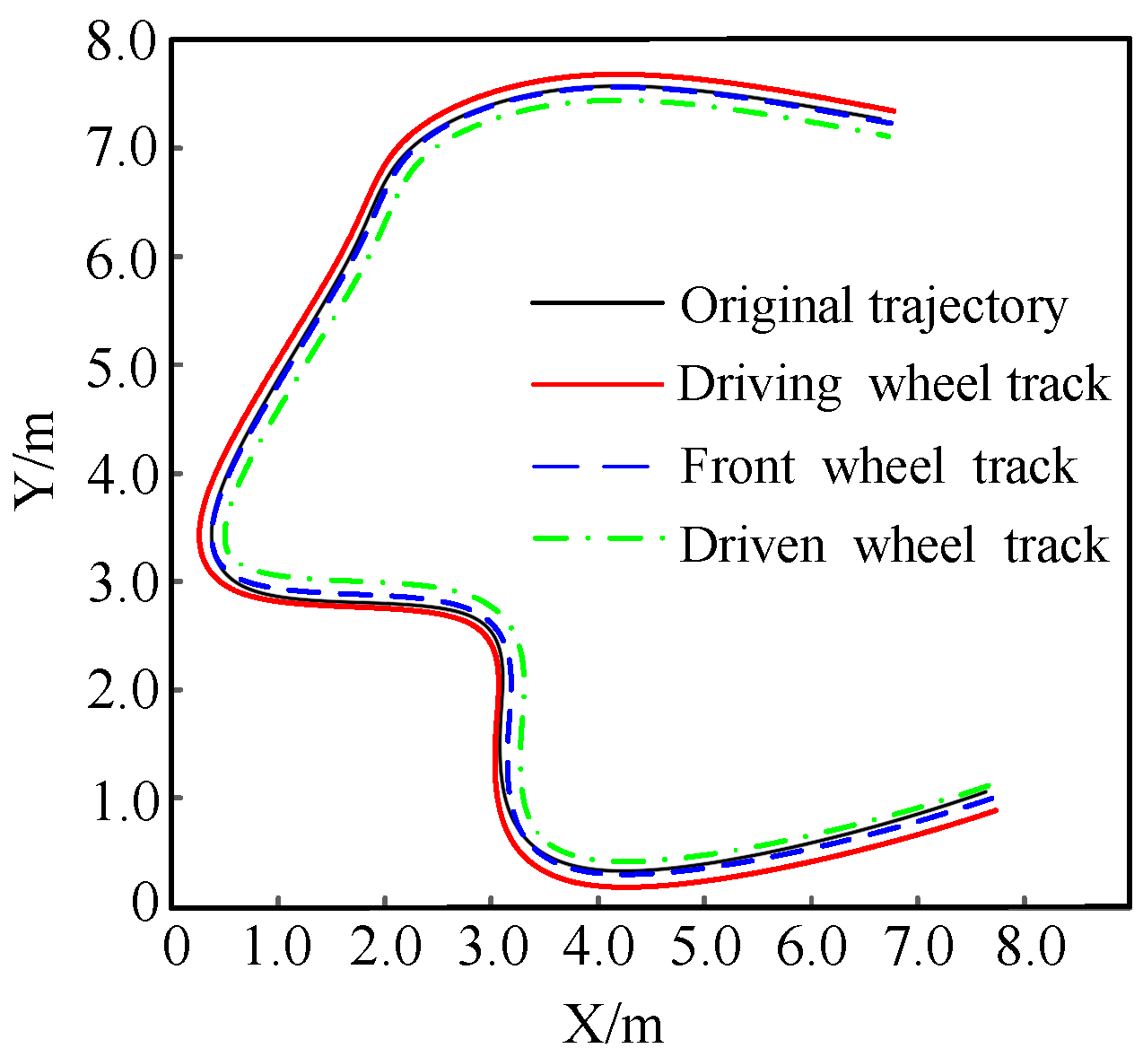
Figure 6 shows the comparison between the calculated trajectory of the car and the original trajectory. The calculated trajectories of the three wheels are three curves with equal spacing. Among them, the calculated trajectory of the front wheel coincides with the original trajectory when Y > 3 m, and there is a slight deviation when Y < 3 m. The reason is that the return error of gear transmission of the gear transmission affects the accuracy of the cam transmission, thus affecting the steering accuracy. The optimization of the cam profile can be used to improve the accuracy of the cam transmission, thereby improving the steering accuracy.

3.3. The Influence of the Return Error of Gear Transmission of the Gear Set Transmission on Cam Steering Accuracy

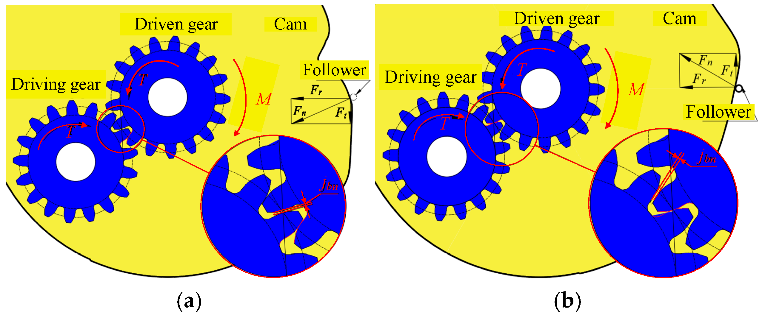
During transmission, the driven gear undergoes transmission torque $T$ in the direction depicted in Figure 7a. This torque is utilized to oppose the load torque $\mathrm{M}$ applied by the follower, while maintaining the gear pair in a standard meshing state.

As the follower traverses the jump point, the negative torque exerted by the follower on the cam undergoes reversal, aligning with the transmission torque received by the driven gear, which is coaxial with the cam. Owing to the presence of gear backlash $j_{bn}$, the driven gear experiences a slight angular displacement under the influence of the negative torque, equivalent to the comprehensive return error of the gear transmission $B_{\Sigma }$ calculated previously. This scenario, referred to as the jump return error of gear transmission, results in the disengagement of originally meshed teeth at the working surfaces, while the non-working surfaces come into contact with each other, as illustrated in the enlarged image in Figure 7b.

As the follower crosses the reverse point, the load torque applied by the follower to the cam opposes the driving torque exerted by the driven gear. This transition alters the meshing state of the gear pair from the configuration depicted in Figure 7b to the state illustrated in the partially enlarged view of Figure 7a, causing the driven gear to rotate slightly under the influence of the load torque. Let the return error of the gear transmission in this scenario be termed the reverse return error of the gear transmission.

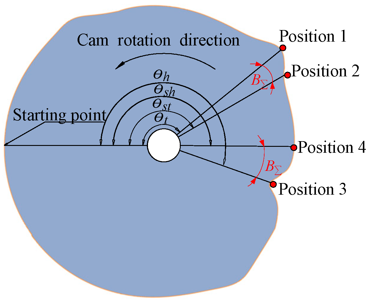
As the driven gear is coaxial with the cam, the cam also undergoes a slight angular displacement, causing the follower to transition from position 1 to position 2. Consequently, the cam profile corresponding to this slight angle becomes invalid, as depicted in Figure 8. Given that the driven gear is coaxial with the cam, the cam also rotates by the same small angle. Consequently, the follower returns from position 3 to position 4, enabling the repeated action of the cam profile corresponding to the tiny angle, as depicted in Figure 8.

$${\theta }_{st}={\theta }_t+B_{\sum }$$

(27)

where ${\theta }_{st}$ represents the cam angle after the jump and ${\theta }_t$ represents the cam angle before the jump [26].

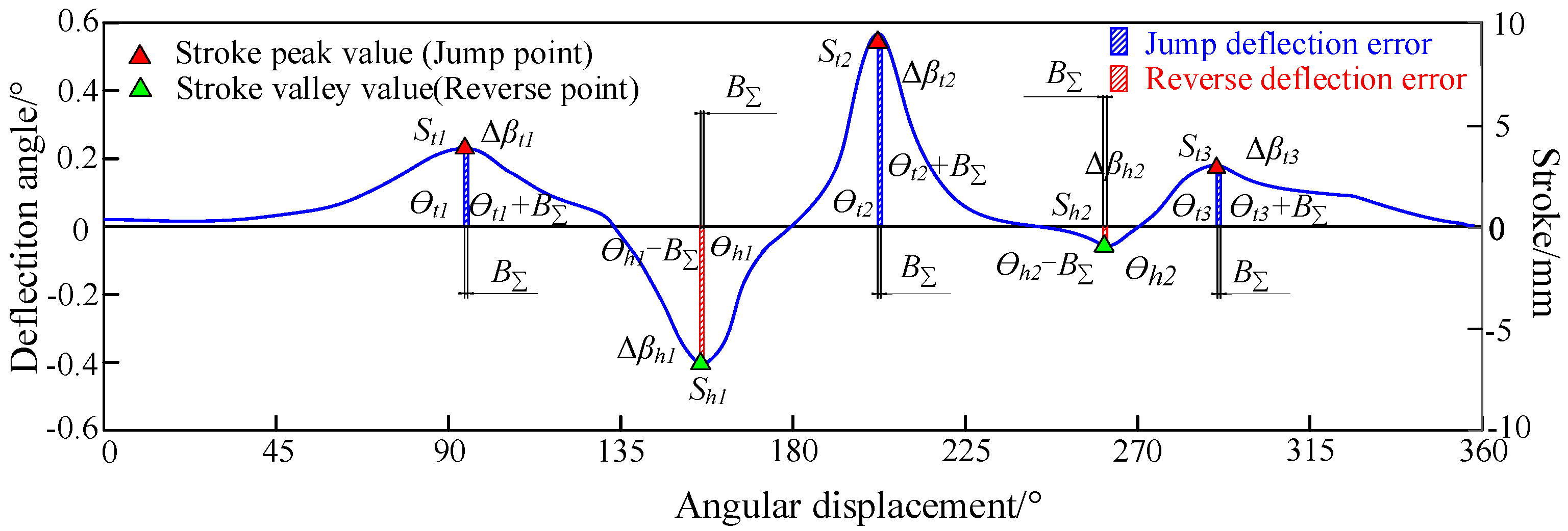
During the steering process of the cam, as the follower moves from the push stroke area to the return stroke area, the contact point between the follower and the cam becomes a jump point. Similarly, when the follower transitions from the return stroke area to the push stroke area, it becomes the reverse point, as depicted in Figure 9.

If a segment of the cam profile malfunctions, the follower’s swing angle in that section will not be imparted to the car’s actual moving path. When considering Equations (20) and (21), it becomes apparent that the original cumulative deflection angle of the car undergoes a change, represented as the jump deflection error ${∆\beta }_t$, as depicted in Figure 9:

$${∆\beta }_{\mathrm{t}}={\int }_{{\theta }_t}^{{\theta }_{st}}{\displaystyle \frac{\pi R_{h}is{v}_1}{180\left[L\left(e-\frac{\left|s\right|C}{2s}\right)+s{A}_1\right]}}d\theta$$

(28)

where ${\theta }_{sh}$ represents the cam angle after the reverse and ${\theta }_h$ represents the theoretical cam angle before the reverse.

The repetitive action of the cam profile results in the corresponding deflection angle of the follower in this section of the profile curve being reflected twice in the trajectory of the car. Consequently, the actual original cumulative deflection angle of the car undergoes alteration, denoted as the reverse deflection error ${∆\beta }_h$, as depicted in Figure 9.

$${\theta }_{sh}={\theta }_h-B_{\sum }$$

(29)

$${∆\beta }_h=-{\int }_{{\theta }_{sh}}^{{\theta }_h}{\displaystyle \frac{\pi R_{h}is{v}_1}{180\left[L\left(e-\frac{\left|s\right|C}{2s}\right)+s{A}_1\right]}}d\theta$$

(30)

When the car crosses a jump point (or reverse point), its trajectory shifts to the left compared to the theoretical path. Subsequently, passing through the same point amplifies this deviation. With each additional encounter of jump points (or reverse points), the cumulative error effect grows, leading to increasingly significant deflection errors in the car’s path.

Table 4. Original deflection error of cam follower.

Return Error of Gear Transmission	Code	$\mathit{s}$ [mm]	Code	$∆\mathit{\beta }$ [°]	${∆\mathit{\beta }}_{\mathit{z}}$ [°]
Jump zone	$s_{\mathrm{t}1}$	5.848	${∆\beta }_{t1}$	2.721	17.154
	$s_{\mathrm{t}2}$	9.425	${∆\beta }_{t2}$	6.695
	$s_{\mathrm{t}3}$	3.683	${∆\beta }_{t3}$	2.151
Reverse zone	$s_{\mathrm{h}1}$	−9.065	${∆\beta }_{h1}$	4.879
	$s_{\mathrm{h}2}$	−0.917	${∆\beta }_{h2}$	0.709

illustrates the respective jump deflection error ${∆\beta }_t$ and reverse deflection error ${∆\beta }_{\mathrm{h}}$, and ${∆\beta }_{\mathrm{z}}$ represents the original cumulative deflection error.

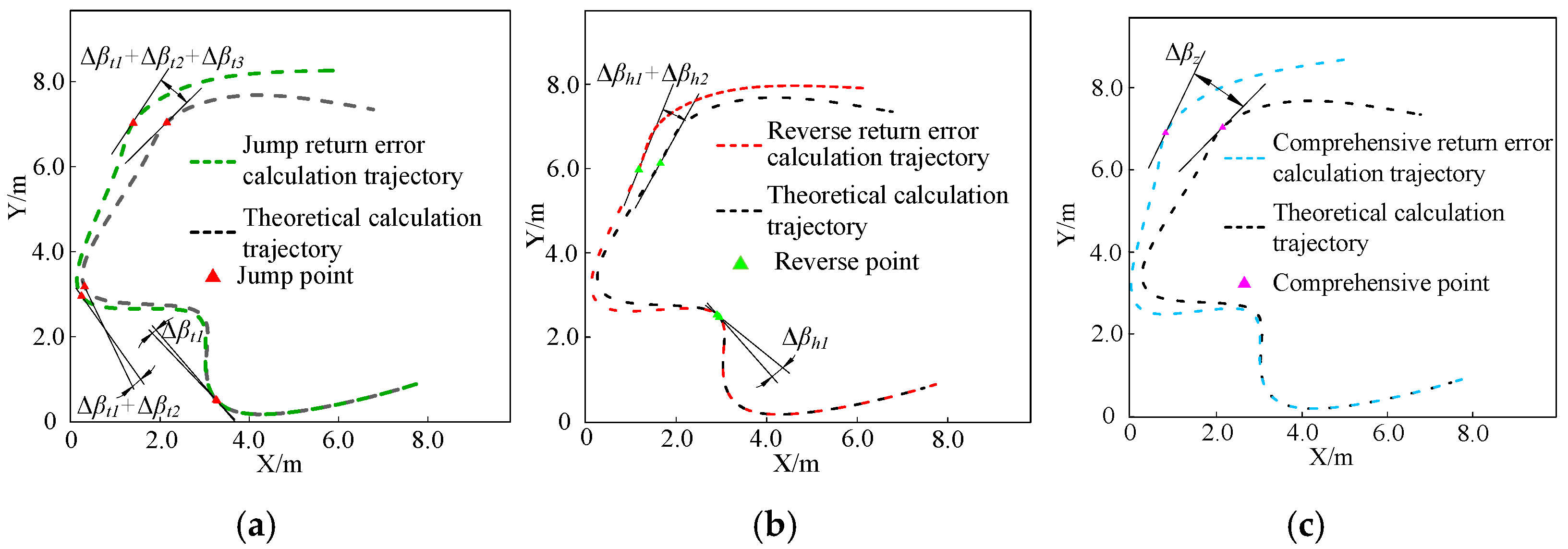
Through mathematical modeling, the effect of gear return error of gear transmission on the car trajectory was analyzed. However, qualitative analysis alone proved insufficient to clearly reveal this influence. Therefore, a MATLAB calculation was employed to generate the trajectory under the return error of gear transmission, which was then compared with the theoretical path. By plotting tangents at jump or reverse points on both trajectories, the angle between them was used to quantify the cumulative deviation error at these positions. This enabled a quantitative assessment of trajectory deviation.

The car’s pre-optimization trajectory is illustrated in Figure 10. Specifically, Figure 10a only considered the jump return error of gear transmission for trajectory calculation analysis; it was observed that the jump return error of gear transmission leads to the failure of the follower deflection angle $\phi$ corresponding to the cam contour segment, resulting in a reduced original cumulative deflection angle to the right, denoted as ${∆\beta }_t$. Subsequent calculation trajectories deviate to the left, with the error increasing as the number of jumps increases. Figure 10b only incorporated the reverse return error of the gear transmission for trajectory calculation analysis. It was found that the reverse return error of the gear transmission causes repetitive action of the follower deflection angle $\phi$ corresponding to the cam contour segment, leading to an increased original cumulative deflection angle towards the left, denoted as ${∆\beta }_h$. Subsequent calculation trajectories of the car deviate to the left.

Trajectory calculation analysis incorporating both the jump return error of the gear transmission and the reverse return error of the gear transmission was conducted. Throughout a motion cycle, the cam experiences three jump points and two reverse points, generating corresponding jump return and reverse return error of gear transmissions. The error accumulation effect is depicted in Figure 10c.

4. Optimization and Numerical Calculation of Cam Trajectory with Consideration of Return Error of Gear Transmission

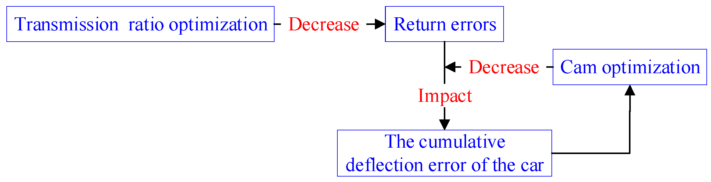
To reduce the gear transmission return error and thereby optimize the steering accuracy of the cam, two methods were employed: adjusting the gear ratio and optimizing the cam profile. Furthermore, the synergistic effect of combining both methods was analyzed for a comprehensive optimization.

4.1. Optimization Measures

The optimization measures for the car trajectory include adjusting the gear ratio and optimizing the cam profile. Based on the above two optimization perspectives, the trajectory deviation of the car was analyzed. Among them, optimizing the cam profile was characterized by adjusting the peak and valley values of the push stroke at the jump and reverse points. The optimization process is shown in Figure 11.

4.1.1. Adjust the Transmission Ratio of the Gear Transmission

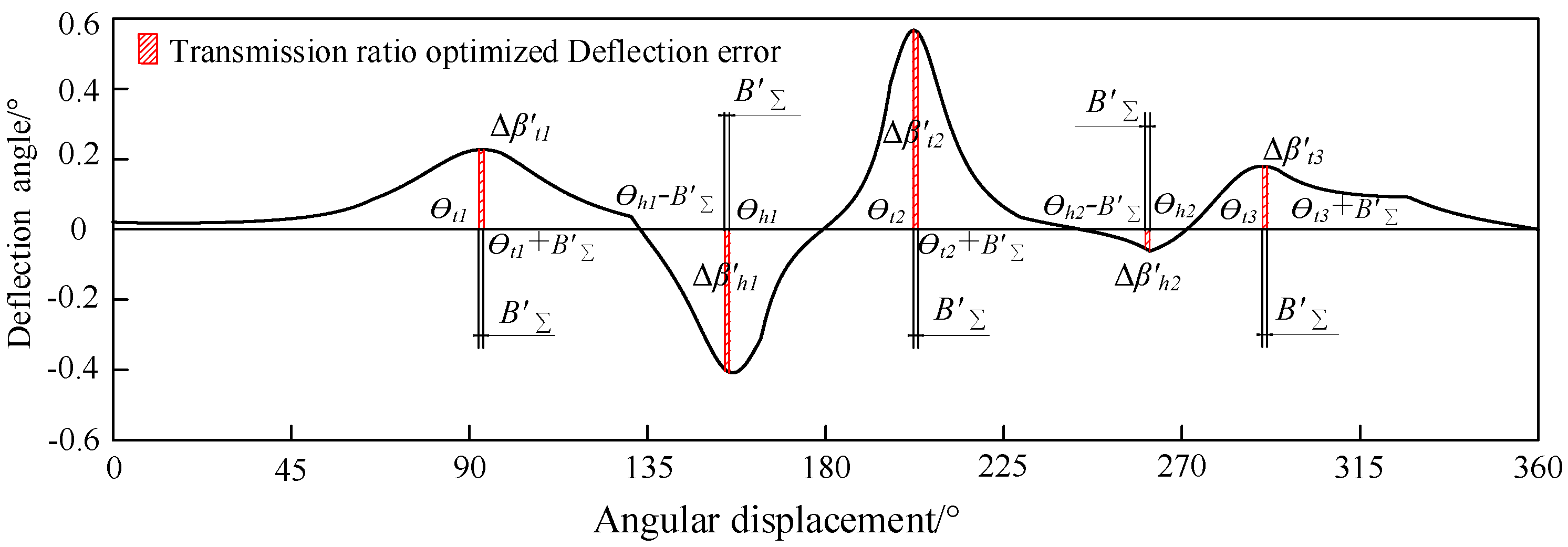
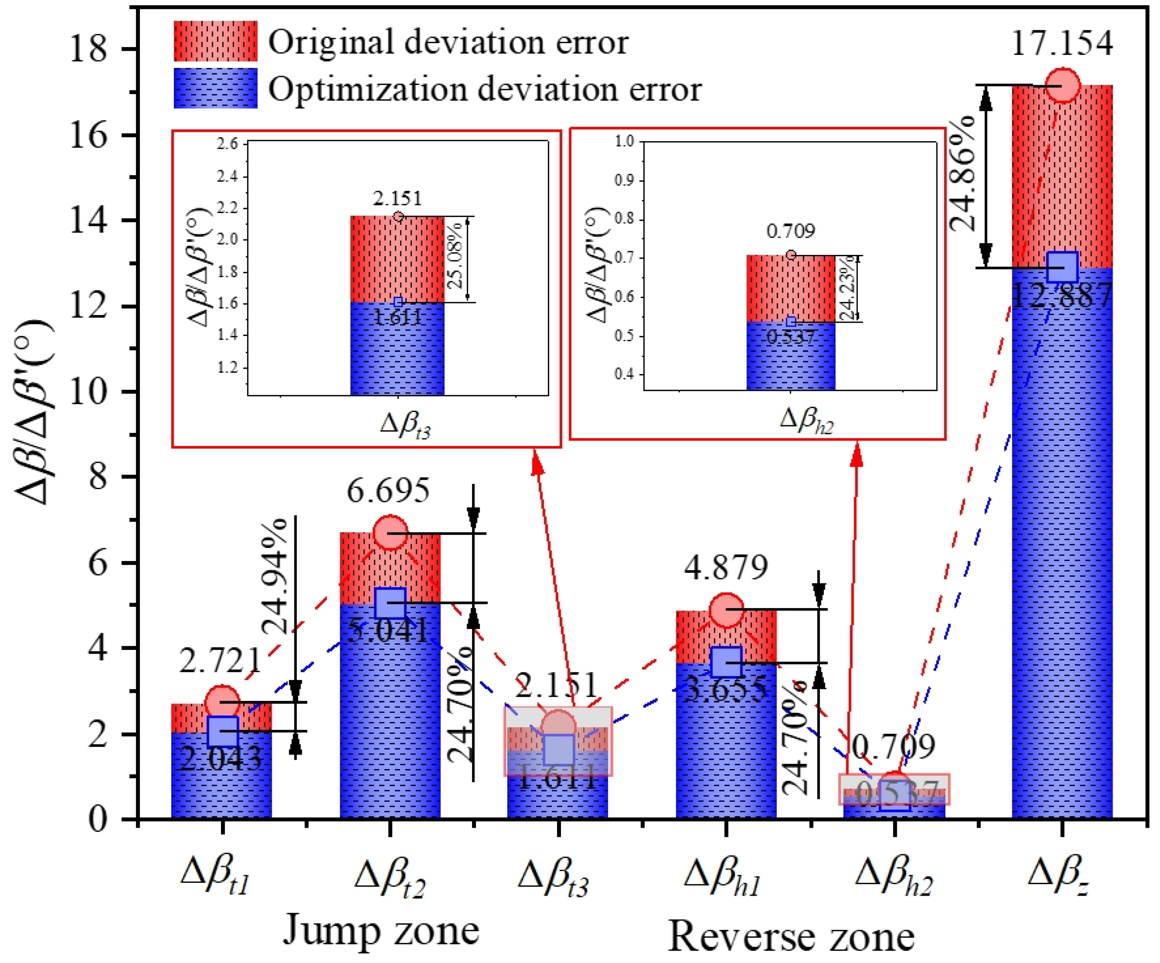
From Equation (20), the analysis reveals that the gear transmission backlash (return error) generated at each stage of the gear train is amplified by the transmission ratio of subsequent stages as it propagates toward the output shaft. Consequently, the backlash originating from the final gear pair has the most dominant effect on the resulting angular deviation of the output shaft. Therefore, if the structure allows, the transmission ratio of the last stage in the transmission chain should be increased to diminish the impact of the front stage’s return error of gear transmission on the output shaft angle. Without altering the total transmission ratio, the stage with the highest transmission ratio is positioned at the end; specifically, the transmission ratio at the third stage is 5. By substituting the modified transmission ratios of each stage into Equations (25) and (26), the optimized overall return error of the gear transmission $B_{\Sigma }^{\prime }$ = 0.724° is obtained, which is a reduction from the original overall return error of the gear transmission $B_{\Sigma }$ = 0.962°, as shown in Figure 12. The optimization of the cumulative deflection error ${∆\beta }_z^{\prime }$ after adjusting the transmission ratio is 24.74% compared to the original cumulative deflection error ${∆\beta }_z$, as demonstrated in Figure 13. Adjusting the gear ratio effectively reduced the deflection error, but at the expense of requiring modifications to the overall structure, which complicated the gear set design process and made assembly more difficult.

4.1.2. Optimizing the Cam Profile

Given that mitigating the front stage’s return error of gear transmission solely through transmission ratio adjustment is constrained by structural and ratio suitability factors, a multi-faceted approach is required. Beyond increasing the rear stage transmission ratio, this solution also involves optimizing the peak and valley values of the push stroke at the jump and reverse points. This serves to minimize the resulting deflection error and thereby enhances the cam’s steering precision.

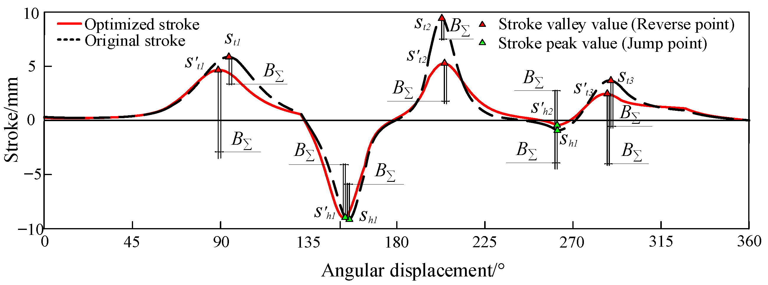
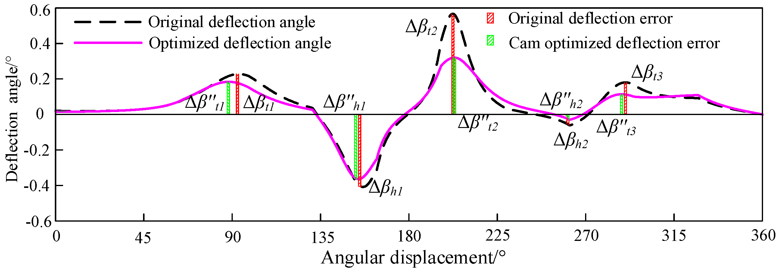
From Equation (21), it is observed that the absolute value of the stroke s is directly proportional to the deflection error induced by the return error of gear transmission. Consequently, with the return error of gear transmission remaining constant, the cam profile is optimized to smooth the fluctuations of the peak and valley values of the stroke at the jump and reverse points, as illustrated in Figure 14. This adjustment aims to diminish the impact of the return error of gear transmission on the deflection angle during the car’s operation, as depicted in Figure 15.

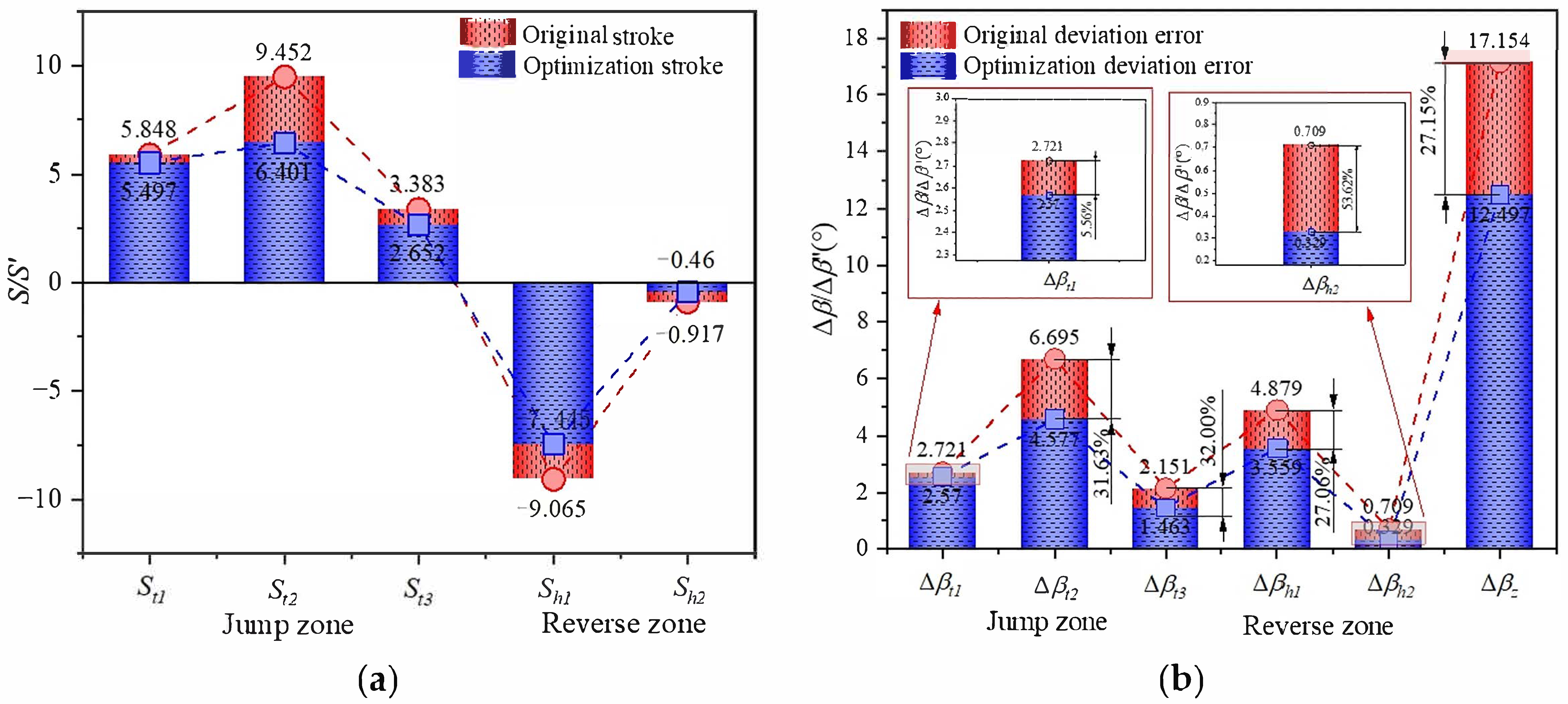
As shown in Figure 16, the optimization of the cam profile resulted in a 27.15% reduction in the deflection angle error compared to the original design, where both stroke and deflection angle are illustrated before and after optimization. Specifically, Figure 16a corresponds to the travel deviation before and after optimization shown in Figure 14, while Figure 16b corresponds to the deflection angle deviation before and after optimization shown in Figure 15. While the optimization of the cam profile significantly enhanced steering accuracy, this came with the drawback of a more intricate actual machining path and more demanding requirements for machining precision.

4.1.3. Comprehensive Optimization

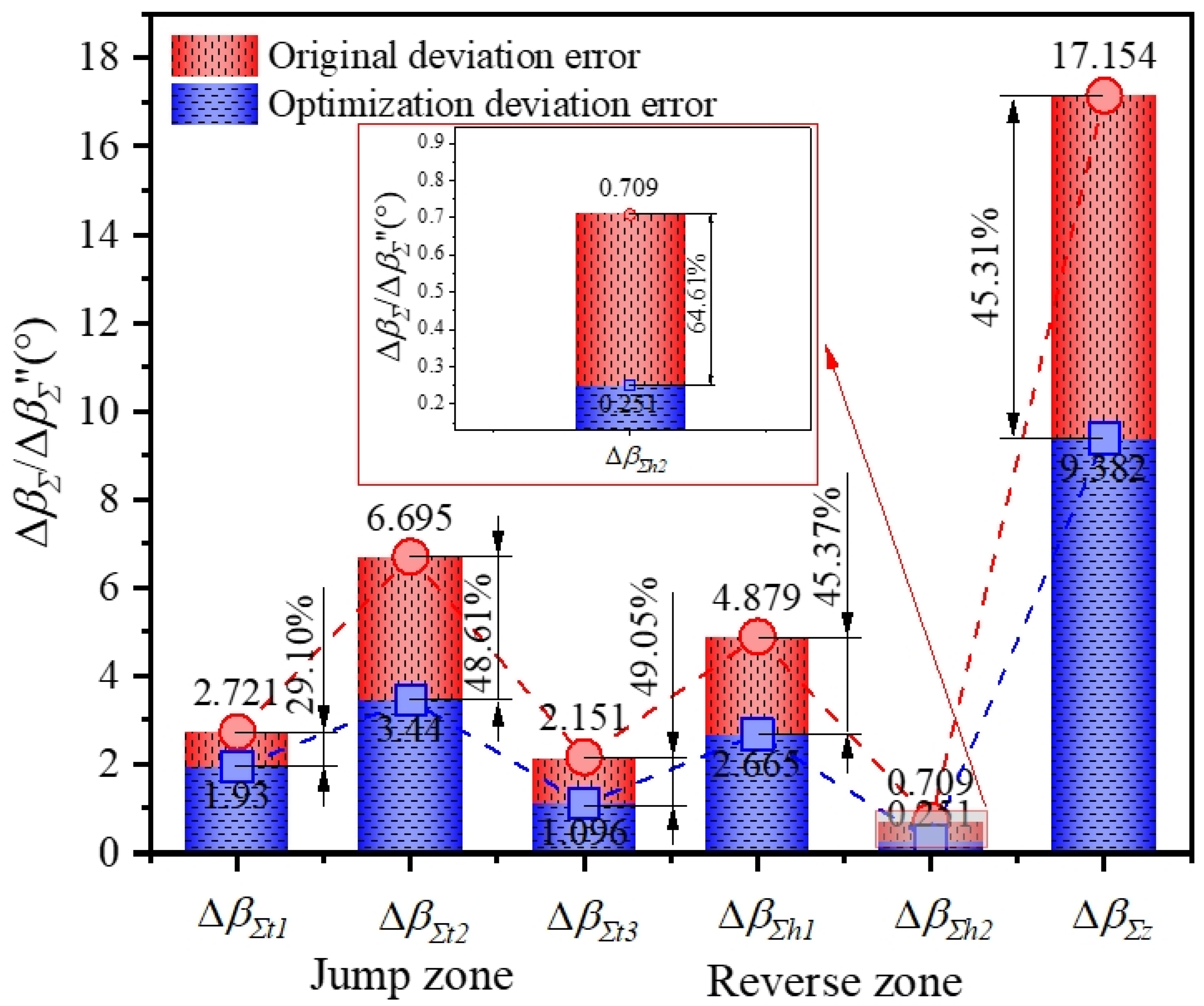
Figure 17 shows the comparison of the optimization effect between the cumulative deflection error ${∆\beta }_z^{″}$ of the comprehensive optimized cam and the original cumulative deflection error ${∆\beta }_z$. Combining the two optimization methods mentioned above, on the basis of transmission ratio optimization, the cam profile curve can be further optimized. In contrast to the cumulative deflection error of the comprehensive optimization result ${∆\beta }_{\Sigma z}$, with the original cumulative deflection error ${∆\beta }_z$, the comprehensive optimization effect reaches 45.31%. The optimization results are shown in Figure 17.

4.2. The Optimized Trajectory of the Car

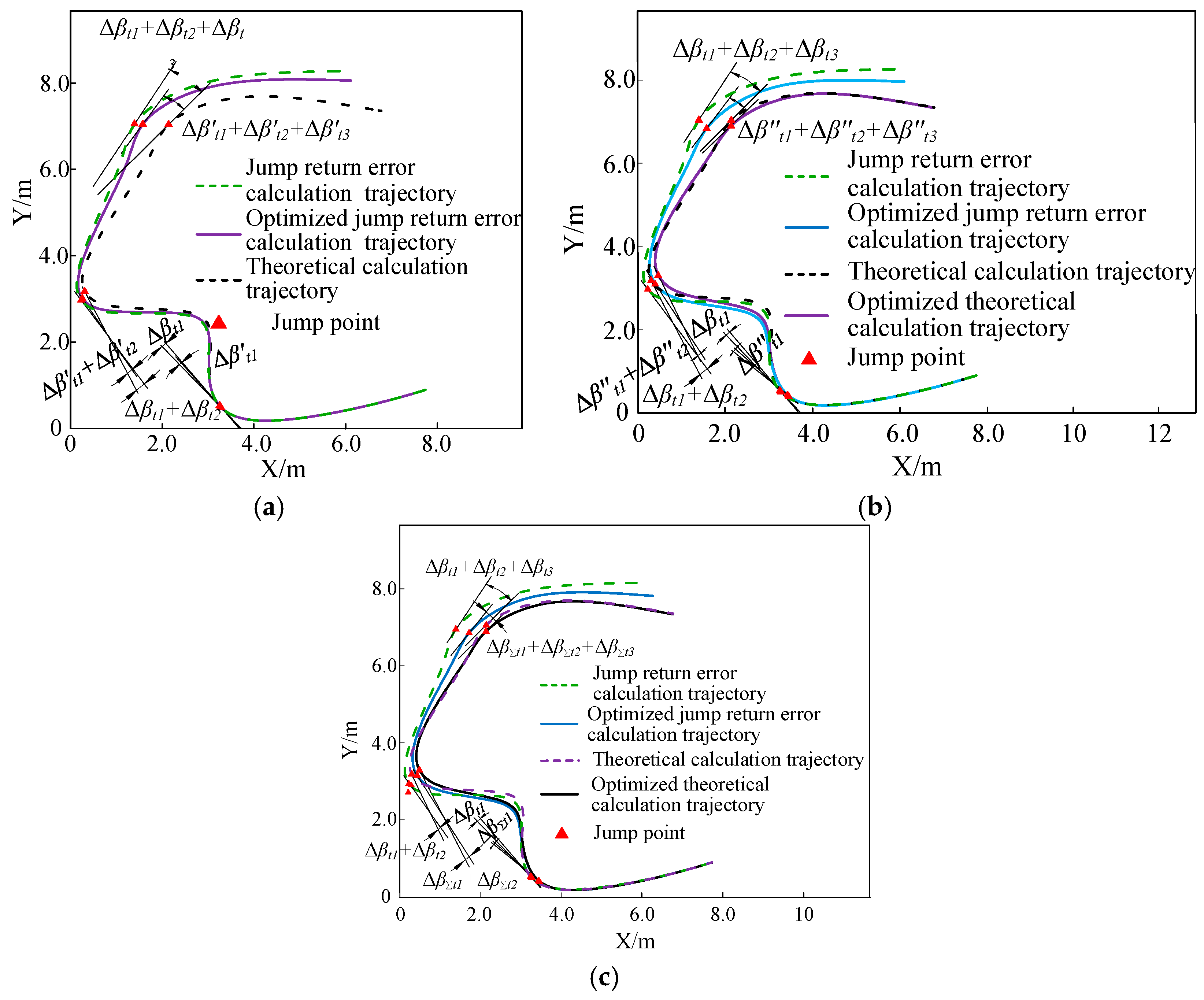
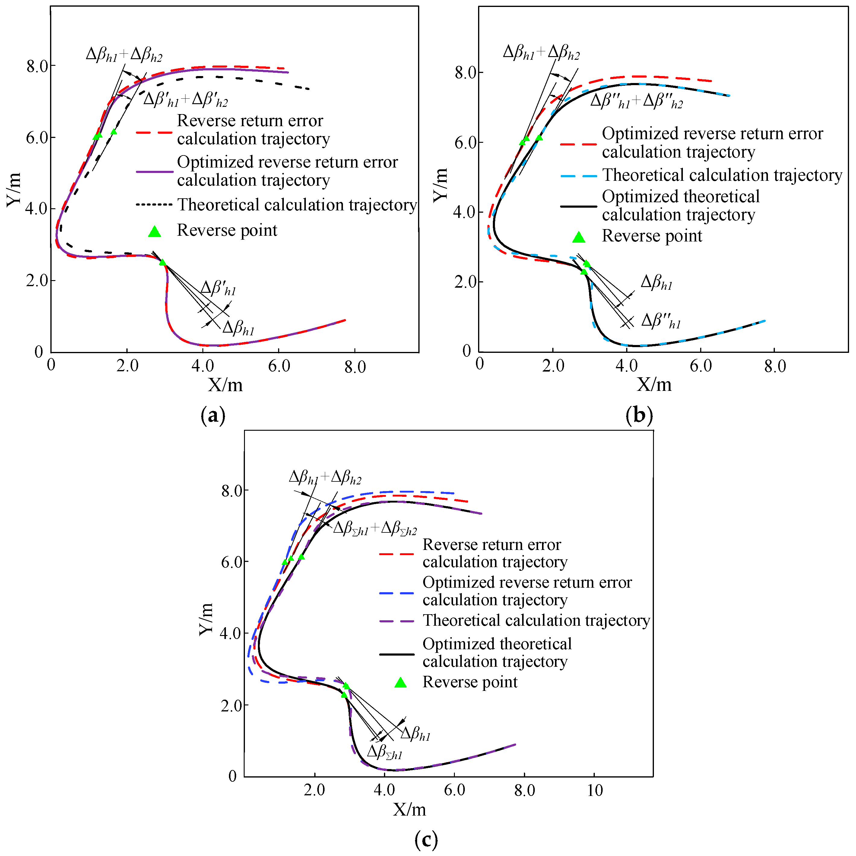
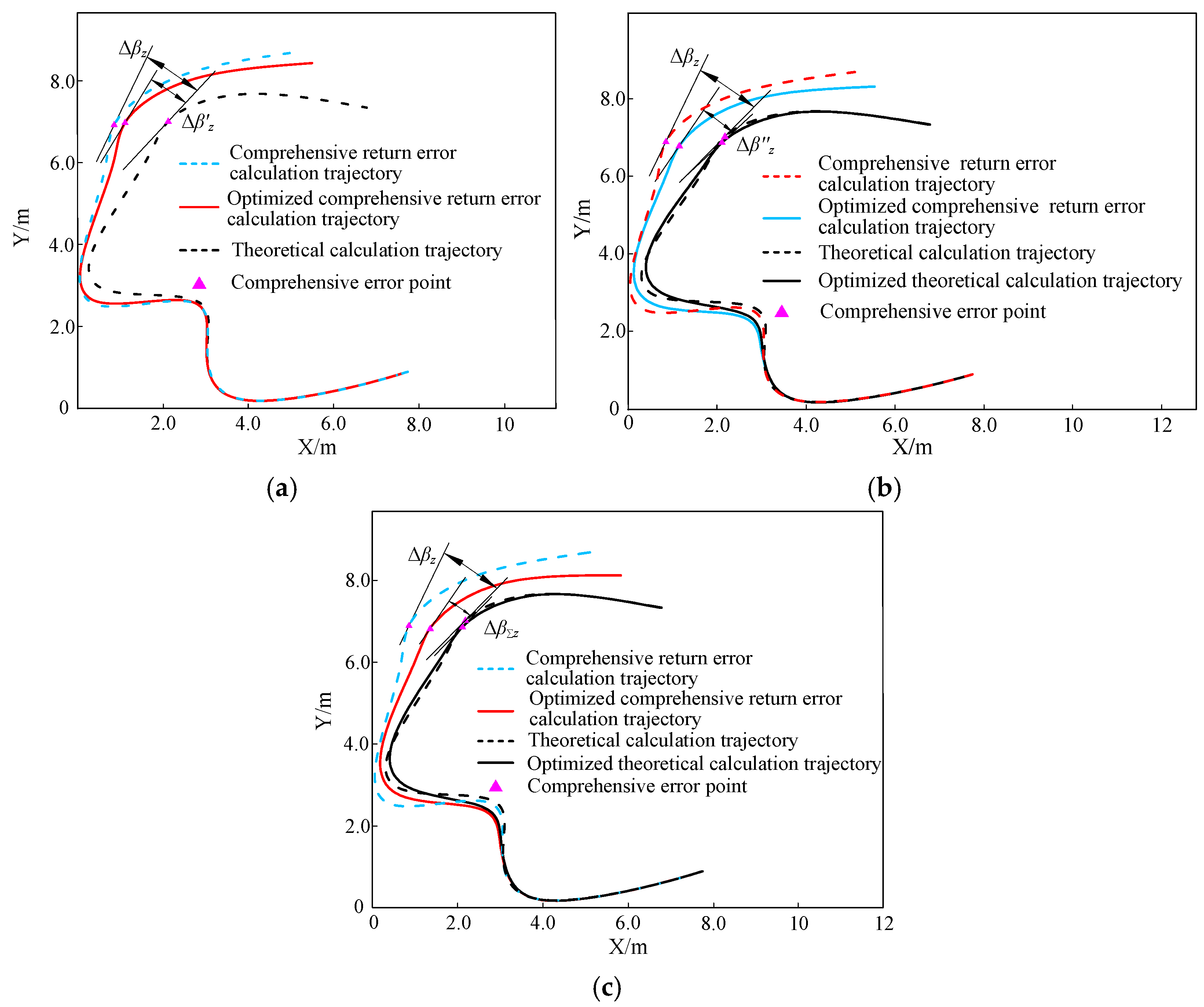
The calculated trajectories generated in MATLAB (Code Location: Appendix A) using the pre- and post-optimization return error of gear transmissions enabled a clear visual comparison of the optimization effects. After adjusting the transmission ratio, the return error of gear transmission decreased, leading to a corresponding reduction in trajectory deviation, as shown in Figure 18a. Following cam optimization, the peak value of the push stroke was reduced, thereby weakening the correlation between jump deflection error and push stroke. This modification mitigated the influence of the return error of the gear transmission on steering accuracy, as illustrated in Figure 18b. By integrating both strategies, the return error of gear transmission and its associated deflection error were simultaneously reduced. The overall improvement is demonstrated in Figure 18c.

The calculation trajectories post-optimization of the transmission ratio, cam contour curve, and comprehensive optimization are presented in Figure 19a, Figure 19b, and Figure 19c, respectively, with optimization principles as described earlier.

The combined influence of both return error of gear transmissions results in a decreased actual right-turn amplitude of the car, while the left-turn amplitude increases, leading to a significant leftward deviation in the calculation trajectory. By combining the optimization strategies of adjusting the transmission ratio and optimizing the cam profile, the trajectory calculation of the vehicle was carried out. The calculation trajectories are shown in Figure 20a, Figure 20b, and Figure 20c, respectively.

From the calculation results, it is evident that, compared to the theoretical trajectory, the calculation trajectory affected by the return error of the gear transmission exhibits a more pronounced leftward offset. Through transmission ratio adjustment and cam profile optimization, the steering accuracy of the mechanism was considerably improved, leading to a 45.31% enhancement in overall performance.

5. Physical Production Test

To verify the conclusion’s feasibility, a series of experiments is conducted using a carbon-free car. The carbon-free car used in the experiment is shown in Figure 21. The experiment employs traditional mechanical design principles along with modern technical methods. The test involves precise control of the motor rotation duration via an STM32 series microcontroller (Manufacturer: Guangzhou Xingyi Electronic Technology Co., Ltd., Guangzhou, China), and employs an LM320B series high-precision electronic digital inclinometer (Manufacturer: UNI-TREND TECHNOLOGY (CHINA) CO., LTD., Dongguang, China) to measure the cam rotation angle; its measurement accuracy is 0.01°. Following data acquisition, the normal distribution is employed to calculate the mean, variance, confidence intervals, and other statistical measures. The specific experimental design details are presented below.

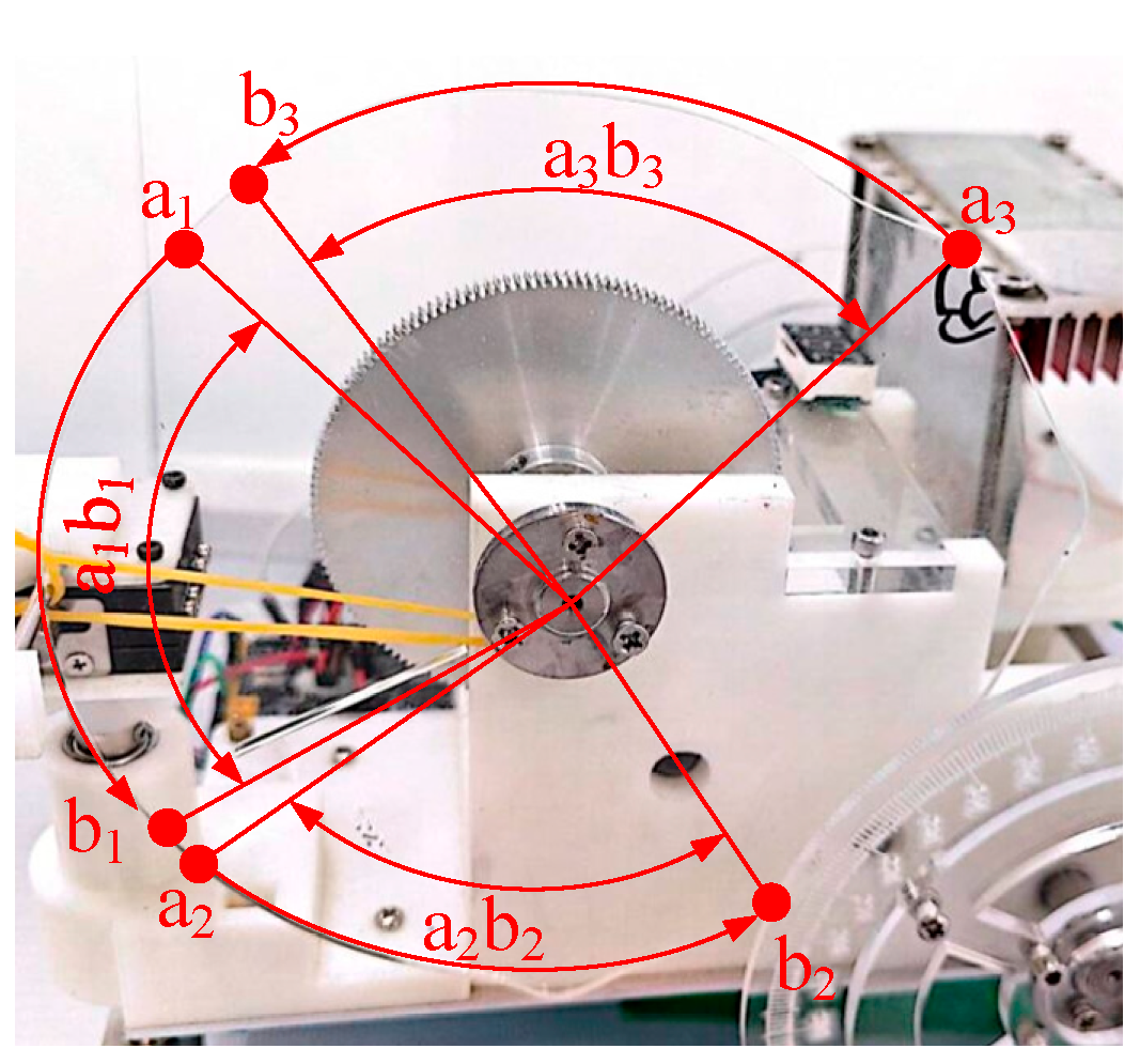
A car free of carbon emissions is operated by a small DC motor, which rotates at 60 revolutions per minute. The total transmission ratio for the three-stage gear set is designated as $\mathrm{i}$ = 45. The experiment was divided into three groups to test the cam’s smooth zone, jumping zone, and turning zone, respectively. Each group underwent 100 trials lasting 15 s each, and the average value was calculated to minimize experimental error. A controlled variable approach was adopted to mitigate the influence of factors such as motor speed deviation, vibration, and assembly inaccuracies on the carbon-free car, with the control group defined by the cam rotation angle in the smooth zone over a 15 s interval. For each test, the initial and final contact points between the cam and follower were recorded as points a₁–a₃ and b₁–b₃, corresponding to the three profile segments. The rotation angle of each segment (a₁b₁, a₂b₂, a₃b₃) was measured using a high-precision digital inclinometer. The principle of the experiment is shown in Figure 22.

A 95% confidence interval was calculated using the standard deviation of the experimental data and the normal distribution. The normal distribution probability density function is defined as follows [38]:

$$f\left(x\right)={\displaystyle \frac{1}{\sqrt{2\pi \sigma }}}{e}^{-{\displaystyle \frac{{\left(x-\mu \right)}^2}{2{\sigma }^2}}}$$

(31)

$$\sigma =\sqrt{{\displaystyle \frac{\left[{\left(x_1-\overline{X}\right)}^2+{\left(x_2-\overline{X}\right)}^2+\cdots +{\left(x_n-\overline{X}\right)}^2\right]}{n}}}$$

(32)

$$(\overline{X}-{\displaystyle \frac{\sigma }{\sqrt{n}}}·u_{{\displaystyle \frac{1-0.95}{2}}},\overline{X}+{\displaystyle \frac{\sigma }{\sqrt{n}}}·u_{{\displaystyle \frac{1-0.95}{2}}})$$

(33)

where n represents the number of experimental data, which is 100, μ represents the mathematical expectation, σ represents the standard deviation, $\overline{X}$ represents the average value, u is the critical value of the normal distribution, and $u_{\frac{1-0.95}{2}}$ can be obtained by referring to the table of u values of the normal distribution, which is 1.96.

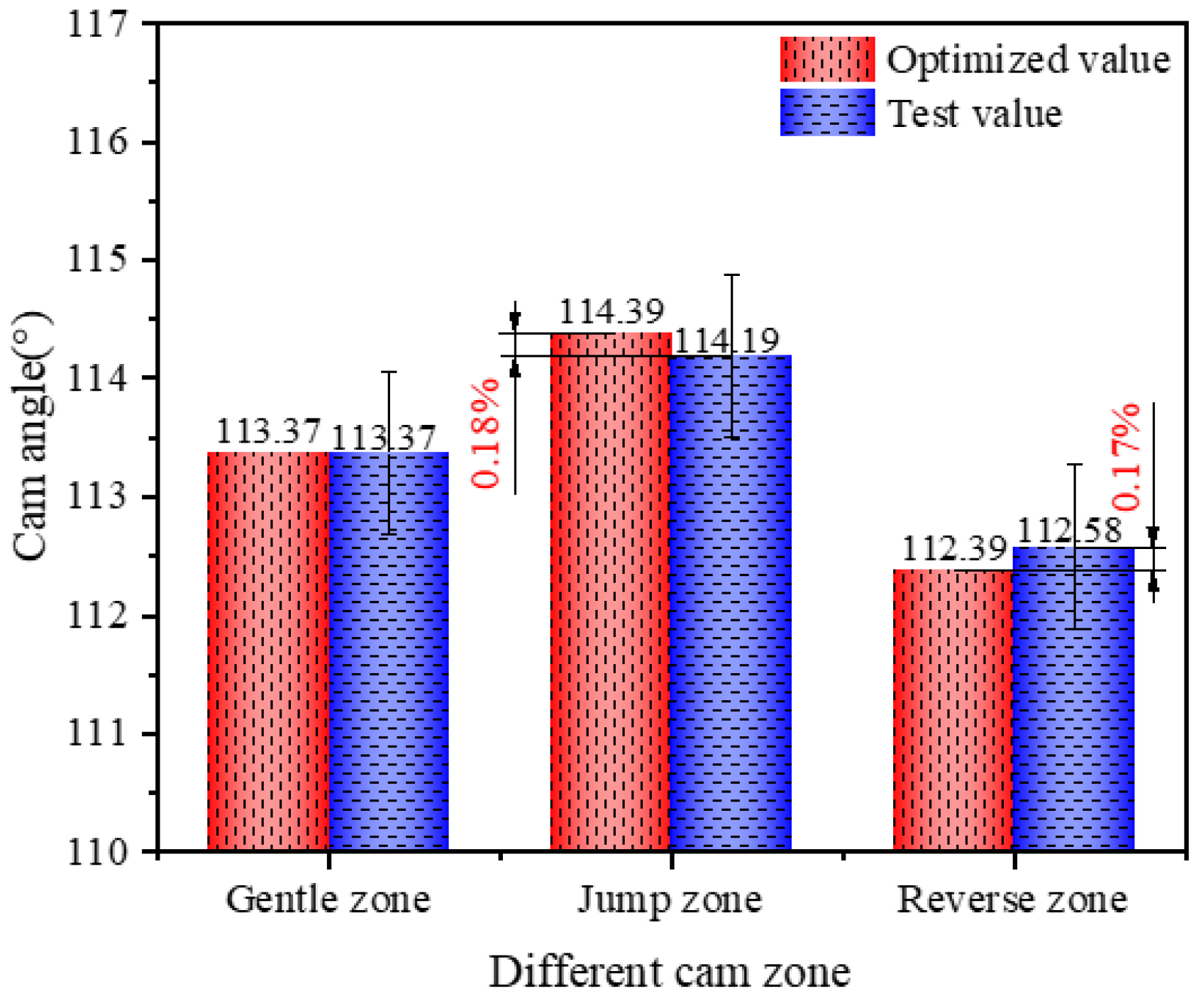
The average values obtained from the three sets of test data are 113.37, 114.19, and 112.58, respectively. According to Equation (32), it is calculated that the standard deviations of the three groups of experimental data were 0.68, 0.68, and 0.69, respectively. When the standard deviation is known, the confidence interval with a 95% confidence level can be calculated using Equation (33). The corresponding confidence intervals were [113.24, 113.50], [114.06, 114.32], and [112.45, 112.71].

Based on the above calculation results, Figure 23 compares the average values of the angles obtained from the three groups of experiments with the optimized results. There is no difference in the gentle zone, while the differences in the jump zone and the reverse zone are 0.18% and 0.17%, respectively. The experimental findings validate that the jump return error of gear transmission and the reverse return error of gear transmission are authentic and approximate the values predicted by theoretical calculations.

6. Conclusions

This study investigated the cam steering mechanism in a carbon-free vehicle. Through theoretical modeling and MATLAB-based numerical analysis, the influence of gear transmission backlash on steering accuracy is evaluated. Furthermore, the cam profile and gear transmission ratio are optimized to mitigate the impact of backlash on the cam mechanism’s performance. The main conclusions of this work are summarized as follows:

(1)

The analysis of car motion facilitated the derivation of design and trajectory calculation concepts for the cam, and the construction of a mathematical model for gear return error of gear transmission, considering factors such as center distance and tooth thickness deviation. This foundation supports subsequent calculation and optimization efforts.

(2)

The comprehensive return error of gear transmission exhibits a negative correlation with the rear transmission ratio, while the deflection error induced by the return error of gear transmission shows a positive correlation with the peak and valley values of the push stroke. Consequently, a method to increase the rear transmission ratio and optimize the cam profile curve is proposed, aiming to diminish the impact of the return error of gear transmission on the steering accuracy of the car. The optimization results show that the deflection errors are reduced by 24.74% and 27.15%, respectively. Furthermore, comprehensive optimization resulted in a 45.31% reduction in cumulative deflection error.

(3)

The trajectory was calculated using MATLAB 2023b, which incorporated the return error of the gear transmission both before and after optimization. This analysis helped quantify the impact of the return error of gear transmission on the car’s trajectory, thereby corroborating the theoretical soundness of the optimization method. The validity of these findings was further confirmed through the construction and testing of a physical prototype. This study provides critical insights for the design, manufacturing, and trajectory calibration of equipment with complex motion paths. Beyond this, the proposed optimization method offers technical support for achieving precise motion control in broader applications requiring complex trajectories, such as in advanced machining and robotic guidance within automated production lines, thereby paving the way for its adoption in these fields.

References

1. Cheng, Z.; Yang, J.; Sun, J.; Zhao, L. Trajectory Planning of Unmanned Aerial Vehicles in Complex Environments Based on Intelligent Algorithm. Drones 2025, 9, 468. [Google Scholar] [CrossRef] [Scilit]
2. Han, Z.; Tian, M.; Gongye, Z.; Xue, D.; Xing, J.; Wang, Q.; Gao, Y.; Wang, J.; Xu, C.; Gao, F. Hierarchically depicting vehicle trajectory with stability in complex environments. Sci. Robot. 2025, 10, 4551. [Google Scholar] [CrossRef] [Scilit]
3. Gong, L.; Li, L.; Zhang, L.; Zhang, B.; Zheng, D.; Li, N. Pseudo-random and dynamic selective trajectories generation for mid-spatial frequency error rapid convergence. Precis. Eng. 2025, 97, 572–594. [Google Scholar] [CrossRef] [Scilit]
4. Liu, L.; Sun, M.; Zhao, E.; Zhu, K. Three-Dimensional Dynamic Trajectory Planning for Autonomous Underwater Robots Under the PPO-IIFDS Framework. J. Mar. Sci. Eng. 2025, 13, 445. [Google Scholar] [CrossRef] [Scilit]
5. Chen, G.; Yuan, S.; Zhang, Z.; Liang, X. Multi-UAV collaborative trajectory planning for non-cooperative target tracking in complex environment. Proc. Inst. Mech. Eng. Part G J. Aerosp. Eng. 2025, 239, 1423–1439. [Google Scholar] [CrossRef] [Scilit]
6. Bi, G.; Lu, L.; Zhang, L.; Fan, C.; Sun, L. High-precision trajectory calibration for robot surface machining by meta-heuristic search algorithm from local error in machining area. Int. J. Adv. Manuf. Technol. 2025, 138, 2281–2295. [Google Scholar] [CrossRef] [Scilit]
7. Ma, X.; Wang, X.; Zhang, H.; Li, H. The teaching application of the backward design method in Chinese national undergraduate engineering training integration ability competition: Take the double 8 carbon-free car as an example. Appl. Sci. 2023, 13, 8829. [Google Scholar] [CrossRef] [Scilit]
8. Wang, H.; Shang, L.; Tang, D.; Li, Z. Research themes, evolution trends, and future challenges in China’s carbon emission studies. Sustainability 2024, 16, 2080. [Google Scholar] [CrossRef] [Scilit]
9. He, R.H.; Xiao, J.C.; Du, K.Q.; Yue, J.H.; Lan, M.H. Structural Design and Analysis of S-Ring Carbon-Free Cars. J. Mach. Des. 2023, 40, 48–54. [Google Scholar]
10. Chen, Y.N.; Hsu, K.L. Necessary and Sufficient Design Conditions for Overconstrained Cam Mechanisms With Flat-Faced and Roller Follower. J. Mech. Robot. 2025, 17, 075002. [Google Scholar] [CrossRef] [Scilit]
11. Català, P.; Veciana, J.M.; Jordi, L. Energy loss comparison between kinematically equivalent mechanisms: Slider-crank and eccentric cam. Mech. Based Des. Struct. Mach. 2024, 52, 9435–9457. [Google Scholar] [CrossRef] [Scilit]
12. Merticaru, E.; Merticaru, V.; Nagîț, G.; Mihalache, A.M.; Tăbăcaru, L.L.; Rîpanu, M.I. Analytical, numerical and experimental analysis of a positive displacement cam mechanism—A case study. Machines 2023, 11, 770. [Google Scholar] [CrossRef] [Scilit]
13. Iriarte, X.; Bacaicoa, J.; Plaza, A.; Aginaga, J. A unified analytical disk cam profile generation methodology using the Instantaneous Center of Rotation for educational purpose. Mech. Mach. Theory 2024, 196, 105625. [Google Scholar] [CrossRef] [Scilit]
14. Zhou, C.; Hu, B.; Chen, S.; Ma, L. Design and analysis of high-speed cam mechanism using Fourier series. Mech. Mach. Theory 2016, 104, 118–129. [Google Scholar] [CrossRef] [Scilit]
15. Pozo-Palacios, J.; Fulbright, N.J.; Voth, J.A.; Van de Ven, J.D. Comparison of forward and inverse cam generation methods for the design of cam-linkage mechanisms. Mech. Mach. Theory 2023, 190, 105465. [Google Scholar] [CrossRef] [Scilit]
16. Lan, W.; Fan, S.; Fan, S. Analysis of structural design defects in parallel overloading mechanisms with cam transmission mechanism. Appl. Math. Model. 2022, 107, 717–739. [Google Scholar] [CrossRef] [Scilit]
17. Yang, Y.; Xie, R.; Wang, J.; Tao, S. Design of a novel coaxial cam-linkage indexing mechanism. Mech. Mach. Theory 2022, 169, 104681. [Google Scholar] [CrossRef] [Scilit]
18. Zheng, X.; Zhao, H.; Zhang, S.; Liu, D.; Wang, B. Design Method of Cam Steering Mechanism Based on Path Fitting. Processes 2024, 12, 1037. [Google Scholar] [CrossRef] [Scilit]
19. Wang, C.; Peng, W. Optimization design for reliability of the oscillating follower disk cam mechanism based on improved hunter-prey optimization algorithm. IEEE Access 2024, 12, 182532–182546. [Google Scholar] [CrossRef] [Scilit]
20. Zhu, G.; Wang, Y.; Zhu, G.-N.; Weng, M.; Liu, J.; Zhou, J.; Lu, B. Parameter optimization of large-size high-speed cam-linkage mechanism for kinematic performance. Actuators 2022, 12, 2. [Google Scholar] [CrossRef] [Scilit]
21. Kang, Y.-H.; Huang, H.-C.; Yang, B.-Y. Optimal design and dynamic analysis of a spring-actuated cam-linkage mechanism in a vacuum circuit breaker. Machines 2023, 11, 150. [Google Scholar] [CrossRef] [Scilit]
22. Li, M.; Liang, R.; Zhang, Y.; Peng, C.; Mu, D.; Wan, Z. On-line measurement method of transmission backlash based on angular velocity and double-end angular position information. Meas. Control 2021, 54, 65–72. [Google Scholar] [CrossRef] [Scilit]
23. Wang, J.; Wu, Z.; Wang, H.; Ding, J.; Yi, C. Analysis of influence of thermal tooth backlash on nonlinear dynamic characteristics of planetary gear system. Nonlinear Dyn. 2025, 113, 289–311. [Google Scholar] [CrossRef] [Scilit]
24. Tian, G.; Gao, Z.; Liu, P.; Bian, Y. Dynamic modeling and stability analysis for a spur gear system considering gear backlash and bearing clearance. Machines 2022, 10, 439. [Google Scholar] [CrossRef] [Scilit]
25. Zenn, W.; Herold, S.; Melz, T. Estimation of the backlash size on rack-and-pinion drives of machine tools using supervised learning classification methods. Int. J. Adv. Manuf. Technol. 2025, 137, 5279–5292. [Google Scholar] [CrossRef] [Scilit]
26. Reddy, P.; Shahbakhti, M.; Ravichandran, M.; Doering, J. Real-time estimation of backlash size in automotive drivetrains. IEEE/ASME Trans. Mechatron. 2022, 27, 3362–3372. [Google Scholar] [CrossRef] [Scilit]
27. Ma, X.-T.; Zhang, H.; Zhang, H.; Wang, X.F.; Zhu, Z. Research on reverse design method of S-ring carbon-free car. Machinery 2022, 49, 23–28. [Google Scholar]
28. Fang, L.; Wu, Y.; Mou, Z.; Guo, Y. Reverse calculation analysis and design of cam of carbon free car with “8” trajectory. J. Mach. Des. 2023, 40, 106–111. [Google Scholar]
29. Sun, Q.; Cui, Y.; Li, P.; Zhang, Z.; Li, W. Design of “8” potential energy driven vehicle based on MATLAB calculation. Sci. Technol. Innov. 2022, 25, 167–170. [Google Scholar]
30. Song, C.; Wang, S.; Li, X.; Zhu, C.; Yang, Y. Influences of circular runout errors and processing parameters for slotting on the accuracy of harmonic reducer. J. Adv. Mech. Des. Syst. Manuf. 2022, 16, JAMDSM0003. [Google Scholar] [CrossRef] [Scilit]
31. Wang, H.; Zhang, X.; Fang, K.; Qiu, Y.; Zhang, Z. Return error simulation analysis and experimental study for RV reducer with ADAMS. J. Adv. Mech. Des. Syst. Manuf. 2024, 18, JAMDSM0023. [Google Scholar] [CrossRef] [Scilit]
32. Wen, B. Mechanical Design Handbook; Machinery Industry Press: Beijing, China, 2018. [Google Scholar]
33. Zhang, L.; Fan, Y. Analysis on Influence of Gear Backlash on Gear Transmission Accuracy. Mach. Tool Hydraul. 2017, 45, 114–116. [Google Scholar]
34. Li, J. Trajectory and structural design of carbon free car based on B-spline curve. J. Mach. Des. 2023, 40, 114–118. [Google Scholar]
35. Li, J. Universal design method of carbon-free car based on 3D motion calculation. J. Mach. Des. 2022, 38, 46–48+52. [Google Scholar]
36. Yu, J.; Huang, K.; Luo, H.; Wu, Y.; Long, X. Manipulate optimal high-order motion parameters to construct high-speed cam curve with optimized dynamic performance. Appl. Math. Comput. 2020, 371, 124953. [Google Scholar] [CrossRef] [Scilit]
37. Zhang, K.; Xiu, F.; Zhang, Y.; Su, L.; Yang, X. Design of double 8-shaped trajectory carbon-free car based on cam mechanism. J. Mach. Des. 2020, 37, 24–28. [Google Scholar] [CrossRef]
38. Gong, G. Probability Theory and Mathematical Statistics; Tsinghua University Press Co., Ltd.: Beijing, China, 2006. [Google Scholar]
Figure 1. Three-dimensional rendering of carbon-free car.
Machines 13 01075 g001
Figure 2. The fine adjustment mechanism.
Machines 13 01075 g002
Figure 3. Operation flowchart.
Machines 13 01075 g003
Figure 4. Simplified diagram of the car mechanism. (a) Left turn status and (b) right turn status.
Machines 13 01075 g004
Figure 5. Profile curve of cam.
Machines 13 01075 g005
Figure 6. Comparison of the calculated trajectory with the original trajectory.
Machines 13 01075 g006
Figure 7. Cam force. (a) Normal meshing state and (b) abnormal meshing state.
Machines 13 01075 g007
Figure 8. Jumping motion of cam follower.
Machines 13 01075 g008
Figure 9. Jump deflection error and reverse deflection error of cam follower.
Machines 13 01075 g009
Figure 10. The trajectory of the car before optimization. (a) Considering only the jump return error of gear transmission, (b) considering only the reverse return error of gear transmission, and (c) considering jump return and reverse return error of gear transmissions.
Machines 13 01075 g010
Figure 11. Flowchart of the optimization process.
Machines 13 01075 g011
Figure 12. The deflection error after optimizing the transmission ratio.
Machines 13 01075 g012
Figure 13. Comparison of deflection error after optimization of transmission ratio with the original deflection error.
Machines 13 01075 g013
Figure 14. Comparison of the stroke after optimizing the cam profile with the original stroke.
Machines 13 01075 g014
Figure 15. Comparison of the deflection angle error after optimizing the cam profile with the original deflection angle error.
Machines 13 01075 g015
Figure 16. Comparison of cumulative errors after optimizing the cam profile with the original cumulative errors. (a) Stroke. (b) Deflection angle.
Machines 13 01075 g016
Figure 17. Comparison of optimized comprehensive deflection error with the original deflection error.
Machines 13 01075 g017
Figure 18. Trajectory of car with jump return error of gear transmission. (a) Transmission ratio optimization. (b) Cam optimization. (c) Comprehensive optimization.
Machines 13 01075 g018
Figure 19. Trajectory of car with reverse return error of gear transmission. (a) Transmission ratio optimization. (b) Cam optimization. (c) Comprehensive optimization.
Machines 13 01075 g019
Figure 20. Trajectory of car with comprehensive return error of gear transmission. (a) Transmission ratio optimization. (b) Cam optimization. (c) Comprehensive optimization.
Machines 13 01075 g020
Figure 21. Test site setup and physical model of the carbon-free car.
Machines 13 01075 g021
Figure 22. Principle of the experiment.
Machines 13 01075 g022
Figure 23. Cam angle optimization and experimental comparison.
Machines 13 01075 g023