Article

The Diagnosis and Recovery of Faults in the Workshop Environmental Control System Sensor Network Based on Medium-to-Long-Term Predictions

Key Lab of Modern Manufacture Quality Engineering, Hubei University of Technology, Wuhan 430068, China
*
Author to whom correspondence should be addressed.
Machines 2025, 13(11), 975; https://doi.org/10.3390/machines13110975
Submission received: 10 September 2025 / Revised: 15 October 2025 / Accepted: 21 October 2025 / Published: 22 October 2025
(This article belongs to the Section Machines Testing and Maintenance)

Abstract

For the fault issues in the workshop environmental control system sensor network, a fault diagnosis and recovery method based on medium-to-long-term predictions is proposed. Firstly, a temperature observer based on the Informer model is established. Then, the predicted data temporarily replaces the missing real data, and the model predicts the state of the sensor system within the step size. Secondly, the predicted data is combined with the measured temperature series, and residuals are utilized for real-time detection of sensor faults. Finally, the predicted data at the time of the fault replaces the real data, enabling the recovery of fault data; experiments are conducted to verify the effectiveness of the proposed method. The results indicate that when the prediction horizon is 1, 5, 10, 20, and 50, the average fault diagnosis rates under four fault levels are 94.40%, 95.28%, 94.79%, 92.52%, and 93.35%, respectively. The average coefficients of determination for data recovery are 0.999, 0.997, 0.995, 0.985, and 0.915, respectively. This achieves medium-to-long-term predictions in the field of sensor fault diagnosis.

1. Introduction

A large amount of precision equipment is continuously being deployed, placing higher demands on workshop environmental control systems [1,2]. The sensor network, serving as a critical component within the workshop’s environmental control system, undertakes the vital task of environmental information acquisition, and its reliability directly impacts the performance and stability of the entire system [3]. The application of sensors in the workshop environmental control system is particularly crucial, as they are responsible for monitoring and feeding back key parameters of the system, playing a vital role in ensuring the normal operation of the environmental control system [4,5]. Therefore, research on fault diagnosis and recovery for sensor networks in workshop environmental control systems is highly significant for promoting the advancement of smart manufacturing.
In recent years, many scholars have carried out many innovative studies on fault diagnosis techniques within environmental control systems. Data-driven methods do not require the establishment of mathematical models; they utilize operational data from environmental control systems for fault diagnosis. Methods included are Support Vector Machines (SVM) [6,7], Principal Component Analysis (PCA) [8,9], and deep learning-based approaches [10], among others.
Gins et al. [11] consider the application of classification algorithms for data-driven fault diagnosis of batch processes. Classification-based methods often require a large amount of fault data to train models, whereas industrial databases typically lack sufficient fault data [12]. However, prediction models do not require fault data; instead, they use only historical normal operating data to complete fault diagnosis. Li et al. [13] propose an improved Bayesian method that combines principal component analysis and an improved Bayesian network, using a predictive approach to diagnose sensor faults in Heating Ventilation and Air Conditioning (HVAC) systems. The aforementioned methods perform well in single-step prediction tasks but are poor at long-sequence time series prediction tasks. As the demand for long-term stable system performance increases, medium- and long-term prediction has become a key task for sensor network fault diagnosis in environmental control systems.
By analyzing the historical time series collected by sensors to predict the time series of sensors for a relatively long time in the future, this task is known as the long-sequence time prediction task [14]. The Informer model, as a new Transformer-based sequence modeling method, has emerged in the field of long-sequence time series prediction with its efficient and accurate performance [15]. Guo et al. [16] develop a stacked Informer model for predicting power line trip faults, enhancing the accuracy of fault sequence prediction. Klimek et al. and Xu et al. [17,18] propose a sparse attention mechanism based on the Informer model, which improves prediction capability to some extent. Therefore, the advantages of the Informer model in long sequence time prediction are leveraged to address the fault domain within workshop environmental control system sensor networks in this article, thereby enhancing the long-term stability of system performance.
In this investigation, a fault diagnosis and recovery method for the sensor network of a workshop environmental control system based on medium- and long-term predictions is proposed. The method is composed of three parts: state prediction, fault diagnosis, and fault recovery, achieving real-time detection of faults in the sensor network and recovery of fault data. The effectiveness of the method is verified through experiments.

2. The Framework for Fault Diagnosis and Recovery

A fault diagnosis and recovery method for the sensor network of the workshop environmental control system is proposed based on medium-to-long-term forecasting. To implement this method, several key issues must be addressed: Long sequence prediction generation: Predictive sensor sequences must be generated by the model. Fault diagnosis: After the actual values are acquired, the residual between the predicted values and the measured values for each sensor is calculated. Fault localization: Faulty data points within the sensor network must be accurately located. Fault data recovery: Faulty data is recovered by utilizing the predicted data output from the Informer model to overwrite the fault data. This ensures the environmental control system can be maintained for short-term operation.
(1)
Data Preprocessing: Missing data are initially filled using a one-dimensional interpolation method, followed by the elimination of unstable data points. Exponential Weighted Moving Average (EWMA) is employed for noise reduction in the acquired data to enhance data quality. Subsequently, the data are normalized to mitigate the influence of varying scales. For the experiment, the data are partitioned into training, testing, and validation sets. The training set is utilized to train the Informer model; the testing set is used to determine the fault threshold; and the validation set is employed for conducting fault diagnosis trials.
(2)
Construction of Multivariate Input Medium-to-Long-Term Prediction Model: The preprocessed data are fed into the encoder of the Informer model. Within the encoder, critical features are extracted from the data via a sparse self-attention mechanism, capturing long-term dependencies within the time series and spatial correlations among different sensors. Subsequently, these extracted features are utilized by the decoder, which predicts the entire future time series through a generative decoding mechanism. During model construction, Mean Squared Error (MSE) is adopted as the loss function, and early stopping is implemented to prevent overfitting.
(3)
State Prediction: Based on the sensor prediction sequences, these predicted values are utilized as temporary references during the current system operation. This enables the future state of sensors to be anticipated in advance, thereby preventing system failures caused by state delays or unexpected events.
(4)
Fault Threshold Analysis: The residual sequences between the outputs of the diagnostic soft sensors and the physical sensors on the testing set are calculated. The method described in Section 3.2 is then applied to determine the fault threshold based on these residuals.
(5)
Fault Diagnosis: Fault diagnosis is performed by applying the criterion of consecutive exceedances. A data point is identified as faulty when the residuals of a sensor exceed the fault threshold continuously for five consecutive instances.
(6)
Fault Data Recovery: Following the identification of faulty data points within a sensor, the predicted values output by the fault diagnosis model are employed to overwrite the faulty values. The predicted values are thus substituted for the faulty ones during the diagnostic process, achieving fault data recovery.

3. A Long-Term Predictive Fault Diagnosis Model for the Sensor Network in the Workshop Environmental Control System

3.1. Long Sequence Prediction Model Informer

The Informer model is designed specifically for long-sequence time-series forecasting, with its core lying in a unique attention mechanism. Compared to the traditional Transformer model, three distinct features are exhibited by the Informer model. Firstly, the ProbSparse self-attention mechanism is employed by the Informer. This mechanism is achieved at O(LlogL) levels in terms of time complexity and memory usage, allowing long-term dependencies within sequences to be efficiently captured, and a significant improvement in computational complexity is realized. Secondly, through the self-attention distillation technique, extremely long input sequences can be effectively handled by the Informer, leading to enhanced model processing capability and efficiency. Finally, a generative-style decoder is adopted by the Informer model. This enables the entire long time-series to be predicted in a single forward pass, rather than being predicted step by step, significantly increasing the efficiency and speed of the prediction process. The Informer model is composed of two main parts: an encoder and a decoder. Input time series are transformed into a fixed-length representation by the encoder. Predictions are then generated by the decoder based on this representation.
(1)
Informer Model Input
The primary input to the Informer model consists of a time series. After determining the input window size, the model input at each time point is represented as in Equation (1).
X t = x 1 t , x 2 t , x i t
where i represents the length of the current input sequence, and the predicted sequence output at time step t is as shown in Equation (2).
Y t = y 1 t , y 2 t , y j t
where j represents the length of the predicted sequence output by the model at time t.
(2)
Probability Sparse Self-Attention Mechanism
Scale the dot product of the Query vector, Key vector, and Value vector of the traditional self-attention mechanism, as shown in Equation (3).
A t t e n t i o n ( Q , K , V ) = S o f t m a x Q K T d V
where Q R L Q × d represents the Query vector, K R L K × d represents the Key vector, and V R L V × d represents the Value vector, with d being the input dimension.
The attention for the i-th Query vector is as shown in Equation (4).
A t t e n t i o n q i , K , V = j k q i , k j l k q i , k l v j = E p k j q i v j
Self-attention probability scores exhibit sparse characteristics and a long-tail distribution, which means only a few attention scores have high values—and it is precisely these high-value scores that contribute most significantly to the overall attention. Therefore, one may consider ignoring the parts with smaller weights, thereby avoiding the calculation of the contribution of Query vectors with smaller influence on the Value vectors. The sparsity evaluation formula for Query vectors is as shown in Equation (5).
M q i , K = l n j = 1 L K e q i k j T d 1 L K j = 1 L K q i k j T d
where the first term on the right side represents taking the maximum value for each Key component, and the second term is the calculation of the arithmetic mean.
Based on the above evaluation formula, the mathematical expression for ProbSparse self-attention is as shown in Equation (6).
A t t e n t i o n Q , K , V = S o f t m a x Q ¯ K T d V
where Q ¯ is a sparse matrix of the same size as q , and it only exists in the components of Queries with ranks among the top u according to the sparsity evaluation metric M (q, K).
The u is determined by the sampling coefficient c , as shown in Equation (7).
u = c · l n L Q
Therefore, in sparse self-attention, only the dot product needs to be calculated for each Query–Key component, significantly reducing memory overhead and improving computational efficiency.
(3)
Encoder
The encoder employs a multi-scale time encoder structure. This structure enables the model to consider information across different time scales simultaneously, thereby better capturing long-range dependencies in the sequence. The feature mapping in the encoder does not contain redundant information about Value; instead, it only includes Value vectors corresponding to Key–Value pairs with higher attention scores. Additionally, the encoder utilizes distillation techniques to reinforce dominant features, allowing for greater focus in the subsequent layer of sparse self-attention. During this process, the model’s input is continuously reduced, and the specific distillation operation is as shown in Equation (8).
X j + 1 t = M a x P o o l ( E L U ( C o n v l d ( X j t A B ) ) )
where [Xtj]AB includes multi-head probabilistic sparse self-attention and key operations within the attention blocks. Convld applies a one-dimensional convolution along the time dimension using the ELU activation function, followed by a max pooling layer that reduces the sample size to half its original length. To enhance the model’s robustness, the encoder is stacked and its outputs are concatenated to obtain the final encoder output, enabling the processing of longer input sequences.
(4)
Decoder
The decoder employs a generative decoder design. Unlike traditional step-by-step prediction methods, the generative decoder predicts the entire long sequence at once, significantly improving the inference speed for long sequence predictions. The decoder’s input vector is as shown in Equation (9).
X f e e d _ d e t = C o n c a t ( X t o k e n t , X O t ) R ( L l a b e l + L y ) × d m o d e l
where X t o k e n t is a subsequence of length L l a b e l selected from the input sequence as a label, which means a labeled sequence is added before the formal prediction sequence. X O t is a placeholder that constitutes the overall target sequence, set to 0. Finally, a fully connected layer is used to obtain the model output, which can be used for univariate or multivariate prediction.

3.2. Sensor System State Prediction

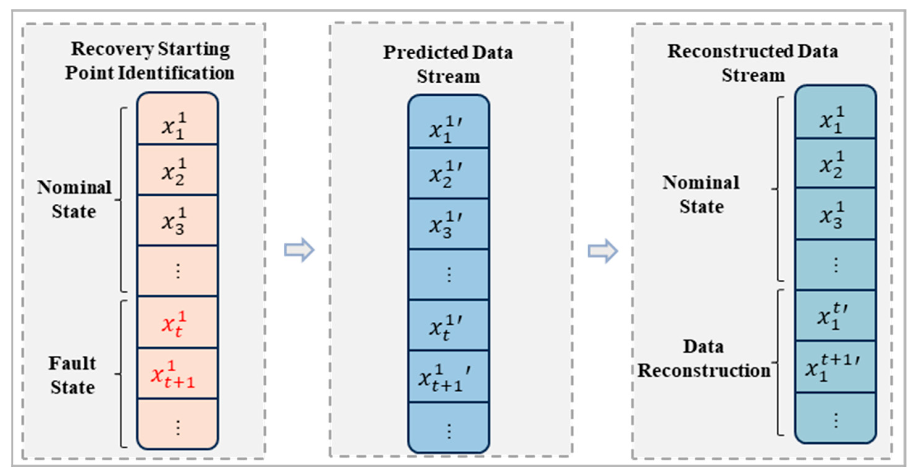
After obtaining the predicted sequence from the sensor, since the actual values are not yet available, the predicted values are temporarily substituted for the actual values and passed to the downstream system. This process utilizes the long-term sequence predictions generated by the Informer model to predict the status of the sensor network in the workshop environmental control system. This ensures the continuous operation of the system within the prediction period and helps prevent potential failures. By predicting the sensor data in advance, the system maintains stable operation even without actual data input. The principle is illustrated in Figure 1.

3.3. Fault Threshold Analysis

A subset is identified within the dataset for determining the fault thresholds. The residual vector of the i-th training sample at time t is given by Equation (10).
ε t t r , i = x t i ^ x t i
where x t i ^ is the time series of predicted values output by the prediction model at time t, x t i is the sensor time series at the t-th sampling time instant, and the vector is represented as in Equation (11).
x t i = x t , 1 i , x t , 2 i , x t , N i T R N
where N is the number of sensors.
The i-th threshold determines the reconstruction residual vector of the sample at time t, as shown in Equation (12).
ε t t e , i = ε t , 1 t e , i , ε t , 2 t e , i , ε t , j t e , i ε t , N t e , i T
where ε t , j t e , i is the reconstruction residual value of the j-th sensor at the t-th sampling instant, determined by the i-th threshold for the sample. The expression for the fault threshold ε j of the j-th sensor is given in Equation (13).
ε j = m a x ε t , j t e , i
where Nte is the number of samples in the sample set for threshold determination, and 1 ≤ I ≤ Nte, 1 ≤ tT. The fault threshold vector ε t e , u is composed of the fault thresholds of the N sensors, and its expression is given in Equation (14).
ε t e , u = ε 1 , ε 2 , ε N T

3.4. Residual-Based Sensor Fault Diagnosis

In the dataset, a validation set sample is partitioned, and different-sized bias faults are injected into each sensor. The reconstruction residual vector of the i-th test sample at time t is given by Equation (15).
ε t v a , i = ε t , 1 v a , i , ε t , 2 v a , i , ε t , j v a , i ε t , N v a , i T
where ε t , j v a , i is the residual value of the j-th sensor in the i-th test sample at time t.
For each sampling instance within the test sample, its reconstruction residual vector is compared element-wise with the corresponding entries in the fault threshold vector ε v a , u to identify the sensors experiencing faults. The criterion for determining a faulty sensor is as provided in Equation (16).
ε t , j v a , i > ε j ,   ε t , k v a , i ε k
where k = 1,2 , , j 1 , j + 1 , N ; if the residual value exceeds the threshold, then the j-th sensor is identified as faulty.

3.5. Data Recovery for Faulty Sensors

After identifying the j-th sensor as faulty, the first step is to accurately pinpoint the fault location in the j-th sensor’s data and perform data recovery starting from that point. When three consecutive data points exceed the fault threshold, this point is considered the starting point of the faulty data. Subsequently, the data is recovered starting from this point using the model’s predicted output values. The specific process is shown in Figure 2.

4. Experimental Results and Analysis

4.1. Experimental Data

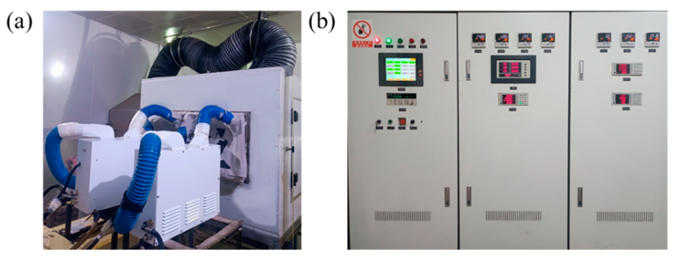
To verify the feasibility of the method proposed in this paper, an experiment on data acquisition from the sensor network of an environmental control system in a workshop is designed, and the experimental platform is shown in Figure 3. In the workshop environmental control system, the air conditioning system is not only regarded as the most critical component but also considered the most prone to failure. Therefore, the experiment in this study is primarily conducted on the sensor network of the air conditioning system within the workshop environmental control system. The experimental platform for the air conditioning system is primarily composed of the condenser, evaporator, compressor, expansion valve, experimental cabinet, and control cabinet. All experiments are carried out under cooling conditions in a standard enthalpy difference laboratory.
In the experimental platform, nine types of sensors are deployed, with details provided in Table 1. Time series data from these nine sensors are continuously collected during normal unit operation. Common summer operating conditions are simulated by adjusting the indoor and outdoor dry-bulb temperatures, with the indoor temperature regulated within a range of 23–28 °C and the outdoor temperature regulated within a range of 28–38 °C. The experimental data are collected at a frequency of 5 s. After unstable data during startup and abnormal data are removed, a total of 17,830 samples are obtained.
Due to the involvement of equipment security, trade secrets, and other factors in obtaining industrial data specific to this application scenario and containing real faults, this study followed the common practice of preliminary research in related fields and used manual fault injection to preliminarily verify the feasibility of the method [18,19]. Among these, 15,330 samples are allocated to the training set for model training, 1500 samples are used as the test set for determining fault thresholds, and 1000 samples are designated as the validation set for conducting fault diagnosis experiments.
Since the simultaneous failure of multiple sensors in the environmental control system is considered highly improbable, this study is focused exclusively on scenarios where no more than one sensor fails at the same time. Primary emphasis is placed on the diagnosis of sensor bias faults. During the operation of the environmental control system, substantial amounts of sensor fault data are difficult to obtain. Therefore, in the validation set, we introduce biases of varying magnitudes to simulate sensor fault signals caused by bias. The minimum fault level is set at 0.5% of the mean measured value of each sensor. Faults are injected at levels corresponding to 0.5%, 1%, 1.5%, and 2% of the mean measured values of respective sensors, with all fault values rounded to two decimal places. The fault injection details for sensors T1 to T9 are presented in Table 2.

4.2. Evaluation Indicators

The Root Mean Square Error (RMSE) and Mean Absolute Error (MAE) are employed to evaluate the performance of the Informer model, as shown in Equations (17) and (18). RMSE is utilized to indicate the dispersion degree of the samples, while MAE is used to assess the discrepancy between the predicted values and the actual values.
R M S E = 1 N i = 1 N z i y i 2
M A E = 1 N i = 1 N z i y i
where N is the sample quantity, z i is the predicted value, and y i is the true value.
To quantitatively evaluate sensor fault diagnosis performance, the Fault Detection Rate (FDR) is introduced to evaluate the detection status of sensor fault samples, as shown in Equation (19). The False Alarm Rate (FAR) is introduced to evaluate the scenario where normal sensor samples are misdiagnosed as faulty, as shown in Equation (20).
F D R = T P T P + F N
F A R =   F P F P + T N
where FP means False Positives, TP means True Positives, FN means False Negatives, and TN means True Negatives.
To quantitatively evaluate the sensor fault data recovery performance, the Root Mean Square Error (RMSE) and the Coefficient of Determination R2 are introduced to measure the data recovery effect, as shown in Equations (17) and (21). RMSE is used to measure the distance between the reconstructed data and the true values. R2 is used to measure the similarity between two signals. A value of R2 closer to 1 indicates a higher degree of similarity between the two signals, meaning that the reconstructed sensor data well characterizes the true values.
R 2 = 1 i = 1 n y i y i ¯ 2 i = 1 n y i y ˙ 2
where y i is the true value, y i ¯ is the predicted value, and y ˙ is the average of the true values.

4.3. Analysis of Fault Diagnosis Results

4.3.1. Prediction Results Analysis

To fully exploit the correlations within the nine-dimensional sensor data from the environmental control system, the training set of nine-dimensional sensor data is input into the Informer model for training. Multivariate predictions are performed on both the test set and validation set, with prediction steps of 1, 5, 10, 20, and 50 data points conducted. The input sequence length and prediction length are maintained at a 5:1 ratio. The evaluation results of the test set predictions are presented in Table 3.
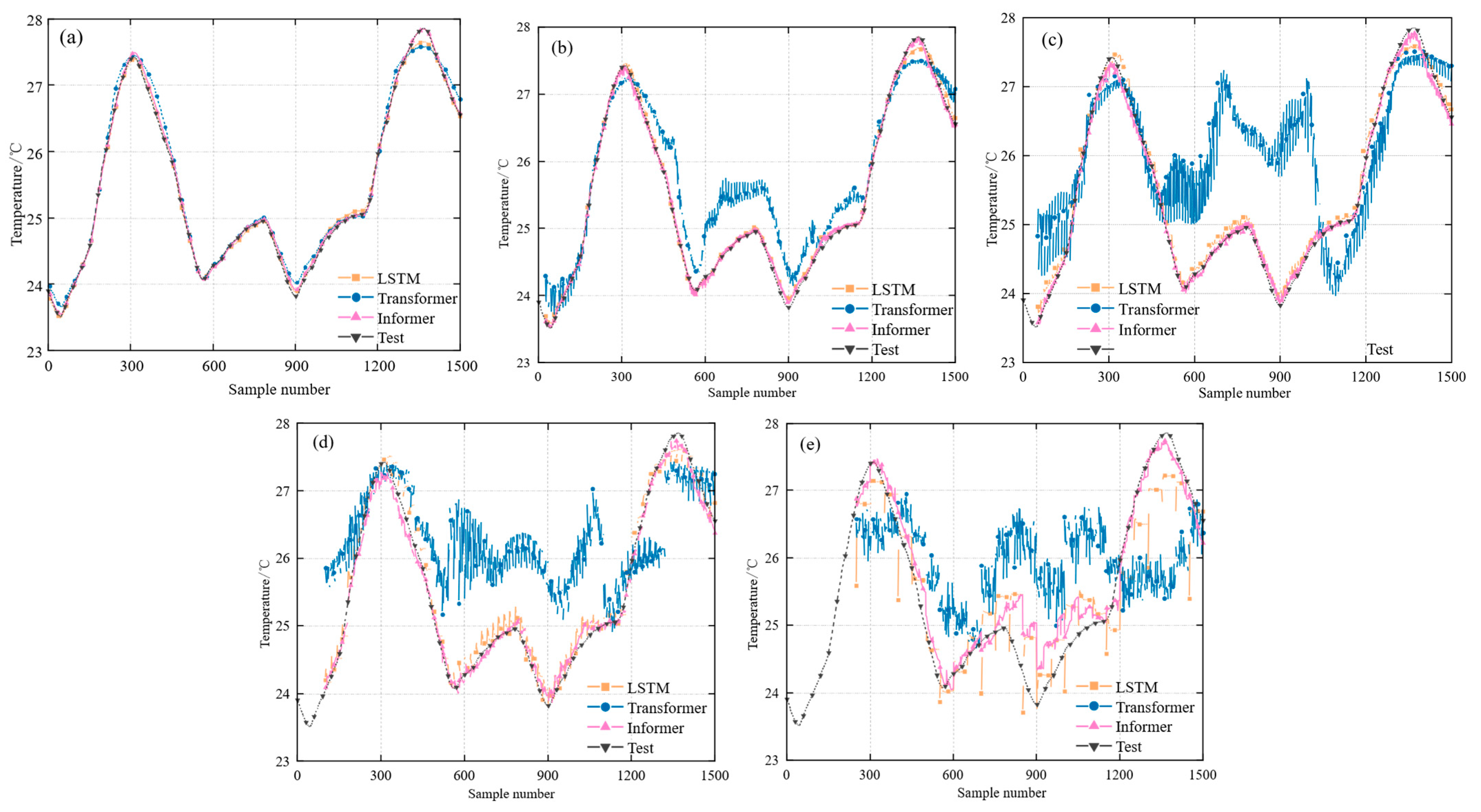
Figure 4 shows the prediction results of the LSTM, Transformer, and Informer models for sensor T1 under different prediction steps. The Informer model is observed to achieve optimal performance across all prediction steps (1, 5, 10, 20, and 50). As the prediction step is increased, the performance of all three models is found to degrade, though the Informer’s effectiveness is noted to decline more gradually. This observation demonstrates the Informer’s superior stability and robustness when handling long-term sequence predictions. Under all tested prediction steps (1, 5, 10, 20, and 50), the average RMSE and MAE values of the Informer model are lower than those of the comparative models. Specifically, the average RMSE and MAE of the Informer are reduced by 38.34% and 41.46%, respectively, when compared with those of the LSTM model.
As can be observed from Table 3, a declining trend in prediction performance is demonstrated as the prediction step length increases. Specifically, both RMSE and MAE values are shown to increase with longer step lengths. When the prediction step is set to 1, the model’s predictive performance is observed to be optimal. At this step length, the lowest RMSE and MAE values across all sensors are recorded, indicating that highly accurate single-step predictions can be achieved by the model. At step lengths of 5 and 10, respectively, although prediction errors are found to increase compared to step 1, they still remain at relatively low levels, which demonstrates the model’s maintained effectiveness in medium-term predictions. When step lengths of 20 and 50 are implemented, prediction errors are significantly increased, indicating reduced accuracy in long-term predictions. This trend is consistently observed across all sensors, suggesting that long-term prediction poses substantial challenges to the model, where error accumulation effects become significantly pronounced. The Informer model is shown to perform optimally in single-step predictions (step = 1), maintain satisfactory effectiveness in medium-term predictions (steps = 5 and 10), and exhibit noticeably increased prediction errors in long-term predictions (steps = 20 and 50).

4.3.2. Analysis of Fault Thresholds and Fault Diagnosis Results

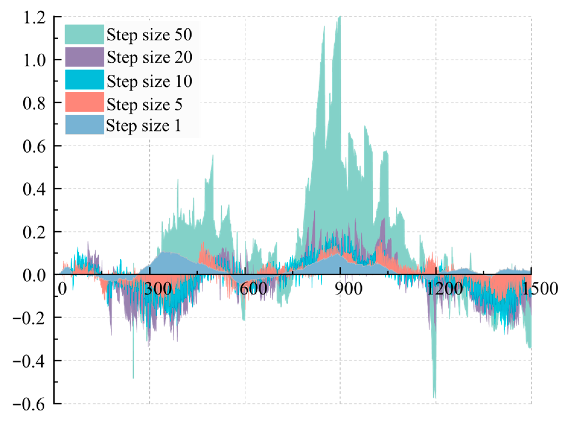
After the predicted sequence is obtained through the Informer model, the residual between the predicted value and the actual value is compared with the fault threshold to achieve fault diagnosis. Based on the threshold determination method described in Section 3.3, Table 4 shows the fault thresholds for the sensors when the prediction steps are set to 1, 5, and 10, respectively. When the calculated fault threshold exceeds 0.5% of the mean measured value of the sensor, 0.5% of the mean measured value is selected as the fault threshold. To achieve higher fault diagnosis accuracy, the fault threshold corresponding to a prediction step of 1 is chosen for subsequent fault diagnosis experiments. The residuals of the test set for sensor T1 under prediction steps of 1, 5, 10, 20, and 50 are presented in Figure 5.
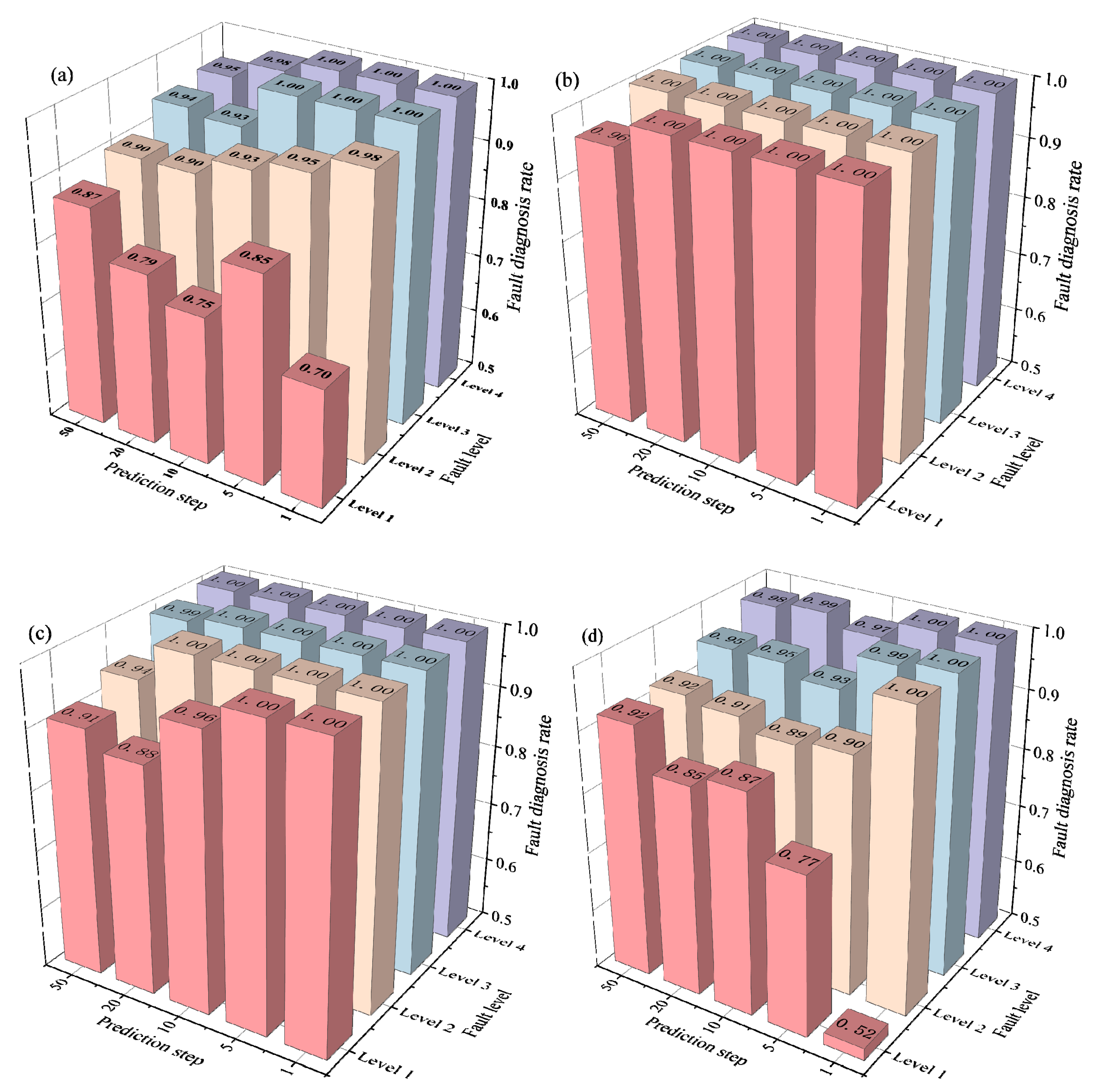
By using the selected fault threshold, fault diagnosis experiments are conducted on the validation set. As shown in Figure 6, the fault diagnosis results for four sensors (T1, T4, T5, and T9) are presented. The proposed fault diagnosis method achieves satisfactory performance across different fault levels. As the fault level increases, the manifestation of faults becomes more distinct, and better fault diagnosis results are obtained. When the prediction step is set to 10, the average fault diagnosis rates for fault levels 1, 2, 3, and 4 are 85.69%, 95.17%, 98.71%, and 99.58%, respectively. The diagnostic performance is observed to improve consistently with increasing fault severity. This indicates that the proposed method not only can be effectively used to detect minor faults but also is capable of providing accurate diagnostic results under more severe fault conditions.
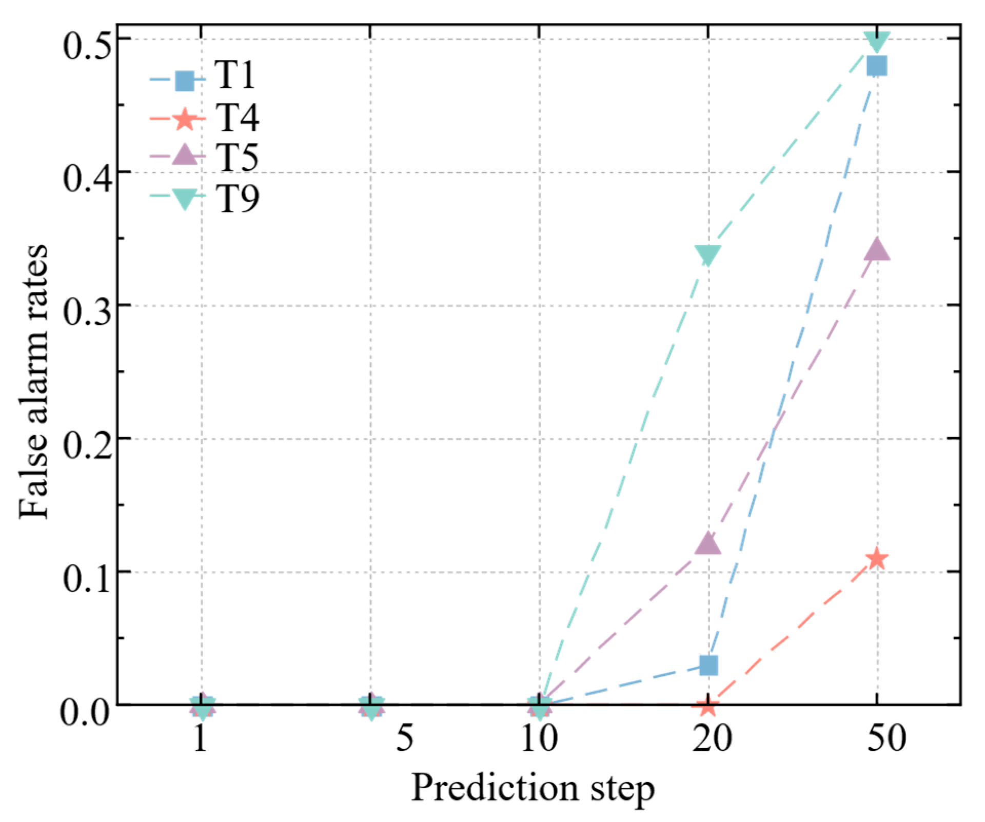
Since the false alarm rates of sensors during fault-free phases are identical across different fault levels, Figure 7 specifically demonstrates the false alarm rates for sensors T1, T4, T5, and T9 under varying prediction steps. As the prediction step length is increased, the sensor fault diagnosis rate exhibits fluctuations but generally shows a declining trend, while the false alarm rate manifests an increasing trend. Specifically, when prediction steps are set to 1, 5, 10, 20, and 50, respectively, the average fault diagnosis rates for T1–T9 are 94.40%, 95.28%, 94.79%, 92.52%, and 93.35%. The corresponding false alarm rates are measured at 0.00%, 0.56%, 1.78%, 20.33%, and 47.22%. When the prediction step is maintained at 10, relatively high fault diagnosis rates coupled with relatively low false alarm rates are achieved, indicating that the model possesses certain reliability and reference value for predicting sensor status within the next 50 s.

4.4. Fault Recovery Result Analysis

The recovery of sensor fault data is an effective method to enhance system reliability and stability, while also ensuring short-term normal operation. The sensor data recovery process is accomplished by first accurately identifying the initial fault point in the sensor data, then overwriting the faulty data with predicted values from the forecasting model, thereby achieving data recovery starting from that point. Figure 8 displays the fault location identification results for Sensor T5 under Level 2 conditions with prediction steps of 1, 5, and 10. In the validation set, where faults are introduced starting from the 100th data point, all sensor data are successfully maintained within the fault threshold range after recovery processing. Simultaneously, Figure 9 presents the data recovery results for Sensor T5 under prediction steps of 1, 5, and 10. The reconstructed data closely approximate the actual values, with all reconstructed data points remaining within the fault threshold range. This demonstrates that the reconstructed data can effectively recover faulty sensor data.
As can be observed from Table 5, the RMSE values exhibit an increasing trend while the R2 values demonstrate a decreasing trend as the prediction step length is extended. This pattern indicates that prediction errors are progressively increased and the model’s data fitting capability is correspondingly reduced. When the prediction step length is extended beyond 20, the RMSE values are significantly elevated and R2 values are markedly decreased, which can be attributed to the substantial challenges faced by the model in long-term predictions where forecasting accuracy is considerably diminished. However, when the prediction step length is maintained within 10, all predicted data are successfully contained within the fault threshold range. These predicted values can be effectively utilized to replace faulty data, thereby achieving successful recovery of sensor network faults in the workshop environmental control system.

5. Conclusions

(1)
Compared with the LSTM and Transformer models, the Informer model achieves superior performance on long time series, exhibiting the best prediction results at step lengths of 1, 5, 10, 20, and 50. This capability enables accurate state prediction within the sensor’s prediction horizon. Specifically, the experiment with a prediction step of 10 achieves both high fault diagnosis rates and low false alarm rates, confirming the method’s effectiveness in predicting sensor states for up to 50 s into the future.
(2)
For the same sensor, improved fault diagnosis performance is observed with higher fault levels. The average fault diagnosis rates for Level 1 to Level 4 are recorded as 85.69%, 95.17%, 98.71%, and 99.58%, respectively. At prediction steps of 1, 5, 10, 20, and 50, the average diagnosis rates for T1–T9 sensors are maintained at 94.40%, 95.28%, 94.79%, 92.52%, and 93.35%, demonstrating effective fault diagnosis capability across various conditions.
(3)
Through medium-to-long-term prediction, faulty data recovery is successfully achieved in this study. The reconstructed data are guaranteed to remain within the fault threshold range, enabling short-term data restoration. System operation can be maintained under sensor fault conditions through this approach. This method has been established as providing a viable medium-to-long-term prediction solution for sensor network fault diagnosis in workshop environmental control systems. Future research should be directed toward exploring methods to increase prediction step lengths while ensuring diagnostic accuracy and reliability.
(4)
Adapting this method to new applications does indeed incur a one-time initial model training cost, but its long-term operation and calibration costs are low. Therefore, we believe that this method has significant competitiveness in terms of cost-effectiveness. Its one-time upfront investment can bring long-term reliability and stability improvement to industrial systems, avoiding huge economic losses caused by sudden failures, thus having high practical application value and return rate.

Author Contributions

Writing—Original Draft, S.X.; Writing—review & editing, F.Y.; Investigation, X.Z.; Validation, M.T.; Resources, C.Z. All authors have read and agreed to the published version of the manuscript.

Funding

This study was funded by the Natural Science Foundation of Hubei Province Grants No. 2023AFB400, and the Hubei University of Technology Research Fund under Grants BSQD2020009.

Data Availability Statement

Data are contained within the article.

Conflicts of Interest

The authors declare no conflicts of interest.

References

  1. Negi, V.P.S.; Ranganayakulu, C. Energy-efficient three-wheel bleedless electrical environmental control system for a passenger aircraft. J. Appl. Therm. Sci. Eng. Appl. 2025, 17, 021009. [Google Scholar] [CrossRef]
  2. Jennions, I.; Ali, F.; Miguez, M.E.; Escobar, I.C. Simulation of an aircraft environmental control system. J. Appl. Therm. Eng. 2020, 172, 114925. [Google Scholar] [CrossRef]
  3. Verma, P.; Kumar, V.; Daim, T.; Sharma, N.K. Design thinking framework toward management control system in environmental dynamism: An innovation perspective. J. IEEE Trans. Eng. Manag. 2024, 71, 4955–4970. [Google Scholar] [CrossRef]
  4. Petera, P.; Wagner, J.; Paksiova, R. The Influence of environmental strategy, environmental reporting and environmental management control system on environmental and economic performance. J. Energ. 2021, 14, 4637. [Google Scholar] [CrossRef]
  5. Cozza, A. Low frequency model-based identification of soft impedance faults in cables. J. IEEE Trans. Instrum. Meas. 2019, 68, 3524–3535. [Google Scholar] [CrossRef]
  6. Ginzarly, R.; Moubayed, N.; Hoblos, G.; Kanj, H.; Alakkoumi, M.; Mawas, A. Assessing HMM and SVM for condition-based monitoring and fault detection in HEV electrical machines. J. Energ. 2025, 18, 3513. [Google Scholar] [CrossRef]
  7. Yan, K.; Zhong, C.W.; Ji, Z.W.; Huang, J. Semi-supervised learning for early detection and diagnosis of various air handling unit faults. J. Energy Build. 2018, 181, 75–83. [Google Scholar] [CrossRef]
  8. Orellana, C.; Ortiz, L.; Aguila, A.; Garcia, M.; Ruiz, M. Hybrid algorithm for fault detection in three-phase motors using principal component analysis. J. E-Prime—Adv. Electr. Eng. Electron. Energy 2025, 11, 100916. [Google Scholar] [CrossRef]
  9. Mao, Q.J.; Fang, X.; Hu, Y.P.; Li, G. Chiller sensor fault detection based on empirical mode decomposition threshold denoising and principal component analysis. J. Appl. Therm. Eng. 2018, 144, 21–30. [Google Scholar] [CrossRef]
  10. Zhong, X.P.; Zhang, L.; Ban, H. Deep reinforcement learning for class imbalance fault diagnosis of equipment in nuclear power plants. J. Ann. Nucl. Energy 2023, 184, 109685. [Google Scholar] [CrossRef]
  11. Gins, G.; Kerkhof, D.V.P.; Vanlaer, J.; Van Impe, J.F. Improving classification-based diagnosis of batch processes through data selection and appropriate pretreatment. J. Process Control 2015, 26, 90–101. [Google Scholar] [CrossRef]
  12. Wang, X.; Shen, C.Q.; Xia, M.; Wang, D.; Zhu, J.; Zhu, Z. Multi-scale deep intra-class transfer learning for bearing fault diagnosis. J. Reliab. Eng. Syst. Saf. 2020, 202, 107050. [Google Scholar] [CrossRef]
  13. Li, G.N.; Xiong, C.L.; Gao, J.J.; Zhu, H.; Wang, C.; Xiao, J. Fault detection, diagnosis and calibration of heating, ventilation and air conditioning sensors by combining principal component analysis and improved bayesian inference. J. Build. Eng. 2024, 82, 108230. [Google Scholar] [CrossRef]
  14. Zhou, H.Y.; Zhang, S.H.; Peng, J.Q.; Zhang, S.; Li, J.; Xiong, H.; Zhang, W. Informer: Beyond efficient transformer for long sequence time-series forecasting. Proc. AAAI Conf. Artif. Intell. 2021, 35, 11106–11115. [Google Scholar] [CrossRef]
  15. Li, F.Y.; Wan, Z.B.; Koch, T.; Zan, G.; Li, M.; Zheng, Z.; Liang, B. Improving the accuracy of multi-step prediction of building energy consumption based on EEMD-PSO-Informer and long-time series. J. Comput. Electr. Eng. 2023, 110, 108845. [Google Scholar] [CrossRef]
  16. Guo, L.; Li, R.Z.; Jiang, B. A data-driven long time-series electrical line trip fault prediction method using an improved stacked-informer network. J. Sens. 2021, 21, 4466. [Google Scholar] [CrossRef] [PubMed]
  17. Klimek, J.; Jakub, K.; Kraśkiewicz, W.; Topolewski, M. Long-term series forecasting with query selector-efficient model of sparse attention. J. Softw. Impacts 2022, 11, 100187. [Google Scholar] [CrossRef]
  18. Xu, S.Q.; Yu, H.Y.; Wang, H.; Chai, H.; Ma, M.; Chen, H.; Zheng, W.X. Simultaneous diagnosis of open-switch and current sensor faults of inverters in IM drives through reduced-order interval observer. J. IEEE Trans. Ind. Electron. 2025, 72, 6485–6496. [Google Scholar] [CrossRef]
  19. Shaheen, K.; Chawla, A.; Rossi, P.S. Trust-Enhanced Distributed Kalman Filtering for Sensor Fault Diagnosis in Sensor Networks. J. IEEE Trans. Signal Inf. Process. Over Netw. 2025, 11, 1178–1187. [Google Scholar] [CrossRef]
Figure 1. Principle of state prediction.
Machines 13 00975 g001
Figure 2. Initial fault data identification and recovery process.
Machines 13 00975 g002
Figure 3. Environmental control system experimental platform: (a) experimental platform; (b) control system.
Machines 13 00975 g003
Figure 4. Prediction results of the LSTM, Transformer, and Informer models for sensor T1 under different prediction steps: (a) 1; (b) 5; (c) 10; (d) 20; (e) 50.
Machines 13 00975 g004
Figure 5. Residuals of Sensor T1 under different prediction steps.
Machines 13 00975 g005
Figure 6. Sensor fault diagnosis rate for four sensors (a) T1; (b) T4; (c) T5; (d) T9.
Machines 13 00975 g006
Figure 7. Distribution of False Alarm Rates for Sensor Bias Faults.
Machines 13 00975 g007
Figure 8. Fault location identification results for Sensor T5 under Level 2 conditions with different prediction steps: (a) 1; (b) 5; (c) 10.
Machines 13 00975 g008
Figure 9. Data recovery results for Sensor T5 under different prediction steps: (a) 1; (b) 5; (c) 10.
Machines 13 00975 g009
Table 1. Description of sensors in the environmental control system.
NumberTest PointSymbolUnit
1Indoor side air inlet dry-bulb temperatureT1°C
2Outdoor side air inlet dry-bulb temperatureT2°C
3Compressor inlet temperatureT3°C
4Compressor outlet temperatureT4°C
5Condenser inlet temperatureT5°C
6Condenser outlet temperatureT6°C
7Evaporator inlet temperatureT7°C
8Evaporator outlet temperatureT8°C
9Expansion valve outlet temperatureT9°C
Table 2. Simulated conditions of sensors with varying levels of bias faults.
SensorsLevel 1 (0.5%)Level 2 (1%)Level 3 (1.5%)Level 4 (2%)
T1−0.13, 0.13−0.25, 0.25−0.38, 0.38−0.51, 0.51
T2−0.17, 0.17−0.34, 0.34−0.50, 0.50−0.67, 0.67
T3−0.09, 0.09−0.17, 0.17−0.26, 0.26−0.34, 0.34
T4−0.50, 0.50−1.00, 1.00−1.50, 1.50−2.00, 2.00
T5−0.39, 0.39−0.78, 0.78−1.17, 1.17−1.56, 1.56
T6−0.23, 0.23−0.46, 0.46−0.69, 0.69−0.93, 0.93
T7−0.20, 0.20−0.40, 0.40−0.60, 0.60−0.80, 0.80
T8−0.04, 0.04−0.08, 0.08−0.11, 0.11−0.15, 0.15
T9−0.06, 0.06−0.13, 0.13−0.19, 0.19−0.25, 0.25
Table 3. Evaluation Metrics of the Informer Model for Different Forecasting Sequence Lengths.
Sensor15102050
RMSEMAERMSEMAERMSEMAERMSEMAERMSEMAE
T10.04170.03160.05360.04190.08080.06360.12590.10540.35660.2674
T20.05240.03830.12060.09990.12520.09700.11680.09110.29100.2101
T30.02480.02180.04310.03490.04660.03870.06800.05680.11950.1017
T40.04230.03170.05490.04390.07420.05790.11110.08400.25040.1923
T50.03920.02990.09090.06820.13170.10110.20750.16080.50600.4106
T60.06630.05330.08920.07270.12100.09290.18400.13800.45860.3204
T70.04400.03500.09610.07340.12850.09640.19940.15150.52600.3852
T80.02750.02220.03660.02850.04940.03860.06800.05110.20800.1627
T90.02520.01860.05960.04700.09910.07910.16710.12300.38520.2829
Table 4. Sensor fault threshold under different prediction steps.
Sensor1510
T1(−0.11, 0.11)(−0.18, 0.18)(−0.28, 0.28)
T2(−0.15, 0.15)(−0.37, 0.37)(−0.47, 0.47)
T3(−0.06, 0.06)(−0.13, 0.13)(−0.14, 0.14)
T4(−0.13, 0.13)(−0.17, 0.17)(−0.30, 0.30)
T5(−0.17, 0.17)(−0.38, 0.38)(−0.44, 0.44)
T6(−0.18, 0.18)(−0.33, 0.33)(−0.44, 0.44)
T7(−0.12, 0.12)(−0.34, 0.34)(−0.46, 0.46)
T8(−0.04, 0.04)(−0.12, 0.12)(−0.16, 0.16)
T9(−0.06, 0.06)(−0.15, 0.15)(−0.24, 0.24)
Table 5. Evaluation results of faulty data recovery by fault-compensated soft sensors.
Sensor15102050
RMSER2RMSER2RMSER2RMSER2RMSER2
T10.05650.99820.06780.99740.11110.99300.21970.9730 0.55950.8250
T20.06230.99940.15640.99650.15510.99650.17130.99580.38190.9793
T30.01990.99940.04840.99650.05100.99610.09240.98740.11030.9820
T40.03860.99920.06710.99780.06980.99760.09620.9956 0.21030.9790
T50.05000.99950.10790.99780.14280.99620.22610.99060.56330.9416
T60.07420.99930.12160.99820.17760.99620.26120.99180.66550.9470
T70.06510.99920.13920.99670.18230.99430.27760.98690.72800.9103
T80.02610.99870.04770.99580.06800.99150.11360.97640.30770.8274
T90.02310.99960.07150.99660.11920.99050.2183 0.96840.49050.8408
Disclaimer/Publisher’s Note: The statements, opinions and data contained in all publications are solely those of the individual author(s) and contributor(s) and not of MDPI and/or the editor(s). MDPI and/or the editor(s) disclaim responsibility for any injury to people or property resulting from any ideas, methods, instructions or products referred to in the content.