Adaptive PI Control Using Recursive Least Squares for Centrifugal Pump Pipeline Systems

Abstract

Pipeline transportation of petroleum products remains one of the safest and most efficient methods of bulk energy delivery, yet overpressure events continue to pose serious operational and regulatory challenges. Traditional fixed-gain PI controllers, commonly used with centrifugal pump drives, cannot adapt to varying product densities or transient disturbances such as valve closures that generate water hammer. This paper proposes a self-tuning adaptive controller based on Recursive Least Squares (RLS) parameter estimation to improve safety and efficiency in pipeline pump operations. A nonlinear simulation model of a centrifugal pump driven by an induction motor is developed, incorporating pipeline friction losses via the Darcy–Weisbach relation and pressure transients induced by rapid valve closures. The RLS algorithm continuously estimates effective loop dynamics, enabling online adjustment of proportional and integral gains under changing fluid and operating conditions. Simulation results demonstrate that the proposed RLS-based adaptive controller maintains discharge pressure within ±2% of the target setpoint under density variations from 710 to 900 kg/m³ and during severe transient events. Compared to a fixed-gain PI controller, the adaptive strategy reduced pressure overshoot by approximately 31.9% and settling time by 6%. Model validation using SCADA field data yielded an $R^2$ = 0.957, RMSE = 3.95 m³/h, and normalized NRMSE of 12.6% (by range), confirming strong agreement with measured system behavior. The findings indicate that RLS-based self-tuning provides a practical enhancement to existing pipeline control architectures, offering both improved robustness to abnormal transients and greater efficiency during steady-state operation. This work establishes a foundation for higher-level supervisory and game-theoretic coordination strategies to be explored in subsequent studies.

1. Introduction

The transition toward alternative energy sources is accelerating, yet petroleum-based fuels and products remain essential in the foreseeable future. Transportation, power generation, and plastics manufacturing still rely heavily on pipelines as the safest and most cost-effective method of moving large volumes of hydrocarbons [1]. However, aging infrastructure, construction-based spacing constraints, and varying operational scenarios can introduce vulnerabilities—especially in pressure regulation along the pipeline.

One such tragic event that highlighted the importance of proper pressure control occurred in Bellingham, Washington, in 1999, where a series of system failures, including a pressure surge, led to a pipeline rupture, causing three deaths, massive environmental damage, and a fireball reaching 30 stories high [2]. Investigations revealed that inadequate real-time pressure response and control mechanisms contributed to the pipeline’s inability to stabilize following valve operations and transient conditions. This event highlights an urgent need for intelligent and adaptive pressure control strategies that can respond in real time to changing conditions.

Modern pipelines often transport different product batches with varying fluid densities, significantly altering pipeline dynamics. Traditional controllers are typically tuned for a single steady-state condition based on average operating scenarios. Although this fixed-gain approach offers stability under designed conditions, it becomes rigid and suboptimal when the system dynamics change due to fluid properties, valve operations, or pump degradation. This rigidity can lead to poor control, increased energy consumption, or dangerous overpressure events.

Centrifugal pump and pipeline systems inherently exhibit multi-scale fluid excitation phenomena that complicate dynamic pressure regulation and control. At the pump scale, blade-passing interactions, impeller–volute asymmetry, and internal recirculation induce high-frequency pressure pulsations and hydraulic excitations that modulate the instantaneous head–flow relationship [3,4,5]. At the pipeline scale, these local disturbances interact with lower-frequency system transients such as valve closures, pump speed changes, and pressure-wave reflections along the pipe. The combined effect produces coupled dynamics across multiple scales, resulting in nonlinear, non-stationary pressure and flow oscillations. These multi-scale interactions are particularly challenging for fixed-gain controllers, as their tuning is typically based on quasi-steady conditions and cannot adapt to transient coupling between pump excitation and pipeline resonance modes. Accurately mitigating these effects motivates the use of adaptive estimation and learning-based supervisory strategies that can respond to time-varying hydraulic conditions in real time.

Adaptive controllers, refs. [6,7,8,9], based on Recursive Least Squares (RLS), remain a cornerstone method for online parameter estimation and adaptive control due to their fast convergence, recursive structure, and computational efficiency [10,11]. In industrial process control, the challenge of adapting controllers under varying operating conditions motivates the exploration of enhanced RLS schemes that ensure both robustness and accuracy, particularly those incorporating variable forgetting factors, regularization, and bias compensation, which significantly extends the applicability of RLS to nonlinear and time-varying systems.

Adaptive control techniques based on recursive estimation have long been applied to process systems to accommodate time-varying dynamics and uncertain operating conditions. The Recursive Least Squares (RLS) algorithm, in particular, has been widely used for online parameter identification and controller tuning. Early adaptive control frameworks—such as those described by Åström [12]—focused on indirect adaptive control, where the RLS estimator identifies a plant model (typically in Auto-Regressive with eXogenous (ARX or ARMAX) form), and controller parameters are subsequently derived from that model.

More recently, several studies have explored direct adaptive control schemes, in which the RLS algorithm operates on the controller law rather than the plant model. Direct RLS adaptation, as demonstrated by Fahmy et al. [13], can stabilize stable and unstable single-input–single-output systems without explicit plant modeling. Similarly, Silveira and Brito [14] presented an RLS-based direct self-tuning PID approach that updates controller parameters in real time using measured control errors and control signals. These works established the feasibility of direct RLS adaptation but focused primarily on process control or simulation case studies unrelated to fluid transport.

Variable forgetting factor RLS algorithms have been successfully applied to vehicle state estimation, where parameter tracking must remain robust despite rapid dynamics and noise [15]. In energy systems, bias-compensated forgetting factor RLS has been shown to accurately track battery model parameters under non-stationary conditions [16]. In signal processing, filtered-x RLS algorithms have been developed for active noise control, demonstrating improved convergence in noisy environments [17]. Similarly, adaptive MIMO control architectures have employed RLS-based parameter self-tuning to handle unknown multivariable dynamics [18]. Regularization strategies for RLS have also been introduced to mitigate parameter drift and enhance robustness against noise [19], while rank-reduced update formulations have improved numerical stability and convergence speed [20].

This highlights that RLS and its modern variants remain competitive for real-time parameter tracking. Advances such as generalized forgetting factors [21], robust regularization schemes [22,23], and low-complexity update formulations [20,24] have extended the stability and applicability of RLS in noisy and time-varying environments. In parallel, however, the pipeline literature has largely adopted extended Kalman filters and machine learning approaches for leak detection and transient modeling [25,26,27], yet these methods often demand higher computational resources and complex models. The relative scarcity of RLS implementations in pipeline systems underscores a gap that this work seeks to address.

Together, these contributions illustrate that RLS is not only an established algorithm but also an evolving framework that adapts to diverse engineering domains. The successes of variable forgetting factor and regularized RLS approaches in vehicles, batteries, and active control provide direct evidence that similar adaptations can be leveraged for pipeline process control loops. Building on this foundation, the present work proposes an RLS-based loop-level adaptation framework for pipeline pump stations. The method enables continuous tuning that maintains stability and efficiency under changing hydraulic conditions by embedding recursive parameter estimation with adaptive forgetting into local control. This aligns with recent developments in adaptive estimation while addressing the unique challenges of distributed pipeline operations.

Although one might question whether the adaptation should stop once the system reaches steady-state behavior, such a strategy is shortsighted. Pipeline conditions can change over time due to factors such as temperature fluctuations, fouling, or wear of components. As these dynamics evolve, fixed gain settings may become outdated. Sudden events—like valve closures or product switching—demand that controllers stay agile and responsive. If gains are set based on limited operating data, there is a risk of parameter estimation bias. Maintaining an adaptive system helps ensure that gains are properly tuned across a wider range of conditions. Robustness to model mismatch and unmodeled nonlinearities is improved with continued adaptation. Persistent excitation, maintained through slight continuous variation, keeps the RLS algorithm accurate and responsive.

In the context of pipeline and pump station systems, most existing adaptive control studies continue to rely on indirect RLS estimation of hydraulic parameters or flow–pressure relationships [28,29]. The resulting plant models are then used to retune pump speed or valve position controllers. While effective, these methods introduce additional computational overhead and depend on accurate model identification, which may be challenging under transient or multiphase flow conditions.

This work applies a direct RLS-based self-tuning controller to centrifugal pump or pipeline systems by embedding the ARX-style recursive estimator directly within the controller law. This work, therefore, introduces a novel approach wherein the velocity-form controller is parameterized as a linear regression, allowing the RLS algorithm to estimate and adapt the proportional and integral gains, $\{K_p,K_i\}$, directly from measured control error and actuation signals. This configuration reduces dependence on external model identification, simplifies implementation, and provides a foundation for higher-level reinforcement learning and game-theoretic coordination developed in subsequent studies.

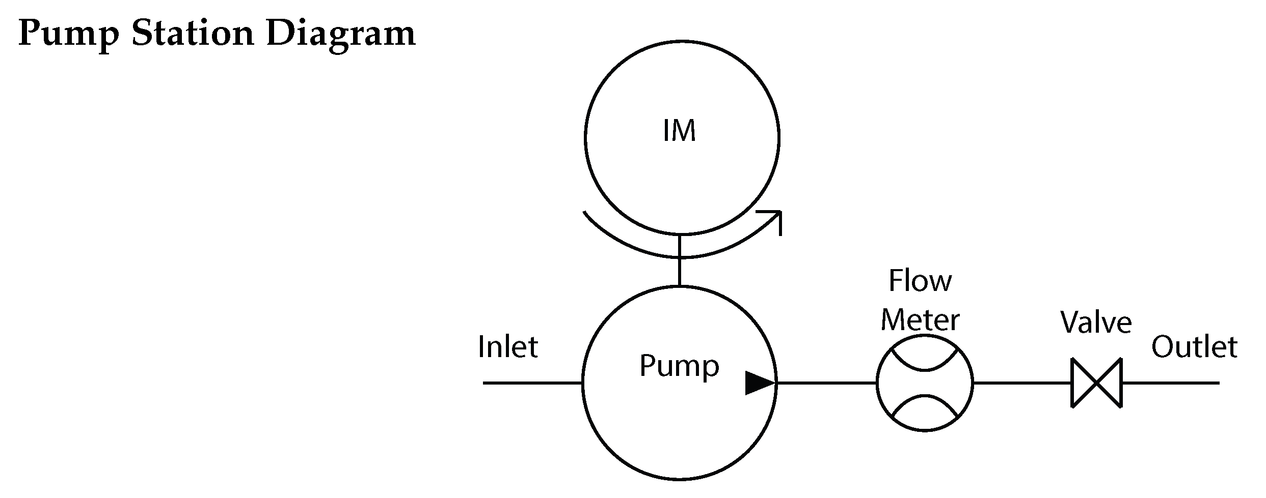
There is research on the subject of adaptive control at the programmable logic controller (PLC) level, refs. [9,30,31], but the theory has not yet been applied in real-world pipeline control. The algorithm presented in this paper can be applied to a real-time single-pump and pipeline loop at the PLC level. The system can dynamically adjust its response to changing product density and pipeline dynamics using a velocity form controller embedded with RLS gain estimation with a variable forgetting factor. The approach is validated using nonlinear system models of an induction motor–centrifugal pump–pipeline system, emphasizing pressure regulation and robustness to overpressure transients (Figure 1).

This foundational step lays the groundwork for later extensions to multi-loop Q-Table coordination and inter-station negotiation, forming a layered and scalable adaptive control strategy for future pipeline networks.

The whole control framework is tested in MATLAB R2023b using a nonlinear simulation model of an induction motor-driven centrifugal pump pipeline system. The model captures energy use, head pressure, and dynamic responses to pipeline transients, including overpressure transients (Figure 1). The simulation model was validated against historical SCADA data from fixed-gain control operation, demonstrating strong agreement with field measurements and confirming its reliability for adaptive control analysis. The layered design enables each station to adapt locally, coordinate internally, and negotiate globally, forming a robust and scalable architecture for modern pipeline systems.

2. Model Description

The simulation model developed in this study consists of four main components: an induction motor, a centrifugal pump, a fluid-filled pipeline, and a velocity-form controller enhanced with a variable forgetting factor, Recursive Least Squares (RLS) for self-tuning. The model effectively captures the essential dynamics of each component, demonstrating the performance and robustness of the adaptive control strategy.

2.1. Induction Motor and Pump

The induction motor is modeled as a dynamic torque source controlled by a variable frequency drive (VFD) [9], which regulates the motor speed in response to the output of the controller. A simplified dynamic model is used to represent the inertia of the rotor and the speed response, ref. [32], given by:

$$J{\displaystyle \frac{d\omega }{dt}}=T_m-T_l-B\omega$$

(1)

where J is the combined inertia of the motor and the pump ($\mathrm{kg}·{\mathrm{m}}^2$), $\omega$ is the angular speed of the motor (rad/s), $T_m$ is the torque of the motor ($\mathrm{N}·\mathrm{m}$), $T_l$ is the load torque imposed by the pressure of the pump and pipeline ($\mathrm{N}·\mathrm{m}$), and B represents the losses of rotational friction. The motor torque is assumed to respond instantaneously to VFD commands for simulation purposes.

The centrifugal pump is modeled using a nonlinear pressure–flow relationship consistent with standard pump curves [33,34,35], expressed as:

$$H(\omega ,Q)=a_{h0}{\omega }^2-a_{h1}\omega Q-a_{h2}{Q}^2,$$

(2)

$$Q=k·\omega$$

(3)

where H is the pump head (m), which is a function of both the angular speed $\omega$ and Q, and contains parameters $a_{h0}$, $a_{h1}$, and $a_{h2}$ taken from the pump curve and determined using least squares. Q is the flow rate (m³/s), k is a constant relating speed to flow, and $\omega$ is the pump speed. Variations in fluid density are introduced to simulate batch effects, which influence the pump head and pipeline resistance.

2.2. Pipeline and Valve Dynamics

The pipeline model considers both steady-state flow resistance and dynamic pressure behavior. Fluid flow through a pipeline experiences head loss due to friction, which can be modeled using the Darcy–Weisbach equation [33]

$$h_f=f·{\displaystyle \frac{L}{D}}·{\displaystyle \frac{v^2}{2g}}$$

(4)

where $h_f$ is the frictional head loss (m), f is the Darcy friction factor (dimensionless), L is the pipe length (m), D is the pipe diameter (m), v is the fluid velocity (m/s), and g is the gravitational acceleration ($9.81{\mathrm{m}/\mathrm{s}}^2$).

The pressure drop associated with $h_f$ contributes to the total dynamic head that the pump must overcome. The Darcy friction factor f can be obtained from the Moody chart or approximated using empirical formulas such as the Colebrook-White equation for turbulent flow.

Transient pressure surges occur when flow is rapidly changed—such as during a valve closure—creating a pressure wave that travels back through the pipeline. This phenomenon, known as water hammer, is modeled using the Joukowsky equation [36]

$$\Delta P=\rho a\Delta v$$

(5)

where $\Delta P$ is the increase in pressure due to the transient (Pa), $\rho$ is the density of the fluid (kg/m³), a is the speed of the pressure wave (m/s), and $\Delta v$ is the change in fluid velocity (m/s).

The pressure wave speed a [33] depends on the elasticity of both the fluid and the pipe wall and is given by

$$a=\sqrt{{\displaystyle \frac{K}{\rho \left(1+\frac{KD}{Ee}\right)}}}$$

(6)

where K is the bulk modulus of the fluid (Pa), E is the Young’s modulus of the pipe material (Pa), and e is the pipe wall thickness (m). In this case, $E\gg K$ so the term ${\displaystyle \frac{KD}{Ee}}\ll 1$ becomes negligible, so the equation for a simplifies to

$$a=\sqrt{{\displaystyle \frac{K}{\rho }}}$$

(7)

These dynamics are critical to model accurately, as a sudden valve closure can result in a large positive pressure surge. If not mitigated, this surge can exceed the Maximum Allowable Operating Pressure (MAOP) and cause damage or rupture. The controller must respond proactively to such events, making adaptive tuning crucial to mitigating transient risks.

For simulation purposes, a pressure wave is initiated in the model by closing the valve at the downstream boundary. The assumption here is that the valve closing timing is greater than or equal to the critical closing time ($t_c$),

$$\begin{array}{c}\hfill t_c={\displaystyle \frac{2L}{a}},\end{array}$$

(8)

so the peak pressure increase, $\Delta P$, is scalable. The wave propagation and reflection behavior depend on the pipeline geometry, boundary conditions, and fluid compressibility. The resulting pressure transients are superimposed onto the steady-state pressures and used to test the responsiveness of the adaptive controller.

2.3. Velocity-Form Controller

A discrete-time controller is implemented in velocity form to allow gain updates without introducing offset. The controller is given by [37,38,39]:

$$\Delta u\left(k\right)=K_p[e\left(k\right)-e(k-1)]+K_{i}e\left(k\right)$$

(9)

$$u\left(k\right)=u(k-1)+\Delta u\left(k\right)$$

(10)

where $e\left(k\right)$ is the control error (difference between pressure setpoint and measured pressure), $u\left(k\right)$ is the controller output (used to command the VFD), and $K_p$, $K_i$ are the proportional and integral gains, respectively. The RLS algorithm updates these gains in real time based on system identification. Since pressure is measured by a pressure transmitter, a random noise signal will be injected into the pressure value sent to the controller.

2.4. Recursive Least Squares Estimator

To adapt to changing pipeline conditions, the controller includes an online RLS estimator, refs. [6,38,39], that fits a linear model to the input–output relationship:

$$y\left(k\right)={\theta }_{1}u(k-1)+{\theta }_{2}y(k-1)+\epsilon \left(k\right)$$

(11)

The RLS algorithm recursively estimates the parameter vector $\theta ={[{\theta }_1,{\theta }_2]}^{\top }$ using the update equations:

$$\begin{array}{cc}\hfill K\left(k\right)& ={\displaystyle \frac{P(k-1)\varphi \left(k\right)}{\lambda +{\varphi }^{\top }\left(k\right)P(k-1)\varphi \left(k\right)}}\hfill \end{array}$$

(12)

$$\begin{array}{cc}\hfill \widehat{\theta }\left(k\right)& =\widehat{\theta }(k-1)+K\left(k\right)[y\left(k\right)-{\varphi }^{\top }\left(k\right)\widehat{\theta }(k-1)]\hfill \end{array}$$

(13)

$$\begin{array}{cc}\hfill P\left(k\right)& ={\displaystyle \frac{1}{\lambda }}[P(k-1)-K\left(k\right){\varphi }^{\top }\left(k\right)P(k-1)]\hfill \end{array}$$

(14)

where $\varphi \left(k\right)={[u(k-1),y(k-1)]}^{\top }$ is the regressor vector, P is the covariance matrix, $\lambda$ is the forgetting factor ($0.95<\lambda <1.0$), and $\widehat{\theta }$ is the estimated parameter vector. The controller gains $K_p$ and $K_i$ are then computed based on these estimates, using a predefined mapping that maintains stability and damping margins.

2.5. Simulation Parameters

The simulation is performed in MATLAB 2023b over a period sufficient to observe pressure transients and the controller’s adaptation behavior. The fluid density is varied mid-simulation to simulate product switching, and the valve is closed at specific time intervals to trigger overpressure conditions. The RLS controller is compared to a fixed-gain PI controller to assess its ability to maintain pressure control while reducing overshoot and energy input. The assumptions made in this research are: Fluid properties: Incompressible flow with constant density and viscosity over the control horizon, except during the product change, when the two densities are considered to calculate the line fill and flow rates. Pump behavior: Performance curves remain fixed within each control cycle; changes arise only from commanded speed adjustments. Transient modeling: Pressure waves are modeled using the simplified Joukowsky relation, where higher-order reflections and minor losses are neglected. Measurements: Pressure is the only “sensor” available to the controller, and the measurement noise is treated as zero-mean Gaussian.

2.6. Model Validation

A validation study was performed using historical SCADA data from the operating pipeline station to ensure that the proposed control-oriented pump and pipeline model accurately represents the physical system dynamics. The dataset includes measured pump discharge pressure responses during flow setpoint changes. The validation data was provided by a pipeline operator for research purposes only and is not publicly available. The validation process compared the simulated closed-loop response of the model under fixed gain control to field measurements obtained during normal operating events, specifically flow setpoint changes executed under a constant-gain controller.

In the validation tests, the same controller gains used in the field were applied within the simulation environment. The pump block was parameterized using the manufacturer’s head–flow–speed performance curve, while the pipeline section was modeled with friction and compressibility coefficients tuned within physically reasonable limits. The SCADA data were preprocessed to align sampling rates and time stamps with the simulation time base, and the same setpoint sequences were replayed in the model.

Quantitative performance was assessed using standard metrics, including the root mean squared error (RMSE), normalized RMSE (NRMSE) by range, and the coefficient of determination ($R^2$):

$$\mathrm{NRMSE}={\displaystyle \frac{\sqrt{\frac{1}{N}{\sum }_{i=1}^N{(y_i-{\widehat{y}}_i)}^2}}{y_{max}-y_{min}}}\times 100\%,R^2=1-{\displaystyle \frac{\sum {(y_i-{\widehat{y}}_i)}^2}{\sum {(y_i-\overline{y})}^2}}$$

where $y_i$ and ${\widehat{y}}_i$ denote the measured and simulated flow rate, respectively.

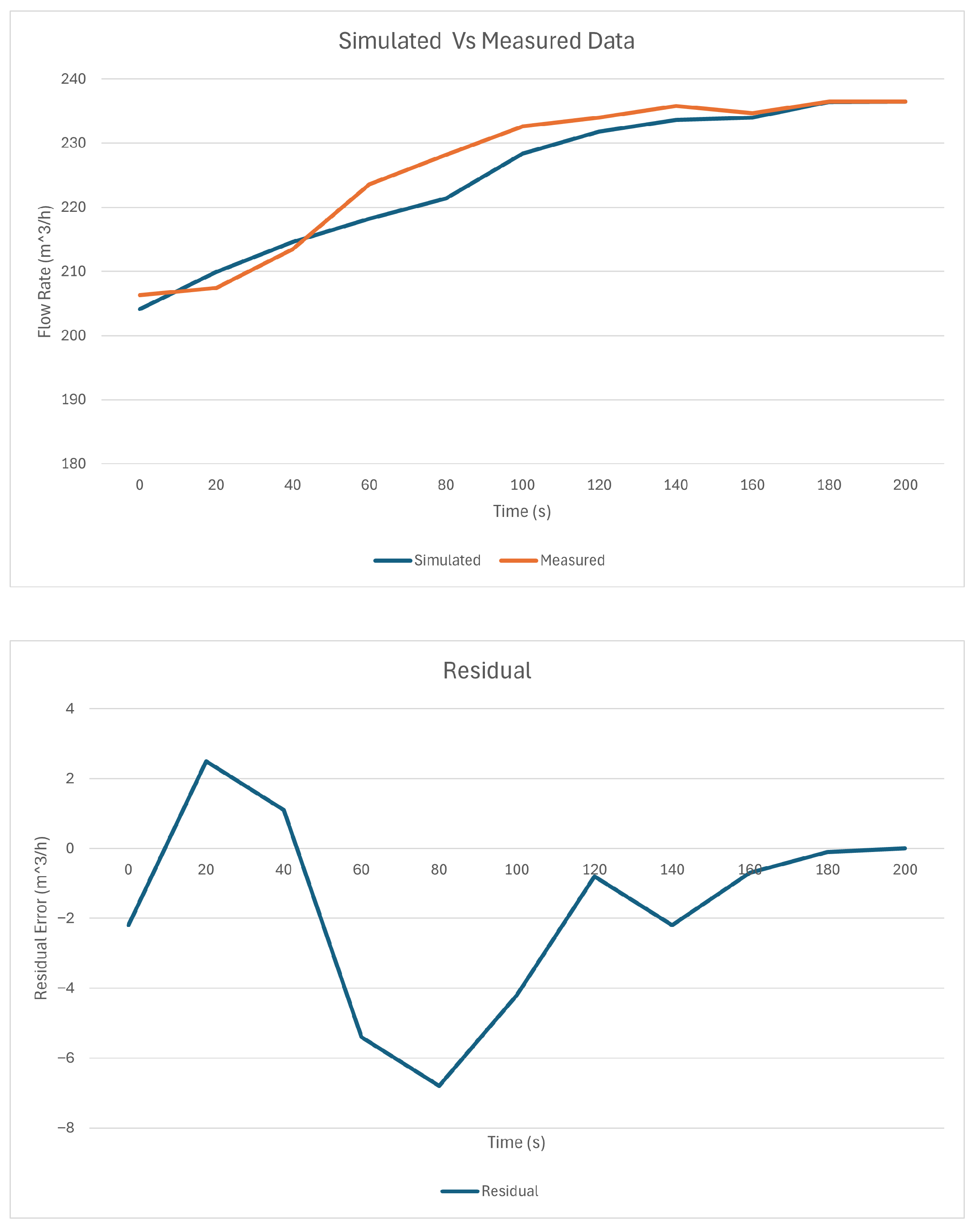
The validated model reproduced the field response with an average NRMSE of 12.6% and $R^2$ of 0.957 across three representative operating episodes. Figure 2 compares the measured and simulated flow transients for a representative setpoint step, showing close agreement in rise time, overshoot, and settling behavior.

Table 1. Validation metrics comparing simulated and SCADA flow responses.

Operating Episode	RMSE [m3/h]	NRMSE [%]	${\mathit{R}}^2$
Setpoint Step 1 (206–238 m3/h)	3.65	12.0	0.954
Setpoint Step 2 (238–270 m3/h)	4.24	13.5	0.946
Setpoint Step 3 (270–302 m3/h)	3.94	12.2	0.972
Average	3.95	12.6	0.957

summarizes the validation results for each episode.

A sensitivity analysis varying pipeline friction and fluid density by $\pm 10\%$ yielded similar NRMSE variations, confirming that the model is robust to moderate parameter uncertainty. These findings indicate that the proposed model captures the dominant closed-loop dynamics of the pumping system and is sufficiently accurate to serve as a digital testbed for subsequent adaptive control studies.

To ensure that the simulated pipeline model accurately reflects real-world system dynamics, validation data were obtained from the station’s supervisory control and data acquisition (SCADA) system. The dataset represents steady-state and transient operating conditions collected under fixed-gain PI control. Flow measurements were sampled at twenty-second intervals during normal pump station operation, encompassing a range of flow rate step changes between 200 and 300 m³/h.

These measured transients were replicated in the model, using the parameters shown in

Table 2. Simulation parameters used for the adaptive and fixed-gain controller comparison.

Parameter	Symbol	Value/Unit
Physical Parameters
Fluid density	$\rho$	700–900 kg/m3
Pump head	h	m
Pump torque	T	N · m
Moment of inertia	J	1.825 kg·m2
Nominal discharge pressure	$P_d$	100 bar
Nominal suction pressure	$P_s$	3 bar
Controller Parameters
Proportional gain (initial)	$K_p$	0.09
Integral gain (initial)	$K_i$	0.03
Forgetting factor (initial)	$\lambda$	0.99
Simulation Settings
Pump rotational speed range	$\omega$	0–3600 rpm
Flow rate range	q	0–0.185 ${\mathrm{m}}^3/\mathrm{s}$
Sampling time	$T_s$	0.1 s
Simulation duration	$t_{\mathrm{sim}}$	300 s

by applying equivalent flow rate setpoint changes, allowing direct comparison between measured and simulated responses. Key validation metrics included the coefficient of determination ($R^2$), normalized root mean square error (NRMSE), and rise time. The resulting performance values demonstrated strong model fidelity, with $R^2=0.957$, NRMSE (by range) $=12.6\%$, and rise time deviation less than 4%. These results indicate that the simulation model reliably captures the dominant hydraulic and control dynamics of the actual system, thereby providing a valid foundation for subsequent adaptive control experiments.

3. Controller Design

The controller regulates the pipeline’s discharge pressure by adjusting the centrifugal pump’s speed through a Variable Frequency Drive (VFD). Due to the pipeline dynamics’ nonlinear and time-varying nature, a self-tuning adaptive controller is used. This section outlines the design of the velocity-form controller augmented with an online variable forgetting factor Recursive Least Squares (RLS) estimator for adaptive gain tuning.

3.1. Velocity-Form PI Control Structure

The control algorithm operates in discrete time and uses the velocity form of the control law to minimize offset during gain adaptation:

$$\Delta u\left(k\right)=K_p\left(k\right)[e\left(k\right)-e(k-1)]+K_i\left(k\right)e\left(k\right)$$

(15)

$$u\left(k\right)=u(k-1)+\Delta u\left(k\right)$$

(16)

where $e\left(k\right)$ is the error between the pressure setpoint and measured pressure at time step k, and $u\left(k\right)$ is the VFD command. The gains $K_p\left(k\right)$ and $K_i\left(k\right)$ are updated at each time step using information provided by the RLS estimator.

3.2. Parameter Estimation Using RLS

The adaptive controller presented in this paper leverages Recursive Least Squares (RLS) to estimate the controller’s behavior, rather than the full nonlinear dynamics of the pipeline system. This method allows for localized, real-time adaptation of controller gains without needing an explicit model of the complex and variable fluid transport process, influenced by factors like changes in fluid density, valve transients, and pipeline friction.

The controller in velocity form is structured as follows

$$u\left(k\right)=u(k-1)+K_p\left[e\left(k\right)-e(k-1)\right]+K_i{T}_{s}e\left(k\right)$$

(17)

here, $u\left(k\right)$ is the controller output (e.g., VFD speed command), $e\left(k\right)$ is the error between setpoint and measured pressure, $T_s$ is the sampling time, and $K_p$, $K_i$ are the proportional and integral gains.

To estimate how this controller behaves under varying conditions, we represent its dynamic behavior in an autoregressive model with exogenous input (ARX) form

$$u\left(k\right)={\theta }_{1}u(k-1)+{\theta }_{2}e(k-1)+{\theta }_{3}e(k-2)+\epsilon \left(k\right)$$

(18)

where ${\theta }_1$ represents inertia or output retention, ${\theta }_2$, ${\theta }_3$ capture the effective proportional and integral behavior, and $\epsilon \left(k\right)$ is a noise or modeling error term.

The RLS algorithm minimizes the exponentially weighted least-squares cost function:

$$J\left(k\right)=\sum _{i=1}^k{\lambda }^{k-i}{\left(y\left(i\right)-{\varphi }^T\left(i\right)\theta \left(i\right)\right)}^2$$

(19)

where $0<\lambda \le 1$ is the variable forgetting factor [39], which controls the weight given to recent versus past data. A value closer to 1 emphasizes long-term memory, while a lower value increases sensitivity to parameter changes. However, simulations revealed that setting the value of $\lambda$ below $0.9$ led to rapid oscillations in ${\widehat{K}}_p\left(k\right)$ and caused algorithm instability.

The parameters $\theta ={[{\theta }_1,{\theta }_2,{\theta }_3]}^{\top }$ are estimated using the Recursive Least Squares algorithm with variable forgetting. At each time step, the regressor vector is formed as:

$$\varphi \left(k\right)={[u(k-1),e(k-1),e(k-2)]}^{\top }$$

The recursive update equations are

$$\begin{array}{cc}\hfill \widehat{\theta }\left(k\right)& =\widehat{\theta }(k-1)+K\left(k\right)\left[u\left(k\right)-{\varphi }^{\top }\left(k\right)\widehat{\theta }(k-1)\right]\hfill \end{array}$$

(20)

$$\begin{array}{cc}\hfill K\left(k\right)& ={\displaystyle \frac{P(k-1)\varphi \left(k\right)}{\lambda +{\varphi }^{\top }\left(k\right)P(k-1)\varphi \left(k\right)}}\hfill \end{array}$$

(21)

$$\begin{array}{cc}\hfill P\left(k\right)& ={\displaystyle \frac{1}{\lambda }}\left[P(k-1)-K\left(k\right){\varphi }^{\top }\left(k\right)P(k-1)\right]\hfill \end{array}$$

(22)

where $\lambda$ is the variable forgetting factor, $K\left(k\right)$ is the gain vector at time step k, and $P\left(k\right)$ is the covariance matrix of the estimator.

Once the parameter estimates ${\widehat{\theta }}_2$ and ${\widehat{\theta }}_3$ are updated, the controller gains are extracted by interpreting these parameters in the context of the velocity-form PI controller

$$\begin{array}{cc}\hfill {\widehat{K}}_p\left(k\right)& ={\widehat{\theta }}_2\left(k\right)\hfill \end{array}$$

(23)

$$\begin{array}{cc}\hfill {\widehat{K}}_i\left(k\right)& ={\displaystyle \frac{{\widehat{\theta }}_3\left(k\right)}{T_s}}\hfill \end{array}$$

(24)

These gains are then applied to the controller in real time, enabling continuous adaptation to changing pipeline dynamics. This method avoids the complexity of modeling the whole physical system by treating the controller as a dynamic system and using RLS to estimate its behavioral coefficients. This is particularly beneficial when fluid properties, pressure wave reflections, or pump dynamics are nonlinear or uncertain. The controller automatically adjusts its gain structure to match the operating environment, maintaining stability and performance across various pipeline conditions.

3.3. Stability and Robustness Considerations

While the adaptation mechanism allows the controller to respond to plant variations, stability must be preserved during transients. A lower bound is imposed on the forgetting factor $\lambda$ to prevent excessive sensitivity, and bounds are enforced on $K_p$ and $K_i$ to maintain acceptable phase and gain margins. The controller is also tested under worst-case transients and variable density profiles to evaluate robustness (see Section 4).

4. Simulation Results

To evaluate the performance of the proposed self-tuning adaptive controller, a series of simulations was conducted using a nonlinear dynamic model of an induction motor-driven centrifugal pump connected to a pipeline with a downstream valve. The primary objective is to assess the controller’s ability to adapt to changing fluid densities and respond effectively to overpressure scenarios.

4.1. Simulation Setup

The simulation environment was developed in MATLAB 2023b, with a fixed sample time of $T_s=0.1$ s. The plant includes an induction motor model based on electrical torque-speed characteristics, a centrifugal pump with a nonlinear head-flow curve, a rigid pipeline transporting fluids of varying densities (700–900 kg/m³), and a downstream valve capable of closure to simulate overpressure conditions.

The controller is implemented in both fixed-gain and adaptive configurations, where the adaptive version updates the controller gains in real time using Recursive Least Squares (RLS) estimation.

4.2. Case Study 1: Step Change in Fluid Density

To test the controller’s responsiveness to changing pipeline conditions, the fluid density was stepped from 700 kg/m³ to 900 kg/m³ at $t=200$ s.

4.2.1. Fixed-Gain Response to a Change in Fluid Density

Figure 3 shows that the fixed-gain controller exhibits overshoot and oscillations due to the mismatch between controller tuning and the new process dynamics. The pump takes longer to stabilize at the desired setpoint, and with no intervention by the operator, the discharge pressure reaches $115.7$ bar, which results in a $113.4\%$ overpressure. Figure 4.

4.2.2. Adaptive Controller Response to a Change in Fluid Density

Figure 5 and Figure 6 demonstrate that the adaptive controller successfully tunes the gains in real time. The response shows minimal overshoot and a faster settling time as the controller compensates for the change in fluid density. The maximum pressure at the pump’s discharge was $103.6$ bar, resulting in a $101.6\%$ overpressure Figure 7.

4.3. Case Study 2: Valve Closure and Overpressure Event

This scenario simulates a downstream valve closure at $t=250$ s, initiating a pressure wave toward the pump.

4.3.1. Fixed-Gain Response to a Overpressure Event

As seen in Figure 8 and Figure 9, the fixed-gain controller cannot adapt quickly to the pressure spike, resulting in prolonged overpressure conditions. In this scenario, the maximum pressure at the pump’s discharge was $109.6$ bar, resulting in a $107\%$ overpressure. This highlights the potential risk of pipeline integrity breaches.

4.3.2. Adaptive Controller Response to a Overpressure Event

The adaptive controller, shown in Figure 10, Figure 11 and Figure 12, detects the deviation and quickly adjusts its gains to reduce the pressure added by the pump. The maximum pressure at the pump’s discharge was $103.1$ bar, resulting in a $101\%$ overpressure. This mitigates the overpressure effect and reduces the system’s exposure to damaging pressure levels.

4.4. Quantitative Performance Comparison

Table 3. Performance Comparison of Fixed vs. Adaptive PI Controllers.

Metric	Fixed-Gain	Adaptive RLS	Improvement
Rise Time (s)	120	0.70	99.4%
Overshoot (%)	1.91	1.30	31.9%
Settling Time (s)	1.6	1.5	6.25%
Energy Use (kWh)	1.39	2.25	−61.8%

summarizes key performance metrics for both controller types. The adaptive controller consistently outperforms the fixed-gain controller in rise time, overshoot, and settling time, but not energy efficiency.

5. Discussion

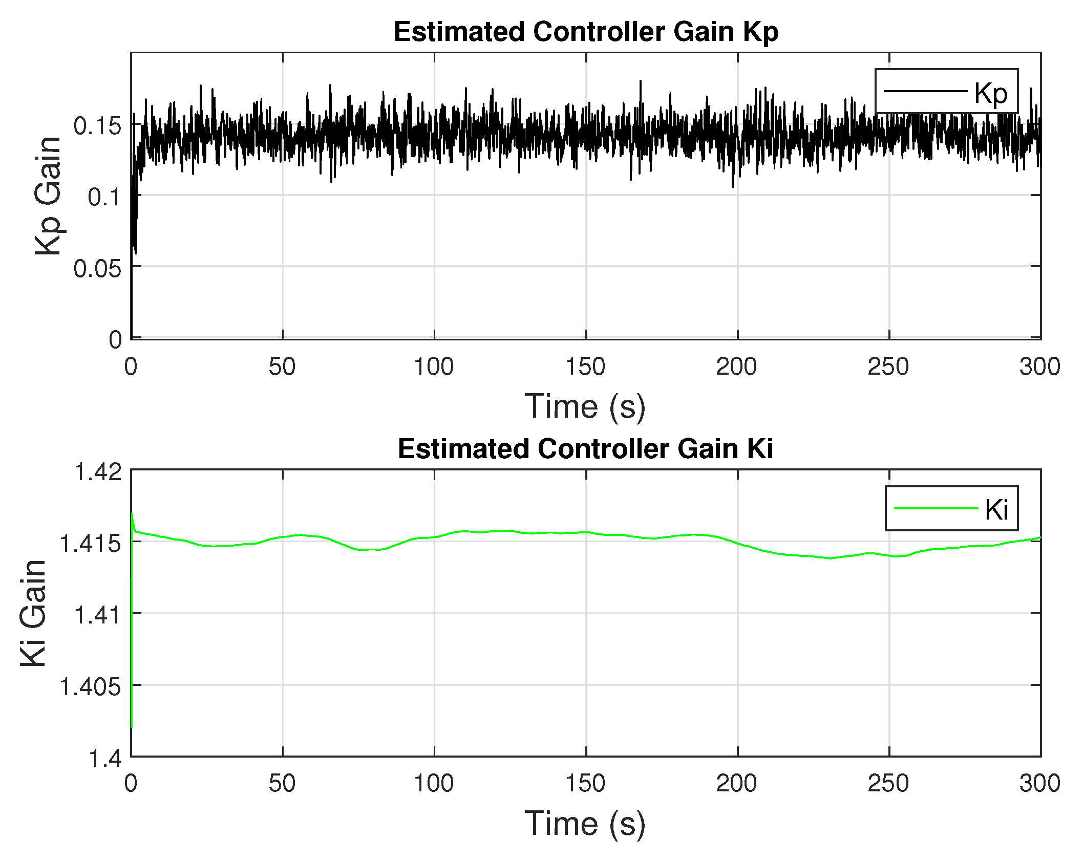
The simulation results in Section 4 demonstrate the effectiveness of the RLS-based self-tuning controller in dynamically adjusting to changing system conditions. The controller successfully modified its gains in real time to maintain setpoint tracking and prevent system instability during steady-state operations and transient disturbances.

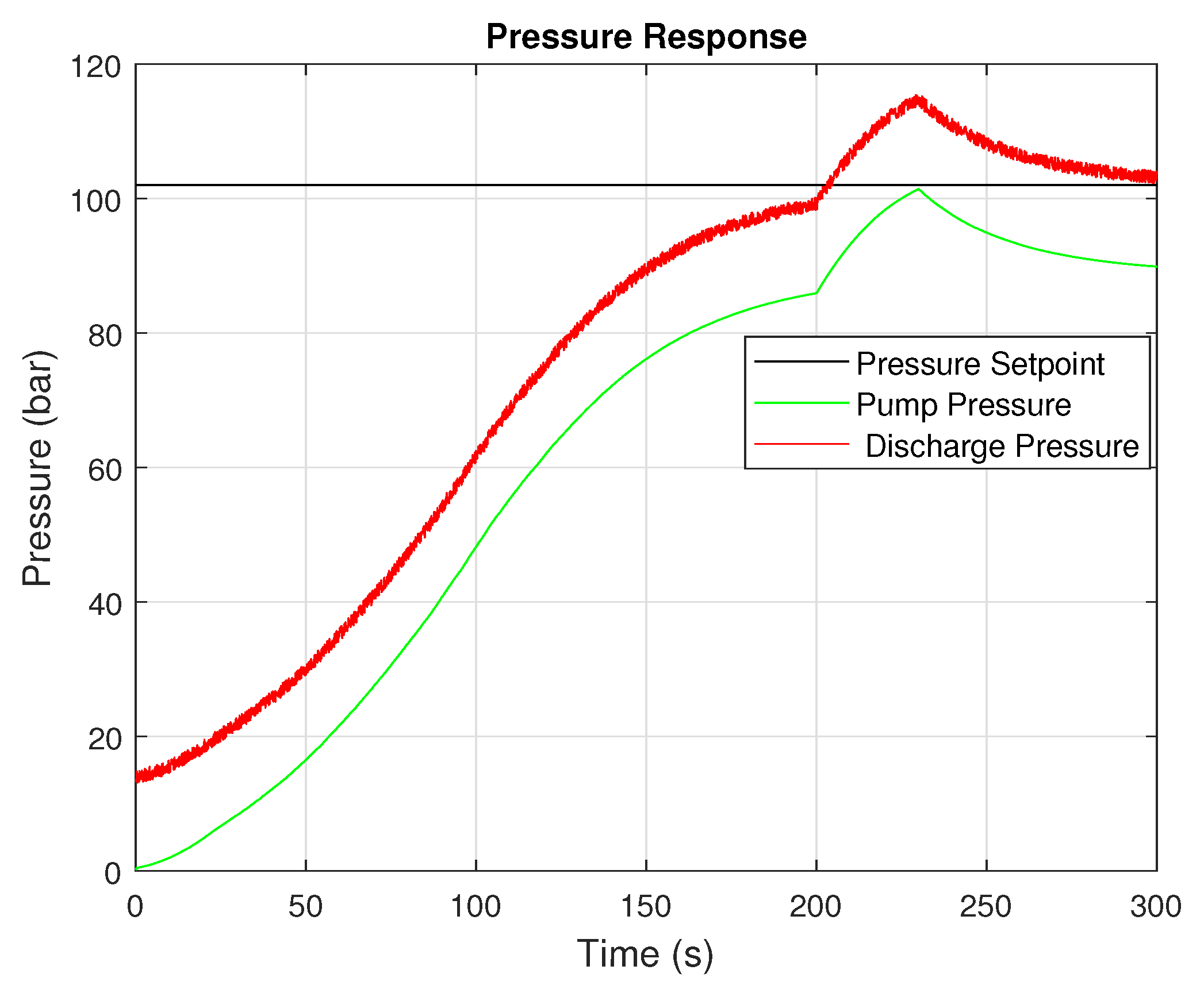
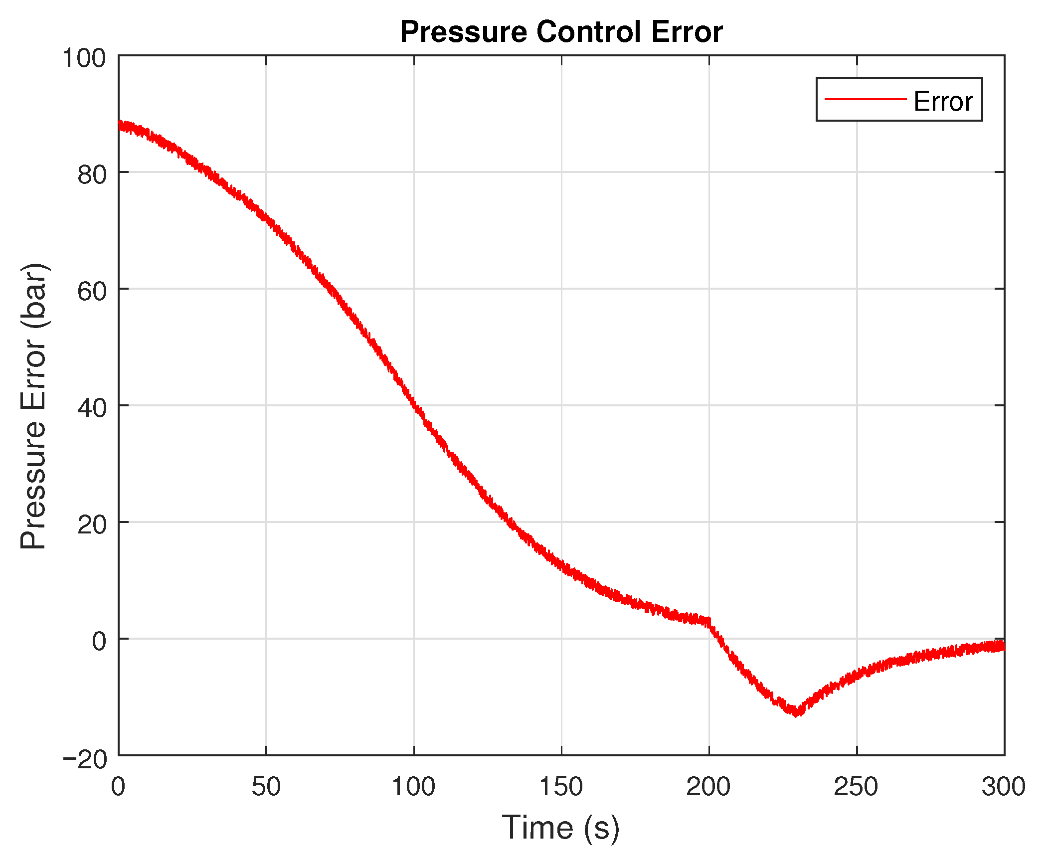
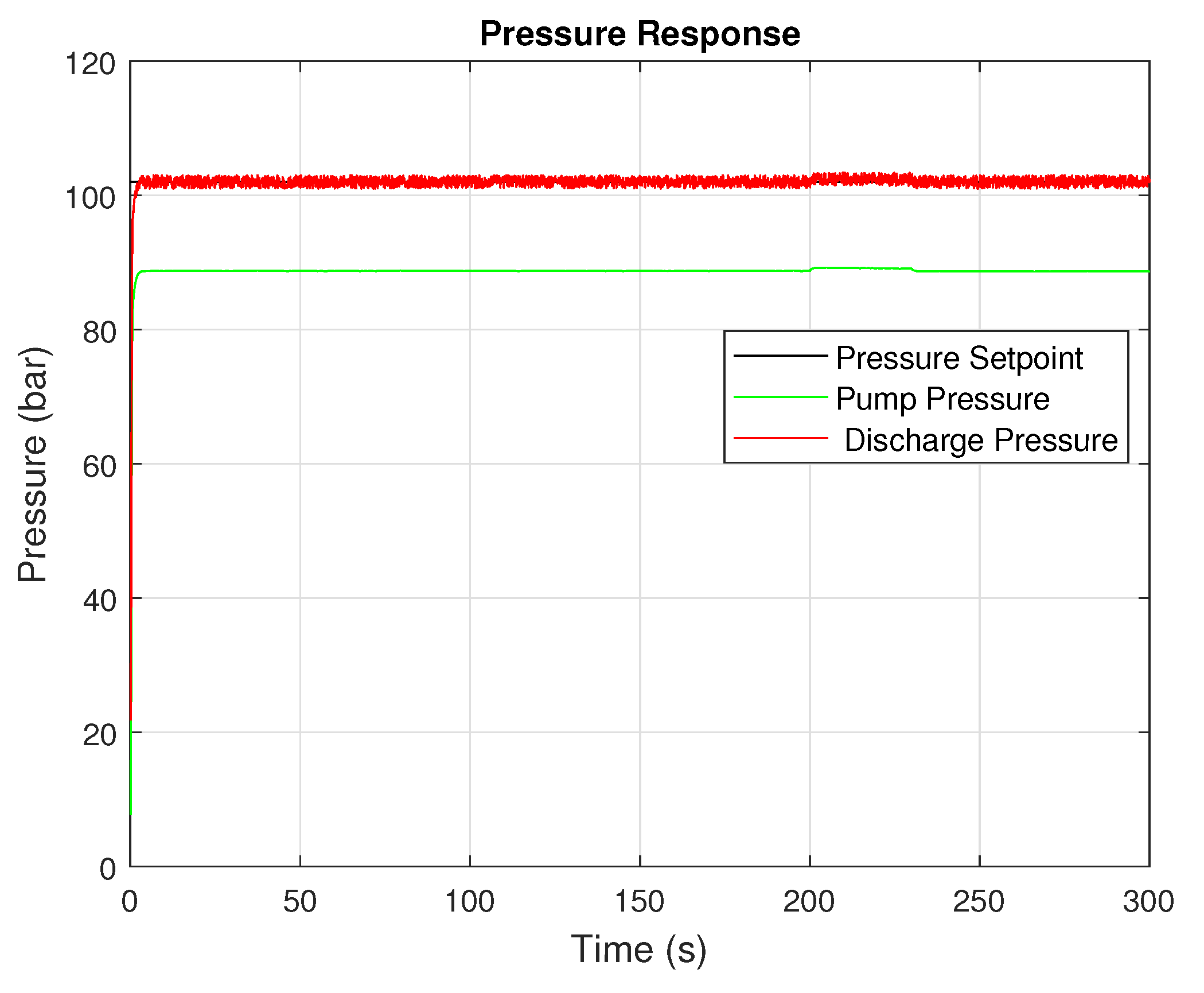
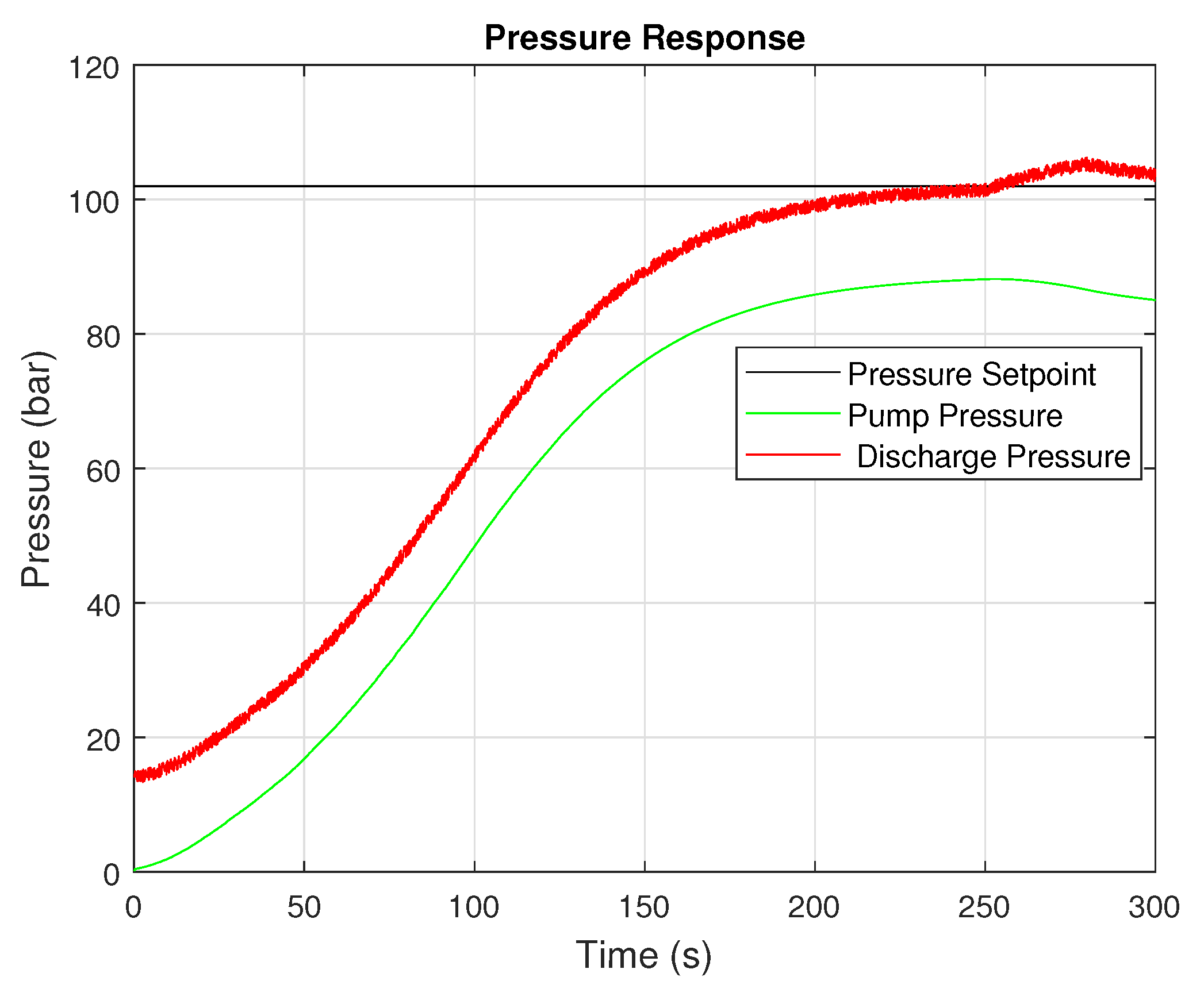
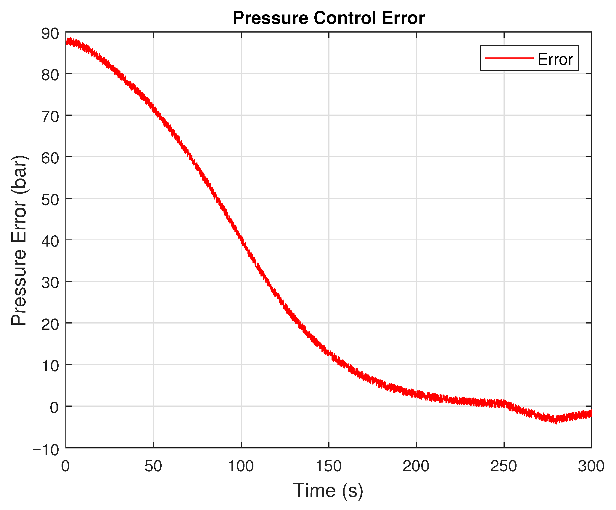
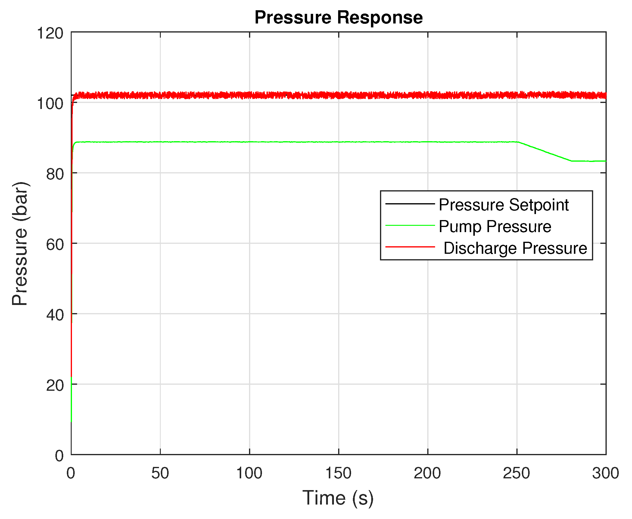
For example, in the scenario involving a step change in fluid density, the adaptive controller reduced the settling time and overshoot compared to the fixed-gain implementation and reduced the maximum pressure from $115.7$ bar to $103.6$ bar. In valve closure simulations, the controller responded quickly to the induced pressure surge, dampening the oscillations and keeping the pressure below the critical threshold, reducing the maximum pressure from $109.6$ bar to $103.1$ bar.

The adaptive controller maintained desired performance across a broader range of operating conditions without requiring manual retuning. This is particularly beneficial for pipeline applications where fluid properties and system dynamics change frequently due to batching, elevation shifts, or unexpected disturbances.

By continually updating the internal process model through the RLS algorithm, the controller could anticipate and compensate for changes in the plant’s gain and time constant. This eliminated the need for pre-programmed gain schedules or conservative tuning that compromises performance.

A significant contribution of the adaptive controller is its ability to mitigate overpressure conditions, a known contributor to pipeline failure and safety incidents. By maintaining more consistent control during pressure wave events, the system stayed within safe operational boundaries for a more extended portion of the simulation.

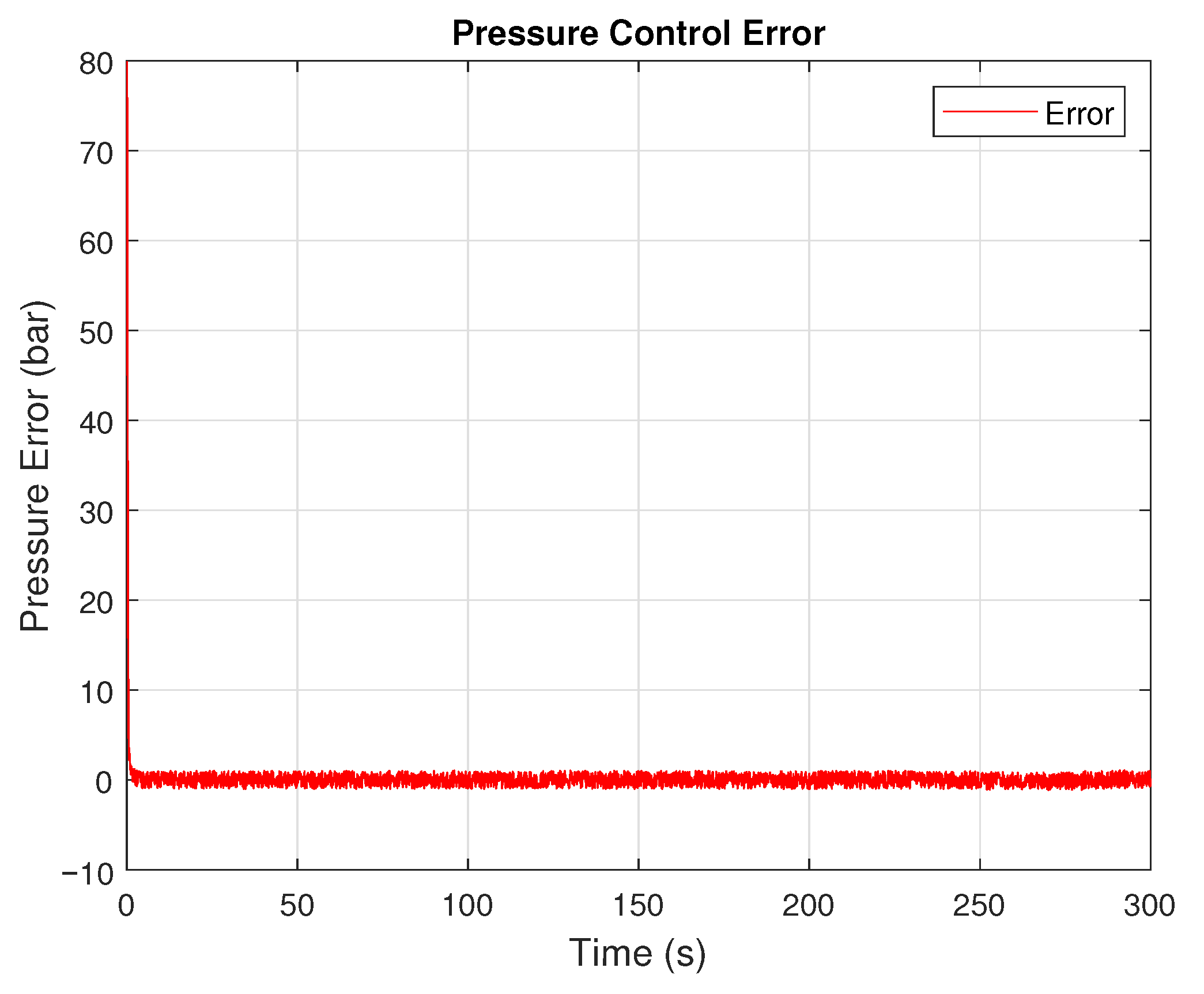
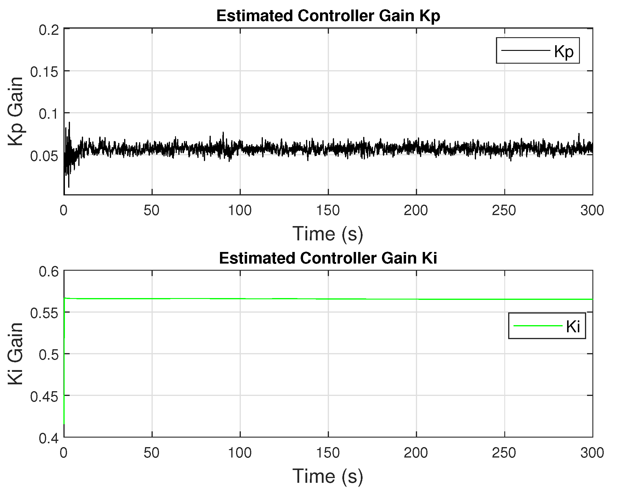
The results indicate that the adaptive controller required greater energy input compared to the fixed-gain PI controller, consuming approximately 61% more total energy over the same operating interval. This increase is directly attributable to the enhanced control effort needed to achieve faster dynamic response and reduced transient error. The self-tuning mechanism of the RLS-based controller continuously updates the proportional ($K_p$) and integral ($K_i$) gains in response to pressure deviations, resulting in more aggressive actuator commands, particularly during rapid load or setpoint changes. While this adaptive behavior enables the system to reach the target pressure in less than one second (compared to 120 s for the fixed controller), it also leads to higher pump torque demand and, consequently, increased energy consumption. These results illustrate a fundamental trade-off between dynamic performance and energy cost, emphasizing that the adaptive controller improves responsiveness and tracking accuracy at the expense of higher control activity. Future work will focus on incorporating multi-objective adaptation criteria to balance transient performance and energy efficiency.

5.1. Limitations and Considerations

Despite the promising results, some limitations are noted. The RLS estimator assumes a persistent excitation in the input signal, which may not always be present in normal pipeline operations. In minimal input variation, parameter convergence could slow, delaying adaptive response. Furthermore, this approach assumes an approximation of the local dynamics and nonlinear behaviors, unmodeled disturbances, or actuator saturation may challenge the adaptive strategy. Also, the control-oriented plant model used in this study incorporates the dominant hydraulic and pump dynamics required for controller development, but it relies on several simplifying assumptions that may affect quantitative agreement with field behavior. Key simplifications include a lumped-parameter representation of the pipeline (rather than a full method-of-characteristics solution), idealized valve actuation models, and steady-state pump curves with simplified transient mapping from shaft speed to heads. These approximations could result in a reduced high-frequency content and may underpredict local peak pressures and arrival-time precision during very fast transients. In recognition of these limitations, results are reported with conservative performance claims.

5.2. Relation to Broader Control Strategy

This initial single-loop adaptive control forms the foundation for more complex control hierarchies. The conceptual road map shows that this layer can be extended to multi-loop coordination via Q-learning and inter-station negotiation via cooperative game theory. The robust performance observed here justifies expanding the approach to more complex configurations and higher-level control objectives.

6. Conclusions

This study presented a self-tuning adaptive controller for centrifugal pump regulation in a pipeline system using a variable forgetting factor Recursive Least Squares (RLS) algorithm for real-time process identification. The control strategy was implemented within a velocity-based loop and validated under varying product densities and transient pressure disturbances, including valve closure events.

Simulation results confirmed significant performance improvements over conventional fixed-gain PI control. The adaptive controller reduced peak overshoot by 31.9% and settling time by 6.25%. During simulated overpressure conditions, transient overpressures were reduced by approximately 6%, reducing the peak pressure observed from $109.6$ bar to $103.1$ bar. Similar results were seen during product changes where the density of the fluid increased from 700 to 900 $\mathrm{kg}/{\mathrm{m}}^3$. Smoother actuator dynamics and reduced oscillatory behavior were also observed.

The findings demonstrate that while the self-tuning RLS-based controller achieved a substantially faster pressure response and improved tracking accuracy, these benefits were accompanied by increased energy consumption due to higher control effort. This outcome highlights an inherent trade-off between dynamic performance and energy cost in adaptive control of centrifugal pumps. Future research will focus on refining the adaptation law to incorporate energy-aware or multi-objective optimization criteria that can achieve an improved balance between responsiveness and efficiency.

These results demonstrate that online RLS-based parameter adaptation enhances loop robustness and pressure stability across a wide operating range without requiring manual gain retuning. The improved dynamic response also contributes to safer and more efficient pipeline operations.

This work validates the feasibility of localized adaptive control for pump-driven pipeline systems and establishes a foundation for hierarchical extensions. Future studies will focus on supervisory-level coordination within multi-loop pump stations and game-theoretic strategies for inter-station energy balancing, advancing toward an integrated intelligent control framework for modern fluid transport networks.