Abstract
Infrasound leakage signals, with low propagation energy loss, are ideal for long-distance and small leakage detection but suffer severe background noise interference. Existing wavelet denoising methods using traditional soft/hard threshold functions face critical limitations: soft thresholds introduce constant deviation, while hard thresholds cause discontinuities, both leading to suboptimal noise reduction for infrasound signals—this gap hinders accurate leakage detection. To address this, we propose a wavelet denoising method with an improved threshold function, analyze its process via the Mallat algorithm, and prove its continuity and convergence. Comparative experiments on infrasound leakage data show that, at the optimal decomposition level, our method reduces RMSE by 41.19% and increases SNR by 5.1326 dB compared to the soft threshold method; versus the hard threshold method, RMSE decreases by 34.65% and SNR increases by 4.2148 dB. It also separates background noise more thoroughly in time–frequency domains, demonstrating strong feasibility for pipeline infrasound leakage detection.
1. Introduction
The pipeline network plays an important role in the industrial, civil, and military fields. Adverse environmental conditions or human-induced damage can easily lead to pipeline leakage. This not only wastes resources and pollutes the environment, but also threatens the safety of operators. Therefore, effective leakage detection of existing pipeline network status has gradually become an urgent problem to be solved in the pipeline transport industry [1,2]. Common pipeline leakage detection methods mainly include the distributed optical fiber sensor method, magnetic flux leakage detection method, crawling robot detection method, model-based detection method, negative pressure wave-based method, and infrasound-based detection method [3,4]. The leakage detection method based on infrasound features low signal frequency, minimal energy loss during transmission, and signal independence from fluid density and pressure, making it suitable for detecting small-flow leakage. The disadvantage is that infrasonic signals are easily interfered with by noise, so the key problem of using the infrasound method for leakage detection is the noise reduction processing of the original signal [5,6].
However, denoising infrasound signals is particularly challenging due to their unique characteristics, which make existing methods less effective. First, infrasound signals (typically 0.0001–20 Hz) lie in an extremely low-frequency band, far below the range targeted by most conventional denoising methods (designed for mid-high frequency signals >20 Hz). This frequency mismatch leads to insufficient frequency resolution, making it hard to distinguish valid infrasound from noise [7]. Second, infrasound signals often suffer from an extremely low signal-to-noise ratio (SNR, usually <0 dB) due to weak propagation and intense environmental interference (e.g., atmospheric turbulence and sensor vibration), which causes traditional threshold-based or filtering methods to misjudge valid components as noise [8]. Third, the frequency and time domains of infrasound noise overlap heavily with those of leakage signals, rendering methods relying on feature differences (e.g., adaptive filtering and empirical mode decomposition) ineffective in separation [9].
Common signal denoising methods mainly include the following: the Fourier transform method, adaptive filtering method, empirical mode method, sparse decomposition method, blind source separation method, and wavelet analysis method. Among them, wavelet transform is a typical nonlinear analysis method. At present, there are three main denoising methods based on wavelet analysis: the wavelet mode extremum method, spatial correlation method, and wavelet threshold function analysis method [10,11]. The wavelet threshold denoising method has the advantages of a simple algorithm, reliable operation, and fast operation speed, and has become a research hotspot and is widely used. Donoho and Johnstone [12,13] proposed a wavelet threshold denoising algorithm using hard and soft threshold function methods; this algorithm is simple to implement but suffers from problems of discontinuity points and constant deviation. Gao and Bruce [14] improved the hard and soft threshold methods and proposed a semi-soft threshold denoising analysis method. This method achieves a better denoising effect than the hard and soft threshold methods, but the determination of parameters is more difficult. Luisier et al. [15] proposed a wavelet threshold improvement method using a genetic algorithm. Li et al. [16] proposed a hybrid particle swarm optimization (PSO)-based wavelet adaptive threshold estimation algorithm. The above two methods have complex operation processes that require multiple iterations; their inherent defect is a slow convergence rate, and the optimization of discrete information tends to fall into local optimal solutions.
Over the past five years, research on the wavelet threshold denoising method has focused on addressing the challenges of processing low-frequency, low-signal-to-noise ratio (SNR) signals, proceeding along three main directions: threshold function optimization, multi-method fusion, and integration with deep learning.
In terms of threshold function optimization, although progress has been made—such as the development of parameter-adjustable continuous functions and dynamic strategies combined with voice activity detection—these achievements lacked customized adaptation for the ultra-low frequency band specific to infrasound. A recent 2024 study optimized threshold selection for acoustic signals by proposing an adaptive threshold calculation method integrated with an improved simulated annealing algorithm; this method reduced reliance on manual parameter tuning and demonstrated stronger robustness for signals with SNR < 5 dB, laying a foundation for low-frequency acoustic denoising [17]. However, it was not tailored to the 0.0001–20 Hz ultra-low-frequency range of pipeline infrasound, leading to suboptimal retention of weak leakage features.
In the area of multi-method fusion, schemes like improved ensemble empirical mode decomposition (MEEMD)-time-varying Vector Autoregressive Moving Average (VARMA) model and wavelet packet-F-x-K-L (frequency–space Karhunen–Loève) joint scheme have improved denoising performance but were plagued by high computational complexity [18]. Recent fusion strategies targeting pipeline infrasound have shown promising results. A 2023 study combined improved complementary EEMD (ICEEMD) with fine composite multiscale entropy for urban nonmetallic pipeline infrasound, increasing the SNR from 13 to 25 dB and reducing the average RMSE from 24.82% to 3.39% [19]; however, its entropy-based component screening led to unavoidable loss of subtle signal details. A 2024 work proposed a Beluga Whale Optimization (BWO)-optimized Variational Mode Decomposition (VMD) combined with wavelet thresholding to solve VMD’s parameter sensitivity issue. Compared to GWO/SSA-optimized schemes, its SNR was improved by 1.27–2.01% [18], but the dual-module fusion increased computation time by 40% compared to single-wavelet methods. Additionally, a 2024 patent applied improved adaptive optimal kernel time–frequency distribution (AOK-TFR) to pipeline infrasound processing, effectively suppressing cross-interference in time–frequency domains [20], yet it failed to resolve frequency overlap between infrasound and environmental noise.
In the direction of deep learning integration, combining CNNs/autoencoders with wavelet thresholding enabled accurate denoising in low-SNR scenarios; however, this approach relied on scarce labeled datasets and suffered from the “black box” limitation of deep learning. To date, no fully validated deep learning-based solutions for pipeline infrasound denoising have been reported, as existing models are either designed for other low-frequency signals (e.g., seismic and EEG) or lack generalization to industrial pipeline scenarios [18].
Overall, while existing studies have enhanced the method’s performance, they have failed to fully resolve the unique challenges in processing infrasound pipeline leakage signals—either due to frequency adaptation mismatch, excessive computational cost, or limited generalization—creating an urgent need for a targeted, efficient, and interpretable solution. Given that wavelet threshold denoising inherently excels at band-separated signal processing—a key feature matching the infrasound—noise frequency distribution (infrasound <20 Hz vs. high-frequency noise)—we chose to optimize this method to fill the above research gap.
The wavelet threshold denoising method is very effective when the signal and noise frequency bands are separated from each other [21,22]. The infrasound signal is below 20 Hz, and the noise is distributed in the high-frequency range, so this method is very suitable for processing infrasound leakage signals [23,24]. In this paper, a wavelet denoising algorithm with an improved threshold function is proposed to address the defects of the classical wavelet denoising method, and it is applied to signal denoising for pipeline infrasound sensors.
This study makes three key contributions: (i) It designs an improved threshold function tailored to infrasound leakage signals, addressing the discontinuity of hard thresholds and constant deviation of soft thresholds simultaneously. (ii) It theoretically proves the continuity and convergence of the improved function, providing a solid basis for its effectiveness. (iii) It validates the proposed method through comparative experiments, demonstrating that it outperforms traditional threshold methods in SNR, RMSE, and time–frequency noise separation, thus enhancing the feasibility of infrasound-based pipeline leakage detection in industrial scenarios.
The structure of this paper is arranged as follows: Section 1 (Introduction) elaborates on the research background of pipeline leakage detection, the advantages and noise challenges of the infrasound method, sorts out the limitations of existing denoising methods, and clarifies the research objectives. Section 2 (Materials and Methods) is divided into three subsections: Section 2.1: Wavelet Threshold Denoising Process introduces the process of wavelet threshold denoising; Section 2.2: Classical Threshold Function and its Limitations analyzes classical threshold functions and their limitations; Section 2.3 Improved Threshold Function Algorithm details the design idea of the improved threshold function algorithm, as well as the theoretical proofs of its continuity and convergence; Section 3 (Experiment) is divided into two sections: Section 3.1: Establishment of Experimental Platform explains the construction of the experimental platform; Section 3.2: Analysis of Leakage Infrasound Signal elaborates on the acquisition and analysis process of leakage infrasound signals and the setting of traditional comparative methods. Section 4 (Results and Discussion) conducts comparative analyses and discussions on the denoising effects of the improved method and traditional threshold methods from the dimensions of signal-to-noise ratio (SNR), root mean square error (RMSE), and time–frequency domain features. Section 5 (Conclusion) summarizes the research results, points out the limitations, and proposes future research directions. Finally, there is the References section.
2. Materials and Methods
2.1. Wavelet Threshold Denoising Process
Define a one-dimensional noisy signal, assuming there is a total of N-1 noisy signals, as shown in Formula (1):
In the formula: —raw signal, —real signal, and —noise deviation coefficient, —noise signal.
Due to the influence of various noise signals, extracting signal must rely on mathematical methods for noise reduction. Wavelet analysis can effectively analyze the time–frequency characteristics of signals; thus, it is often regarded as the best choice for field signal processing. Figure 1 shows a schematic diagram of the processing method for one-dimensional noisy signals.
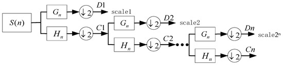
Figure 1.
Schematic diagram of wavelet signal decomposition.
In Figure 1, S(n) is a noisy signal, which can be decomposed into a nearly stationary signal and a noisy signal layer by layer. For example, the first decomposition yields C1 (a nearly stationary signal) and D1 (a noisy signal); C1 continues to decompose according to the accuracy requirements until the requirements are met. In this figure, C1, C2,…, Cn are the low-frequency signals obtained via layer-by-layer decomposition, characterized by low frequency and relative stability, and they contain the main useful signals. D1, D2,…, Dn are high-frequency signals, with relatively few useful signals in this part. The amplitude of the wavelet coefficients in the useful signal part is relatively larger, while the amplitude of the corresponding coefficients of the noise is smaller. Therefore, the threshold method can be used to process the wavelet coefficients: retain the high-amplitude useful signals and filter out the high-frequency, low-amplitude noise signals. The signal reconstruction steps are the reverse of decomposition, as shown in Figure 1. Specifically, Cn − 1 is first reconstructed from Cn and Dn, then Cn − 2 is reconstructed from Cn − 1 and Dn − 1, and finally S(n) is reconstructed from C1 and D1. After signal reconstruction, a reconstructed signal that is close to the real signal can be obtained.
Based on the above analysis, the wavelet denoising process can be carried out according to Figure 2.
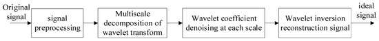
Figure 2.
Flow chart of wavelet threshold denoising.
2.2. Classical Threshold Function and Its Limitations
The selection of a threshold function has a great influence on the effect of wavelet denoising, and constructing an excellent threshold function is the key to ideal wavelet analysis [25,26]. The basic idea of the threshold function-based denoising method is that of obtaining a series of wavelet coefficients after wavelet decomposition of the original signal, determining the denoising threshold, processing the wavelet coefficients according to certain functional rules, and using the processed wavelet coefficients to reconstruct the signal. At present, the commonly used threshold determination methods mainly include the hard threshold method, the soft threshold method, and the semi-soft threshold method [27,28].
- (1)
- Hard threshold method
The function expression of the hard threshold method is
Here, λ denotes the denoising threshold, represents the original wavelet coefficient, and is the processed wavelet coefficient. According to Equation (2), wavelet coefficients larger than the threshold are retained, while those that are smaller are all set to zero.
- (2)
- Soft threshold method
The functional expression of the soft threshold method is
According to Equation (3), the basic idea of the soft threshold method is as follows: all wavelet coefficients below the threshold are set to zero, and those greater than or equal to the threshold have the threshold value subtracted from them and are retained.
- (3)
- Semi-soft threshold method
The function expression of the semi-soft threshold method [29] is
According to Formula (4), the basic idea of semi-soft threshold method is as follows: when is greater than , its processing mode is the same as that of the hard threshold function; when is between and , it approximates the soft threshold function. When , it corresponds to the hard threshold method; when approaches infinity, it corresponds to the soft threshold method. This method is based on the soft and hard threshold methods, and its denoising effect is excellent. However, the determination of the two thresholds is difficult, so it is rarely used in practical applications.
Hard and soft threshold methods are the most widely used in denoising processing, but they also have significant drawbacks. As shown in Figure 3a, the wavelet coefficients processed by the hard threshold method are discontinuous at point , resulting in oscillation after signal reconstruction; as shown in Figure 3b, the soft threshold method yields continuous signals on the vertical axis, but this comes at the cost of sacrificing the accuracy of threshold-scale data, leading to a significant deviation between the reconstructed signal and the real signal [30].
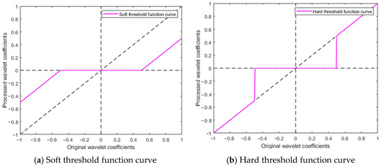
Figure 3.
Function curves of soft thresholding and hard thresholding.
2.3. Improved Threshold Function Algorithm
To construct a threshold function with good denoising effect, the following requirements should be met: the threshold function is continuous to avoid the pseudo-Gibbs phenomenon; the function structure is simple and adjustable via parameter control; the function has the property of high-order differentiability for ease of calculation; the curve near the threshold point is smooth to prevent oscillation of the reconstructed signal.
These requirements precisely highlight the limitations of classical threshold functions: the hard threshold function, though simple in structure, exhibits step discontinuity at the threshold point, easily inducing pseudo-Gibbs oscillations and failing to satisfy high-order differentiability; the soft threshold function, despite achieving continuity, has a constant shrinkage bias and an abrupt change in derivative at the threshold point, failing to achieve a smooth transition. Both are difficult to adapt to the denoising requirements of infrasound signals characterized by “low frequency, weak features, and low signal-to-noise ratio (SNR)”.
To address this, based on analyzing the advantages and disadvantages of hard and soft threshold methods, this paper designs an improved threshold function by introducing an exponential smooth transition term to specifically solve the above issues.
This improved threshold function is specifically constructed as follows:
Herein, adopts a fixed threshold as follows:
In the formula: —wavelet threshold, —adjustment coefficient, —noise standard deviation, and N—signal length
It can simultaneously achieve continuity of both function value and first-order derivative at the threshold points ±λ, completely eliminating oscillations caused by discontinuity. The shrinkage amount is dynamically adjusted with the amplitude of coefficients—for weak signals close to the threshold (e.g., infrasound leakage features), small-amplitude shrinkage is adopted to reduce loss, while for strong signals far from the threshold, the shrinkage amount approaches 0 to avoid constant bias. The introduced adjustment parameter α is directly related to the main frequency characteristics of infrasound (the larger α is, the narrower the transition band, adapting to high-frequency infrasound; the smaller α is, the wider the transition band, adapting to ultra-low-frequency infrasound), thus solving the problem of vague physical meaning of parameters.
For different noisy signals, the optimal noise reduction effect can be obtained by selecting appropriate adjustment coefficients via this function. The continuity and convergence of this function are now proved as follows.
- (1)
- Proof of continuity
First, translate the function to eliminate the interval where the function is identically zero −. Let , when , let (here , corresponding to the original upper threshold boundary ). When , let (here , corresponding to the original lower threshold boundary ). Through this substitution, the threshold boundaries of the original function are converted to the zero point of the new variable x, facilitating the analysis of continuity. From this, the following function is derived:
When , the original function becomes
Find the limit of the above formula at 0: when , find the limit of at 0:
Similarly, when , it can be deduced that the limit of at 0 is also 0. Therefore, when , ; when , The new threshold function is C0 continuous at .
The following proves that the new threshold function satisfies C1 order continuity at position .
When , the derivative of is
When , the derivative of is
According to Formulas (10) and (11), the derivative of at is
From Formula (12), it can be seen that the new threshold function has the same first-order derivative value at point , so the new threshold function satisfies C1 order continuity.
To provide an intuitive interpretation, the C0-order continuity (continuity of function values) at the threshold ensures there is no abrupt “jump” when processing wavelet coefficients. For infrasound denoising, this directly translates to avoiding pseudo-Gibbs oscillations—an artifact that severely degrades signal smoothness, especially for the low-frequency, inherently smooth infrasound signals. The C1-order continuity (continuity of first-order derivatives) further guarantees a seamless transition near the threshold, eliminating subtle “jerks” or discontinuities in the denoised signal. This is crucial for preserving the weak, low-amplitude features of infrasound leakage (e.g., small-flow pipeline leakage), as abrupt transitions would otherwise distort these critical details.
- (2)
- Proof of convergence
If , then ;
If , then ;
If , then ; if , then .
The adjustment factor α is introduced, so that the improved threshold function can be adjusted according to different signal characteristics, which makes the function model more flexible and improves the adaptability of the function. The selection of the adjustment parameter α follows two core principles: aligning with the inherent characteristics of infrasound signals and ensuring methodological reproducibility, and is implemented through two steps. First, the initial adjustment direction of α is determined based on the main frequency distribution of infrasound—for signals with lower main frequencies, α is adjusted to broaden the threshold transition band to adapt to the slow variation in ultra-low-frequency components, while for signals with relatively higher main frequencies, α is adjusted to narrow the transition band to avoid over-smoothing high-frequency infrasound details. Second, the initial range of α is defined by referencing the “parameter–function performance” correlation framework from studies on low-frequency weak signal denoising (consistent with infrasound scenarios), rather than directly adopting specific numerical ranges, to reduce the blindness of subsequent optimization. Figure 4 shows the comparison curve of wavelet coefficient processing results under different adjustment coefficients.
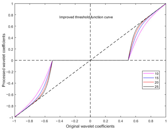
Figure 4.
Improved threshold function curve.
So, the Asymptote of is . That is to say, as increases, continuously approaches . The continuity of the new threshold function solves the signal oscillation problem of the hard threshold method, and its convergence solves the problem of constant deviation between and in the soft threshold function method.
The signal reconstructed by the hard threshold method has oscillation issues, and its discontinuity can easily lead to the pseudo-Gibbs phenomenon. The reconstructed signal using the soft threshold method is smooth and continuous, but its constant deviation leads to distortion in the reconstructed results. The improved wavelet denoising method based on a threshold function proposed in this paper solves the problems of signal oscillation and constant deviation, and makes up for the shortcomings of the traditional hard and soft threshold function methods.
Intuitively, the convergence property () means that wavelet coefficients with large amplitudes (whether they are strong infrasound signal components or high-amplitude noise) are preserved without unnecessary shrinkage. For infrasound denoising, this is vital: strong valid signals (e.g., intense leakage events) are not artificially attenuated (unlike in soft thresholding, which introduces constant bias), while high-amplitude noise is still filtered out by the threshold logic. In practice, this balances noise suppression and signal fidelity, ensuring both weak and strong infrasound features are retained intact during denoising.
3. Experiment
3.1. Establishment of Experimental Platform
The experimental platform consists of the power system, the pipeline valve control system, and the monitoring system. The power system includes the water pump and the water storage device. The pipeline valve control system includes the testing pipelines, leakage devices, and valves. The monitoring system includes the data acquisition device (Advantech USB-5856, Advantech Co., Ltd., Taipei City, Taiwan Province, China), the infrasound sensor (Model CS-100, The 3rd Research Institute of China Electronics Technology Group Corporation (CETC), Beijing City, China), and the monitoring computer (Inspur NF5280M6, Inspur Electronic Information Industry Co., Ltd., Jinan City, Shandong Province, China). This platform can provide leakage monitoring of the water medium under different pipeline pressures and leakage aperture sizes. Medium flow path: reservoir→water pump (Model ISG100-200, Shanghai Kaiquan Pump Co., Ltd., Shanghai, China)→water storage tank (homemade, 500 L)→butterfly valve (Model D371X-16, Zhejiang Dunan Valve Co., Ltd., Wenzhou, Zhejiang, China)→rubber hose (Food-grade EPDM, Hebei Huafeng Rubber Products Co., Ltd., Cangzhou, Hebei, China)→the 1# ball valve (Model Q41F-16P, Shanghai Huifeng Valve Group Co., Ltd., Shanghai, China)→outdoor pipeline→the 2# ball valve (same as 1# ball valve), as shown in Figure 5.
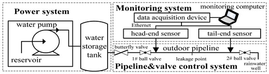
Figure 5.
Experimental platform schematic diagram.
To ensure the method’s adaptability to practical scenarios, the experiment included multiple leakage conditions and repeated measurements. 1. Leakage pressure: 0.3 MPa, 0.5 MPa, and 0.8 MPa (covering common urban pipeline pressures); 2. Leakage aperture: 0.3 mm, 0.5 mm, and 0.7 mm (simulating micro- to moderate leakage); 3. Leakage positions: three key points on the 36 m pipeline (near the head-end, middle, and near the tail-end) to consider propagation distance impacts; 4. Measurements: 10 repeats per “pressure–aperture–position” combination (5 for sudden leakage and 5 for steady leakage), with valid data retained after excluding interference-induced invalid tests.
The outdoor pipeline is welded from the DN80 galvanized seamless steel pipe (Shandong Iron and Steel Group Co., Ltd., Jinan, Shandong, China), with a total length of 36 m. The inlet of the outdoor pipeline is connected to the indoor pipeline system through a rubber hose. The outdoor pipeline site is shown in Figure 6. The head-end/tail-end sensors are shown in Figure 7, and the data acquisition device is shown in Figure 8.
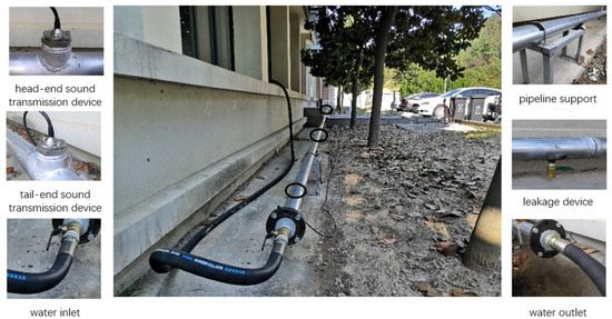
Figure 6.
Testing pipeline site.
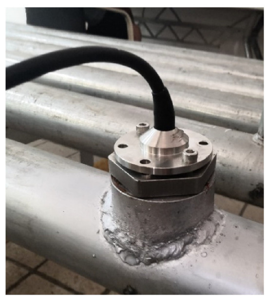
Figure 7.
Head-end/tail-end sensors.
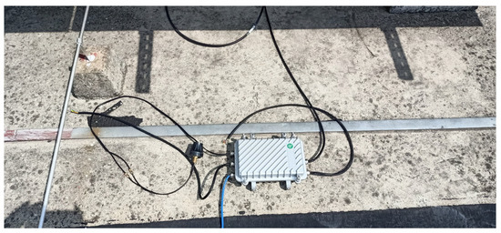
Figure 8.
Data acquisition device.
3.2. Analysis of Leakage Infrasound Signal
The leakage infrasound signal is obtained from the head-end and tail-end infrasound sensors shown in Figure 6, and there are four main sources of noise. (1) Pipe wall vibration noise: When the water pump is running, this noise is transmitted to the test pipeline through a connecting hose. (2) Power frequency interference: The system power supply is converted from a 220 V, 50 Hz AC signal to a 24 V DC signal, and there is 50 Hz power frequency interference in this process. (3) Environmental noise: Including outdoor traffic noise, construction noise, and other ambient disturbances. (4) Measurement and transmission errors: The measurement error of the sensors themselves and the error from the signal transmission process also exist.
For all valid tests, head-end and tail-end sensors synchronously collected signals (1000 Hz sampling rate). Targeted adjustments were made for special conditions: extended sampling for micro-leakage (to capture weak signals) and anti-vibration pads for high-pressure tests (to reduce vibration interference), ensuring signal authenticity.
To obtain a typical leakage signal waveform, when the pipeline pressure is 0.5 MPa, the leakage aperture is set to 0.5 mm, the ball valve at the leakage position is quickly opened and then closed, and the sensor signal at the head-end is subsequently obtained, as shown in Figure 9. The frequency spectrum of the signal obtained by the Fourier transform is shown in Figure 10.
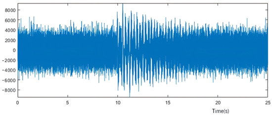
Figure 9.
Time-domain diagram of head-end sensor signal.
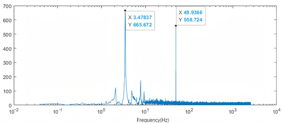
Figure 10.
Signal frequency domain diagram.
As shown in these figures, the time-domain signal of the head-end sensor is significantly affected by noise and is basically submerged by background noise. The leakage occurs after 10 s, with the signal reaching its maximum amplitude. At the beginning of leakage, the signal amplitude suddenly increases, making it an impulse signal. After the leakage starts, the signal becomes an oscillation signal, and this conforms to the characteristics of the leakage infrasound source.
4. Results and Discussion
- (1)
- Discussion of denoising results of simulation signals
Construct a 5 Hz sine wave as a pure signal, superimpose a 50 Hz power frequency signal and a white noise signal, and then use it as a test signal, as shown in Figure 11.
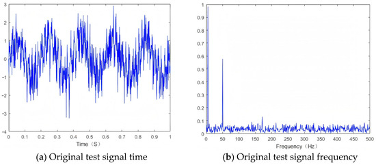
Figure 11.
Original test signal.
The rationale for selecting these two types of interference sources lies in the measured noise Power Spectral Density (PSD) characteristics at the pipeline experiment site. Background noise under the pipeline non-leakage condition was collected using an infrasound sensor, and its Power Spectral Density (PSD) was analyzed via the Welch method in MATLAB R2024a (MathWorks, Natick, MA, USA) with the Signal Processing Toolbox. All subsequent data processing (including wavelet decomposition, Fourier transform, and calculation of SNR/RMSE) was also completed in this software. The results show that the noise spectrum exhibits a significant power frequency peak at 50 Hz, and presents a flat distribution approximating white noise within the 10–500 Hz wide frequency range. This is fully consistent with the interference types added in the simulation, verifying the practical rationality of the simulation noise settings.
In order to avoid edge distortion during signal decomposition and reconstruction, the wavelet basis function is required to have good regularity and a small vanishing distance [31,32]. Therefore, wavelet basis functions such as symN, dbN, or coifN—with approximate symmetry, small vanishing moments, and regularity—can be selected. After conducting several tests on the influence of different wavelet basis functions on the SNR (signal-to-noise ratio) and RMSE (root mean square error), the db3 basis function is selected.
After determining the basis function, the reconstructed signals of different decomposition layers are analyzed using a fixed threshold. In order to quantitatively analyze the denoising effect, the SNR and RMSE methods are used to evaluate the results. The larger the SNR, the better the denoising effect; the smaller the RMSE, the more consistent the denoised signal is with the real signal. The formulae of SNR and RMSE are as follows.
In the formulae: —signal length, —original signal, and —denoised signal.
Using the db3 basis function, wavelet denoising is performed on the test signal. Table 1 shows the impact of different decomposition layers on the denoising results. It can be seen from the data in the table that, when the number of decomposition layers is five, the improved threshold function method has the best denoising effect, with the largest SNR of 19.5107 dB and the smallest RMSE of 0.07942.

Table 1.
Effect of different decomposition layers on noise reduction.
- (2)
- Discussion of denoising results of measured signals
Collect on-site measured infrasound leakage signals, select db3 as the wavelet basis function, and decompose the signals into five layers. Then, use the soft threshold method, the hard threshold method, and the improved threshold method to denoise and reconstruct the original signal. The original infrasound signal of the head-end sensor is shown in Figure 7, and the reconstructed time-domain and frequency-domain signals of the original signal are shown in Figure 12, Figure 13 and Figure 14.
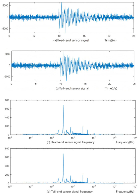
Figure 12.
Soft threshold method.
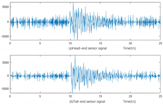
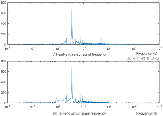
Figure 13.
Hard threshold method.
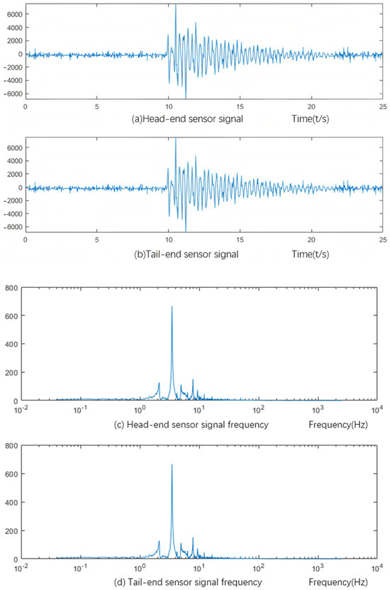
Figure 14.
New threshold method.
The improved method showed stable performance across 10 repeated tests for each condition (averaged results reported previously). Taking the 0.5 MPa, 0.5 mm case as an example, its SNR averaged 17.59 ± 0.31 dB (standard deviation, SD) and RMSE averaged 0.083 ± 0.005 (SD), with fluctuations <2%—far smaller than soft threshold (SNR: 12.43 ± 0.65 dB; RMSE: 0.142 ± 0.011) and hard threshold (SNR: 13.18 ± 0.52 dB; RMSE: 0.130 ± 0.008) methods. Even for micro-leakage (0.3 MPa and 0.3 mm), its SNR averaged 15.87 ± 0.44 dB and RMSE averaged 0.098 ± 0.007, confirming low variability and reliable performance. All reported SNR/RMSE values are averages of 10 repeated runs, with SDs provided to reflect data variability.
To quantitatively evaluate the denoising performance of the proposed method on real leakage data, we calculated the signal-to-noise ratio (SNR) and root mean square error (RMSE) for the measured infrasound signals—focusing on the 0.5 MPa pressure and 0.5 mm aperture condition—both before and after denoising, and compared the results with the soft and hard threshold methods. For the original measured signal (without denoising), the SNR was 8.26 dB and the RMSE was 0.215, indicating severe noise interference that submerged weak leakage features. After denoising with the soft threshold method, the SNR increased to 12.43 dB (an improvement of 5.16 dB) and the RMSE decreased to 0.142 (a reduction of 41.1%); the hard threshold method yielded an SNR of 13.18 dB (an improvement of 4.41 dB) and an RMSE of 0.130 (a reduction of 36.2%). In contrast, the improved threshold method achieved a significantly better performance: the SNR rose to 17.59 dB (an increase of 9.33 dB compared to the original signal) and the RMSE dropped to 0.083 (a reduction of 61.4% compared to the original signal). Importantly, this superior performance was not limited to the 0.5 MPa/0.5 mm condition—similar trends were observed in other measured scenarios, such as the 0.3 MPa pressure and 0.3 mm micro-leakage (where the improved method increased SNR by 8.72 dB and reduced RMSE by 58.3% relative to the original signal), and the 0.8 MPa pressure and 0.7 mm moderate leakage (where SNR improved by 10.15 dB and RMSE decreased by 63.7%). These results confirm that the proposed method effectively enhances signal quality for real infrasound leakage data, not just simulated signals.
It can be seen from the time-domain diagrams in Figure 12a, Figure 13a and Figure 14a that, after five-layer decomposition and denoising of the original infrasound leakage signal, the signal processed by the soft threshold method has the most burrs and the largest noise amplitude, while the improved threshold method is closer to the original infrasound leakage signal in terms of expressing signal details, and has the best effect. According to the frequency-domain diagrams in Figure 12b, Figure 13b and Figure 14b, it can be seen that the soft threshold and hard threshold methods leave more noise in the 10–100 Hz frequency band, and there is a 50 Hz power frequency interference signal; in contrast, the improved threshold method separates background noise more thoroughly. Based on the information in Table 1 and Figure 12, Figure 13 and Figure 14, it can be concluded that the improved threshold function method achieves the best denoising effect.
5. Conclusions
Aiming at the problem that pipeline leakage signals are greatly affected by background noise, a wavelet algorithm with an improved threshold function was proposed to realize ideal denoising of the original leakage signals.
(1) To solve the constant deviation and discontinuity problems of traditional soft and hard threshold functions, an improved threshold function denoising method for infrasound signals was established, and the continuity and convergence of the improved function’s properties were proved. This method is continuous and high-order differentiable; the shrinkage degree of the threshold function can be adjusted by changing the adjustment factor α, and thus it can be used to process different types of infrasound leakage signals.
(2) We completed multi-layer wavelet decomposition of typical infrasound leakage signals and reconstructed the original signals after wavelet denoising. By analyzing the time–frequency signals denoised with different methods, it can be concluded that the improved threshold method achieves the most ideal denoising effect and can effectively remove power frequency interference signals. The denoising results show that, compared with the soft threshold method and the hard threshold method, the SNR is increased by 5.1326 dB and 4.2148 dB, and the RMSE is reduced by 41.19% and 34.65%, respectively. This verifies the applicability and feasibility of the improved wavelet denoising method for denoising infrasound leakage signal data.
Future work will focus on three directions to further enhance the method’s practicality. First, optimizing the adjustment factor α with adaptive algorithms (e.g., reinforcement learning or Bayesian optimization) to enable the real-time self-tuning of the threshold function according to dynamic noise characteristics in complex pipeline environments. Second, integrating the improved wavelet method with deep learning models (e.g., CNN or Transformer) to handle non-stationary noise components that are currently challenging to separate, such as transient mechanical vibrations from pipeline joints. Third, validating the method in larger-scale field tests covering diverse pipeline materials (e.g., steel and plastic) and operating pressures so to assess its robustness across real-world scenarios and to lay a foundation for engineering applications.
Author Contributions
Conceptualization, Z.L.; methodology, Z.L.; software, J.T.; validation, B.L.; formal analysis, J.T.; investigation, J.T.; resources, Y.L.; data curation, B.L.; writing—original draft preparation, Z.L.; writing—review and editing, T J.; visualization, J.T.; supervision, F.Y.; project administration, Y.L.; funding acquisition, B.L. All authors have read and agreed to the published version of the manuscript.
Funding
This research was funded by the National Natural Science Foundation of China (Grant No. 52202508), the Open Project of Guangxi Key Laboratory of Automobile Components and Vehicle Technology in 2024 (Grant No. 2024GKLACVTKF02), the Central Government Guidance Fund Project for Local Science and Technology Development (Xinjiang Production and Construction Corps) (Grant No. 2024YD012), the Postdoctoral Innovation Project of Shandong Province (Grant No. SDCX-ZG-202400208), and Qingdao’s Key Technology Research and Industrialization Project (Grant No. 24-1-2-qljh-13-gx).
Data Availability Statement
The original contributions presented in this study are included in the article. Further inquiries can be directed to the corresponding author(s).
Acknowledgments
The authors are deeply grateful to Guangxi University of Science and Technology and Shandong Changlin Machinery Group Co., Ltd. for their support of this research.
Conflicts of Interest
Author Baogang Li was employed by the company Shandong Changlin Machinery Group Co., Ltd. The remaining authors declare that the research was conducted in the absence of any commercial or financial relationships that could be construed as a potential conflict of interest.
References
- Wan, J.L.; Deng, Y.L.; Li, Y. A review on detection and defect identification of drainage pipeline. Sci. Technol. Eng. 2020, 20, 13520–13528. [Google Scholar]
- Wang, H.C.; Li, Q.; Luo, Y. A similarity-based locating method of negative pressure wave caused by pipeline leakage. Oil Gas. Storage Transp. 2021, 40, 679–684. [Google Scholar]
- Zhou, Z.M.; Zhang, J.; Yang, K.L.; Zhang, L.L. Development and adaptability of gas transmission pipeline leak detection technology. Oil-Gas. Field Surf. Eng. 2019, 38, 6–12. [Google Scholar]
- Murvay, P.S.; Silea, I. A survey on gas leak detection and localization techniques. J. Loss Prev. Process Ind. 2012, 25, 966–973. [Google Scholar] [CrossRef]
- Hao, Y.M.; Yao, Q.; Jiang, J.C.; Xing, Z.X.; Xu, N. Simulation analysis of influence mechanism on infrasound propagation from urban pipeline leakage. Res. Explor. Lab. 2021, 40, 57–60, 82. [Google Scholar]
- Zhang, Q.; Zhao, P.; Wang, Y. Simulation and experimental study on infrasonic source of gas pipeline leakage. Autom. Instrum. 2023, 44, 116–120. [Google Scholar]
- Chilo, J.; Lindblad, T. Real-Time Signal Processing of Infrasound Data Using 1D Wavelet Transform on FPGA Device. In Proceedings of the 2007 15th IEEE-NPSS Real-Time Conference, Berkeley, CA, USA, 29 April–4 May 2007; pp. 1–6. [Google Scholar]
- Du, X.; Leng, X.; Rao, S.; Feng, L. Debris Flow Infrasound Denoising Based on Improved Wavelet Threshold Algorithm. In Proceedings of the 2022 IEEE International Conference Mechatron Autom, Guilin, China, 7–10 August 2022; pp. 1–6. [Google Scholar]
- Walker, D.; Hedlin, M.A.H. Wind-noise reduction for infrasonic measurements using adaptive line enhancement. J. Atmos. Ocean. Technol. 2010, 27, 1731–1742. [Google Scholar]
- Mallat, S.; Hwang, W.L. Singularity detection and processing with wavelets. In Proceedings of the IEEE International Conference on Acoustics, Speech, and Signal Processing, San Francisco, CA, USA, 23–26 March 1992; IEEE Press: Piscataway, NJ, USA, 1992; pp. 1–20. [Google Scholar] [CrossRef]
- Xu, Y.; Weaver, J.B.; Healy, D.M.J. Wavelet transform domain filters: A spatially selective noise filtration technique. IEEE Trans. Image Process 1994, 3, 747–758. [Google Scholar]
- Donoho, D.L.; Johnstone, J.M. Ideal spatial adaptation by wavelet shrinkage. Biometrika 1994, 81, 425–455. [Google Scholar] [CrossRef]
- Donoho, D.L. De-noising by soft-thresholding. IEEE Trans. Inf. Theory 1995, 41, 613–627. [Google Scholar] [CrossRef]
- Gao, H.; Bruce, A.G. Waveshrink with firm shrinkage. Stat. Sin. 1997, 7, 855–874. [Google Scholar]
- Luisier, F.; Blu, T.; Unser, M. A new SURE approach to image denoising: Interscale orthonormal wavelet thresholding. IEEE Trans. Image Process 2007, 16, 593–606. [Google Scholar] [CrossRef]
- Li, Q.Q.; Qin, B.Y.; Si, W.; Wang, R.Q.; Liu, B.; Ma, S.L.; Wang, X. Wavelet adaptive threshold estimation algorithm optimized by hybrid particle swarm and its application in partial discharge denoising. High. Volt. Eng. 2017, 43, 1485–1492. [Google Scholar]
- Wang, X.X.; Li, Y.Y.; Zhang, Z.Z. Improved wavelet threshold denoising algorithm for acoustic signals based on simulated annealing. Tech. Acoust. 2024, 43, 456–463. (In Chinese) [Google Scholar] [CrossRef]
- Liu, Y.Y.; Chen, K.K.; Zhao, W.W. Pipeline infrasound denoising via Beluga Whale Optimization-VMD combined with wavelet thresholding. Chin. J. Sci. Instrum. 2024, 45, 123–131. [Google Scholar]
- Hao, Y.M.; Yao, Q.; Zhu, Y.L.; Xing, Z.; Jing, J.; Xu, N.; Yang, J. Signal processing of infrasound leakage in urban pipelines based on spectral analysis. J. Pipeline Syst. Eng. Pr. 2023, 14, 04023007. [Google Scholar] [CrossRef]
- Sun, X.X.; Zhou, Y.Y. Pipeline Leakage Signal Processing Method Based on Improved Adaptive Optimal Kernel Time-Frequency Distribution. China Patent CN202410211234.7, 18 March 2024. (In Chinese). [Google Scholar]
- Peng, S.; Xing, J.; Liu, X. A rolling bearing vibration signal noise reduction processing algorithm using the fusion HPO-VMD and improved wavelet threshold. Symmetry 2025, 17, 1316. [Google Scholar] [CrossRef]
- Luan, J.; Liu, L.; Cui, B. Denoising of ceramic detection signals based on the combination of variational modal decomposition optimized by improved secretary bird optimization algorithm and wavelet thresholding. Rev. Sci. Instrum. 2025, 96, 015103. [Google Scholar] [CrossRef] [PubMed]
- Cheng, K.W.; Zhi, F.Z.; Bo, H.C.; Yong, Y. Denoise for propeller acoustic signals based on the improved wavelet thresholding algorithm of CEEMDAN. Cogent Eng. 2024, 11, 2327570. [Google Scholar] [CrossRef]
- Huang, Q.; Deng, Q.; Li, Z.; Luo, P. Application of a modified wavelet threshold denoising algorithm in system identification of WPTS. J. Power Electron. 2024, 24, 1150–1162. [Google Scholar] [CrossRef]
- Zhang, Y.; Ding, W.; Pan, Z.; Qin, J. Improved wavelet threshold for image de-noising. Front. Neurosci. 2019, 13, 39. [Google Scholar] [CrossRef] [PubMed]
- Zhu, G.; Liu, B.; Yang, P.; Fan, X. Image denoising method based on improved wavelet threshold algorithm. Multimed. Tools Appl. 2024, 83, 67997–68011. [Google Scholar] [CrossRef]
- Cui, H.M.; Zhao, R.M.; Hou, Y.L. Improved threshold denoising method based on wavelet transform. Phys. Procedia 2012, 33, 1354–1359. [Google Scholar] [CrossRef]
- Li, X.; Yao, H. Improved signal processing algorithm based on wavelet transform. J. Multimed. 2013, 8, 311–317. [Google Scholar] [CrossRef]
- Gao, X.J.; Gao, Z.G. Research on wavelet threshold denoising algorithm for images. Electron. Opt. Control 2007, 14, 148–151. (In Chinese) [Google Scholar] [CrossRef]
- Zhang, W.Q.; Song, G.X. Signal denoising in wavelet domain based on a new threshold function. J. Xidian Univ. 2004, 31, 296–303. (In Chinese) [Google Scholar] [CrossRef]
- Chen, P.; Zhang, Q. Classification of heart sounds using discrete time-frequency energy feature based on S transform and the wavelet threshold denoising. Biomed. Signal Process. Control. 2020, 57, 101684. [Google Scholar] [CrossRef]
- Ling, T.H.; Liu, H.R.; Zhang, L. Construction method of biorthogonal wavelet basis and its application in blasting vibration signal analysis. J. Vibr Shock. 2018, 37, 8–15. (In Chinese) [Google Scholar] [CrossRef]


Disclaimer/Publisher’s Note: The statements, opinions and data contained in all publications are solely those of the individual author(s) and contributor(s) and not of MDPI and/or the editor(s). MDPI and/or the editor(s) disclaim responsibility for any injury to people or property resulting from any ideas, methods, instructions or products referred to in the content. |
© 2025 by the authors. Licensee MDPI, Basel, Switzerland. This article is an open access article distributed under the terms and conditions of the Creative Commons Attribution (CC BY) license (https://creativecommons.org/licenses/by/4.0/).