Article

Predicting Real-Time Carbon Emissions for Power Grids Using Graph Convolutional Networks

1
State Grid Jibei Electric Power Company Ltd., Beijing 100054, China
2
State Grid Jibei Electric Power Company Limited Management Training Center, Beijing 102401, China
3
State Key Laboratory of Submarine Geoscience, Department of Automation, Shanghai Jiao Tong University, Shanghai 200240, China
*
Author to whom correspondence should be addressed.
Machines 2025, 13(11), 1061; https://doi.org/10.3390/machines13111061
Submission received: 8 October 2025 / Revised: 5 November 2025 / Accepted: 13 November 2025 / Published: 18 November 2025

Abstract

Accurate prediction of carbon emissions is crucial for both providing effective carbon reduction guidance to the power grid sector and driving society-wide carbon emission reduction. Existing methods based on power flow calculation theory heavily rely on real-time grid parameters and cannot accurately predict grid carbon emissions. To address the challenge, this paper proposes a novel spatiotemporal prediction model by integrating graph convolutional networks (GCNs) and temporal convolutional networks (TCNs). The GCN layer enhances node representation by aggregating neighborhood information, while the TCN layer captures long-term temporal dependencies through expanded causal convolutions. Experiments conducted on the IEEE 14-bus system demonstrate that the model achieves high accuracy and real-time processing capabilities, confirming its robustness and practical value for dynamic carbon emission predictions.

1. Introduction

The carbon emissions provide key guidance for developing new power systems, conducting precise carbon accounting, and evaluating the value of green electricity consumption [1,2,3,4]. Calculating regional dynamic carbon emissions is challenging because it involves modeling power flow tracking for electricity consumption across different time intervals within a region. Due to the multi-voltage-level feature in power grids, the power flow at each level undergoes dynamic changes. Consequently, constructing an accurate and efficient model is important yet complex [5,6,7].
Prediction methods for the carbon emissions generally fall into three major categories: scenario prediction models, linear regression models, and machine learning models [8]. The long-range energy alternatives planning system (LEAP) is a scenario prediction model that can be used to predict carbon emissions from power grids when combined with scenario analysis. Wang and Watson [9] developed four scenario pathways under a cumulative carbon budget to explore China’s low-carbon transition in power, transport, industry, and household sectors. Furthermore, the LEAP model is applied to construct and compare four exploratory scenarios for Panama’s electricity sector, quantifying the trade-offs between system costs, global warming potential, and resource diversity under different renewable energy deployment pathways through 2026 [10]. The core advantage of linear regression models is their exceptional interpretability, which enables the clear quantification of the relationship between power generation and total carbon emissions. This provides a direct and transparent basis for energy dispatch decisions. Furthermore, the model is computationally efficient and easy to implement, enabling the rapid establishment of predictive benchmarks [11,12]. A hyperbolic tangent function-based linear regression model [13] is proposed to capture seasonal and diurnal trends in electricity consumption for short-term forecasting and carbon emission estimation. Ref. [14] improves the existing stirpat model by incorporating carbon emissions into the modelling analysis. It uses ridge regression to address biased estimates in historical data and establishes a carbon emission prediction model for Shanghai’s electricity and energy sectors based on elasticity relationships.
Machine learning methods have been widely applied in the field of carbon emissions predictions and have demonstrated excellent performance in recent years. Ref. [15] proposes a CNN-LSTM-attention model combined with Bayesian optimization for precise prediction of carbon dioxide emissions from coal-fired power plants. Machine learning methods combining feature selection, linear regression, and the auto-regressive integrated moving average model (ARIMA) [16] can be employed to forecast short-term carbon emission intensity in power grids, providing precise predictive support for low-carbon dispatch. Furthermore, advanced deep learning architectures, including long short-term memory (LSTM) networks [17], support vector machine (SVM) [18], and TCN [19] offer viable approaches for predicting carbon emissions. These methods are capable of automatically capturing complex nonlinear dependencies and temporal patterns from large-scale historical operational datasets, thereby facilitating accurate and reliable forecasting of carbon emissions in electric power systems. Current research on carbon emissions prediction is increasingly focusing on the integration of multi-modal data, hybrid modeling approaches, and real-time adaptive learning techniques to enhance the accuracy of predictions across complex and dynamic power systems.
Inspired by [20], which shows that graph neural networks (GNNs) can be employed for spatio-temporal forecasting modeling, this paper proposes a novel carbon emissions prediction model based on GNNs for power grid systems. The proposed method leverages GNNs combined with advanced spatio-temporal feature extraction, which enables dynamic and accurate prediction of carbon emissions in power grid systems. The contributions of the study are summarized as follows:
  • Complex spatiotemporal data in power grid systems are structured into graph data, leveraging the powerful relational reasoning capabilities of graph neural networks to capture dynamic interactions between regional nodes.
  • The TCNs layer captures complex time-dependent relationships, enabling highly accurate predictions of power grid carbon emissions.
The remainder of this paper is organized as follows. The preliminaries and problem formulation is provided in Section 2, and the proposed carbon emissions prediction method is presented in Section 3. Then, the experimental results are given in Section 4. Section 5 concludes this study.

2. Preliminaries and Problem Formulation

2.1. A Carbon Calculation Model for Power Grid Nodes

The operation process of the power grid is shown in Figure 1. The power grid system first converts various energy sources including fuel, wind power, and hydropower into electricity through gas turbines, wind turbines, and hydroelectric stations. Subsequently, the generated electricity is transmitted via a unified grid network and intelligently dispatched and distributed by an energy management system to ensure real-time balance between power supply and demand. Stable electrical current is precisely delivered to diverse end-use terminals such as industrial zones and charging stations, effectively meeting the energy requirements for urban operations and development. Ultimately, this modern grid—integrating generation, transmission, distribution, and consumption—forms a highly efficient, reliable, and secure closed-loop energy supply system.
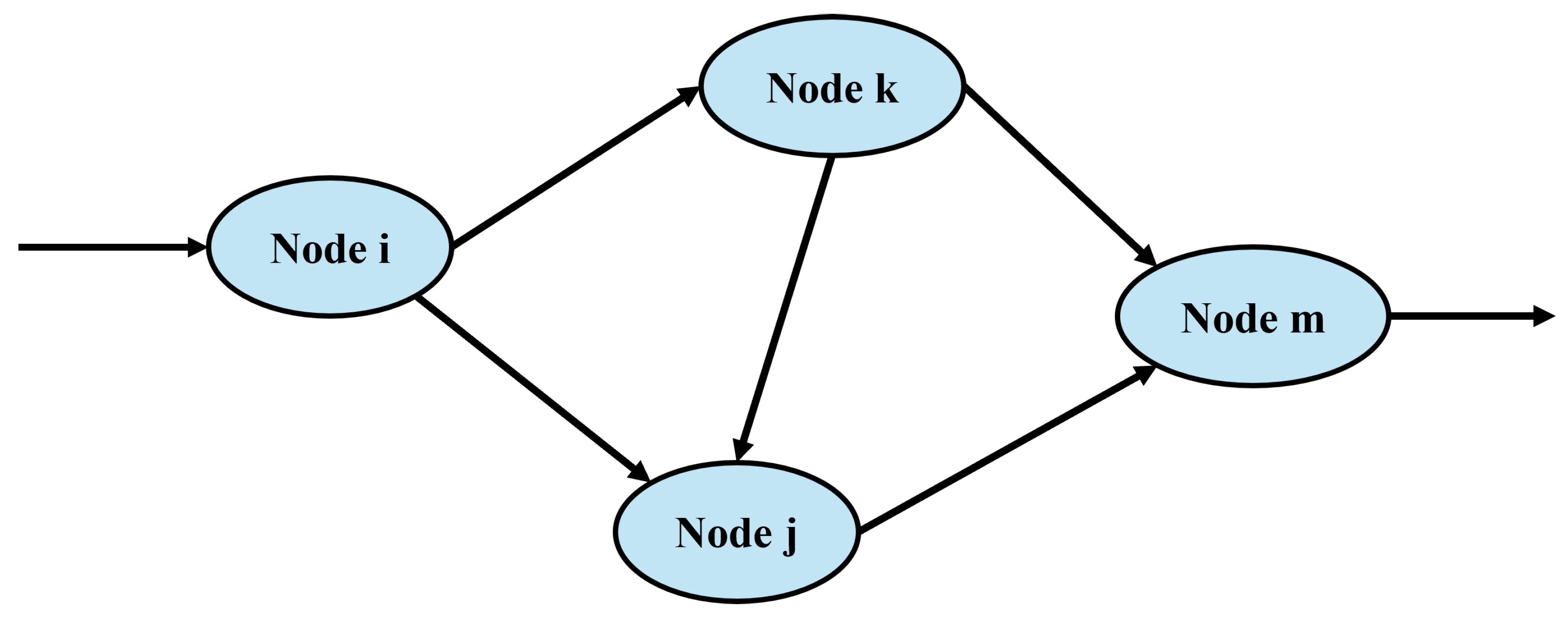
Carbon emission flows are modeled as virtual network flows coupled with the active power flow in the power grid, representing the carbon emissions associated with power transmission through branch circuits. A power grid system can be abstracted into the model shown in Figure 2:
Nodes i, j, k, and m represent entities such as substations, power plants, users, and so on. Typically, these nodes are used for consuming electricity, generating electricity, or voltage transformation. Each node satisfies the power balance and carbon emission balance equations as follows:
S k = i = 1 n S i k = j = 1 m S k j + S E k = i = 1 n E i k = j = 1 m E k j + E S
where S k represents the total electricity consumption of node k, S i k denotes the electricity supplied from node i, S k j indicates the electricity flowing to node j, S represents electricity consumed internally at node k. E k represents the total carbon emissions of node k, E i k denotes the carbon emissions originating from node i, E k j denotes the carbon emissions flowing to node j, E S denotes the carbon emissions generated by internal consumption of node k. n and m represent the number of incoming and outgoing nodes respectively. Formula (1) represents the balance equations for electricity and carbon flows in power grids and serves as a key basis for predicting grid carbon emissions.

2.2. Problem Description

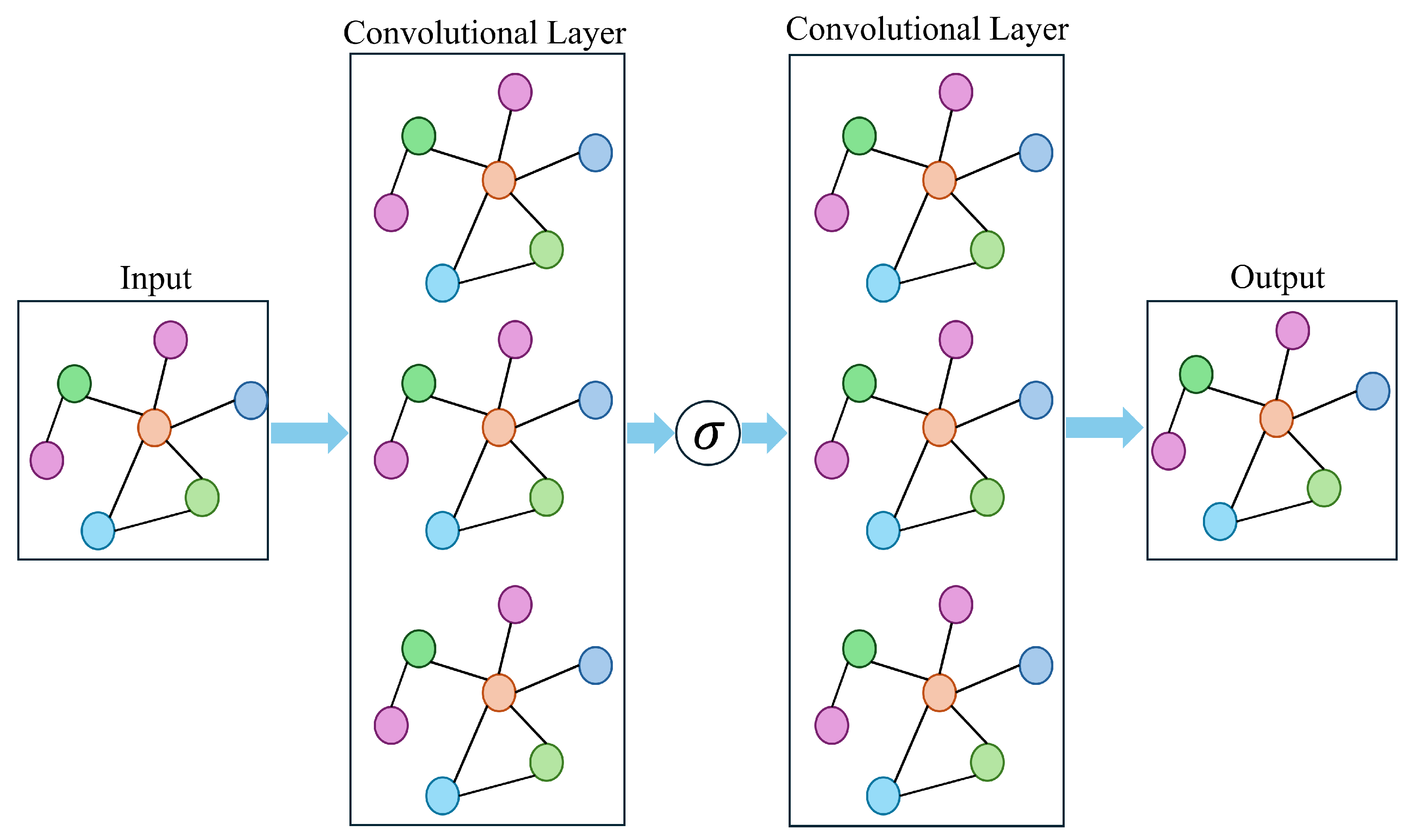
GCNs enable hierarchical feature extraction directly from graph-structured data through efficient convolutional operations, significantly enhancing performance in classification and prediction tasks while maintaining high computational efficiency [21,22]. The specific architecture is illustrated in Figure 3.
Consider a graph G = ( V , E ) with N = | V | vertices. To include self-loops, the modified adjacency matrix can be defined as follows:
A ^ = A + I N , D ^ i i = j A ^ i j , A ˜ = D ^ 1 / 2 A ^ D ^ 1 / 2
where D ^ is the degree matrix of A ^ , A ˜ is the symmetrically normalized adjacency matrix, adjacency matrix A R N × N .
In this work, the adjacency matrix A is defined as a binary matrix, where A i j = 1 if there is a direct transmission connection between node i and node j, and A i j = 0 otherwise. This binary representation captures the topological connectivity of the power grid without incorporating physical line parameters such as impedance or capacity, as the primary focus is on modeling spatial dependencies between regions. The graph structure is based on the IEEE 14-node system mentioned later, where nodes represent buses and edges represent transmission lines.
Given the node feature matrix X R N × F , the propagation rule of a GCN layer is defined as:
H ( l + 1 ) = σ A ˜ H ( l ) W ( l ) + 1 ( b ( l ) )
where H ( l ) R N × F ( l ) denote the node representations at the l-th layer, with H ( 0 ) = X , W ( l ) R F ( l ) × F ( l + 1 ) is a trainable weight matrix, b ( l ) R F ( l + 1 ) is a bias vector, σ ( · ) is a nonlinear activation function, and 1 is an all-ones column vector used to broadcast the bias.
In an element-wise form, the update rule for node i is expressed as:
h i ( l + 1 ) = σ j N ( i ) { i } A ˜ i j h j ( l ) W ( l ) + b ( l )
where N ( i ) denotes the set of neighbors of node i. This formulation allows each node to aggregate feature information from its neighborhood and transform it through learnable parameters.
For node-level tasks, the final node embeddings H ( L ) are directly used for downstream predictions. For graph-level tasks, a permutation-invariant readout function is applied to obtain a global representation:
z G = α H ( L )
where α can be implemented as sum-pooling, mean-pooling, or max-pooling over the node embeddings.
The computational complexity of a GCN layer is presented as follows:
O ( | E | F ( l ) + N F ( l ) F ( l + 1 ) )
where | E | is the number of edges, N the number of nodes, and F ( l ) , F ( l + 1 ) the input and output feature dimensions, respectively. The first term arises from sparse matrix multiplication with A ˜ , while the second corresponds to dense linear transformation.
Given a power grid system has M regions, each region contains both power generation and consumption facilities in a power grid system. The entire multi-region power grid system is modeled as a graph structure:
G t = ( V , E )
where Each node V represents a power grid region, edges E represent transmission connections between regions. Each node has a set of feature vectors x t . The data of each node are aggregated into the feature matrix X:
X = x 1 T x 2 T x N T T
The ultimate goal is to predict the carbon emissions Y t of each node at time step t by constructing GCNs.
Y t = G t ( X )
Based on the above discussion and analysis, in order to achieve effective prediction of grid carbon emissions, the following issues must be addressed.
  • Establish an accurate measurement model based on graph convolution networks for power grid systems.
  • Transform the output of the network topology matrices into a predictive form for carbon emissions.
  • Train the entire network to minimize prediction errors for the carbon emissions.

3. GCN-Based Carbon Emissions Prediction

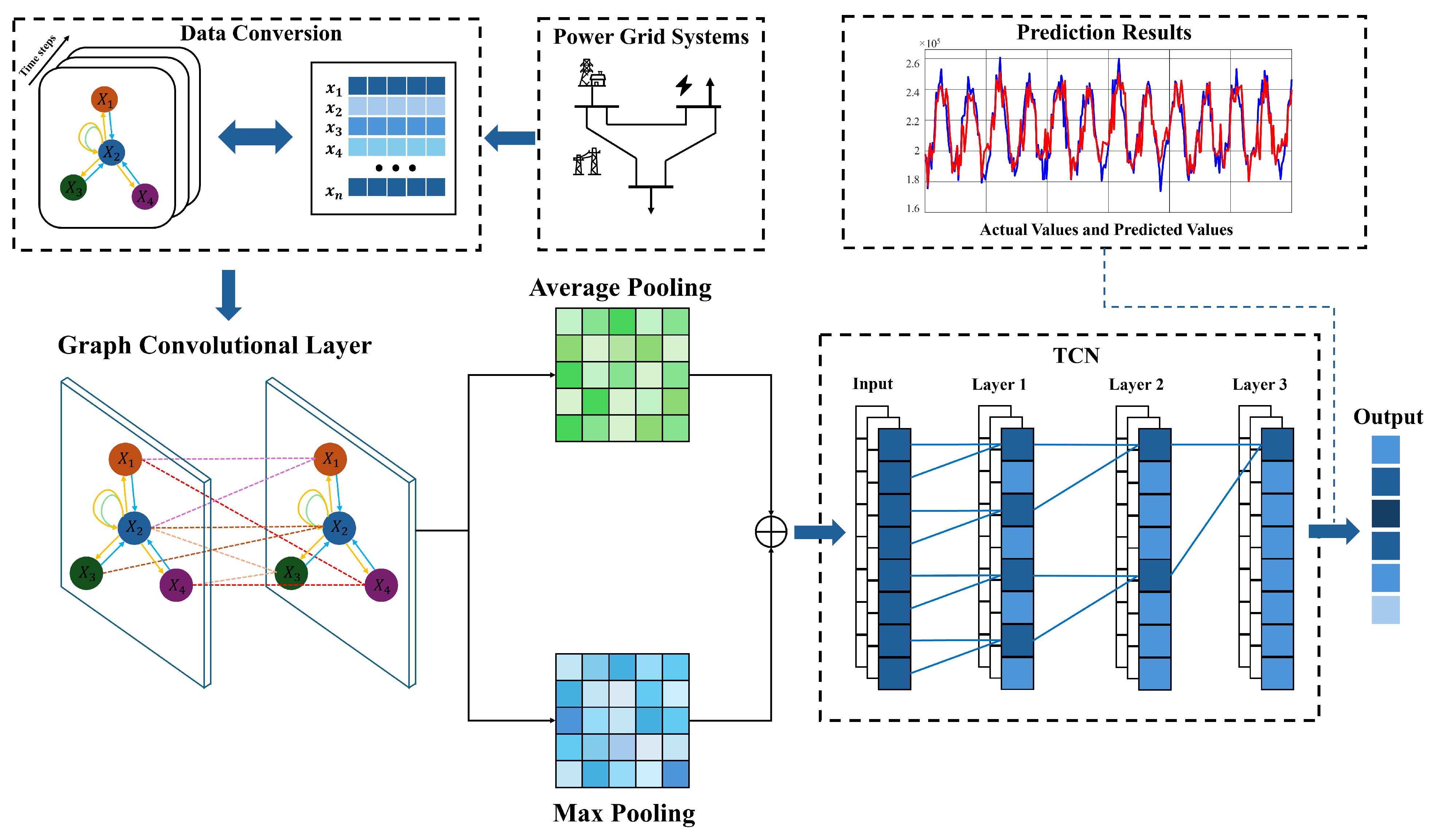
Figure 4 shows the architecture of the proposed GCN-based approach for predicting the carbon emissions, comprising three components: a graph convolutional layer, a pooling layer and a TCN layer. This section first introduces the architecture of the graph convolutional layer, then covers the pooling layer and the TCN layer, and finally presents the training method and objective function.

3.1. Graph Convolutional Layer

The propagation rules for each convolutional layer have been provided in Equation (3). Node regression output can be computed as:
y ^ i = w T h i ( L ) + b
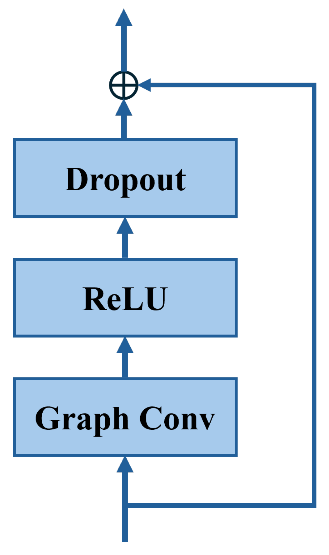
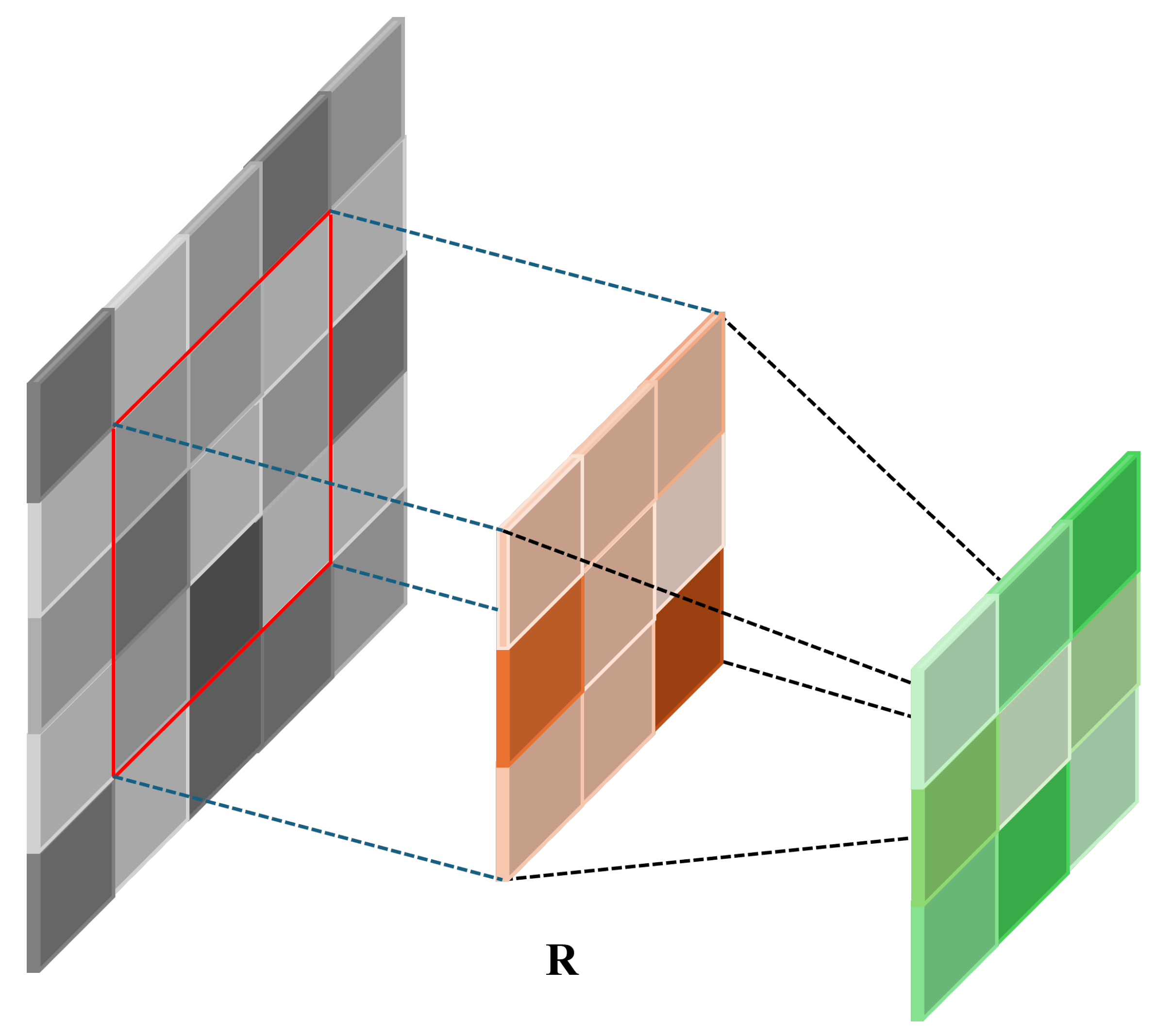
where h i ( L ) is the feature representation of the node at the final layer. Power networks exhibit distinct graph-structured characteristics, where each region can be regarded as a node in the graph, and power exchanges between regions form the edges [23,24]. The GCN layer effectively captures the mutual influence between regions by aggregating information from nodes and their neighboring nodes. Figure 5 illustrates the structure of a GCN layer.
Each regional node possesses multiple attributes. The GCN layer integrates these attributes with graph structural information to generate context-rich node embeddings. These embeddings not only reflect the node’s intrinsic states but also incorporate insights from its local graph structure, thereby providing a more comprehensive representation of the system operational status. The introduction of the GCN layer addresses the spatial limitations of purely temporal models. By incorporating graph structure information from each time step into node representations, the model can consider the real-time status of other regions while predicting carbon emissions at the current time step, leading to more accurate predictions.
The pooling layer is used to reduce the dimensionality of node features and graph structures while preserving important information. This is particularly useful for graph-level regression tasks, where a fixed-size representation of the entire graph is required. The operation of the pooling layer is shown in Figure 6. After passing through the graph convolutional layer, H ( l ) R N × d denotes the resulting node feature matrix. A mean pooling operation aggregates node features into a graph-level representation h g :
h G m e a n = MeanPool H ( l ) = 1 N i = 1 N h i ( l ) .
Max pooling operations can be computed as:
h G m a x = MaxPool H ( l ) = max i V h i ( l )
where h G m e a n , h G m a x R d . To construct a more informative and robust graph-level representation, this representation incorporates both average node information reflecting the system’s overall carbon emission baseline and extreme information from key nodes that may dominate total carbon emissions. Therefore, the pooling layer must perform both mean pooling and max pooling simultaneously, enabling the fully connected layer to make more accurate and reliable predictions. Feature concatenation between mean pooling and max pooling is performed as follows:
h G = h G m e a n h G m a x
where ‖ denotes the vector concatenation operation, h G R 2 d .
Since the pooling layer representation h G ( t ) consists of independent vectors and TCNs require sequence inputs of fixed time length, data transformation is necessary. This involves reconstructing h G ( t ) into a sliding window format, enabling the model to preserve temporal dependencies while allowing TCNs to effectively capture dynamic patterns across images.
Given a temporal window length L, the input for the k-th sample is constructed as:
X k = h G ( k L + 1 ) , h G ( k L + 2 ) , , h G ( k ) T
where X ( k ) R L × 2 d represents the sequence of pooling representations from the past L time steps. For k < L , zero-padding is applied:
X k = [ 0 , , 0 L k , h G ( 1 ) , , h G ( k ) ] T .
To match the input format of the TCN, the feature matrix is transposed as:
X k TCN = X k T R 2 d × L ,
where the final TCN input tensor X TCN R B × 2 d × L , B denotes the batch size, 2 d is the number of input channels, and L is the temporal length.
This construction establishes the mapping from the pooling output h G to the TCN input X TCN , enabling the model to capture the temporal dynamics of graph-level representations.

3.2. Temporal Convolutional Layers

Graph pooling operations generate compact representations of the system at each time step, which capture the global carbon emission characteristics of the grid. However, these representations evolve dynamically as the system undergoes changes in load, generation structure, and inter-regional power flows. To model these sequential dependencies, a TCN is introduced after the pooling operations. The TCN architecture is particularly suitable for predicting carbon emissions because it combines two essential properties [25,26,27,28]:
  • causal convolutions that strictly preserve temporal order and avoid information leakage from future to past.
  • dilated convolutions that increase the receptive field and enable long-term dependency modeling.
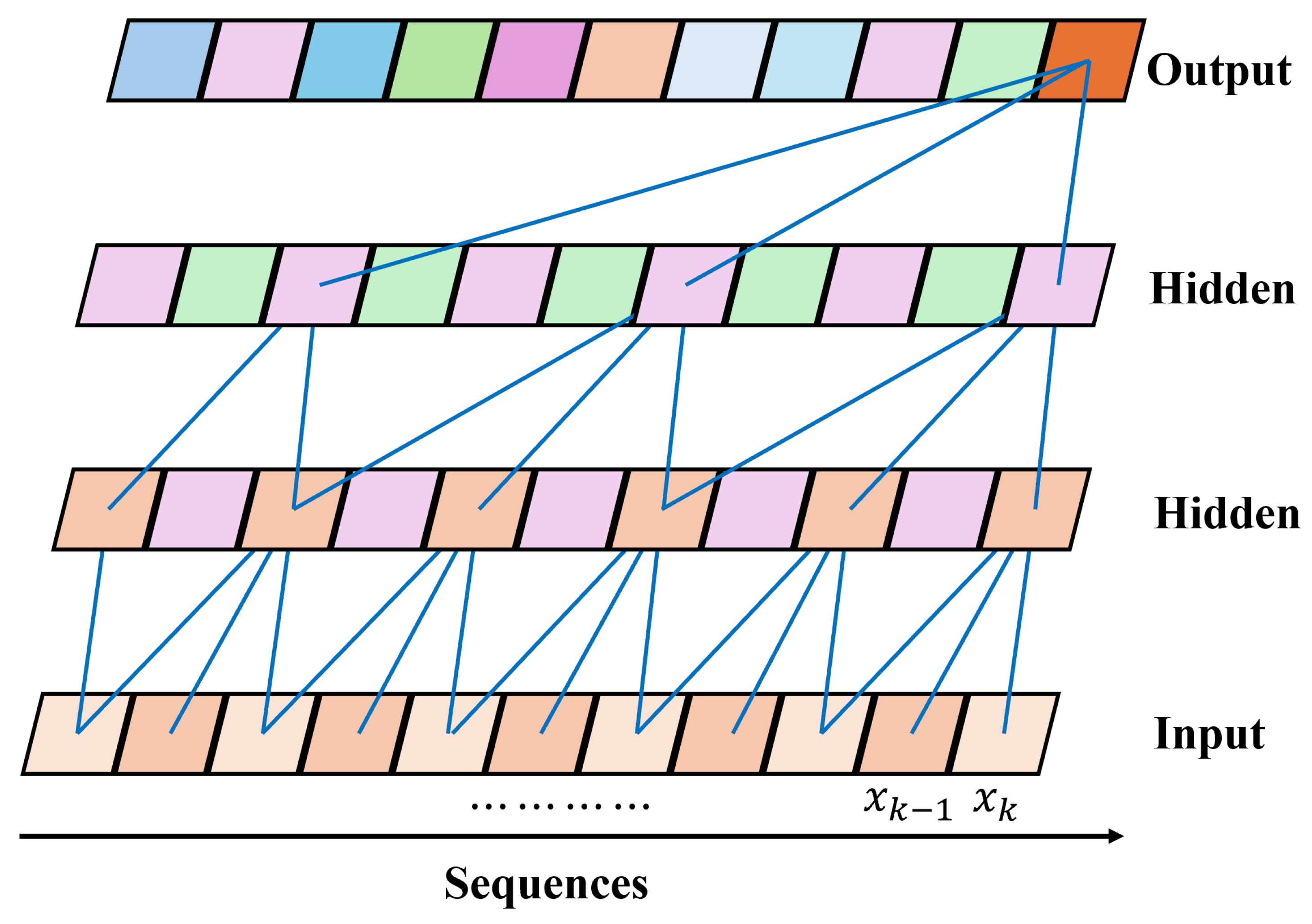
A dilated causal convolution is illustrated as shown in Figure 7. Given a temporal input sequence X TCN , an l-th layer dilated causal convolution can be expressed as follows:
( Z ( l ) ) c , t = c = 1 2 d i = 0 k 1 W c , c , i ( l ) X c , t m · i + b c ( l )
where k represents the kernel size, m represents the dilation factor, c denotes the output channel, and t denotes the time step. W and b denote weights and biases. X c , τ = 0 if τ < 0 , ensuring causality. This operation allows the model to capture both short-term and long-term dependencies by adjusting d across layers. Compared to recurrent networks, dilated convolutions can process sequences in parallel across time, significantly reducing training time while retaining the ability to model long-range dependencies.
Zero padding results in the output sequence containing extra padding elements at the end, which must be removed. To ensure that the output has the same length as the input, the convolution uses padding p = ( k 1 ) m and a cropping operator is applied:
Chomp p ( Z ) [ : , : , t ] = Z [ : , : , t ] , t = 0 , , L 1 .
This step removes the extra padded elements and guarantees that the convolution is strictly causal.
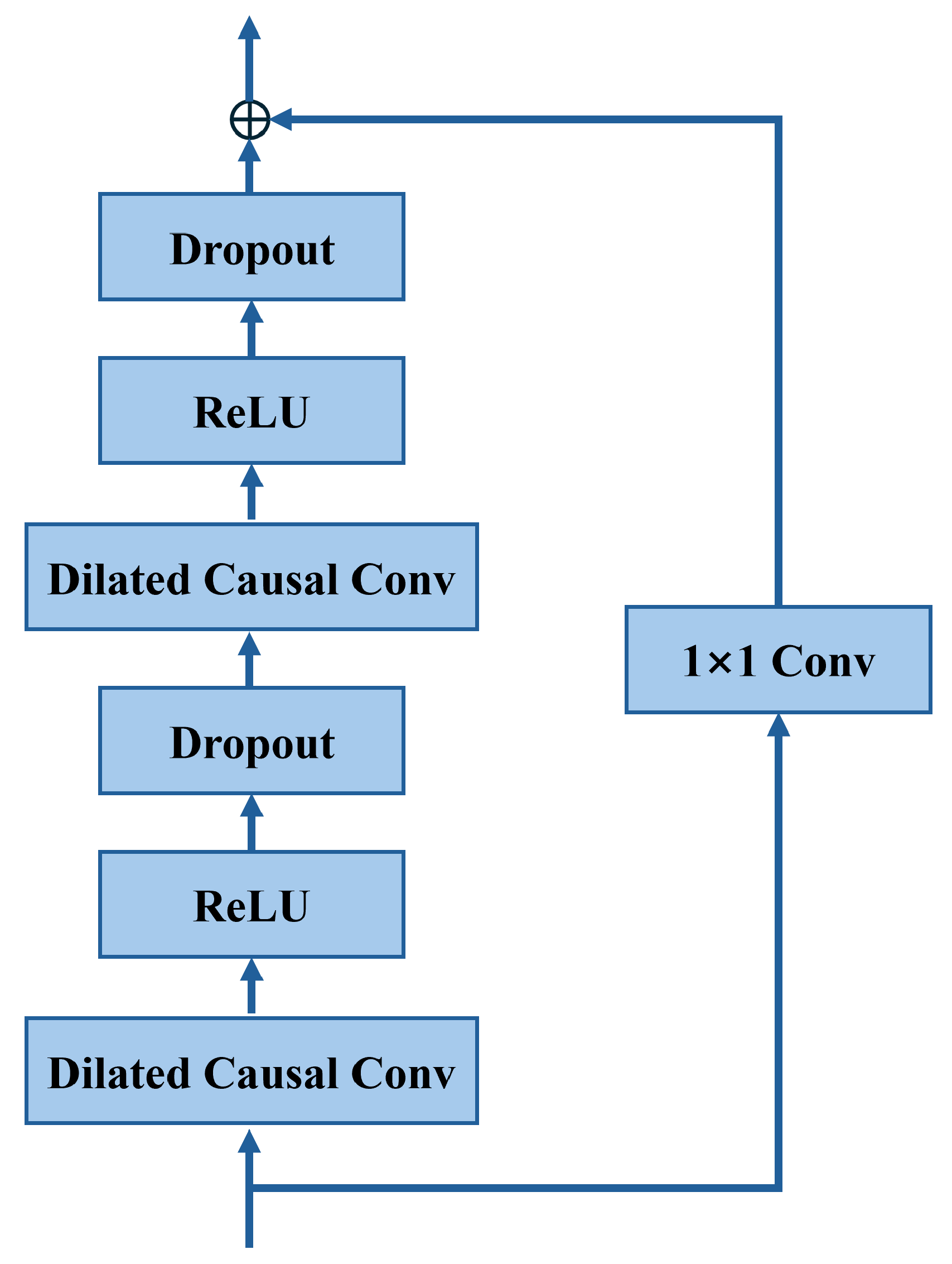
Therefore, each TCN architecture requires stacking two dilated causal convolutions, each followed by a ReLU activation function and a dropout operation with probability ρ . The residual connection is formulated as:
Y = ReLU R ( X ) + F ( X )
where F ( · ) denotes stacked dilated convolution, R ( · ) represents 1 × 1 convolution. Residual connections stabilize the optimization process, enabling effective training of deeper temporal convolutional neural networks. The structure of the final TCN block is shown in Figure 8.
Multiple temporal blocks are stacked with exponentially increasing dilation factors d = 2 ( = 0 , , N 1 ). The output of the stacked TCN is as follows:
Y ^ = T N 1 T 1 ( T 0 ( X ) )
where T ( · ) represents temporal block operations, the effective receptive field of the stacked TCN is as follows:
Q = 1 + ( k 1 ) = 0 L 1 d = 1 + ( k 1 ) ( 2 L 1 ) .
Note that Q quantifies the number of past steps that can be integrated into each output. This characteristic is crucial for predicting carbon emissions, as carbon emissions depend not only on instantaneous power generation and consumption but also on patterns formed through accumulation over hours or days.
The complexity of a single TCN layer is O L · k · 2 d · C out . Unlike RNN-based models whose complexity grows with sequential steps due to recursive dependencies, TCN layers allow parallel computation across all time steps, enabling efficient training on large-scale datasets.
Recurrent neural network architectures excel at time series modeling, but suffer from gradient vanishing issues, resulting in high training costs and difficulty capturing ultra-long dependencies. Transformer models, while powerful, require quadratic attention complexity O ( T 2 ) , making them less suitable for long-sequence power data. In contrast, Time Convolutional Networks (TCNs) achieve an ideal balance by integrating parallel processing, long-range dependency modeling, and computational efficiency. These advantages make TCNs particularly well-suited for predicting real-time regional carbon emissions—a domain where both timeliness and accuracy are critical.
The activation and layer-dimension settings were selected based on best practices reported in recent spatio-temporal forecasting literature [25,26,27,28]. ReLU activation provides stable gradient propagation, while three GCN layers and two TCN blocks yield sufficient receptive-field coverage for the IEEE 14-bus topology without over-parameterization. This configuration has proven effective in prior power-system applications [25,26].
Overall, the introduction of the TCN layer significantly enhances the model’s ability to track the evolutionary patterns of carbon emissions in power systems. By combining causal convolutions with dilated convolutions and residual learning, this framework achieves high predictive accuracy, robustness against non-stationary fluctuations, and scalability for long-term sequence data. This design ensures effective real-time carbon emissions prediction in actual grid operations.

3.3. Training Method

The training of the proposed GCN-based hybrid model is formulated as an optimization problem aimed at minimizing the discrepancy between predicted and actual carbon emission values. The overall objective function is defined as the mean squared error (MSE) between the ground truth carbon emissions Y and the model predictions Y ^ :
L ( Θ ) = 1 N i = 1 N ( y i y ^ i ) 2
where N denotes the number of samples in the training set, y i is the actual carbon emission value of the i-th sample, y ^ i is the corresponding predicted value, and θ represents the set of all trainable parameters in the model.
To prevent overfitting and enhance generalization capabilities, L 2 weight regularization is incorporated into the loss function. The regularized loss function is defined as follows:
L reg ( Θ ) = L ( Θ ) + λ Θ 2 2 ,
where λ is the regularization hyperparameter controlling the strength of penalty imposed on large weights.
The model parameters are updated iteratively using the Adam optimizer, which combines the advantages of AdaGrad and RMSProp. The update rules for the first and second moment estimates are as follows:
m t = β 1 m t 1 + ( 1 β 1 ) Θ L reg ( Θ t ) ,
v t = β 2 v t 1 + ( 1 β 2 ) [ Θ L reg ( Θ t ) ] 2
where m t and v t are estimates of the first moment and the second moment of the gradients, respectively, and β 1 , β 2 [ 0 , 1 ) are exponential decay rates. The parameters are then updated according to:
Θ t + 1 = Θ t η m ^ t v ^ t + ϵ
where m ^ t = m t / ( 1 β 1 t ) and v ^ t = v t / ( 1 β 2 t ) are bias-corrected moment estimates, η is the learning rate, and ϵ is a small constant added for numerical stability.
To further improve training efficiency and avoid overfitting, we employ a learning rate scheduler that reduces the learning rate when the validation loss plateaus. The update rule is defined as:
η t + 1 = η t · γ · I ( L val ( t ) > L val ( t 1 ) )
where γ is the decay factor, L val is the validation loss, and I ( · ) is the indicator function. Gradient backpropagation is performed through both temporal and graph convolutional layers. The gradient with respect to the weights of the GCN layer is computed as:
L W ( l ) = A ˜ T L H ( l + 1 ) · σ ( Z ( l ) ) · ( H ( l ) ) T
where Z ( l ) = A ˜ H ( l ) W ( l ) , σ denotes the derivative of the activation function, and A ˜ is the normalized adjacency matrix.
An early stopping strategy is adopted to terminate training when the validation loss does not improve for a predefined number of epochs. This ensures the model does not overfit while maintaining computational efficiency. The entire training process is summarized in Algorithm 1. This comprehensive training strategy ensures stable convergence, effective generalization, and high predictive accuracy for the proposed spatio-temporal model.
Algorithm 1 Training Procedure for GCN-based Model
Require: Training data D train , validation data D val
Ensure: Trained model parameters Θ
  1:
 Initialize parameters Θ
  2:
 while not converged do
  3:
    Sample a mini-batch from D train
  4:
    Forward pass to compute Y ^
  5:
    Compute loss L reg ( Θ ) using Equation (23)
  6:
    Backpropagate gradients
  7:
    Update parameters using Adam optimizer Equation (26)
  8:
    Compute validation loss L val
  9:
    if  L val does not improve for K epochs then
10:
      Break
11:
    end if
12:
    Update learning rate using Equation (27)
13:
 end while
The following experiments will validate the effectiveness of the proposed GCN-based approach for predicting carbon emissions.

4. Experimental Studies on GCN-Based Approach

4.1. IEEE 14-Bus Systems Verification

The IEEE 14-bus system is a widely used standard test network in power system analysis. It consists of 14 buses, 5 generators, 11 loads, and 20 transmission lines, operating at voltage levels of 60–132 kV with a total installed capacity of approximately 1.1 GW. Despite its compact structure, the system incorporates diverse topological features including radial and loop configurations. This design captures the heavy load characteristics of urban distribution networks while preserving voltage-reactive power coupling phenomena at transmission levels.
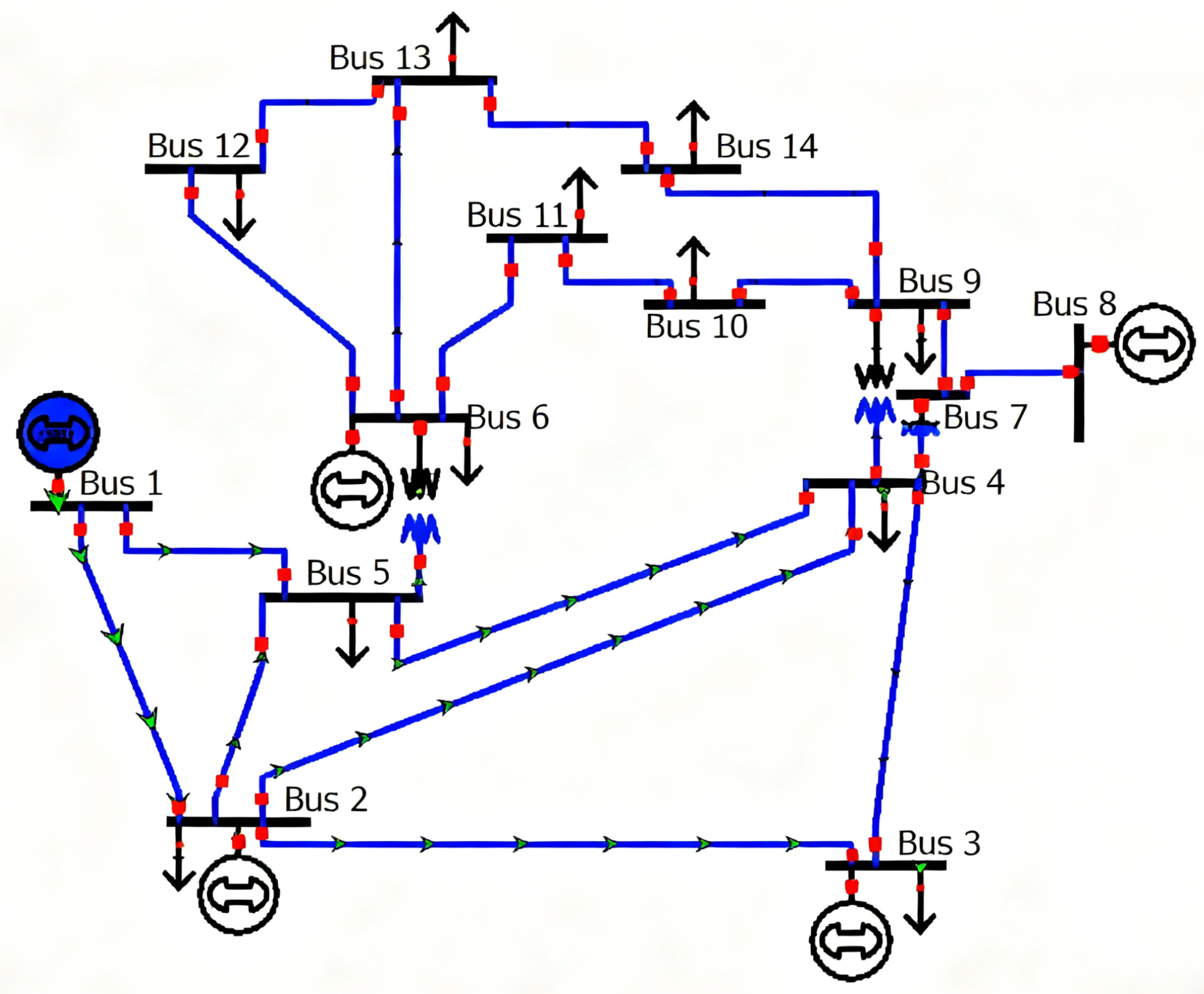
Despite its scaled-down size, the IEEE 14-bus system fully preserves transmission-distribution coupling, multi-voltage levels, and the multi-source-grid-load structure. It flexibly maps the spatiotemporal distribution of fossil units, renewable energy sources, and loads. Its publicly available and validated topology and unit carbon emissions data provide a standardized, reproducible testing environment for constructing “node-branch” carbon flow tracking, dynamiccarbon emissions, and carbon emission trend prediction models [29]. The overall structure of the IEEE 14-bus electric power system is shown in Figure 9.
Each node in the system is characterized by a feature vector containing six attributes: active power load ( P d ), reactive power load ( Q d ), active power generation ( P g ), reactive power generation ( Q g ), voltage magnitude (V), and voltage angle ( θ ). The target variable is the total carbon emission ( C e ) of the system at each time step, calculated as the sum of emissions from all generating nodes. Emissions are computed based on generator type and vary with load factor and time of day. At each time step t, each node input x t contains the following data features:
x t = P d T Q d T P g T Q g T V T θ T T
where x t R F . The input feature matrix X R N × F and the output Y R are normalized using StandardScaler before training.
The dynamic load and generation profiles were obtained from the open-source IEEE 14-bus benchmark dataset. Time-series variations were created by sampling 2000 steps from load-generation profiles in the MATPOWER simulation environment under random perturbations of ±5 % to emulate daily fluctuations. Carbon-emission values at each time step were computed using generator-specific emission coefficients published by Ma et al. [7] and Luo et al. [12].
Remark 1. 
To prevent data leakage and ensure a fair evaluation, the StandardScaler was fit only on the training set to compute the mean and standard deviation of each feature. The same scaling parameters were then applied to transform the validation and test sets, ensuring that no information from these sets influenced the normalization process.
The GCN-based model consists of three GCN layers with hidden dimension 128, followed by a temporal convolutional network with channel sizes [64, 32]. The sequence length for TCN is set to 10 time steps. The model is trained using the Adam optimizer with a learning rate of 0.001 and early stopping based on validation loss. During the training phase, data is fed into the model, and Algorithm 1 is executed to produce the trained model. The simulation consists of 2000 time steps, with the final 300 used as the test set. The average power generation of each generation node is shown in Table 1. The system’s total average power generation is 276.06 MW, and the total average load is 257.99 MW, indicating the system operates within a reasonable power balance range.
During the training phase, the loss function values for both the training and validation sets decrease as the number of training iterations increases. In the testing phase, the model’s output values closely approximate the true values. To quantitatively evaluate the predictive accuracy of the proposed model, the following commonly used metrics are employed:
RMSE = 1 N i = 1 N ( y i y ^ i ) 2 , R 2 = 1 i = 1 N ( y i y ^ i ) 2 i = 1 N ( y i y ¯ ) 2 , MAE = 1 N i = 1 N y i y ^ i
where y is the actual value, y ^ is the predicted value, y ¯ is the mean of the actual values.
It should be noted that, although the model is designed for node-level carbon emission prediction, the evaluation in this specific case study is performed at the system level by aggregating the predicted emissions of all nodes into a total value. This system-level total is used to compute the performance metrics: RMSE, MAE, and R 2 —enabling a straightforward and consistent comparison with baseline models.
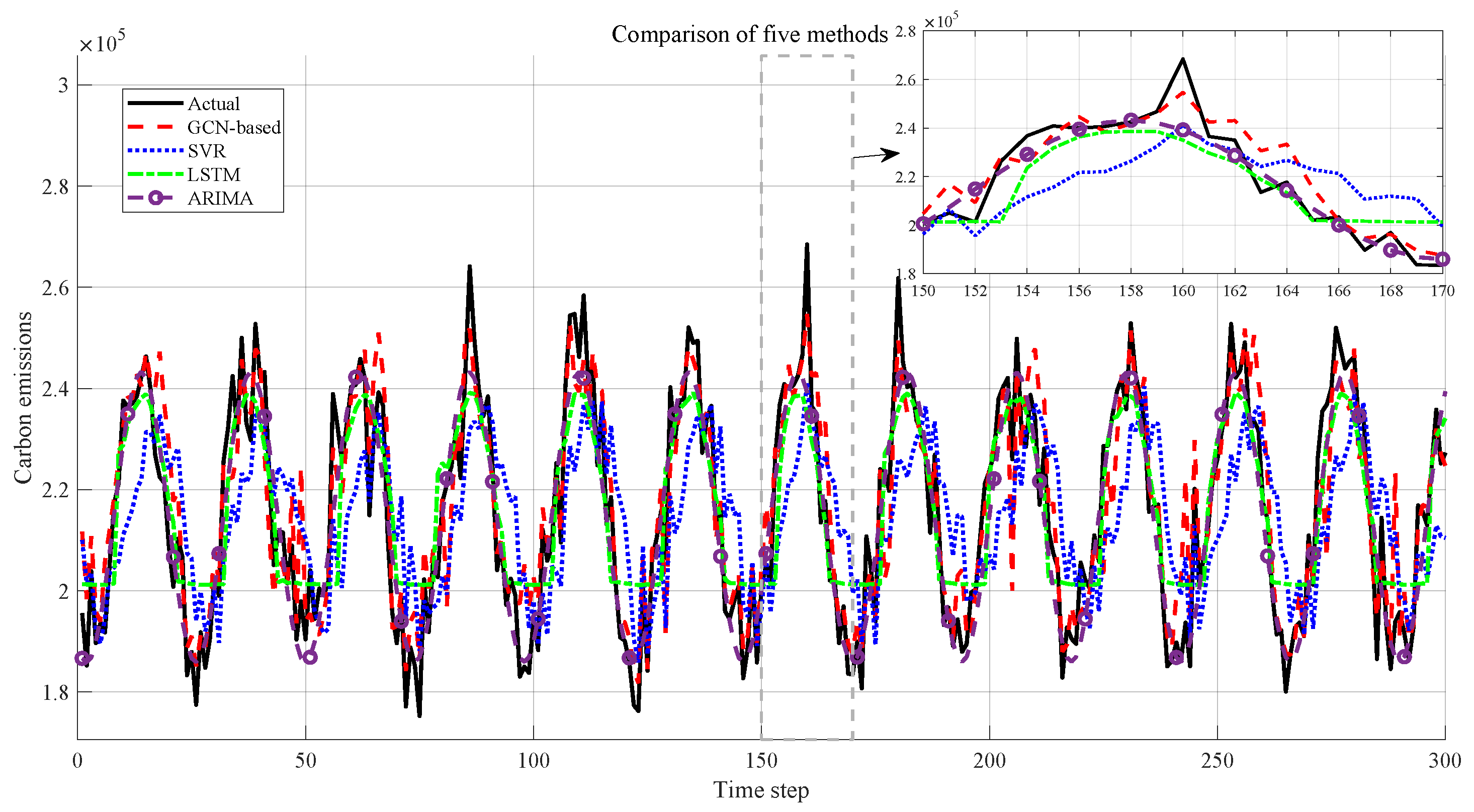
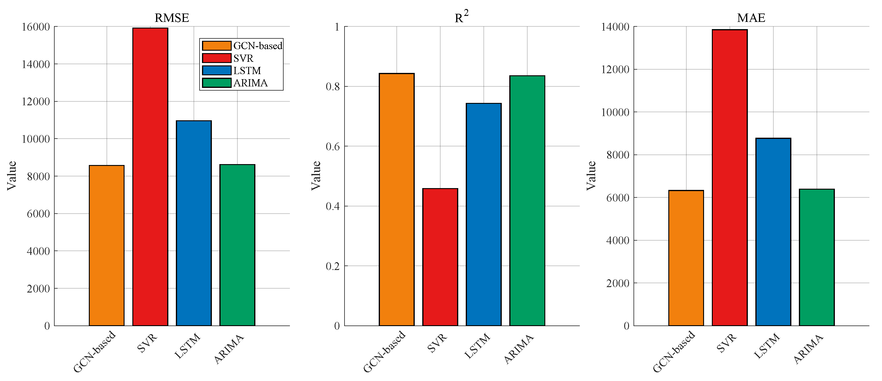
To validate the effectiveness of the proposed model, comparative experiments are against three established baseline models on an identical test set. The experimental results, as illustrated in Figure 10, demonstrate the performance comparison across all methods. The selected benchmark models include support vector regression (SVR), ARIMA, and LSTM networks, representing classical machine learning, traditional time series analysis, and deep learning approaches, respectively. For comprehensive evaluation, three key metrics: RMSE, R 2 , and MAE are computed for all models. The quantitative results are summarized in Table 2, while a comparative bar chart illustrating the performance across these metrics is presented in Figure 11.
Based on the comparative results of key performance metrics presented in Table 2, the proposed model demonstrates superior performance in carbon emission prediction tasks. Specifically, the model achieves a RMSE of 8566.9159 kgCO2, which is significantly lower than that of SVR and LSTM, and slightly better than that of ARIMA. In terms of R2, the proposed model attains the highest value of 0.8431, substantially outperforming SVR and LSTM, and also marginally exceeding ARIMA. Furthermore, for MAE, the proposed model yields 6326.2168 kgCO2, considerably lower than SVR and LSTM, and slightly superior to ARIMA. Collectively, these three key metrics confirm that the proposed model exhibits notable advantages in both prediction accuracy and stability, validating the effectiveness of its integrated graph convolutional and temporal convolutional architecture in capturing complex spatiotemporal dependencies.
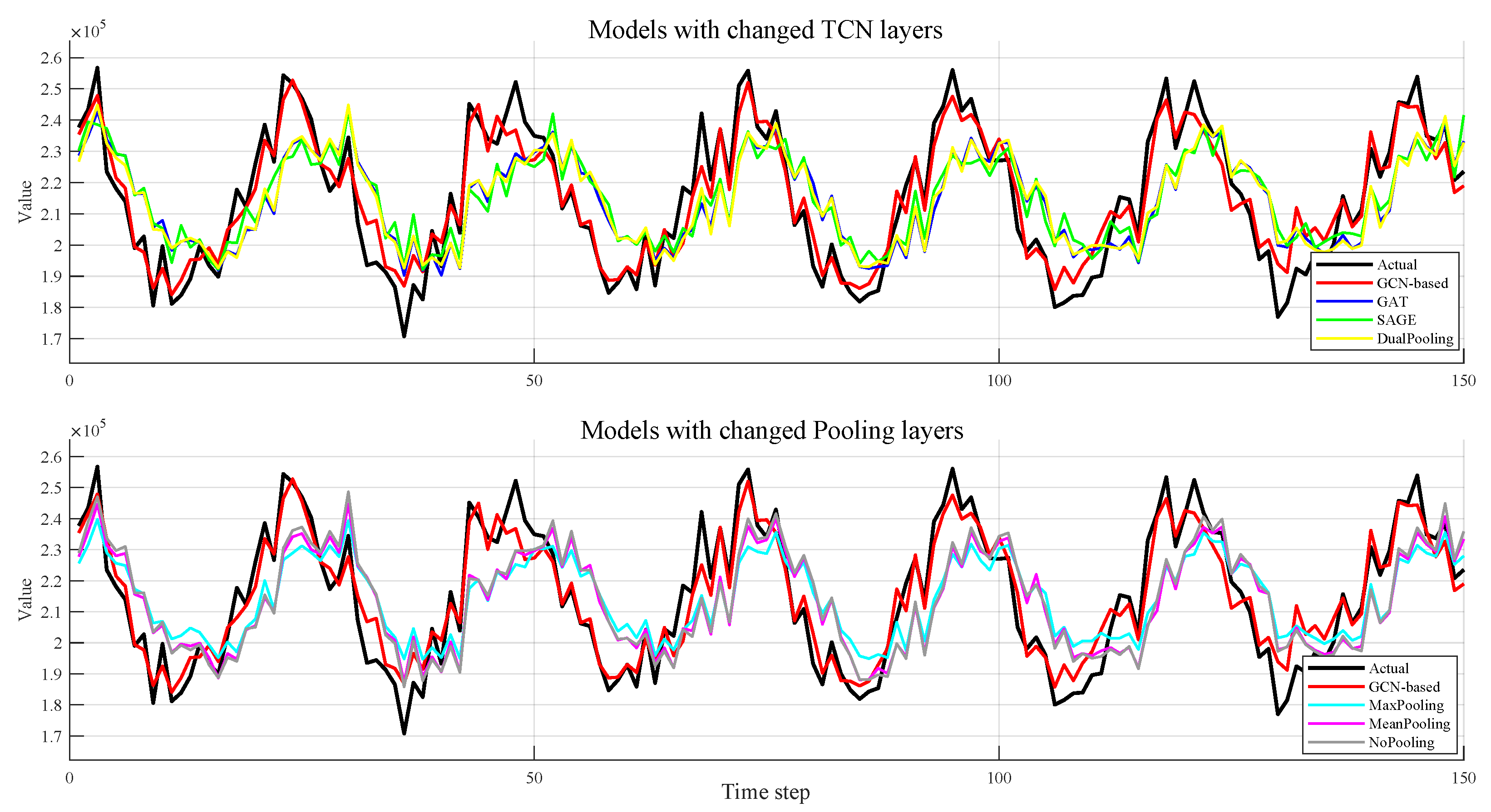
To validate the effectiveness of the proposed GCN-based model for predicting carbon emissions in power systems, a progressive ablation experiment is designed. Using the complete model as a baseline, the TCN layer and pooling layer are sequentially removed or modified to construct six variants. By comparing the performance of each variant across identical datasets and evaluation metrics, the contribution of each model component to prediction accuracy is quantitatively analysed, thereby clarifying their respective essentiality. Table 3 details the configuration of the ablation experiments.
In Table 3, the GCN-GAT model replaces the TCN layer with a graph attention network layer(GAT), while the GCN-SAGE model substitutes the TCN layer with a sampling and aggregation layer. The pooling layer operations categorize pooling into single max-pooling, mean pooling, and no pooling. The experimental results, as illustrated in Figure 12, demonstrate the performance comparison across all ablation experiment models.
The comparative results of the three key performance metrics in the ablation experiment are shown in Figure 13. The proposed GNN-based model achieves the lowest RMSE and MAE, while simultaneously attaining the highest R 2 value, significantly outperforming all ablation variants. This outstanding performance stems from the synergistic integration of mean and max pooling layers with the TCN, which effectively captures both the spatial graph structure and temporal dependencies inherent in carbon emission dynamics. In contrast, models employing a single aggregation mechanism exhibit higher errors due to incomplete graph representation; while removing the TCN leads to a significant performance decline, highlighting the critical role of temporal modeling. Employing alternative aggregators such as GAT or SAGE also results in a slight performance drop, indicating that the combination of standard GCN and TCN provides the most effective feature extraction and sequence modelling approach for this task.

4.2. Robustness Tests

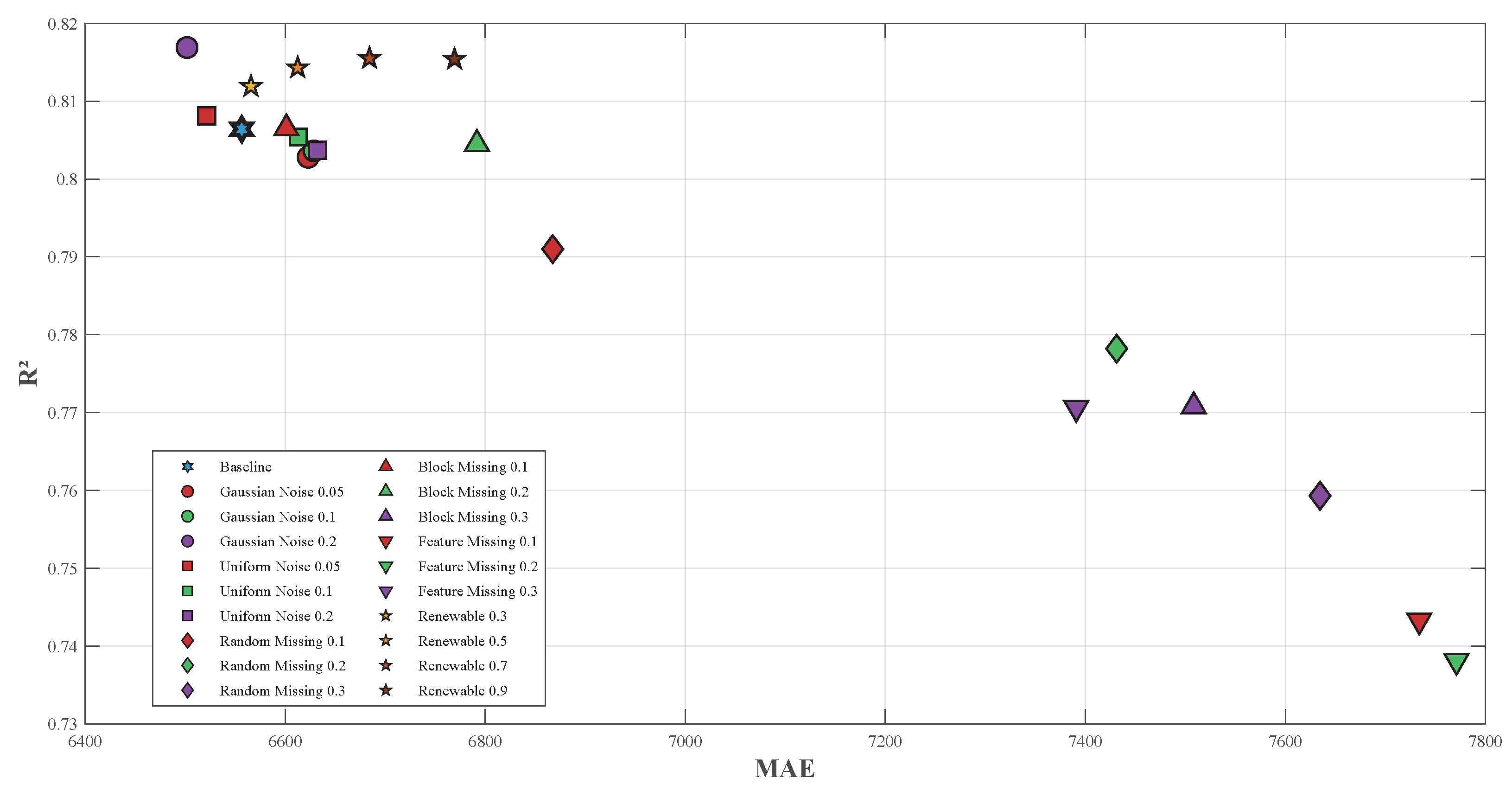
In the real-world grid operating environment, the data acquisition and transmission process is fraught with uncertainty. To ensure the reliability in actual scenarios, robustness testing experiments are required. The proposed GCN-based model is evaluated under various challenging conditions, including data noise, missing data, and operational scenario variations. The corresponding results are systematically presented in Table 4 and Figure 14.
The robustness against data noise is quantified by adding Gaussian and uniform noise to node features, formulated as:
X noisy = X + η · ε , ε N ( 0 , 1 ) or U ( 1 , 1 )
where η is the noise level. In the test, the values of η are 0.05, 0.1 and 0.2 respectively.
As shown in Table 4, the model’s performance metrics exhibit only minor deviations across all tested noise levels. Notably, under Gaussian noise conditions with η = 0.2, the model slightly outperforms the baseline. This indicates that the model’s feature extraction process possesses inherent smoothness and stability, enabling it to effectively filter random disturbances while maintaining performance without significant degradation.
The model is also tested under missing data scenarios, including random, block, and feature-specific missingness. The masking process is defined as:
X missing = M X , M i j Bernoulli ( 1 p )
where p is the missing ratio and ⊙ denotes element-wise multiplication. The elements in M satisfy a Bernoulli distribution. In the test, the values of p are 0.1, 0.2 and 0.3 respectively. Under three scenarios of random missing, block missing, and feature missing, model performance exhibited a reasonable decline with increasing missing rates. When the random missing rate p = 0.3 , the RMSE rose to 10,708.84 kgCO2, while R2 decreased to 0.7593, indicating the model’s sensitivity to high proportions of random missing. However, under block missing ( p = 0.1 ) and feature missing ( p = 0.1 ) conditions, the RMSE values were 9602.47 and 11,060.08 respectively, indicating the model exhibits greater tolerance towards locally continuous missing data than towards globally lost features. These findings indicate that the model partially compensates for local information loss through graph structure propagation mechanisms, yet its adaptability to system-level feature omissions remains subject to improvement.
Additionally, to evaluate the model’s adaptability under different grid operating conditions, operational scenarios with renewable energy penetration rates varying from 30 % to 90 % are simulated. The integration of renewable energy is formulated as:
P g = P g · ( 1 β ) + P renewable , β [ 0.3 , 0.9 ]
where P g represents the original generator output, P g denotes the adjusted output, β indicates the renewable energy penetration rate, and P renewable represents the renewable energy generation. By simulating the gradual increase in renewable energy penetration rates, the model’s capacity to adapt to evolving grid generation structures was assessed using Equation (33). Notably, as the β value increased, the model’s predictive accuracy showed a slight improvement. This indicates that the proposed spatio-temporal model effectively captures the dynamic impact of variable renewable energy integration on carbon emissions, maintaining reliable performance even during significant shifts in generation composition.

5. Conclusions

This paper proposes an innovative GCN-based hybrid framework for real-time prediction of regional carbon emissions. By integrating the structural advantages of graph neural networks with the temporal modeling capabilities of temporal recurrent neural networks, this model effectively addresses the inherent spatiotemporal complexity in power grid carbon emission forecasting. The model first constructs a graph structure representation of the power grid, enabling the GCN component to capture spatial dependencies by aggregating information from neighboring nodes. This enriches feature representations for each node by leveraging contextual information across the entire grid. Concurrently, mean and max pooling operations are employed to enhance the model’s ability to characterize baseline and extreme emission patterns at the graph level, thereby providing a more robust representation of the system’s carbon emission state. On the temporal dimension, the TCN module employs extended causal convolutions to model long-range dependencies while preserving temporal causality. Residual connections within the TCN module further stabilize the training process and enable modeling of deep temporal relationships—crucial for capturing the cumulative nature of carbon emissions over time. Experimental validation on the IEEE 14-node system demonstrates the model’s outstanding performance. Compared to traditional approaches, this framework integrates spatio-temporal modeling into a unified architecture, overcoming the limitations of purely temporal or spatial models. It efficiently handles variable-length sequences and scales to large scale multiregion power systems. Future research will focus on: incorporating renewable energy forecasting uncertainty, extending to multi-energy coupling systems, and exploring practical deployment solutions at regional grid control centers.
Despite its promising performance, the proposed model has certain limitations. First, it relies on accurate and up-to-date grid topology data, which may not always be available in real-time operations. Second, while the model scales well to the IEEE 14-bus system, its computational complexity may increase for larger networks with hundreds of nodes, necessitating further optimization for real-time deployment. Additionally, the current model does not explicitly account for uncertainties in renewable generation or multi-energy interactions, which are critical for practical carbon emission forecasting.
Future research will focus on:
  • Integrating probabilistic forecasting techniques to handle renewable energy uncertainty, such as using Bayesian neural networks or Monte Carlo dropout within the TCN framework.
  • Extending the model to multi-energy coupling systems by incorporating heat and gas network data, using coupled graph structures to capture cross-energy dependencies.
  • Exploring model compression and distributed training strategies to enhance scalability for large-scale power grids.

Author Contributions

Conceptualization, Q.Z.; methodology, X.C.; software, X.C.; validation, X.C.; formal analysis, Q.J.; investigation, C.S.; resources, H.C.; data curation, C.S.; writing—original draft preparation, J.C.; writing—review and editing, H.C.; visualization, Q.J.; supervision, Q.Z.; project administration, Q.Z.; funding acquisition, J.C. All authors have read and agreed to the published version of the manuscript.

Funding

This research received no external funding.

Data Availability Statement

Data are contained within the article.

Conflicts of Interest

Authors Qian Zhao, Jianhua Chen, Qianwei Jia, and Cong Sun were employed by the company State Grid Jibei Electric Power Company Ltd., Beijing, China. The remaining authors declare that the research was conducted in the absence of any commercial or financial relationships that could be construed as a potential conflict of interest.

Abbreviations

The following abbreviations are used in this manuscript:
GCNsGraph Convolutional Networks
TCNsTemporal Convolutional Networks
LEAPLong-range Energy Alternatives Planning
ARIMAAuto-Regressive Integrated Moving Average
LSTMLong Short-Term Memory
SVMSupport Vector Machine
GNNsGraph Neural Networks

References

  1. Li, Y.; Yang, X.; Du, E.; Liu, Y.; Zhang, S.; Yang, C.; Zhang, N.; Liu, C. A review on carbon emission accounting approaches for the electricity power industry. Appl. Energy 2024, 359, 122681. [Google Scholar] [CrossRef]
  2. Albuquerque, B.S.D.; Tostes, M.E.D.L.; Bezerra, U.H.; Carvalho, C.C.M.D.M.; Nascimento, A.L.L.D. Use of Distributed Energy Resources Integrated with the Electric Grid in the Amazon: A Case Study of the Universidade Federal do Pará Poraquê Electric Boat Using a Digital Twin. Machines 2024, 12, 803. [Google Scholar] [CrossRef]
  3. Guo, Z.; Siew, W.H.; Li, Q.; Shi, W. On the Lightning Attachment Process of Wind Turbine–Observation, Experiments and Modelling. Machines 2025, 13, 704. [Google Scholar] [CrossRef]
  4. Yang, L.; Mei, L.; Chen, Y.; Hao, Y.; Li, L.; Wu, J.; Mao, X. Prediction Method for Mechanical Characteristic Parameters of Weak Components of 110 kV Transmission Tower under Ice-Covered Condition Based on Finite Element Simulation and Machine Learning. Machines 2024, 12, 652. [Google Scholar] [CrossRef]
  5. Li, P.; Wu, W.; Wang, X.; Xu, B. A Data-Driven Linear Optimal Power Flow Model for Distribution Networks. IEEE Trans. Power Syst. 2023, 38, 956–959. [Google Scholar]
  6. Tian, P.; Jin, Y.; Xie, N.; Wang, C.; Huang, C. Power Flow Calculation for VSC-Based AC/DC Hybrid Systems Based on Fast and Flexible Holomorphic Embedding. J. Mod. Power Syst. Clean Energy 2024, 12, 1370–1382. [Google Scholar]
  7. Ma, M.; Li, Y.; Du, E.; Jiang, H.; Zhang, N.; Wang, W.; Wang, M. Calculating Probabilistic Carbon Emission Flow: An Adaptive Regression-Based Framework. IEEE Trans. Sustain. Energy 2024, 15, 1576–1588. [Google Scholar] [CrossRef]
  8. Zhang, X.; Zhu, H.; Cheng, Z.; Shao, J.; Yu, X.; Jiang, J. A review of carbon emissions accounting and prediction on the power grid. Electr. Eng. 2025, 107, 7561–7574. [Google Scholar] [CrossRef]
  9. Wang, T.; Watson, J. Scenario analysis of China’s emissions pathways in the 21st century for low carbon transition. Energy Policy 2010, 38, 3537–3546. [Google Scholar] [CrossRef]
  10. McPherson, M.; Karney, B. Long-term scenario alternatives and their implications: LEAP model application of Panama’s electricity sector. Energy Policy 2014, 68, 146–157. [Google Scholar] [CrossRef]
  11. Maji, D.; Shenoy, P.; Sitaraman, R.K. Multi-Day Forecasting of Electric Grid Carbon Intensity Using Machine Learning. ACM SIGENERGY Energy Inform. Rev. 2023, 3, 19–33. [Google Scholar]
  12. Luo, J.; Zhuo, W.; Liu, S.; Xu, B. The Optimization of Carbon Emission Prediction in Low Carbon Energy Economy Under Big Data. IEEE Access 2024, 12, 14690–14702. [Google Scholar] [CrossRef]
  13. Lau, E.; Yang, Q.; Forbes, A.; Wright, P.; Livina, V. Modelling carbon emissions in electric systems. Energy Convers. Manag. 2014, 80, 573–581. [Google Scholar] [CrossRef]
  14. Wang, H.; Li, B.; Khan, M.Q. Prediction of Shanghai Electric Power Carbon Emissions Based on Improved STIRPAT Model. Sustainability 2022, 14, 13068. [Google Scholar] [CrossRef]
  15. Chen, J.; Zheng, L.; Che, W.; Liu, L.; Huang, H.; Liu, J.; Xing, C.; Qiu, P. A method for measuring carbon emissions from power plants using a CNN-LSTM-Attention model with Bayesian optimization. Case Stud. Therm. Eng. 2024, 63, 105334. [Google Scholar]
  16. Leerbeck, K.; Bacher, P.; Junker, R.G.; Goranović, G.; Corradi, O.; Ebrahimy, R.; Tveit, A.; Madsen, H. Short-term forecasting of CO2 emission intensity in power grids by machine learning. Appl. Energy 2020, 277, 115527. [Google Scholar] [CrossRef]
  17. Han, Z.; Cui, B.; Xu, L.; Wang, J.; Guo, Z. Coupling LSTM and CNN Neural Networks for Accurate Carbon Emission Prediction in 30 Chinese Provinces. Sustainability 2023, 15, 13934. [Google Scholar] [CrossRef]
  18. Qiao, W.; Lu, H.; Zhou, G.; Azimi, M.; Yang, Q.; Tian, W. A hybrid algorithm for carbon dioxide emissions forecasting based on improved lion swarm optimizer. J. Clean. Prod. 2020, 244, 118612. [Google Scholar] [CrossRef]
  19. Wei, X.; Xu, Y. Research on carbon emission prediction and economic policy based on TCN-LSTM combined with attention mechanism. Front. Ecol. Evol. 2023, 11, 1270248. [Google Scholar] [CrossRef]
  20. Han, Y.; Hao, Y.; Feng, M.; Chen, K.; Xing, R.; Liu, Y.; Lin, X.; Ma, B.; Fan, J.; Geng, Z. Novel STAttention GraphWaveNet model for residential household appliance prediction and energy structure optimization. Energy 2024, 307, 132582. [Google Scholar]
  21. Lopez-Garcia, T.B.; Domínguez-Navarro, J.A. Optimal Power Flow With Physics-Informed Typed Graph Neural Networks. IEEE Trans. Power Syst. 2025, 40, 381–393. [Google Scholar] [CrossRef]
  22. Wu, T.; Zhang, Y.J.A.; Liu, Y.; Lau, W.C.; Xu, H. Missing Data Recovery in Large Power Systems Using Network Embedding. IEEE Trans. Smart Grid 2021, 12, 680–691. [Google Scholar] [CrossRef]
  23. Wu, T.; Scaglione, A.; Arnold, D. Complex-Value Spatiotemporal Graph Convolutional Neural Networks and Its Applications to Electric Power Systems AI. IEEE Trans. Smart Grid 2024, 15, 3193–3207. [Google Scholar] [CrossRef]
  24. Hossain, R.R.; Huang, Q.; Huang, R. Graph Convolutional Network-Based Topology Embedded Deep Reinforcement Learning for Voltage Stability Control. IEEE Trans. Power Syst. 2021, 36, 4848–4851. [Google Scholar] [CrossRef]
  25. Chen, L.; Zhou, S.; Liang, X.; Lu, W.; Xia, M.; Weng, L.; Geng, J.; Liu, J. Predicting Power Dispatch for Unit Commitment Problems Using Graph-Temporal Convolutional Networks With Constrained Learning. IEEE Trans. Ind. Inform. 2025, 21, 5734–5745. [Google Scholar] [CrossRef]
  26. Li, Y.; Song, L.; Zhang, S.; Kraus, L.; Adcox, T.; Willardson, R.; Komandur, A.; Lu, N. A TCN-Based Hybrid Forecasting Framework for Hours-Ahead Utility-Scale PV Forecasting. IEEE Trans. Smart Grid 2023, 14, 4073–4085. [Google Scholar]
  27. Zhou, X.; Pang, C.; Zeng, X.; Jiang, L.; Chen, Y. A Short-Term Power Prediction Method Based on Temporal Convolutional Network in Virtual Power Plant Photovoltaic System. IEEE Trans. Instrum. Meas. 2023, 72, 1–10. [Google Scholar] [CrossRef]
  28. Wang, Y.; Chen, J.; Chen, X.; Zeng, X.; Kong, Y.; Sun, S.; Guo, Y.; Liu, Y. Short-Term Load Forecasting for Industrial Customers Based on TCN-LightGBM. IEEE Trans. Power Syst. 2021, 36, 1984–1997. [Google Scholar]
  29. Ramos, A.C.S.; Freitas, F.D.; Zizzo, G. Economic Dispatch Problem Solution via Holomorphic Embedding Method on IEEE 14-Bus System for Different Loading Scenarios. IEEE Trans. Ind. Appl. 2024, 60, 2664–2672. [Google Scholar] [CrossRef]
  30. Vazquez-Rodriguez, S.; Duro, R. A genetic based technique for the determination of power system topological observability. In Proceedings of the Second IEEE International Workshop on Intelligent Data Acquisition and Advanced Computing Systems: Technology and Applications, Lviv, Ukraine, 8–10 September 2003; pp. 48–52. [Google Scholar]
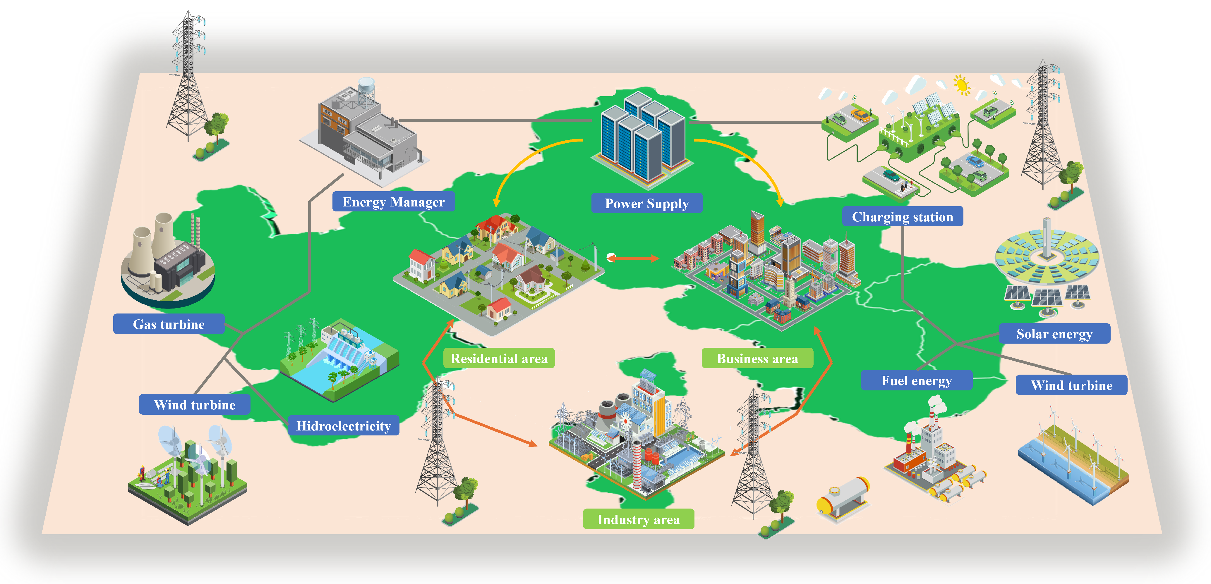
Figure 1. The operation process of the power grid.
Machines 13 01061 g001
Figure 2. A topology structure of power grids.
Machines 13 01061 g002
Figure 3. Schematic depiction of multi-layer Graph Convolutional Networks.
Machines 13 01061 g003
Figure 4. The architecture of the proposed GCN-based carbon emissions prediction approach.
Machines 13 01061 g004
Figure 5. Structure of a GCN layer.
Machines 13 01061 g005
Figure 6. The operation of Pooling Layer.
Machines 13 01061 g006
Figure 7. A dilation causal convolution to extract temporal features layer by layer.
Machines 13 01061 g007
Figure 8. A causal dilation temporal convolution to extract temporal features layer by layer.
Machines 13 01061 g008
Figure 9. IEEE 14-bus electric power systems [30].
Machines 13 01061 g009
Figure 10. The comparison experimental results.
Machines 13 01061 g010
Figure 11. The key metrics bar charts for different models.
Machines 13 01061 g011
Figure 12. The results of ablation experiments.
Machines 13 01061 g012
Figure 13. The results of ablation experiments.
Machines 13 01061 g013
Figure 14. Model Performance under robustness test scenarios.
Machines 13 01061 g014
Table 1. Power Generation Statistics for Generating Nodes.
NodeAverage Power Output (MW)
1232.14
237.76
31.99
62.07
82.10
Table 2. Comparison of key metrics across different models.
ModelRMSE (kgCO2)R2MAE (kgCO2)
GCN-based8566.91590.84316326.2168
SVR15,918.24160.458413,854.6673
LSTM10,963.14220.74318769.0145
ARIMA8618.39740.83566390.3763
Table 3. Configuration of ablation experiment models.
ModelPooling StrategyTCN LayerGCN Layer
GCN-basedDual PoolingTCNGCN
GCN-GATDual PoolingNoGAT
GCN-SAGEDual PoolingNoSAGE
DualPoolingDual PoolingNoGCN
MaxPoolingMax PoolingNoGCN
MeanPoolingMean PoolingNoGCN
NoPoolingNo PoolingNoGCN
Table 4. The comparative results of the robustness experiments.
ModelRMSE (kgCO2)MAE (kgCO2)R2
Baseline9605.016556.590.8064
Gaussian Noise 0.059693.926622.940.8028
Gaussian Noise 0.19674.886628.840.8036
Gaussian Noise 0.29340.276501.820.8169
Uniform Noise 0.059561.436521.510.8081
Uniform Noise 0.19629.726613.130.8054
Uniform Noise 0.29672.016632.330.8037
Random Missing 0.19978.916867.450.7910
Random Missing 0.210,279.397431.310.7782
Random Missing 0.310,708.847634.640.7593
Block Missing 0.19602.476601.190.8065
Block Missing 0.29664.986791.650.8040
Block Missing 0.310,450.407508.430.7708
Feature Missing 0.111,060.087733.860.7433
Feature Missing 0.211,170.177771.100.7381
Feature Missing 0.310,454.127390.900.7706
Renewable 0.39470.386565.780.8119
Renewable 0.59413.376612.500.8143
Renewable 0.79385.586684.250.8155
Renewable 0.99389.306769.280.8154
Disclaimer/Publisher’s Note: The statements, opinions and data contained in all publications are solely those of the individual author(s) and contributor(s) and not of MDPI and/or the editor(s). MDPI and/or the editor(s) disclaim responsibility for any injury to people or property resulting from any ideas, methods, instructions or products referred to in the content.