Ball Mill Load Classification Method Based on Multi-Scale Feature Collaborative Perception

Abstract

Against the backdrop of intelligent manufacturing, the ball mill, as a key energy-consuming piece of equipment, requires an accurate perception of its load state, which is crucial for optimizing production efficiency and ensuring operational safety. However, its vibration signals exhibit typical nonlinear and non-stationary characteristics, intertwined with complex noise, posing significant challenges to high-precision identification. A core contradiction exists in existing diagnostic methods: convolution network-based methods excel at capturing local features but overlook global trends, while Transformer-type models, although capable of capturing long-range dependencies, tend to “average out” critical local transient information during modeling. To address this dilemma, this paper proposes a new paradigm for multi-scale feature collaborative perception. This paradigm is implemented through an innovative deep learning architecture—the Residual Block-Swin Transformer Network (RB-SwinT). This architecture subtly achieves hierarchical and in-depth integration of the powerful global context modeling capability of Swin Transformer and the excellent local detail refinement capability of the residual module (ResBlock), enabling synchronous and efficient representation of both the macro trends and micro mutations of signals. On the experimental dataset covering nine types of fine operating conditions, the overall recognition accuracy of the proposed method reaches as high as 96.20%, which is significantly superior to a variety of mainstream models. To further verify the model’s generalization ability, this study was tested on the CWRU public bearing fault dataset, achieving a recognition accuracy of 99.36%, which outperforms various comparative methods such as SAVMD-CNN. This study not only provides a reliable new technical approach for ball mill load identification but also demonstrates its practical application value in indicating critical operating conditions and optimizing production operations through an in-depth analysis of the physical connotations of each load level. More importantly, its “global-local” collaborative modeling concept opens up a promising technical path for processing a broader range of complex industrial time-series data.

1. Introduction

Against the backdrop of Industry 4.0 and the wave of intelligent manufacturing, condition monitoring and predictive maintenance for heavy rotating equipment have become core technical links to ensure production safety and improve energy efficiency [1]. As a key energy-consuming equipment in fields such as mining and metallurgy, the operating state of the ball mill directly determines product quality and production line efficiency; therefore, the implementation of accurate load identification for it holds significant theoretical and engineering value [2]. However, the complex dynamic processes of multi-body collision inside the ball mill and the coupling between materials and media result in its vibration signals exhibiting typical nonlinear and non-stationary characteristics [3]. The essence of this challenge stems from an inherent contradiction in the signal itself: a stable grinding process manifests as a long-range dependent global trend, while the transient changes in load present as high-frequency, short-duration local transient features [4]. How to collaboratively capture information of these two scales within a unified framework has long been a core problem in this field.

To address this dilemma, early studies mainly focused on traditional machine learning methods, such as Support Vector Machine (SVM) [5] and Variational Mode Decomposition (VMD) [6]. Such methods are highly dependent on manually designed feature engineering, but when processing ball mill vibration signals with significant nonlinear and non-stationary characteristics, manually designed features cannot fully adapt to the dynamic changes in the signals, resulting in limited generalization ability of the models.

With the aim of surmounting these limitations, researchers have ventured into exploring intelligent diagnosis methods capable of automatic feature learning [7]. In recent years, Deep Learning (DL), leveraging its powerful nonlinear function approximation capability, has become the mainstream technical approach for ball mill load signal processing [8]. Through a multi-layer architecture, neural networks automatically learn abstract features from signals and establish complex mappings between the mill’s characteristic parameters and load states, demonstrating robust performance in scenarios where signals are subject to strong interference. Many researchers have conducted explorations in this direction: Cai et al. [9] addressed the issue of insufficient accuracy in ball mill load identification, proposed a UMAP-XGBoost multi-domain feature segmentation identification method. By integrating multi-domain features and optimizing the model, they enhanced the method’s robustness and classification accuracy, achieving superior load identification results. Liu et al. [10] aimed to solve problems of traditional prediction models, such as poor interpretability, low prediction efficiency, and insufficient generalization ability caused by data distribution differences, and proposed a multi-task ball mill load parameter prediction model that integrates physical information and domain adaptation. While improving prediction accuracy, this model effectively adapts to variable operating conditions. Huang et al. [11] further addressed the problems that the traditional D-S evidence theory tends to produce counterintuitive results when dealing with conflicting evidence, and the insufficient accuracy of ball mill load soft sensing. They proposed a new load identification method based on a novel evidence dissimilarity measurement index, an improved evidence combination method, and an improved multi-classifier ensemble modeling. Specifically, a laboratory-scale ball mill was taken as the research object, and bearing housing vibration signals were selected as auxiliary variables; the effect of conflicting evidence processing was optimized via the novel evidence dissimilarity measurement index; recognition results from multiple classifiers and multi-sensors were fused using the improved evidence combination method, ultimately achieving accurate soft sensing of ball mill load. Luo et al. [12] proposed a fusion method combining improved Empirical Wavelet Transform (EWT)-multiscale entropy and Kernel Extreme Learning Machine (KELM). By optimizing the EWT spectrum segmentation strategy, the reconstructed multiscale entropy was used as the load feature vector, significantly improving the accuracy of ball mill load identification. Despite the phased progress achieved by the aforementioned studies, existing ball mill load identification methods—especially deep learning methods with CNNs (Convolutional Neural Networks) or ResNet as backbone feature extraction networks—still have three core limitations when processing ball mill vibration signals:

(1)

Insufficient global correlation capture by CNNs: Although CNNs [13] excel at extracting local spatial features, ball mill load variation is a typical time-series dynamic process, and the spectral features at different time steps exhibit strong correlations. However, CNNs struggle to effectively capture the global correlation information in the “time-frequency” dimension.

(2)

Limited high-frequency detail extraction and noise resistance of ResNet: ResNet [14] alleviates the gradient vanishing problem of deep networks through residual connections. Nevertheless, under the interference of complex industrial noise, its ability to identify high-frequency vibration details (such as spectral spikes during sudden load changes) is weak, and these details are easily submerged by noise.

Thus, the Attention Mechanism capable of capturing long-range dependencies has begun to attract attention and has been proven effective in improving the performance of diagnostic models [15]. To address the limitation of CNNs in global perception, researchers have begun to introduce the Transformer architecture from the field of computer vision into industrial diagnosis. In the field of industrial equipment monitoring, signal analysis techniques have demonstrated favorable effectiveness in similar equipment such as crushers, providing important insights for ball mill load monitoring: Wyłomanska et al. [16] combined time-series analysis, spectrograms, and classical envelope analysis, successfully applying this approach to eliminate impulse noise from vibration signals of copper ore crushers, which significantly improved the sensitivity of equipment damage detection. Zak et al. [17] processed the impulse spectrograms of crushers using fractional lower-order covariance; this method not only completed the fault detection task but also accurately located the key frequency bands (information bands) containing fault information. Tanaś et al. [18] identified the natural frequency of grain crushers, conducted in-depth analysis of their dynamic characteristics and damping parameters, and ultimately realized the optimization of the equipment’s acoustic properties. These advancements provide methodological support for industrial signal processing. However, the nonlinearity, non-stationarity, and interference complexity of ball mill vibration signals are far more pronounced than those of ordinary crushers, requiring the targeted design of more adaptive models. In 2021, the Swin Transformer proposed by Liu et al. [19] offered a new technical direction for addressing this issue: its “shifted windows” mechanism reduces the computational complexity from the square order of the input size to the linear order through self-attention calculation within local windows and window shifting in cascaded layers. Moreover, the non-overlapping window design is more compatible with hardware deployment, balancing efficiency and performance. Meanwhile, by merging adjacent modules to construct hierarchical feature maps, it can be adapted to various visual tasks. However, directly applying the standard Transformer model for industrial diagnosis reveals a critical flaw: when the global self-attention mechanism balances all input information, it may inadvertently “smooth out” or “average out” the high-frequency transient spikes that serve as key indicators of load changes. Therefore, a fundamental gap remains: currently, there is a lack of a solution capable of collaboratively modeling both the “forest” (global trends) and the “trees” (local transients) within a unified architecture.

To fill this critical gap and address the aforementioned core contradictions, a new “multi-scale feature collaborative perception” paradigm for intelligent diagnosis is proposed and validated, with the core objective of overcoming the limitations of existing models in collaboratively processing global trends and local details. To achieve this objective, an innovative Residual Swin Transformer Network (RB-SwinT) architecture is introduced. This architecture subtly integrates a residual module (ResBlock) after each stage of the Swin Transformer. Herein, the Swin Transformer backbone network serves as a powerful long-range feature extractor, responsible for capturing global context; while the residual module acts as a local feature refiner, tasked with preserving and enhancing key transient details that might be lost in other models. The main contributions of this paper are as follows:

(1)

An innovative RB-SwinT architecture is designed, realizing for the first time the synchronous and efficient modeling of both “global trends” and “local details” in the time-frequency maps of vibration signals.

(2)

The problem of classifying one-dimensional industrial vibration signals is successfully transformed into a two-dimensional visual time-frequency map recognition task, and the great application potential of advanced visual Transformer architectures in this field is verified.

(3)

Dual experimental validation was conducted on the self-constructed ball mill load dataset and the internationally recognized CWRU bearing fault dataset. Experimental results demonstrate that the proposed model not only achieves an accuracy of 96.20% in the 9-class ball mill load identification task but also reaches an accuracy of 99.36% in the 10-class CWRU bearing fault diagnosis task.

(4)

This study has conducted an in-depth analysis of the correlation between the refined recognition results of the model and the physical connotations of load states, explored its application value in indicating critical operating conditions and optimizing operating parameters, thereby enhancing the interpretability and application potential of this method in practical industrial environments.

2. Theoretical Basis

2.1. Short-Time Fourier Transform (STFT) for Time-Frequency Feature Conversion

The Fourier transform only reflects the frequency-domain characteristics of a signal and cannot be used to analyze the signal in the time domain. To establish a connection between the time domain and frequency domain, the Short-Time Fourier Transform (STFT) was proposed. As a joint time-frequency analysis method for non-stationary signals, the STFT converts one-dimensional time-domain signals into two-dimensional time-frequency images, intuitively revealing the law of how signal frequency components evolve over time. This enables the simultaneous visualization of both the global trends of the mill’s operating state and the local transient features caused by load changes. Its feature spectrum contains information from both the time domain and frequency domain, and it is essentially a windowed Fourier transform. It uses a fixed-length window function to slide over the time-domain signal, intercept segments of the signal, and perform Fourier transforms on these segments to obtain a set of local spectra for each time period [20]. Its calculation formula is as follows:

$$STFT(t,f)={\displaystyle {\int }_{-\infty }^{\infty }x(\tau )}w(\tau -t)e^{-j2\pi f\tau }d\tau$$

(1)

where x(τ) represents the one-dimensional time-domain signal, τ and f denote time and frequency, respectively, and w(τ – t) signifies an analytical window function centered at time t.

The time resolution and frequency resolution of the spectrum obtained by STFT depend on the length of the window function: the longer the window length, the lower the time resolution and the higher the frequency resolution. Since it cannot adjust the window size autonomously, it is necessary to select an optimal window to better analyze the time-frequency characteristics of the ball mill. Although STFT cannot balance time resolution and frequency resolution, it is still widely used in practical engineering due to its simple calculation. According to the uncertainty principle, the time-bandwidth product has a lower bound, namely ΔtΔω ≥ 1/2, and the only function that can reach this lower bound is the Gaussian function. Therefore, in practical applications, the Gaussian.

2.2. Residual Block for Gradient Propagation in Deep Networks

The Residual Block is a fundamental building unit in the Deep Residual Network (ResNet). Proposed by He et al. [21], ResNet is a classic deep learning neural network model that adopts the concept of residual learning. This design enables a significant increase in the depth of the neural network without causing performance degradation. In the diagnostic paradigm of this study, the Residual Block plays a crucial role as a “local feature refiner,” whose core task is to ensure that key detailed information representing transient load changes is not “smoothed out” or lost when passing through the deep network. As the basic unit for implementing this concept, each Residual Block consists of two or three convolutional layers. As shown in Figure 1, it introduces a “shortcut connection” [22], which directly adds the input to the output of the convolutional layers. This design allows the network to easily learn the residual part, thereby enabling better optimization and training of the deep network.

Beyond its well-known advantages, such as addressing the gradient vanishing problem and avoiding overfitting, a more important role of this structure is that it provides a “green channel” for the lossless transmission of fine-grained features. In deep learning neural networks, calculating gradient values via the backpropagation algorithm is a critical step. However, as the network depth increases, gradients become progressively smaller and eventually vanish, rendering the neural network unoptimizable. The shortcut connections in Residual Blocks enable gradients to propagate directly to earlier layers, solving the gradient vanishing problem. This means that even when the deep backbone network (such as Swin Transformer) is focused on learning global patterns, the local, high-frequency, detailed features captured by Residual Blocks can be effectively preserved and enhanced—greatly improving the diagnostic accuracy and robustness of the entire model.

2.3. The Swin Transformer Network Model for Hierarchical Processing of Image Features

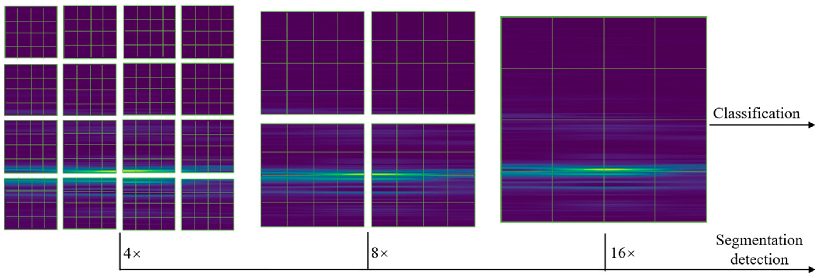
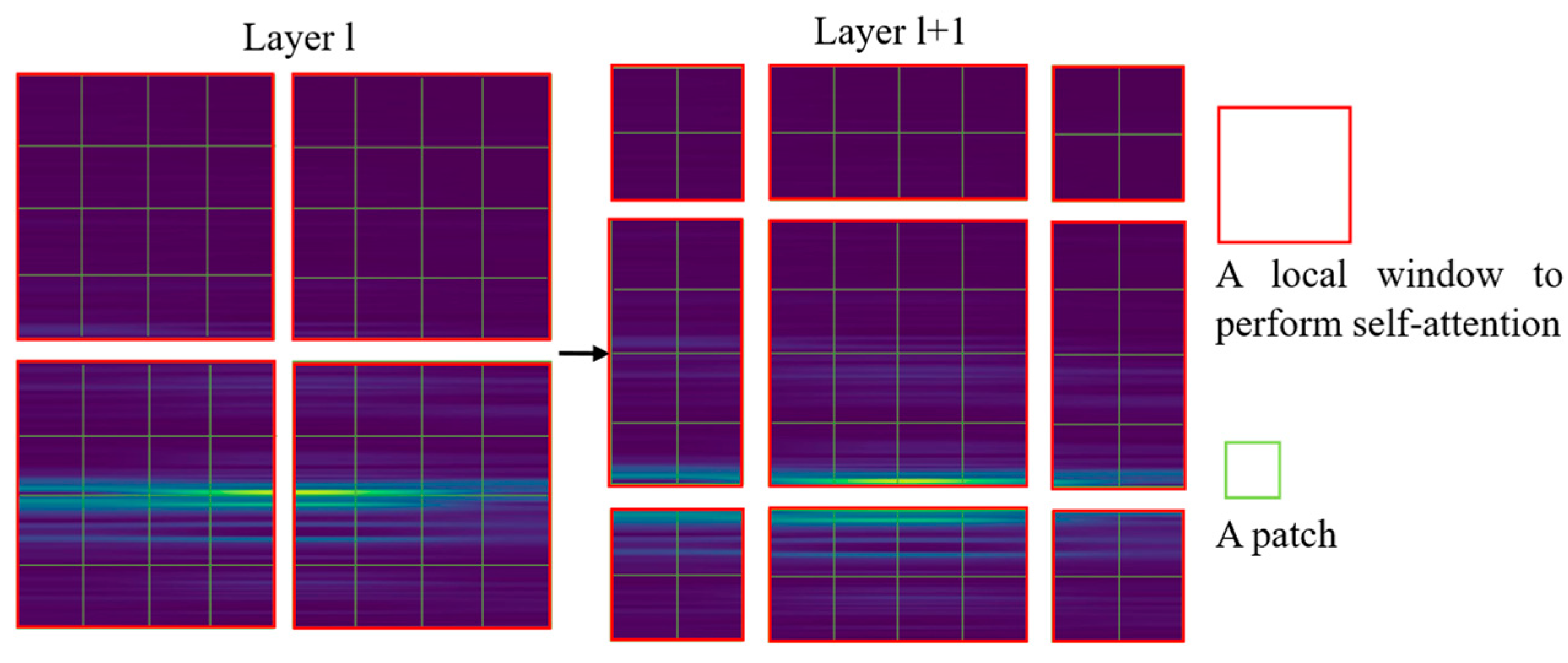
The Swin Transformer network model is a deep learning model based on the attention mechanism, which exhibits excellent performance in image recognition and computer vision tasks. In the diagnostic paradigm of this study, the Swin Transformer is selected as the backbone network for feature extraction, and its core role is to serve as an efficient “global context modeler,” responsible for capturing the long-range dependencies and overall trends of the mill’s operating state from time-frequency maps. As shown in Figure 2, the Swin Transformer adopts a brand-new hierarchical structure. Unlike traditional vision Transformers, it constructs features through the “shifted windows” mechanism illustrated in Figure 3. This design includes non-overlapping local windows and overlapping cross-windows, cleverly confining the computationally expensive self-attention calculations within each small window while enabling the interaction of window information across different levels. This strategy not only significantly improves the efficiency of the model in processing high-resolution images (such as our time-frequency maps) but, more importantly, it can gradually build a global perspective of the entire image while maintaining sensitivity to local information.

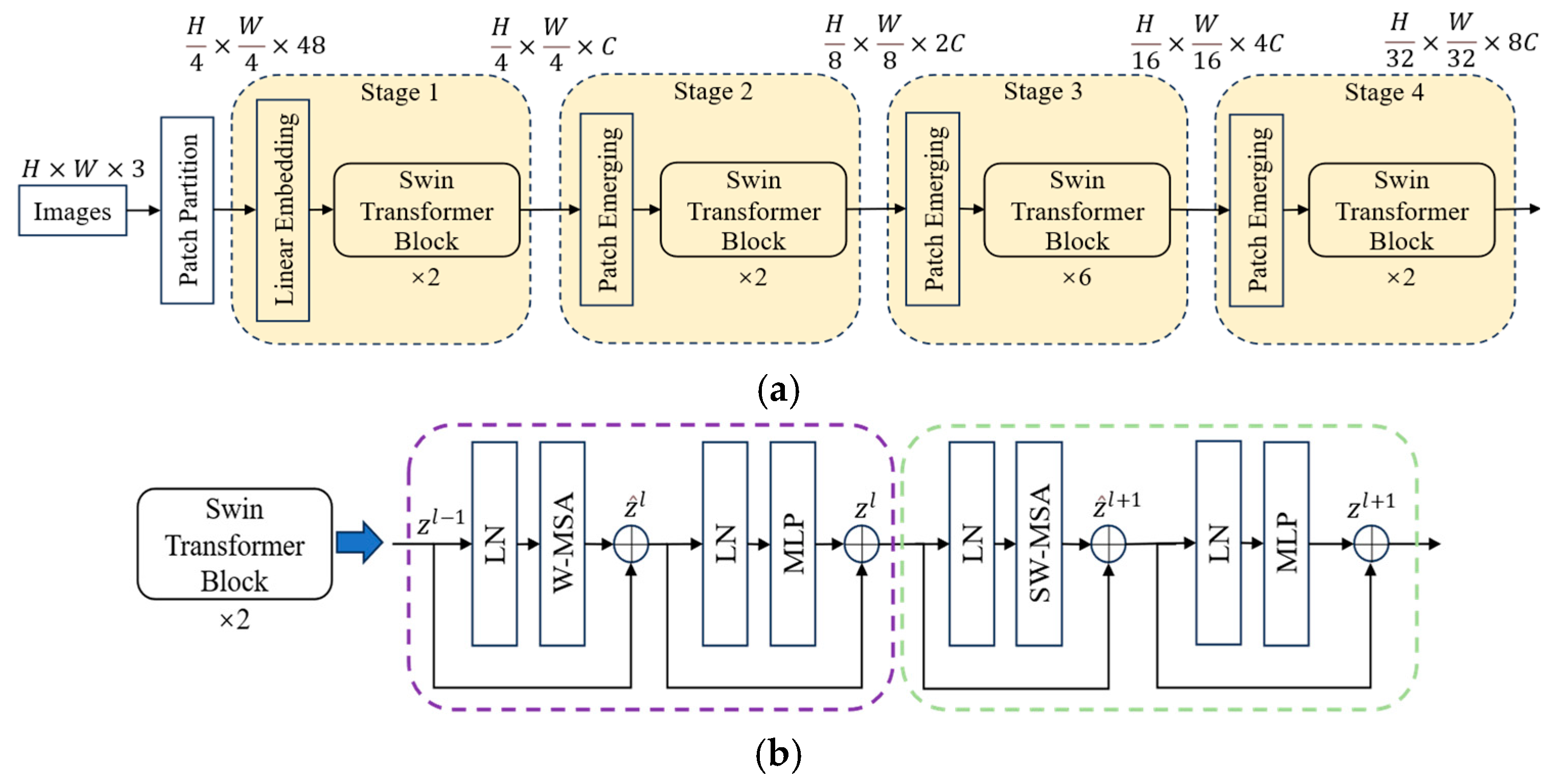
The structure of the Swin Transformer model, as shown in Figure 4, mainly consists of an image patch partition layer, stacked modules, a normalization layer, a global pooling layer, and a fully connected layer. The input image is divided into numerous small image patches, with each patch treated as a “token”. These image patches are passed as inputs to the Swin Transformer model, and multi-layer Transformer modules are used to process feature representations at different levels. The core of these Transformer modules is the self-attention mechanism. It is this mechanism that endows the model with the ability to understand the relationships between any two parts of the image, allowing it to surpass the limitation of the local receptive field of traditional CNNs. Thus, the model is perfectly capable of capturing the global evolution patterns of signals.

3. The Proposed Method

3.1. Overall Architecture and Design Philosophy

Most of the previously proposed feature extraction methods for ball mill load identification are based on one-dimensional vibration data [23]. Although such methods can preserve the nonlinear features of signals to a certain extent, they often struggle to fully exploit the discriminative information in high-dimensional features and lack effective modeling of the dynamic contextual correlations contained in the original vibration signals within the time series. In recent years, converting one-dimensional signals into two-dimensional images via time-frequency analysis and then using deep visual models for feature extraction has become an important research direction in state identification of complex mechanical systems. In the study of Reference [24], researchers integrated multi-domain features of vibration signals through a TF-MDA model with parallel one-dimensional CNN modules, thereby improving fault classification accuracy. Reference [25] adopted the Wigner-Ville Distribution (WVD) method to visualize acoustic signals for extracting vibration signal features, and combined it with an artificial neural network-based fault identification method to realize fault diagnosis of brushless motors—fully demonstrating the advantages of time-frequency image representation in non-stationary signal processing. Based on this, converting one-dimensional vibration signals into two-dimensional time-frequency images is of significant necessity: on the one hand, time-frequency transforms (such as STFT) can more completely preserve the dynamic features of the original signal in the joint time-frequency domain, providing richer discriminative information than a single dimension; on the other hand, the image-based representation facilitates the introduction of powerful visual recognition models (such as Swin Transformer), thereby leveraging their structural advantages to enhance the simultaneous representation and generalization capabilities for both “global trends” and “local details” in the signal.

Based on the above reasons, this paper proposes to use STFT to convert one-dimensional ball mill vibration signals into two-dimensional time-frequency maps, which are then input into the RB-SwinT model—specifically designed in this study to solve the challenge of collaborative modeling of “global-local” features—for feature extraction and load state classification. By collaboratively capturing long-range dependencies (global trends) and transient details (local features) in time-frequency maps, this architecture significantly improves the accuracy and robustness of load identification. The ball mill load identification algorithm based on STFT and RB-SwinT mainly consists of three steps: first, the original vibration signals are converted into time-frequency images using STFT; second, the dataset is divided into a training set and a test set at a ratio of 4:1; finally, the image data is input into the RB-SwinT model for end-to-end feature extraction and load classification.

3.2. RB-SwinT Collaborative Perception Architecture

The design philosophy of the RB-SwinT architecture is precisely to realize the “global-local collaborative perception” paradigm described in the introduction. It is not a simple stack of modules, but a deep fusion with complementary functions: the Swin Transformer is used as a global context extractor, and ResBlocks are subtly integrated as local detail refiners. As shown in Figure 5a, a ResBlock module is integrated after each stage of the Swin Transformer. Leveraging its classic cross-layer connections and residual learning capabilities, this module serves two core purposes: First, from a technical perspective, it ensures the trainability of the entire complex model by alleviating the gradient vanishing problem in deep networks. Second, from a feature perspective—which is the key to our design—it provides a “highway” for information transmission of these fine local transient features, ensuring that such critical details do not attenuate or obtain lost in the deep network. This design, where “the backbone captures trends and residuals preserve details,” forms a perfect functional complement to the hierarchical attention mechanism of the Swin Transformer, greatly enhancing the model’s ability to comprehensively represent heterogeneous information in time-frequency maps.

In the ResBlock structure shown in Figure 5b, let the input be x, the expected mapping be H(x), and after passing through the stacked convolutional layers in the ResBlock, the output feature is F₁(x). The mapping relationship of the ResBlock is H(x) = F₁(x) + x. Specifically, the main path of this residual block is composed of two convolutional layers (each with a kernel size of 3 × 3), Batch Normalization (BN) layers, and ReLU activation functions stacked in sequence. To enhance the model’s generalization ability, a Dropout layer is also inserted between the convolutional layers. This design enables the RB-SwinT architecture to effectively leverage the cross-layer connection characteristics of the ResBlock and fully exploit the advantages of residual learning: while preserving local feature representations, it enhances the ability to capture global features and long-range dependencies.

End-to-End Diagnostic Process

Based on the “global-local collaborative perception” paradigm proposed in this paper, an end-to-end intelligent diagnostic process was constructed. This process first uses STFT to convert original vibration signals into information-rich time-frequency maps, providing an ideal two-dimensional carrier for feature extraction. Subsequently, the core RB-SwinT model conducts in-depth analysis on these time-frequency maps; through its unique collaborative architecture, it simultaneously captures the global evolution trends of signals and key local transient details, ultimately achieving accurate and efficient intelligent load classification. The specific implementation steps of this process are shown in Figure 6, which are divided into the following five steps:

Step 1: Use a vibration acceleration sensor to collect original vibration signals on the base of the laboratory ball mill, obtaining the required original data samples.

Step 2: Perform Short-Time Fourier Transform on the collected original ball mill vibration signals to represent them as two-dimensional color STFT time-frequency maps. Preprocess the STFT time-frequency maps to obtain the required feature samples. Divide the samples into a training set and a test set at a ratio of 4:1—the training set is used for model training, while the test set is used for evaluating model performance and does not participate in model training.

Step 3: Establish the STFT and RB-SwinT network; the Swin Transformer parameter settings are shown in

Table 1. Swin Transformer network parameters.

Stage	Output Size	Swin-T
Stage1	56 × 56	concat 4 × 4, 96-d, LN $\left[\begin{array}{l}\mathrm{windows} \mathrm{size}:7\times 7\\ \dim 96, \mathrm{heads}:3\end{array}\right]\times 2$
Stage2	28 × 28	concat 4 × 4, 192-d, LN $\left[\begin{array}{l}\mathrm{windows} \mathrm{size}:7\times 7\\ \dim 192, \mathrm{heads}:6\end{array}\right]\times 2$
Stage3	14 × 14	concat 4 × 4, 384-d, LN $\left[\begin{array}{l}\mathrm{windows} \mathrm{size}:7\times 7\\ \dim 384, \mathrm{heads}:24\end{array}\right]\times 6$

. Use the training set as training samples, input them into the network with preset parameters for training, and obtain the ball mill load state recognition model.

Step 4: Use the trained model to recognize various load states in the test set.

Step 5: Conduct a comparative analysis between the model’s predicted results and the actual experimental results.

4. Ball Mill Load Experiment

4.1. Experimental Setup and Dataset

The main load parameters of dry ball mills include the material-to-ball ratio, filling rate, and medium filling rate [26].

Filling Rate (CVR): The filling rate refers to the ratio of the total volume of materials and steel balls inside the ball mill (when the mill is stationary) to the volume of the ball mill’s inner cavity. Its calculation formula is as follows:

$${\phi }_{all}={\displaystyle \frac{V_m+V_b}{V_{mill}}}$$

(2)

where V_b, V_m, and V_mill denote the total volume of steel balls, total volume of materials, and volume of the ball mill cylinder’s inner chamber, respectively.

Steel Ball Medium Filling Rate (BCVR): When the ball mill is stationary, this parameter refers to the ratio of the total volume of steel balls inside the mill plus the volume of gaps between the steel balls to the volume of the inner cavity of the ball mill cylinder. Its calculation formula is as follows:

$${\phi }_{bf}={\displaystyle \frac{V_b+V_u}{V_{mill}}}$$

(3)

with V_u representing the void volume between the steel balls and u indicating the media void rate, typically set at 0.38.

Material-to-Ball Volume Ratio (MBVR): This parameter refers to the ratio of the total volume of materials to the volume of gaps between steel balls. Its formula is as follows:

$${\phi }_{mb}={\displaystyle \frac{V_m}{V_u}}={\displaystyle \frac{V_m}{\frac{V_b\cdot u}{(1-u)}}}$$

(4)

In this experiment, a Bond work index dry ball mill with a specification of ⊘ 330 × 330 mm was used. The ore material employed in the experiment was tungsten ore, with a density of 1800 kg/m³. Before the experiment, the ore was sieved into four particle size fractions: +3–6 mm, +6–9 mm, +9–13 mm, and +13–18 mm. The variables set in the experiment were the filling rate and material-to-ball ratio. The filling rates were set as 20%, 30%, 40%, and 50% in sequence; the material-to-ball ratios were set as 0.1, 0.3, 0.5, 0.7, 0.9, and 1.1 in sequence. The grinding experiment scheme is shown in

Table 2. Experimental Grinding Program.

No.	CVR	MBVR	Diameter of Steel Balls (pcs)			Feed Particle Size (1:2:3:4) (kg)				CVR Level	MBVR Level	Classification
			30 mm	40 mm	50 mm	+3–6 mm	+6–9 mm	+9–13 mm	+13–18 mm
1	0.2	0.1	26.98	22.83	17.46	0.178	0.356	0.534	0.712	Low	Low	1
2	0.2	0.3	18.62	15.76	12.05	0.369	0.737	1.106	1.475	Low	Low
3	0.2	0.5	14.60	12.35	9.45	0.482	0.964	1.445	1.927	Low	Normal	2
4	0.2	0.7	12.37	10.46	8.00	0.571	1.143	1.714	2.285	Low	Normal
5	0.2	0.9	10.87	9.19	7.03	0.645	1.291	1.936	2.582	Low	High	3
6	0.2	1.1	9.79	8.28	6.33	0.711	1.421	2.132	2.842	Low	High
7	0.3	0.1	38.17	32.30	24.70	0.252	0.504	0.756	1.008	Normal	Low	4
8	0.3	0.3	25.86	21.88	16.73	0.512	1.024	1.536	2.048	Normal	Low
9	0.3	0.5	19.55	16.55	12.65	0.645	1.291	1.936	2.581	Normal	Normal	5
10	0.3	0.7	15.72	13.30	10.17	0.726	1.453	2.179	2.905	Normal	Normal
11	0.3	0.9	13.14	11.12	8.50	0.781	1.561	2.342	3.123	Normal	High	6
12	0.4	0.1	50.90	43.07	32.93	0.336	0.672	1.008	1.344	Normal	Low	4
13	0.4	0.3	34.48	29.18	22.31	0.683	1.365	2.048	2.731	Normal	Low
14	0.4	0.5	26.07	22.06	16.87	0.860	1.721	2.581	3.442	Normal	Normal	5
15	0.4	0.7	20.96	17.74	13.56	0.968	1.937	2.905	3.874	Normal	Normal
16	0.4	0.9	17.53	14.83	11.34	1.041	2.082	3.123	4.164	Normal	High	6
17	0.5	0.1	63.62	53.83	41.17	0.420	0.840	1.260	1.680	High	Low	7
18	0.5	0.3	43.10	36.47	27.89	0.853	1.707	2.560	3.414	High	Low
19	0.5	0.5	32.59	27.58	21.09	1.076	2.151	3.227	4.302	High	Normal	8
20	0.5	0.7	26.20	22.17	16.95	1.211	2.421	3.632	4.842	High	Normal
21	0.5	0.9	21.91	18.54	14.17	1.301	2.602	3.904	5.205	High	High	9
22	0.5	1.1	18.82	15.93	12.18	1.366	2.733	4.099	5.466	High	High

.

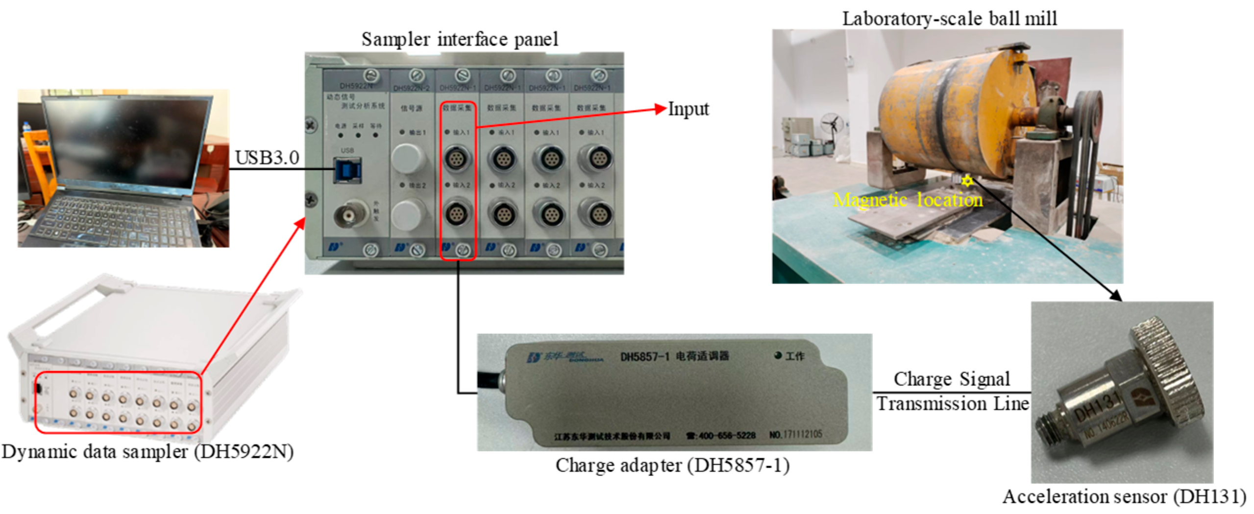
The data acquisition setup for the experimental ball mill is shown in Figure 7a, which mainly consists of three parts: a single ball mill, a dynamic data acquisition instrument (Model: DH5922N, Jiangsu Donghua Test Technology Co., Ltd., Taizhou, Jiangsu, China), and a laptop for real-time monitoring and recording. The acceleration sensor (Model: DH131, Jiangsu Donghua Test Technology Co., Ltd., Jiangsu, China) is installed at the magnetic attachment position (below the ball bearing) as shown in Figure 7b, to collect vibration data transmitted by the ball bearing installed at the bottom of the ball mill. The bearing housing was selected as the measurement point to ensure the acquisition of high-fidelity vibration signals. As a key node for transmitting the internal dynamics of the mill, this location can most comprehensively reflect the overall operating status of the equipment. More importantly, from the perspective of engineering practice, the stable, non-rotating mounting plane provided by the bearing housing is crucial for ensuring the quality and consistency of signal acquisition, and effectively avoids inherent technical challenges such as complex wiring and signal vulnerability to interference when installing sensors on the surface of the rotating cylinder. This strategic selection of measurement points provides a high-quality and high-reliability data source for the model to achieve high-precision classification, serving as the fundamental prerequisite for its optimal performance. The overall schematic diagram of the experimental setup is shown in Figure 8. One end of the dynamic data acquisition instrument is connected to a computing device (a laptop) to ensure accurate and continuous recording of ball mill vibration data; the other end of the acquisition instrument is connected to a charge adapter, which is further linked to the acceleration sensor via a Charge Signal Transmission Line. The sensor is fixed at the designated position in the schematic diagram. The experimental operation procedure strictly follows the working condition scheme in Table 2: First, tungsten ore is fed into the ball mill in accordance with the filling rate and material-ball ratio specified in Table 2, and then the equipment is started. After the equipment operates stably, it is run at a constant speed of 70 r/min (rated speed) and data acquisition is initiated. In this process, the dynamic data acquisition instrument (Model: DH5922N) continuously records vibration signals at a sampling frequency of 20 kHz, with each sample having an acquisition duration of 2 s, to ensure the capture of representative steady-state data. Detailed parameter specifications for the dynamic data acquisition instrument (DH5922N) and the acceleration sensor (DH131) are provided in

Table 3. Technical index of the dynamic data sampler.

Technical Index	Value
Input impedance	10 MΩ//40 PF
Input Method	GND, SIN-DC, DIF-DC, AC, IEPE
Fullness value	±20 mV, ±50 mV, ±100 mV, ±200 mV, ±500 mV, ±1 V, ±2 V, ±5 V, ±10 V, ±20 V
System uncertainty	<0.5% (F.S) (Measurement after half an hour warm-up)
System stability	<0.05%/h (Measurement after half an hour warm-up)
Maximum analysis bandwidth	DC~100 kHz
Operating power	AC power supply	220 V ± 10 V, 50 Hz
	DC power supply	12 V
	Maximum power	150 W

and

Table 4. Technical index of the acceleration sensor.

Technical Index Types	Specific Name	Value
Dynamic indicators	Axial sensitivity	1.23 pC/m·s−2
	Range	5000 m·s−2
	Maximum lateral sensitivity	<5%
	Install resonant frequency	44 kHz
	Insulation resistance	>1010 Ω
	Capacitance	~1300 pF
Environmental parameters	Working temperature range	(−20~120) °C
	Impact limit	10,000 m·s−2
	Base strain sensitivity	0.005 m·s−2/μ ε
	Transient temperature response	0.09 m·s−2/°C
	Electromagnetic sensitivity	40 m·s−2/T

, respectively.

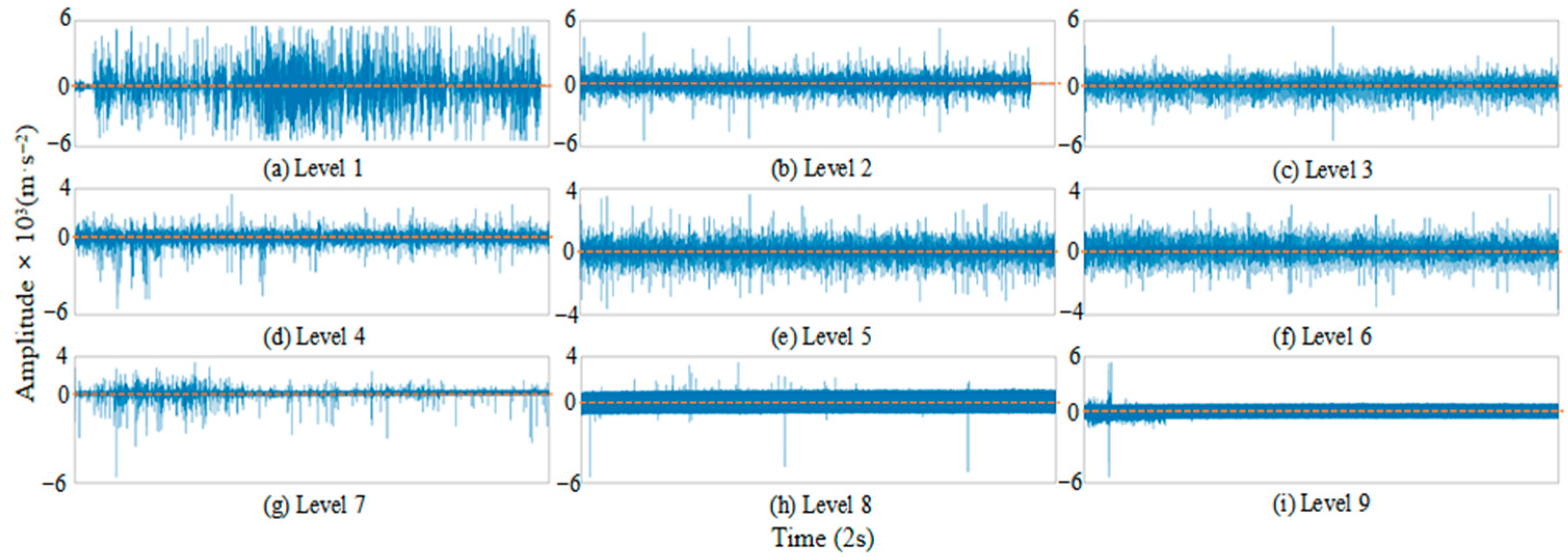
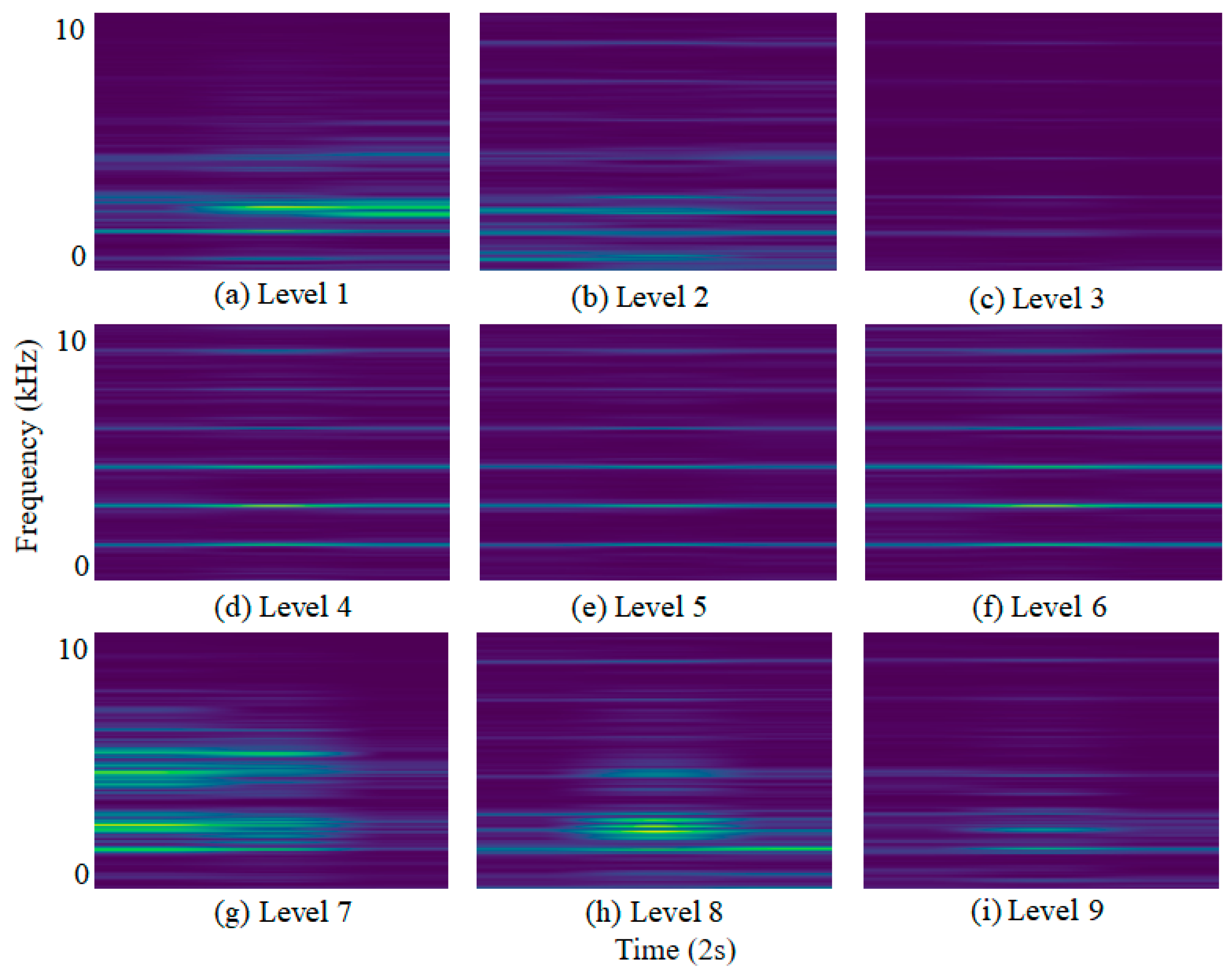
In ball mills, changes in load parameters (such as filling rate and material-to-ball ratio) alter the intensity and frequency of collisions and friction among the “steel balls–materials–cylinder” system inside the mill. This, in turn, leads to characteristic differences in vibration signals across the time domain, frequency domain, and time-frequency domain (STFT time-frequency maps). The two form a direct correlation following the logic of “load determines physical interactions, and physical interactions map to signal features.” Based on this correlation, the characteristic information of the collected vibration signals provides a core basis for ball mill load monitoring. To achieve accurate monitoring, it is first necessary to clarify the load classification criteria. Currently, most scholars classify mill loads into 3 categories [27] (underload, normal load, overload) or 4 categories [28] (no-load impact, underload, normal load, overload) based on the filling rate. However, to characterize the mill’s operating state more clearly, this study classifies mill loads into 9 categories using the filling rate (CVR) and material-to-ball ratio (MBVR). In the experimental setup, the filling rates of 20%, 30% and 40%, and 50% are set to correspond to underload, normal load, and overload states, respectively, with further subdivision based on this. The specific classification criteria are as follows: For the filling rate (CVR): 20% is defined as low filling rate, 30% and 40% as normal filling rate, and 50% as high filling rate. For the material-to-ball ratio (MBVR): 0.1 and 0.3 are defined as low material-to-ball ratio, 0.5 and 0.7 as normal material-to-ball ratio, and 0.9 and 1.1 as high material-to-ball ratio. A total of 9 load levels are obtained through the combination of the above parameters. Figure 9 shows the vibration signals collected from each experimental group; time-frequency maps are generated via Short-Time Fourier Transform (STFT), and the results are presented in Figure 10 (only one time-frequency map is shown for each experimental group).

4.2. Comparative Experiments

Before inputting the one-dimensional vibration signals into each model, it is first necessary to convert them into two-dimensional time-frequency maps through data preprocessing. Specifically, the original time-domain signals are first segmented using a sliding window, where the window width is set to 2048 sampling points and the sliding step is set to 512 sampling points. Subsequently, the Short-Time Fourier Transform (STFT) is applied to each signal segment. According to the analysis in the theoretical section (Section 2.1) of this paper, a Gaussian window is selected as the window function in the transform to achieve the optimal time-frequency resolution, ultimately generating two-dimensional time-frequency images for model input.

To ensure a fair and reproducible comparison, all models were trained under identical experimental conditions, with the key hyperparameter settings detailed in

Table 5. Model Training Hyperparameter Settings.

Hyperparameter Category	Parameter Name	Specific Setting
Training Process	Batch Size	32
	Number of Epochs	200
	Loss Function	Cross-Entropy Loss
Optimizer and Learning Rate	Optimizer	Adam
	Initial Learning Rate	1 × 10−4 (0.0001)
	LR Schedule	ReduceLROnPlateau
Regularization and Early Stopping	L2 Regularization	1 × 10−4
	Dropout Rate	0.5
	Early Stopping	Patience = 15

.

4.2.1. Comparison of Different Methods with STFT Time-Frequency Maps as Input

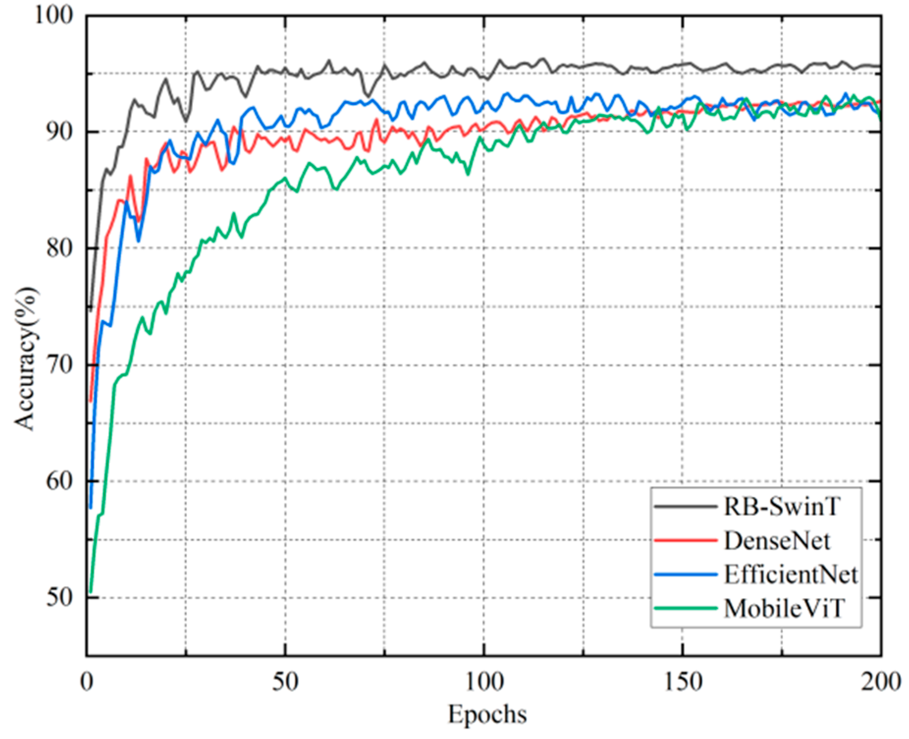
To verify the overall superiority of the model architecture, representative deep learning models such as MobileViT, DenseNet, and EfficientNet were selected as the control group. These models were trained under the condition that the input was also STFT time-frequency maps, with a focus on their convergence stability and classification accuracy.

As shown in Figure 11, the training accuracy curves of all models exhibit a rapid upward trend in the initial training stage, indicating that different models can relatively quickly learn discriminative features from the input data. With the increase in the number of iterations (Epochs), the accuracy curves of each model gradually stabilize. Among them, the training accuracy of the RB-SwinT model not only rises significantly faster than those of DenseNet, EfficientNet, and MobileViT in the initial stage, enabling it to capture key features more quickly, but also stabilizes at approximately 95% in the end, which is at a higher level compared to other models. Although the training accuracies of DenseNet and EfficientNet also gradually stabilize, their rising rates and final convergence accuracies are lower than those of the RB-SwinT model. The training accuracy of the MobileViT model starts relatively slowly, and its final stable accuracy is also lower than that of the RB-SwinT model. The performance of the RB-SwinT model, from rising rapidly to stabilizing first and maintaining high accuracy, fully demonstrates its superiority in feature learning ability and convergence characteristics, laying a foundation for its prominent advantages in subsequent model performance comparison and other analyses.

As shown in Figure 12, the training loss curves of all models show a rapid downward trend in the initial stage, indicating that different models can effectively reduce prediction errors. However, with the increase in the number of iterations (Epochs), the loss curves of MobileViT, EfficientNet, and DenseNet gradually flatten out. In contrast, the RB-SwinT model not only has a significantly faster downward rate in the initial stage but also maintains a certain downward momentum, with the final loss value stabilizing at approximately 0.2, which is at a lower level compared to other models. The loss decline process of the MobileViT model has certain fluctuations, and its final stable loss is higher than that of the RB-SwinT model. Additionally, both the loss decline rates and the final converged loss values of the EfficientNet and DenseNet models are inferior to those of the RB-SwinT model.

These results fully demonstrate the effectiveness of the “global-local collaborative perception” paradigm adopted by the STFT (input) and RB-SwinT network: by synergistically leveraging the global modeling capability of the Swin Transformer and the local refinement capability of the residual module, the network can more efficiently and robustly learn key discriminative features from complex time-frequency maps. This avoids issues such as unstable training or convergence to suboptimal solutions that may occur in other models.

4.2.2. Comparison of Different Methods Under the RB-SwinT Model

Continuous Wavelet Transform (CWT) is a commonly used method in the field of time-frequency analysis. To verify the rationality of using Short-Time Fourier Transform (STFT) as the time-frequency representation front-end, a comparative experiment was designed for ball mill vibration signal processing. The “CWT-RB-SwinT” was adopted as the comparative scheme, and it was jointly applied to the ball mill load recognition task together with “STFT-RB-SwinT”. The time-frequency maps generated by STFT can not only intuitively present the dynamic frequency changes in signals, but also exhibit more stable data distribution characteristics and more convergent training adaptability. This stability can reduce the learning difficulty of machine learning models, decrease fluctuations during the training process, and thereby improve the model training effect. Experimental results show that the RB-SwinT model with STFT time-frequency maps as input has significantly better performance in the ball mill load recognition task than the comparative model with CWT time-frequency maps as input, which fully verifies the rationality of STFT as the time-frequency representation front-end.

As shown in the experimental results in Figure 13, the recognition accuracy of the model based on CWT input is 93.13%, while the model based on STFT input achieves a higher accuracy, which is approximately 3 percentage points higher than the former. This result verifies the hypothesis of this study: the time-frequency maps generated by STFT, which have a more regular structure and more stable patterns, exhibit a higher “learning compatibility” with the RB-SwinT architecture—a vision Transformer based on window and grid division. This compatibility enables the achievement of better performance. This finding provides an important basis for the optimal matching between deep learning models and signal processing front-ends, and highlights the potential advantages of STFT in processing ball mill vibration signals.

4.2.3. Model Classification Accuracy

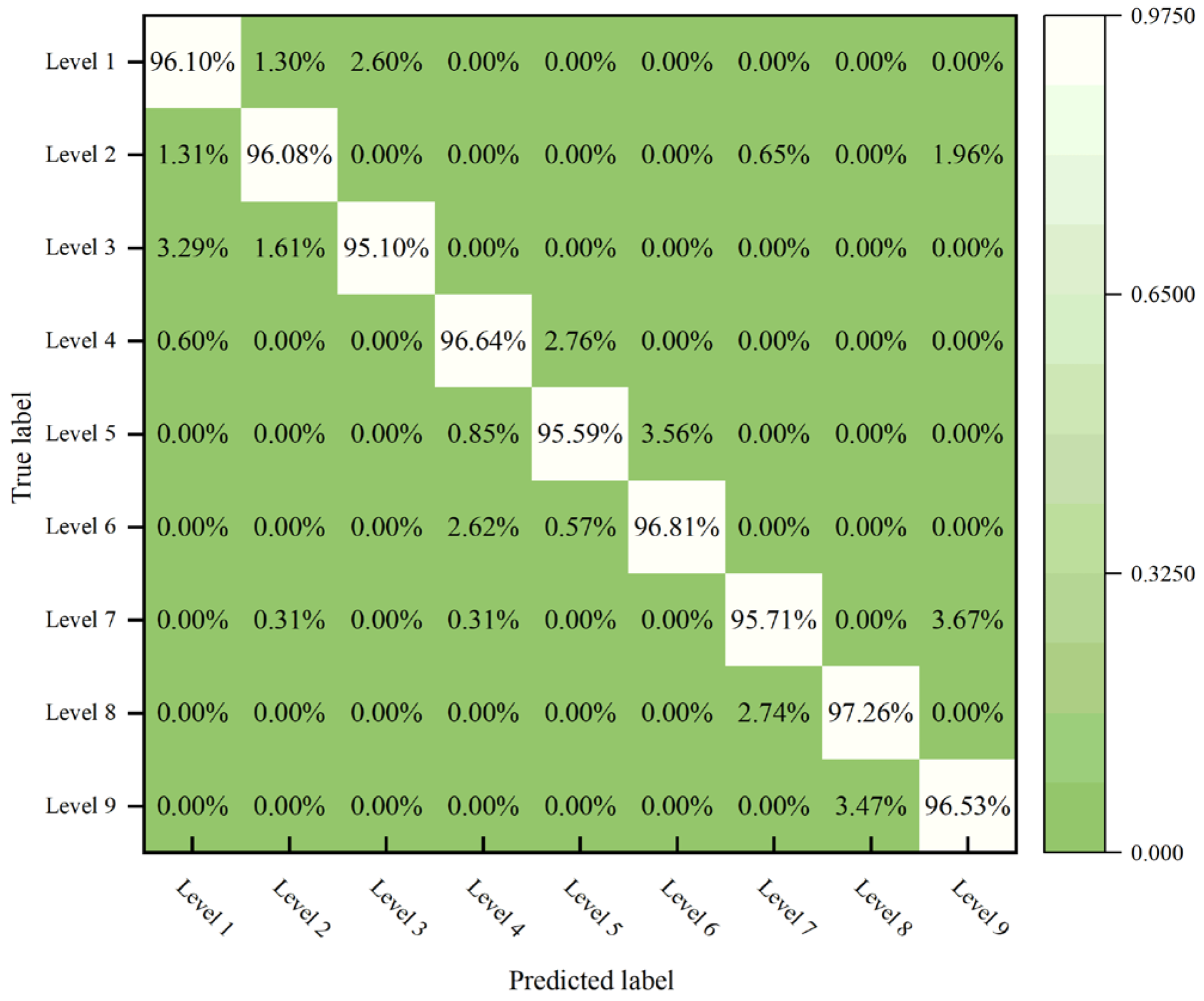
To further quantify the classification performance of the STFT-RB-SwinT model for different load states, a confusion matrix of the model on the test set was generated in this study, as shown in Figure 14. Through a class-by-class visualization format, the confusion matrix presents the model’s prediction results in detail, including specific cases of correct classification and misclassification.

The diagonal elements of the matrix represent the percentage of samples in each category that are correctly classified. It can be clearly seen that the model exhibits excellent recognition performance. For instance, regarding load states such as Level 2, Level 3, Level 6, Level 7, Level 8, and Level 9, the model’s accuracy is close to or even reaches 100%. Even in categories with a small number of misjudgments, the error rate is extremely low. Take Level 1 as an example: 96.10% of the samples are correctly identified, and only 1.30% are misclassified as Level 2—these two are states with relatively similar physical characteristics that are prone to confusion.

Overall, the confusion matrix reveals that the STFT-RB-SwinT model is highly reliable and effective in distinguishing ball mill load states. It intuitively proves that the proposed method can indeed successfully learn highly discriminative deep feature representations from highly entangled original signals, significantly improving the class separability of features.

4.3. Visual Analysis of the Feature Extraction Process

To intuitively verify the feature extraction capability of the STFT-RB-SwinT model, this study used the t-SNE algorithm to perform dimensionality reduction and visualization on the features extracted by the model. t-SNE is a powerful technique that can visualize high-dimensional data into a low-dimensional space while preserving the local neighborhood structure.

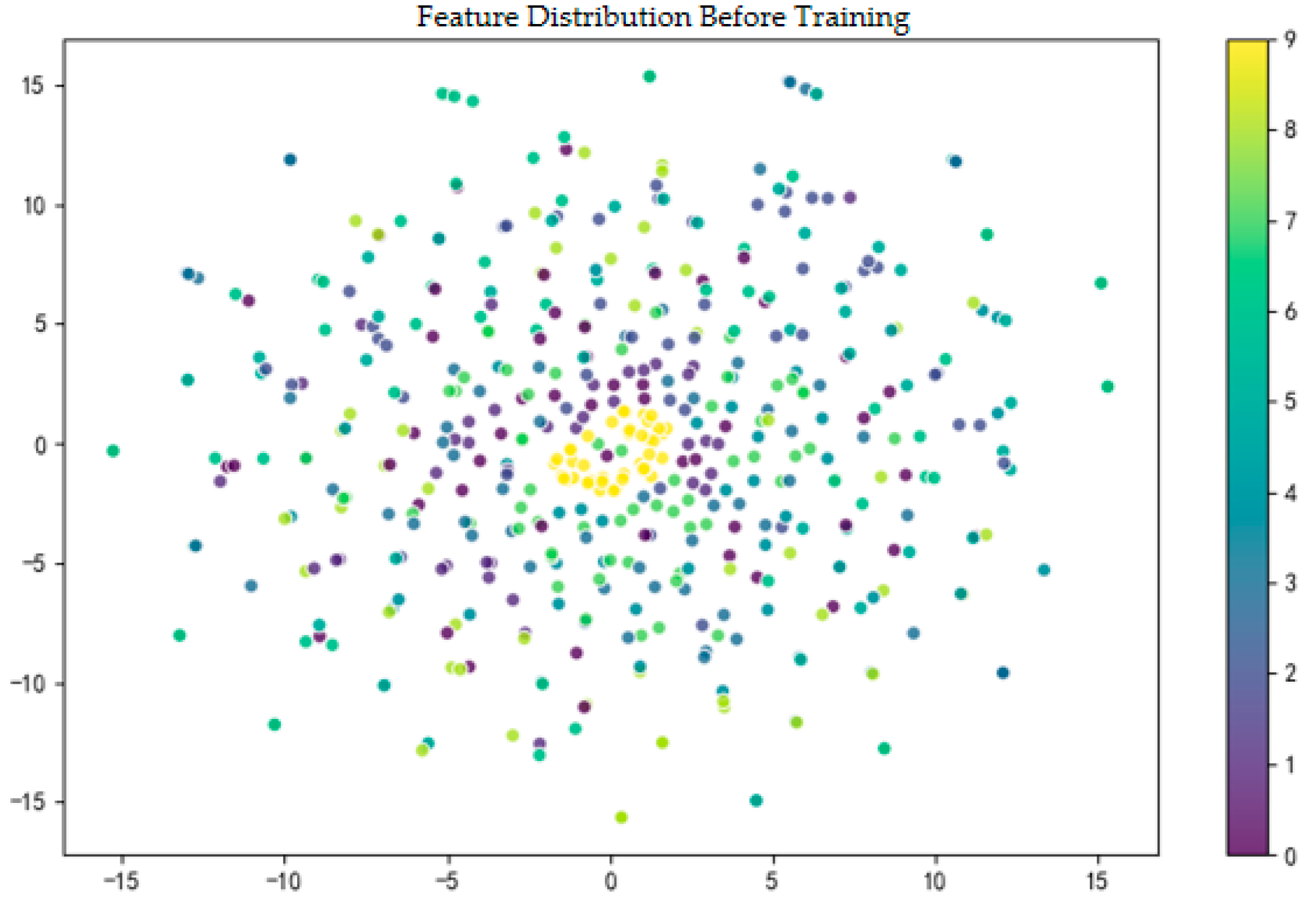
Original Features: As shown in Figure 15, after dimensionality reduction via t-SNE, the original time-frequency features appear as a cluster of highly mixed scatter points in the two-dimensional space. Data points representing 9 different load states (denoted by different colors) are intertwined with each other, lacking any identifiable clustering structure. This intuitively reveals the severe inter-class ambiguity in the original feature space, which originates from the inherent nonlinear and non-stationary characteristics of ball mill vibration signals. This inherent complexity also explains why accurate load identification imposes higher requirements on feature extraction techniques.

Features After Model Processing: In contrast, as shown in Figure 16, the features processed by the proposed RB-SwinT model exhibit a completely different distribution pattern. The feature space is reconstructed into 9 clusters with well-defined boundaries and distinct identities, achieving a remarkable transition from “mixing” to “separability”. This excellent feature separation capability benefits from the model’s unique “global-local cooperative perception” architecture. Specifically, the Swin Transformer backbone network of the model is proficient in capturing the global evolutionary trends and long-range dependencies of signals under different load states; while the innovatively integrated residual module effectively retains and enhances the local transient details that are crucial for classification. It is the synergistic effect of these two components that enables the model to learn a well-structured and highly discriminative feature space from complex original signals, which is the fundamental reason for the model’s excellent classification performance.

4.4. Verification of Model Generalization Ability

The experimental verification in this paper consists of two levels: the first is to verify the model’s targeted performance on the self-built ball mill load dataset, and the second is to evaluate its generalization ability on public benchmark datasets. Previous chapters have completed the verification of the first level; this section will focus on the second level, conducting generalization performance tests on the internationally recognized Case Western Reserve University (CWRU) rolling bearing fault dataset [29].

(1)

Benchmark Dataset and Experimental Settings

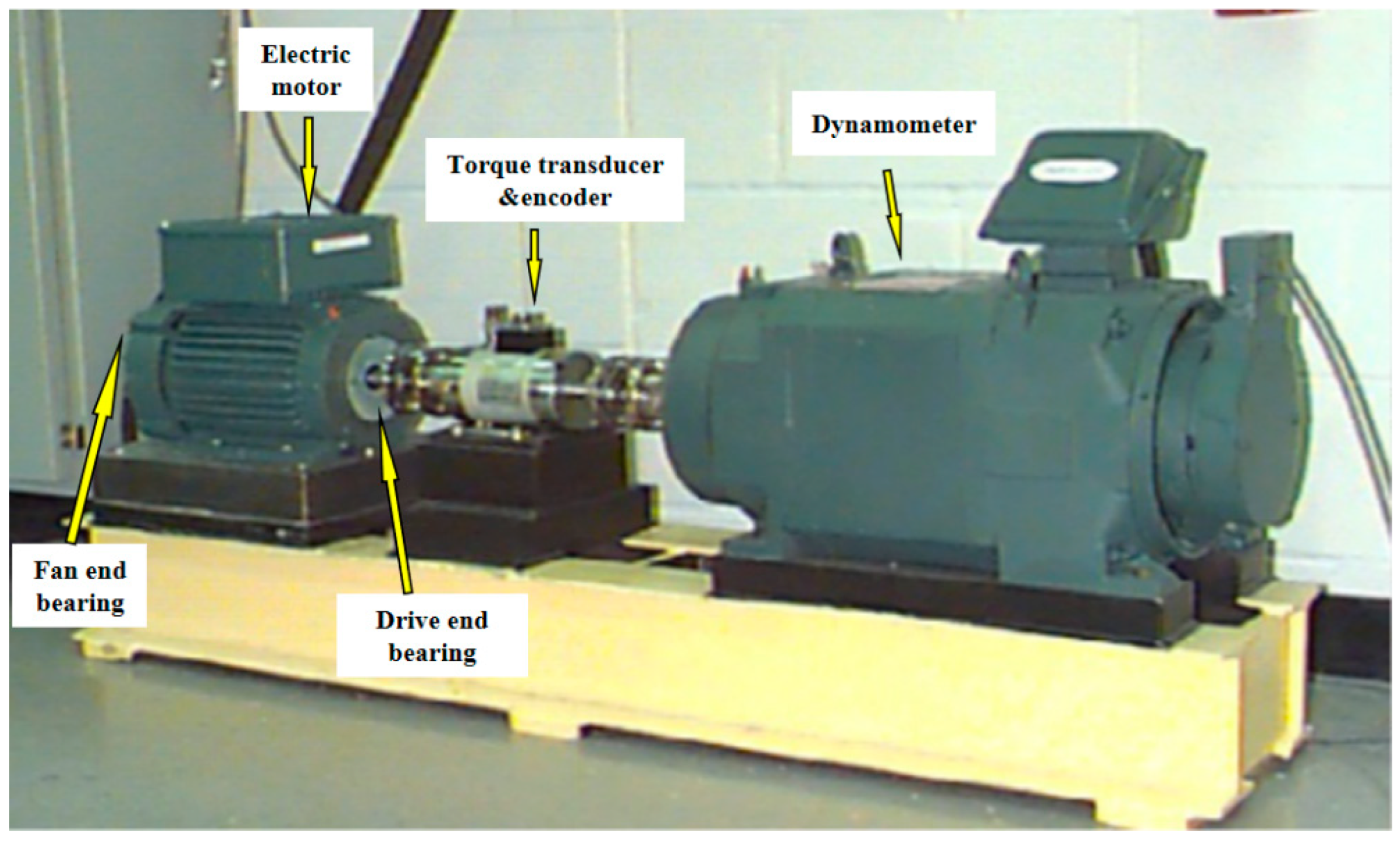
The CWRU dataset is one of the most widely used benchmarks in the field of intelligent diagnosis for rotating machinery, and its experimental platform is shown in Figure 17. Through electrical discharge machining (EDM) technology, the dataset simulates faults of different positions and severities (such as inner race, outer race, and rolling element) on the SKF6205-2RS bearing. Together with the normal state, the dataset includes a total of ten equipment states. Vibration signals were collected by acceleration sensors at a sampling frequency of 12 kHz, and the data contains slight rotational speed fluctuations and environmental noise, providing a realistic test environment for evaluating the model’s robustness.

In the data preprocessing stage, the same sliding window method is adopted, with the window width set to 2048 and the sliding step to 512—that is, 2048 consecutive data points form one sample, the next sample shifts forward by 512 data points, and the overlapping part is 1536. The hyperparameter configuration for model training is consistent with that in the previous experiments, with specific settings shown in Table 5.

(2)

Results and Comparative Analysis

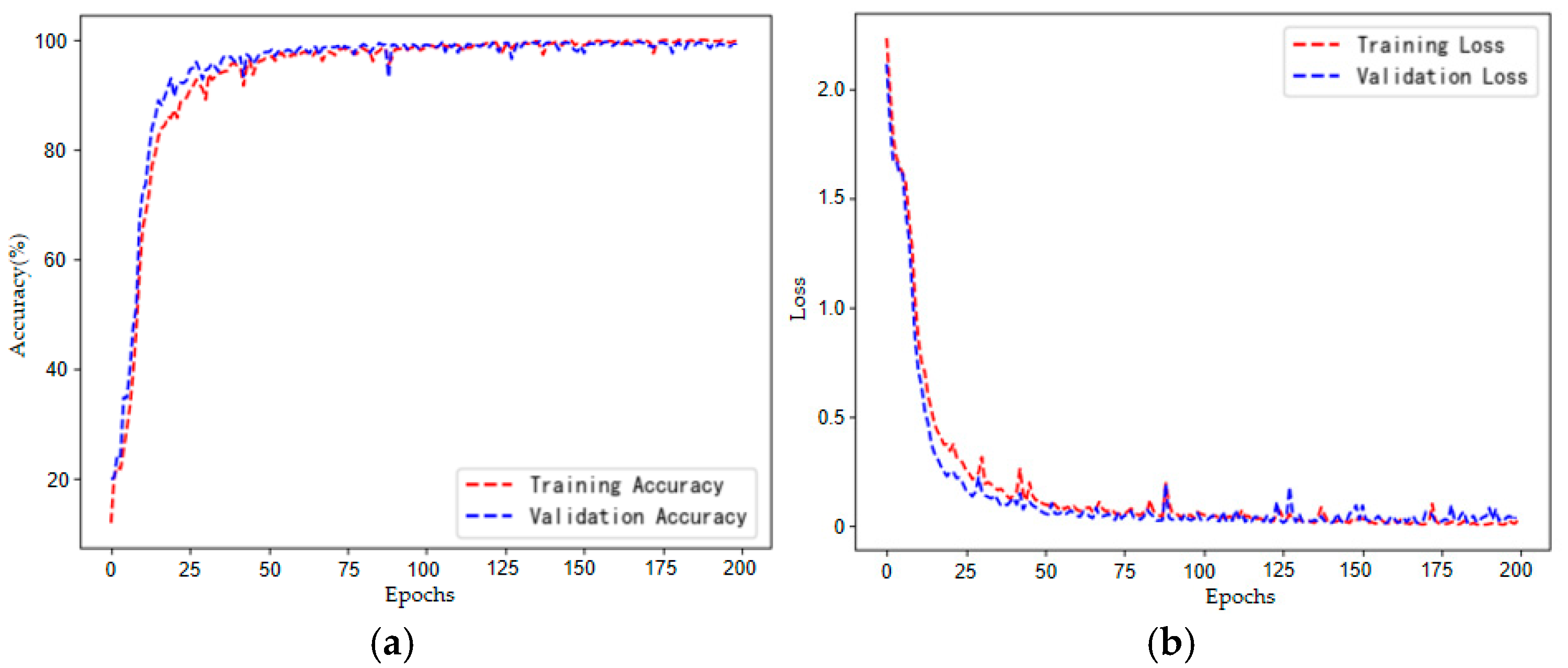
As can be seen from Figure 18, in the initial training stage, the model’s accuracy improves rapidly and the loss value decreases rapidly, indicating that the model can learn efficiently. As training proceeds, both curves stabilize and eventually settle at a level of high accuracy and low loss value. More importantly, the curves of the training set and validation set remain highly consistent throughout the process without significant divergence, which strongly proves that the model has good generalization ability and does not suffer from overfitting. The experimental results show that the RB-SwinT model also performs excellently on this benchmark dataset. After training, the model achieves a final fault identification accuracy of 99.36% on the CWRU test set.

To more objectively position the model’s performance, scholars’ methods including SAVMD-CNN [30], CWT-CNN [31], and ISCNN-LightGBM [32] are selected to compare the fault diagnosis accuracy on the CWRU bearing dataset. The fault identification accuracy of the above methods is shown in

Table 6. Bearing Fault Identification Accuracy of Different Methods.

Method	Comprehensive Accuracy
RB-SwinT (The method proposed in this paper)	99.36%
SAVMD-CNN	98.65%
MTF-CNN	98.91%
ISCNN-LightGBM	99.03%

.

As shown in Table 6, the proposed model in this paper achieves the highest identification accuracy in the comparison, which indicates that its architecture possesses efficient feature extraction ability. To intuitively demonstrate the model’s feature discrimination effect, the t-SNE algorithm is used to perform dimensionality reduction and visualization on the extracted deep features.

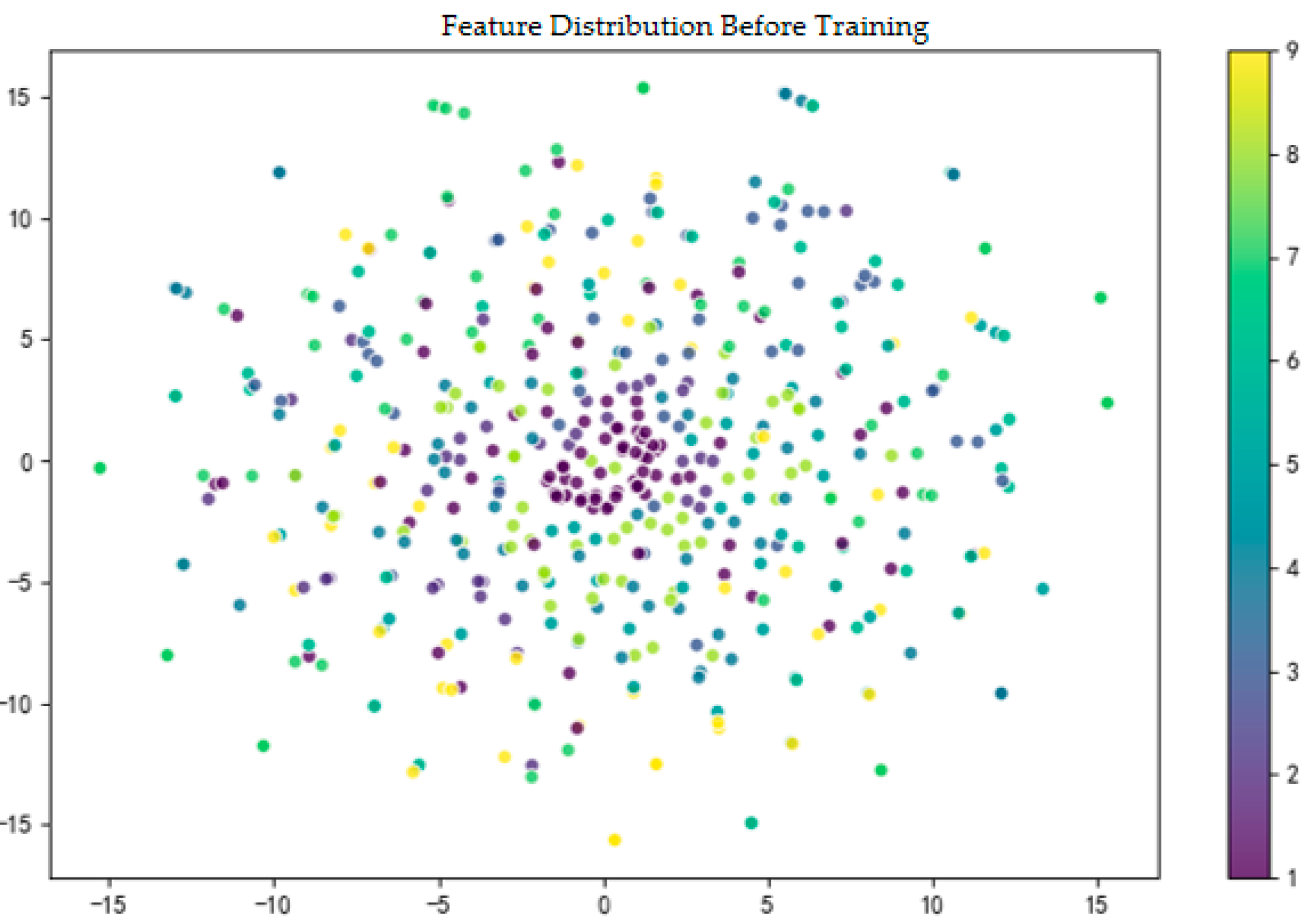
Raw Features: Figure 19 shows the distribution of raw features of 10 different equipment states in the CWRU dataset in the two-dimensional space. As can be clearly seen from the figure, all data points, regardless of their class affiliation (distinguished by color), are highly mixed and clustered together, forming a single, dense central cluster with indistinguishable internal structure. Data points of different classes are intertwined and fail to form any meaningful clusters. This phenomenon intuitively reveals the high coupling and complexity of raw signal features, confirming that it is extremely difficult to directly perform accurate classification of these fault states without effective feature extraction.

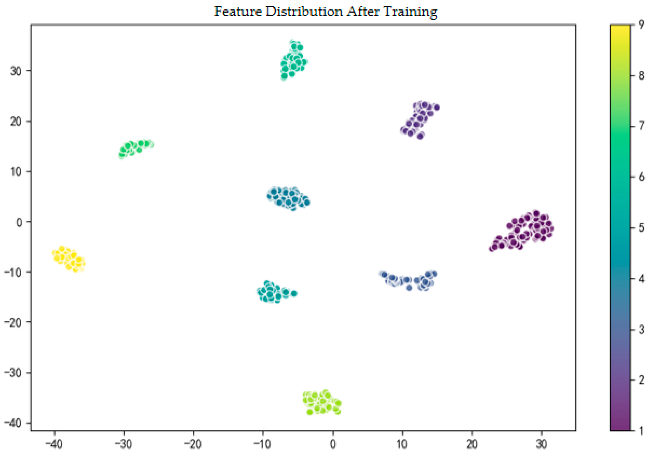
Features After Model Processing: As shown in Figure 20, after deep feature extraction by the proposed RB-SwinT model, the feature space has undergone fundamental reconstruction. The previously mixed data points have been successfully mapped into 10 clusters with clear boundaries and mutual independence. Each cluster exhibits high “cohesiveness” (that is, data points of the same color are closely clustered) and significant “separability” (that is, the distance between clusters of different colors is greatly expanded). This transformation from “chaos” to “order” is a direct visual proof of the model’s good generalization ability. It indicates that the model’s “global-local” collaborative perception paradigm can learn and extract highly discriminative deep feature representations from complex bearing vibration signals, thereby providing an intuitive explanation for the model to achieve effective classification.

5. Discussion

Based on the detailed experimental comparisons in the previous sections, the leading performance of the proposed model in this paper can be clearly confirmed. However, mere numerical advantages are not sufficient to fully reflect its contributions. Therefore, this section will conduct a discussion at a deeper level and objectively examine the challenges and opportunities it faces in its march towards real industrial applications.

5.1. Analysis of the Core Mechanism for Model Effectiveness

The experimental results of this study clearly show that the proposed RB-SwinT model is significantly superior to other mainstream comparative models in classification accuracy, convergence speed, and stability. The root cause of this superiority lies in its unique “global-local collaborative perception” architecture design. The Swin Transformer backbone network successfully captures the long-range dependencies in time-frequency graphs through its efficient shifted window mechanism, which corresponds to the accurate grasp of the macroscopic operating trends of ball mills. Meanwhile, the innovatively integrated Residual Block (ResBlock) plays a key role as a “local detail refiner.” Its shortcut connections provide an information transmission “highway” for high-frequency transient features, effectively avoiding the weakening of key discriminative information in deep networks. It is precisely this complementary design of “the backbone captures trends and residuals preserve details” that enables RB-SwinT to form more comprehensive and robust feature representations than other models.

Compared with other studies in the field, this idea of structural optimization from within the model demonstrates its uniqueness. For example, the method in [33] addresses the receptive field limitations of a single CNN by employing a multi-scale convolutional network (MCNN). Regarding the application of Transformers, researchers have also recognized the performance bottleneck of a single standard Vision Transformer (ViT) model. To address this, some studies such as [34] adopt an external ensemble strategy (fusing diagnostic results of multiple ViT models through soft voting) to improve overall accuracy and generalization ability. Although this ensemble method is effective, it often comes at the cost of increasing the overall complexity and computational cost of the model. In contrast, the RB-SwinT architecture proposed in this study directly enhances the feature expression ability of a single model by cleverly embedding residual blocks within the model. It aims to fundamentally improve the model’s efficiency in capturing dual-scale features in complex industrial signals, providing a new solution for enhancing the intrinsic performance of a single model.

5.2. Rationality of Experimental Design and Characterization of Operating Conditions

The design of this study is intended to thoroughly validate the effectiveness of the “global-local collaborative perception” paradigm under specific conditions (laboratory dry grinding conditions). To this end, an operating condition dataset was constructed, containing 9 fine-grained load variations, which is more demanding for the model’s fine discrimination ability than traditional coarse-grained classification. It is worth emphasizing that the design of this dataset is closely associated with the understanding of operating conditions in industrial practice: a low filling rate of 20% is set to simulate the “underload” operation zone, where Level 1 corresponds to the extreme critical state of “empty grinding”; filling rates ranging from 30% to 40% are set to cover the ideal operating range of “normal load”; and a high filling rate of 50% is set to simulate the “overload” operation zone, where Level 9 corresponds to the critical state of “severe overload”. This design of fine-grained division based on three basic operating conditions aims to ensure that the model can not only distinguish macroscopic states but also capture subtle changes within the states, providing a high-resolution data foundation for achieving accurate process control. Meanwhile, representative mainstream CNN and Transformer variants were selected as comparative models to more comprehensively examine the performance of the proposed RB-SwinT architecture in ball mill load classification.

5.3. Analysis of Limitations and Outlook on Future Work

Although this study has achieved encouraging results, it is equally important to objectively examine its limitations and look ahead to future work.

(1)

Generalizability of Experimental Conditions: The experimental validation of this study was completed on a laboratory-scale dry ball mill. However, in industrial applications, wet grinding conditions are more common. The slurry damping effect introduced by wet grinding may indeed cause changes in the amplitude and high-frequency components of vibration signals. Nevertheless, the “global-local collaborative perception” design philosophy of the proposed model in this paper provides inherent theoretical support for its adaptation to such changes in operating conditions. Firstly, the core of the model lies in learning dynamic “relative patterns” rather than static “absolute features.” The Swin Transformer backbone network learns the “morphological signature” of the entire time-frequency energy distribution, exhibiting good robustness to mere changes in signal amplitude. Secondly, the “global-local collaboration” architecture endows the model with inherent robustness. The integrated Residual Block (ResBlock), acting as a “local detail refiner,” can effectively protect and enhance even weak key discriminative information. Overall, this collaborative learning mechanism for the internal structure and dynamic patterns of signals endows the proposed paradigm with a theoretical basis for adapting to changes in different operating conditions, and provides possibilities for its future application exploration in more complex scenarios such as wet grinding.

(2)

Optimization of Deployment Efficiency: To promote the efficient deployment of the model on resource-constrained industrial edge devices, exploring the lightweighting of the RB-SwinT architecture—such as through techniques like knowledge distillation [35] or network pruning [36]—is also a highly valuable research direction. These subsequent explorations will surely further unlock the potential of the new paradigm proposed in this study.

5.4. Potential Industrial Application Value

From an application perspective, the high-precision load identification method proposed in this study has significant industrial application prospects. Its application value is not limited to providing a classification label, but more importantly lies in the rich process information contained behind the identification results, which can provide an objective reference for on-site operations and process optimization. The accurate identification of the critical state of “severe overload” (Level 9) can provide operators with a clear early warning of choking risk, prompting timely adjustment of the ore feed rate. Similarly, the precise capture of the “empty grinding” (Level 1) state constitutes a serious warning against potential impact wear on the equipment. Furthermore, the high-resolution discrimination ability of this method can capture subtle drifts of operating conditions within the “normal load” zone (such as from Level 5 to Level 4 or Level 6), which provides the possibility for continuous optimization of process parameters and maintaining the equipment at the most efficient operating point. By deploying this model in the grinding production line, accurate determination and monitoring of the ball mill load state can be achieved. This not only liberates operators from the heavy experience-dependent labor but also provides reliable data support for the optimal control of the grinding process. For example, through linkage with control systems, automatic adjustment of the ore feed rate can be realized, enabling the ball mill to operate at the most efficient operating condition at all times. Ultimately, this will offer an effective technical approach for mining enterprises to achieve energy conservation, emission reduction, cost reduction, and efficiency improvement, demonstrating the transformation potential of this research result from theory to practice.

6. Conclusions

In addressing the core challenge in industrial ball mill load state recognition—arising from the nonlinear and non-stationary characteristics of vibration signals—that it is difficult to coordinately model the “global trends” and “local transient features” of signals within a single architecture, this study proposes a novel paradigm based on multi-scale feature collaborative perception. This paradigm is implemented through the residual Swin Transformer network (RB-SwinT) designed in this study. Innovatively, this architecture deeply integrates the powerful global context modeling capability of the Swin Transformer with the excellent local detail refinement capability of the residual block (ResBlock). The experimental results powerfully demonstrate the superiority of our method: on the dataset containing nine categories of fine-grained operating conditions, the overall recognition accuracy of RB-SwinT reaches as high as 96.20%. Additionally, in the generalization ability verification experiment on the public CWRU benchmark dataset, the model also achieves an impressive recognition accuracy of 99.36%, significantly outperforming various mainstream deep learning models while exhibiting faster convergence speed and stronger robustness.

The core contributions of this study extend beyond proposing a high-performance diagnostic model. Theoretically, this work analyzes and resolves the “global-local” feature modeling contradiction prevalent in existing methods. Methodologically, it verifies the feasibility and great potential of successfully transferring the advanced vision Transformer paradigm to industrial process diagnosis. Architecturally, it demonstrates the effectiveness of the RB-SwinT network, whose design philosophy of “the backbone captures trends while residuals preserve details” provides a new and referable approach for similar problems. On this basis, this study further explores the intrinsic correlation between the model’s recognition results and the physical connotation of operating conditions, clarifies the application value of this method in indicating critical states such as “empty grinding” and “overload”, and provides valuable references for the practical application of such methods in the engineering field.

The results of this study have laid a solid technical foundation for realizing the automatic control and energy efficiency optimization of the grinding process, and possess significant theoretical and practical value. Looking ahead, our future work will focus on two directions: first, exploring the lightweight deployment of the model to enable its application in industrial edge computing scenarios with limited computing power; Second, in more complex real industrial environments, conduct verification of the model’s transfer learning and generalization ability under multi-condition and variable-noise scenarios to further promote the practical application of this technology in the real industrial world.

References

1. Gawde, S.; Patil, S.; Kumar, S.; Kamat, P.; Kotecha, K.; Alfarhood, S. Explainable Predictive Maintenance of Rotating Machines Using LIME, SHAP, PDP, ICE. IEEE Access 2024, 12, 29345–29361. [Google Scholar] [CrossRef]
2. Nayak, D.; Das, D.; Behera, S.; Das, S. Monitoring the Fill Level of a Ball Mill Using Vibration Sensing and Artificial Neural Network. Neural Comput. Appl. 2020, 32, 1501–1511. [Google Scholar] [CrossRef]
3. Safa, A.; Aissat, S. Exploring the Effects of a New Lifter Design and Ball Mill Speed on Grinding Performance and Particle Behaviour: A Comparative Analysis. Eng. Technol. J. 2023, 41, 991–1000. [Google Scholar] [CrossRef]
4. Tang, J.; Yu, W.; Chai, T.; Liu, Z.; Zhou, X. Selective Ensemble Modeling Load Parameters of Ball Mill Based on Multi-Scale Frequency Spectral Features and Sphere Criterion. Mech. Syst. Signal Process. 2016, 66–67, 485–504. [Google Scholar] [CrossRef]
5. Xu, H.; Wang, T.; Zou, W.; Zhao, J.; Tao, L.; Zhang, Z. Ball Mill Load Status Identification Method Based on the Convolutional Neural Network, Optimized Support Vector Machine Model, and Intelligent Grinding Media. Chin. J. Eng. 2022, 44, 1821–1831. (In Chinese) [Google Scholar]
6. Qing, Z.; Gao, Y.; Wu, C.; Yang, J.; Wang, Q. Feature Extraction Method of Ball Mill Load Based on the Adaptive Variational Mode Decomposition and the Improved Power Spectrum Analysis. Chin. J. Sci. Instrum. 2020, 41, 234–241. (In Chinese) [Google Scholar]
7. Wu, Z.; Bai, H.; Yan, H.; Zhan, X.; Guo, C.; Jia, X. Intelligent Fault Diagnosis Method for Gearboxes Based on Deep Transfer Learning. Processes 2022, 11, 68. [Google Scholar] [CrossRef]
8. Hermosilla, R.; Valle, C.; Allende, H.; Aguilar, C.; Lucic, E. SAG’s Overload Forecasting Using a CNN Physical Informed Approach. Appl. Sci. 2024, 14, 11686. [Google Scholar] [CrossRef]
9. Cai, G.; Xiao, W.; Xu, H.; Wan, J. Subdivision load identification of ball mill based on multi-domain feature extraction and umap-boxgboost. Signal Image Video Process. 2025, 19, 334. [Google Scholar] [CrossRef]
10. Liu, Y.; Yan, G.; Xiao, S.; Wang, F.; Li, R.; Pang, Y. A multi-task model for mill load parameter prediction using physical information and domain adaptation: Validation with laboratory ball mill. Miner. Eng. 2025, 222, 109148. [Google Scholar] [CrossRef]
11. Huang, P.; Sang, G.; Miao, Q.; Ding, Y.; Jia, M. Soft Measurement of Ball Mill Load Based on Multi-Classifier Ensemble Modelling and Multi-Sensor Fusion With Improved Evidence Combination. Meas. Sci. Technol. 2020, 32, 015105. [Google Scholar] [CrossRef]
12. Luo, X.; Dai, C.; Cheng, T.; Cai, G.; Liu, X.; Liu, J. Load identification method of ball mill based on improved EWT multi-scale entropy and KELM. CIESC J. 2020, 71, 1264–1277. (In Chinese) [Google Scholar]
13. Zhao, J.; Yang, Y.; Lin, X.; Yang, J.; He, L. Looking Wider for Better Adaptive Representation in Few-Shot Learning. In Proceedings of the AAAI Conference on Artificial Intelligence, Palo Alto, CA, USA, 2–9 February 2021. [Google Scholar]
14. Fagbohungbe, O.; Qian, L. The Effect of Batch Normalization on Noise Resistant Property of Deep Learning Models. IEEE Access. 2022, 10, 127728–127741. [Google Scholar] [CrossRef]
15. Li, X.; Wan, S.; Liu, S.; Zhang, Y.; Hong, J.; Wang, D. Bearing Fault Diagnosis Method Based on Attention Mechanism and Multilayer Fusion Network. ISA Trans. 2021, 128, 550–564. [Google Scholar] [CrossRef]
16. Wylomanska, A.; Zimroz, R.; Janczura, J.; Obuchowski, J. Impulsive noise cancellation method for copper ore crusher vibration signals enhancement. IEEE Trans. Ind. Electron. 2016, 63, 5612–5621. [Google Scholar] [CrossRef]
17. Zak, G.; Wylomanska, A.; Zimroz, R. Alpha-stable distribution based methods in the analysis of the crusher vibration signals for fault detection. IFAC-Pap. 2017, 50, 4696–4701. [Google Scholar] [CrossRef]
18. Tanaś, W.; Szczepaniak, J.; Kromulski, J.; Szymanek, M.; Tanaś, J.; Sprawka, M. Modal analysis and acoustic noise characterization of a grain crusher. Ann. Agr. Environ. Med. 2018, 25, 433–436. [Google Scholar] [CrossRef] [PubMed]
19. Liu, Z.; Lin, Y.; Cao, Y.; Hu, H.; Wei, Y.; Zhang, Z.; Lin, S.; Guo, B. Swin transformer: Hierarchical vision transformer using shifted windows. arXiv 2021, arXiv:2103.14030. [Google Scholar] [CrossRef]
20. Li, H.; Zhang, Q.; Qin, X.; Sun, Y. Fault diagnosis method for rolling bearings based on short-time Fourier transform and convolution neural network. J. Vib. Shock 2018, 37, 124–131. (In Chinese) [Google Scholar]
21. He, K.; Zhang, X.; Ren, S.; Sun, J. Deep residual learning for image recognition. In Proceedings of the IEEE Conference on Computer Vision and Pattern Recognition (CVPR), Las Vegas, NA, USA, 26 June–1 July 2016. [Google Scholar]
22. Wang, R.; An, S.; Liu, W.; Li, L. Invertible residual blocks in deep learning networks. IEEE Trans. Neural Netw. Learn. Syst. 2024, 35, 10167–10173. [Google Scholar] [CrossRef]
23. Tang, J.; Chai, T.Y.; Liu, Z.; Yu, W. Selective ensemble modeling based on nonlinear frequency spectral feature extraction for predicting load parameter in ball mills. Chin. J. Chem. Eng. 2015, 23, 2020–2028. [Google Scholar] [CrossRef]
24. Kim, Y.; Kim, Y. Time-frequency multi-domain 1D convolutional neural network with channel-spatial attention for noise-robust bearing fault diagnosis. Sensors 2023, 23, 9311. [Google Scholar] [CrossRef]
25. Wu, J.; Luo, W.; Yao, K. Electric motor vibration signal classification using Wigner-Ville distribution for fault diagnosis. Sensors 2025, 25, 1196. [Google Scholar] [CrossRef]
26. Yu, H.; Wang, X.; Li, J.; Xue, Y.; Zou, S.; Liu, J. Study on the relationship between grinding medium particle size and ball mill grinding efficiency. Min. Mach. 2020, 48, 32–37. (In Chinese) [Google Scholar]
27. Yang, L.; Yang, H. Load identification method of ball mill based on the CEEMDAN-wavelet threshold-PMMFE. Gospod. Surowcami Miner. 2024, 40, 163–180. [Google Scholar] [CrossRef]
28. Cai, G.; Liu, X.; Dai, C.; Luo, X. Load state identification method for ball mills based on improved EWT, multiscale fuzzy entropy and AEPSOPNN classification. Processes 2019, 7, 725. [Google Scholar] [CrossRef]
29. Smith, W.; Randall, R. Rolling Element Bearing Diagnostics Using the Case Western Reserve University Data: A Benchmark Study. Mech. Syst. Signal Process. 2015, 64–65, 100–131. [Google Scholar] [CrossRef]
30. Song, C.; Liang, Y.; Lu, N.; Du, G.; Jia, B. Bearing Fault Diagnosis Method Based on SAVMD and CNN. J. Mech. Strength 2024, 46, 509–517. (In Chinese) [Google Scholar]
31. Lei, C.; Xia, B.; Xue, L.; Jiao, M.; Zhang, H. Rolling Bearing Fault Diagnosis Method Based on MTF-CNN. J. Vib. Shock 2022, 41, 151–158. (In Chinese) [Google Scholar]
32. Zhang, S.; Ji, H.; Liu, Y. Bearing Fault Diagnosis Based on ISCNN-LightGBM. Control Theory Appl. 2023, 40, 753–760. (In Chinese) [Google Scholar]
33. Lv, D.; Wang, H.; Che, C. Multiscale Convolutional Neural Network and Decision Fusion for Rolling Bearing Fault Diagnosis. Ind. Lubr. Tribol. 2021, 73, 516–522. [Google Scholar] [CrossRef]
34. Tang, X.; Xu, Z.; Wang, Z. A Novel Fault Diagnosis Method of Rolling Bearing Based on Integrated Vision Transformer Model. Sensors 2022, 22, 3878. [Google Scholar] [CrossRef]
35. Wang, Y.; Yang, S. A Lightweight Method for Graph Neural Networks Based on Knowledge Distillation and Graph Contrastive Learning. Appl. Sci. 2024, 14, 4805. [Google Scholar] [CrossRef]
36. Shah, S.; Berahas, A.; Bollapragada, R. Adaptive Consensus: A Network Pruning Approach for Decentralized Optimization. SIAM J. Optimiz. 2024, 34, 3653–3680. [Google Scholar] [CrossRef]
Figure 1. General residual block structure.
Machines 13 01045 g001
Figure 2. The hierarchical structure of Swin Transformer.
Machines 13 01045 g002
Figure 3. Schematic diagram of shifted windows.
Machines 13 01045 g003
Figure 4. Traditional Swin Transformer model structure. (a) Architecture; (b) Two Successive Swin Transformer Blocks.
Machines 13 01045 g004
Figure 5. Stage schematic of SwinT with residual module. (a) One stage of Swin Transformer; (b) Architecture of ResBlock.
Machines 13 01045 g005
Figure 6. Schematic structure of the model based on STFT and RB-SwinT.
Machines 13 01045 g006
Figure 7. Laboratory-scale ball mill layout. (a) Experimental equipment; (b) Laboratory-scale ball mill.
Machines 13 01045 g007
Figure 8. Experimental connection diagram.
Machines 13 01045 g008
Figure 9. The vibration signal for each experiment.
Machines 13 01045 g009
Figure 10. STFT time-frequency graphs for each experiment.
Machines 13 01045 g010
Figure 11. Comprehensive Performance Comparison (Accuracy) Between STFT-RB-SwinT and Mainstream Methods.
Machines 13 01045 g011
Figure 12. Comprehensive Performance Comparison (Loss Value) Between STFT-RB-SwinT and Mainstream Methods.
Machines 13 01045 g012
Figure 13. Comparison of STFT and CWT time-frequency graphs as input training results.
Machines 13 01045 g013
Figure 14. Confusion matrix prediction schematic.
Machines 13 01045 g014
Figure 15. Visualization of Features Before Extraction by the Model.
Machines 13 01045 g015
Figure 16. Dimensionality Reduction Visualization of Features After Extraction by the Model.
Machines 13 01045 g016
Figure 17. Case Western Reserve University (CWRU) Rolling Bearing Fault Experimental Platform.
Machines 13 01045 g017
Figure 18. Training Iteration Status Based on the CWRU Dataset. (a) Accuracy Curve; (b) Loss Value Curve.
Machines 13 01045 g018
Figure 19. Visualization of Pre-Extraction Features of the RB-SwinT Model on the CWRU Dataset.
Machines 13 01045 g019
Figure 20. Visualization of Post-Extraction Features of the RB-SwinT Model on the CWRU Dataset.
Machines 13 01045 g020