Abstract
In this paper, the rail mean vertical alignment is estimated through double integration of wheel–rail contact forces measured using dynamometric wheelsets on a dedicated track recording vehicle (TRV). A simplified three degrees of freedom (DOF) linear model of half a train coach has been developed for this purpose. The model’s ability to simulate the average left and right longitudinal level has been tested using vertical contact force recordings from a constant speed track section, as measured by the TRV. The results are compared with available track geometry (TG) data, recorded by the optical system of the same vehicle, used for condition monitoring of the Italian railway infrastructure. Model parameters, such as masses, stiffness, and damping of the suspensive system have been optimized. An error analysis has been conducted on results. A good agreement is found between simulated and recorded vertical alignment at the D1 level, suggesting the feasibility of using contact forces measured with instrumented wheelsets for railway TG condition monitoring. This computationally efficient approach highlights the potential of strain gauges and instrumented wheelsets as alternative or complementary technologies to the widely adopted accelerometers, rate gyros, and optical devices for railway condition monitoring. Given its low computational cost, embedded and real-time TG estimation could be further investigated.
1. Introduction
Rail transportation in Europe accounts for a significant share of total passenger and freight transport (11.9% in 2022) [1], with rapid growth following the COVID-19 pandemic. Ensuring fast, safe, and comfortable journeys is key to increasing rail transport’s market share against competitors such as cars, trucks, buses, air, and maritime transport. The condition of railway tracks is critical for the safe and efficient operation of mass passenger and freight transport. Track degradation is a primary cause of service disruptions, delays, and accidents, often linked to derailments or un-scheduled maintenance. To ensure rail travel remains fast, safe, and comfortable, aligning with Sustainable Development Goal (SDG) 9, “Industry, Innovation, and Infrastructure”, continuous monitoring and inspection of railway infrastructure are essential. This enables predictive maintenance by assessing real-time conditions and tracking the deterioration trends of railway components. Proper assessment of rail integrity relies on well-defined condition indices, facilitating the adoption of new predictive maintenance strategies. It is crucial to measure physical quantities that directly or indirectly indicate infrastructure degradation. The measurement of wheelrail contact forces and axle boxes, bogies, and car bodies accelerations onboard railway vehicles plays a fundamental role in this process. A growing trend in the railway sector involves continuous monitoring of infrastructure using sensors installed both on vehicles and trackside. This approach enables condition-based maintenance, triggered when track degradation reaches non-negligible levels. Key parameters, such as the catenary, superstructure, and track foundation, can be monitored using onboard sensors [2] typically installed on dedicated track recording vehicles (TRVs). These vehicles facilitate long-range rail inspections, allowing many simultaneous measurements such as pantograph–catenary interaction, wheel–rail interaction, and track geometry (TG) [3]. Other inspection methodologies, involving the use of portable trolleys, are costly and time consuming, requiring track occupation for extended periods and the involvement of highly specialized workers and technicians. In the Italian railway infrastructure, each type of railway line is regularly inspected by different TVRs equipped with dedicated sensors. Commonly adopted technologies include inertial sensors (accelerometers, rate gyros), video inspection and contactless systems (laser scanners, cameras), force/strain measurement devices (strain gauges, load cells), as well as eddy current and ultrasound sensors [3,4]. Although instrumented wheelsets (IWS) are installed onboard, their use is typically limited to running dynamics assessment rather than TG monitoring for their relatively higher cost. Given their direct contact with the rail, without the interposition of a suspension system to mitigate interactions, contact forces measured by these devices can provide valuable insights into rail conditions, including both running surface integrity and TG anomalies. They are primarily employed to evaluate maximum allowable contact forces and to monitor the derailment index (Y/Q ratio), particularly in freight operations. To the author’s knowledge, academic research on the use of IWS for railway infrastructure condition monitoring is scarce. While numerous studies focus on optimal strain gauge positioning, layout optimization, and finite element (FE) modelling for assessing strain states for inverse force identification or frequency responses, very few explore the potential of IWS for direct track condition monitoring [5,6,7].
The paper is structured as follows. The state-of-the-art review of TVRs and in-service vehicle technologies for railway condition monitoring is presented in Section 2 and Section 3. A detailed description of the 3-DOF lumped model used in this paper is presented in Section 4. Results discussion and error analysis are presented in Section 5 and Section 6, respectively. Conclusions and future research perspectives are given in Section 7. The whole work is an extended version of a previous conference paper [8] in which the proposed estimation method has been introduced for the first time in a much simpler way.
2. State-of-the-Art Review of Equipment and Methods for Railway Condition Monitoring
A significant portion of academic research in railway condition monitoring focuses on kinematic and inertial measurement. Vibrations and kinematics of specific vehicle components such as car bodies, bogies, or axle boxes are recorded as specified by the European standards EN 13848-1 and EN 14363 [9,10]. These measurements are used to assess TG quality, which includes parameters such as track gauge, lateral alignment, longitudinal level (also referred to as vertical alignment or top), twist and superelevation (also known as cant or cross-level). These parameters are typically analyzed within specific wavelength ranges (D1, D2, and D3), as defined by the standards and summarized in Table 1.

Table 1.
EN 13848–1 standardized wavelength ranges.
In onboard monitoring systems, TG is either measured directly or estimated using redundant inertial or optical sensors. Displacements are typically derived from acceleration data through direct integration or by combining angular velocities with other TG parameters, such as horizontal curvature for cross-level estimation [11,12], or vertical and lateral alignment assessment [13,14]. For these applications, accelerometers and rate gyros are the most common sensors. Additionally, other technologies, such as inertial and chord-based laser scanners, measure optical displacements from the rail centreline, generating high-resolution point cloud mappings of the track [15,16]. A schematic representation of available sensors mounted on the RFI’s Diamante TRV [17] for inspection of high-speed lines is shown in Figure 1.
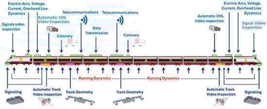
Figure 1.
Schematic representation of available sensors mounted on the RFI’s Diamante TRV for high-speed lines diagnosis [17].
The ability to estimate track geometry parameters, including alignment, longitudinal level, and cross level, makes these sensors and systems well suited for railway infrastructure condition monitoring. Parsing maximum lateral and vertical accelerations makes possible assessing ride comfort of train journeys. Furthermore, it serves for the static homologation of vehicles and components under specific testing conditions. Despite this, accurately estimating wheel–rail contact forces using only accelerometers remains a challenge for onboard monitoring. In contrast, IWS provides an alternative method for force estimation. These wheelsets employ strain gauges to measure the deformation of structural components, providing a reliable method for an inverse measurement of wheel–rail contact forces. When properly installed on a component’s surface, strain gauges generate an electrical signal proportional to the experienced strain [17,18,19,20,21,22]. Also referred to as dynamometric wheelsets, IWS is primarily used for specialized applications, such as testing and homologation of vehicles and components. However, the application in condition monitoring remains limited, mainly due to high costs, complex installation procedures, and the need for highly specialized labour. Despite these challenges, they provide high-precision contact force estimations and are considered an established technology for this purpose [23].
Wear of railway components has a significant impact on exchanged contact forces. Contact conditions vary considerably depending on the shape of the worn wheel and rail profiles, determined by the amount of wear, which in turn affects the overall ride quality [24,25,26]. A comprehensive review of green tribology and wear evaluation methods is presented in [27,28], highlighting techniques to quantify wear in engineering surfaces under operational conditions with valuable examples for the maintenance of wheels and rails. However, in the present study, the analysis focuses on a relatively precise bandwidth of measured contact forces, filtered within the selected range and used to derive a reliable estimation of the rail’s vertical alignment.
Even under strict measurement standards, small estimation errors can arise during test campaigns [29]. Given the various sources of error and uncertainty in real-world applications, even minor uncertainties in the measurement chain can introduce small offsets and drifts, resulting in non-zero mean terms. These terms become problematic when double integrating acceleration data to obtain displacements, as they amplify errors throughout the integration process. If a measurement contains spurious terms or offsets, often introduced during sensor calibration or taring, non-zero mean terms emerge in the time-series data. While these small errors may seem negligible in direct comparisons, their impact grows significantly when integrated over time, leading to deviations from the expected physical behaviour of the system. Thus, estimated quantities may exhibit unrealistic or even diverging displacements, inconsistent with the physical model or observed system behaviour. Moreover, integrating noise causes the root mean square (RMS) value of the output to increase over time, even when no actual changes occur in the sensor’s state (e.g., motion in accelerometers or strain in strain gauges) [11]. On the other hand, in theory, integrating measured data can yield displacements and positions; in practice, this process is often compromised by such errors. A common solution is the application of high-pass filters to mitigate drifts and stabilize the integration of acceleration data derived from measured forces [12]. Offset identification and compensation in real-world measurements are often performed using direct and indirect Kalman filtering [30]. However, these filters require a well-defined model of the sensing process, along with knowledge of the covariance matrix and the errors associated with the acquisition instrumentation. In this study, a second order Butterworth high-pass filter has been applied as a pre-processing step to the acquired data, along with the use of a simplified system model. This model could potentially serve as a foundation for the future development of a Kalman filter. For the current work, the focus is on applying a time-domain filter and a simplified model to estimate equivalent displacements, and thereby detect track defects, within the wavelength range specified by the standards. These wavelengths align with the domain of validity of the proposed model.
3. Review of Models and Methods for On-Board Railway Condition Monitoring
Lewis and Richards [12] proposed a method for estimating track cross-level using a reduced sensor set. They combined high-frequency vibration data from horizontally oriented accelerometers with low-frequency data from a rate gyro. Using a carefully selected crossover frequency, they employed a third-pole Butterworth filter to reconstruct rail superelevation from onboard measurements.
Weston et al. [13,14] developed methods for estimating mean vertical and lateral track alignment using sensors mounted on in-service vehicle bogies. Their approach relied on bogie-mounted vertical and lateral accelerometers, along with yaw rate sensors, to estimate mean lateral track irregularities without requiring optical or contact sensors. They demonstrated that a yaw rate gyro can serve as an alternative to a roll-compensated lateral accelerometer. Additionally, they introduced an inverse model based on a Kalman filter to improve estimation accuracy at specific vehicle speeds. Their method treated lateral track irregularities as an integrated random walk, with yaw rate serving as the system’s observation input.
Sun and Dhanasekar [31], and Zhai and Cai [32], developed a dynamic railway vehicle model to examine vertical interactions between the track and waggon system and for simulating train–track interaction at the wheel–rail interface. Their 10-DOF lumped mass system consists of a carbody, two bogies (including the respective inertial properties), and four unsprung wheelset masses. The track is modelled as an infinitely long beam discretely supported at rail–sleeper junctions, with the contact patch represented by Hertzian contact. Using this model, they investigated the track’s dynamic response at rail joints and quantified the relationship between unsprung mass and dynamic wheel–rail forces.
Kawasaki and Youcef-Toumi [33] developed an inverse model for estimating vertical, lateral, and cross-level track irregularities using carbody acceleration measurements. Their approach was validated with data collected onboard a Shinkansen train. While vertical and lateral irregularities were accurately estimated, level irregularities exhibited more bias compared to reference data. The authors highlighted that vehicle mass and speed significantly influence estimation accuracy, requiring different model parameters to accommodate variations.
Mori et al. [34] developed a portable track condition monitoring system for high-speed railways. The detection and identification of rail irregularities from in-service vehicles uses acceleration data and carbody roll angle. Rail corrugation is detected using cabin noise and spectral peak calculation. The location of identified faults is pinpointed along the track by a GPS and a map-matching algorithm. Filed tests were conducted to determine the performance of the equipment and method.
Odashima et al. [35] proposed a track condition monitoring technique using carbody acceleration measured by in-service vehicles. Authors demonstrated that estimating track irregularities of conventional railway tracks using carbody acceleration only is possible with a bias between experimental TVR data and estimated by the model of 1 mm. Their method uses inverse dynamics by applying a Kalman filter. For the latter, track geometry is expressed in a random walk model, incorporating it into a state equation. Impulse response is incorporated as measurement equation supporting variations in vehicle speed.
Alfi and Bruni [36] proposed a method for estimating long wavelength track irregularities using vehicle acceleration measurements and a 6-DOF model comprising three rigid bodies: the carbody and two bogies. Each body was assigned two degrees of freedom, accounting for vertical displacement and pitch rotation, while all other motions were neglected. The model assumed that the wheels followed track irregularities without separation and that the vehicle moved at a constant forward speed. Acceleration data were processed using a frequency domain model-based identification procedure, decomposing track irregularities into harmonic components that were identified separately. The method was validated and compared with measurements from a track recording vehicle (TRV) on high-speed lines.
Miwa et al. [37] investigated the influence of mass variation on dynamic wheel–rail load fluctuations through numerical simulations and test rig experiments. Their findings showed that unsprung mass has the most significant impact on wheel dynamic load variations. Reducing wheel mass effectively decreases the acting load, particularly at higher vehicle speeds. In contrast, variations in sprung masses (bogies and carbody) had only a minor influence on dynamic load variations.
Recent research has focused on machine learning (ML) and data-driven methods for railway condition monitoring. Both supervised and unsupervised anomaly detection algorithms, enable rapid processing of large datasets. These methods uncover hidden relationships between input features and key track parameters, even when traditional analytical relationships are difficult to establish. Typically, they classify track sections into “anomalous” or “healthy” categories, making them particularly useful for detecting faults in large railway networks.
Tsunashima [38] implemented a track condition monitoring system using an onboard sensing device and machine learning techniques to diagnose track conditions based on carbody vibrations. The equipment and method were used to automatically detect and classify track irregularities on regional railway lines in Japan.
La Paglia et al. [39] developed a condition monitoring system based on bogie acceleration measurements from in-service high-speed trains. Using prebuilt multiple regression models, the system estimated track longitudinal level. Synthetic indicators, such as the root mean square (RMS) of bogie vertical acceleration, were computed and correlated with the maximum rail top level. This methodology distinguished between isolated and distributed defects and tracked vertical alignment evolution over time.
De Rosa et al. [40] introduced an ML-based classifier for monitoring lateral and cross-level track irregularities using lateral and roll bogie frame accelerations. The classifier was trained on synthetic data and validated using real measurements from a diagnostic vehicle operating at 300 km/h on a straight high-speed rail line. Three ML algorithms were tested: linear support vector machine (LSVM), Gaussian support vector machine (GSVM), and decision tree (DT). While all performed well, GSVM yielded the highest accuracy for identifying lateral track faults, whereas DT had the lowest performance.
Ghiasi et al. [41] proposed an artificial intelligence (AI)-based framework for TG diagnosis using acceleration data from bogies and carbody of a dedicated high-speed TRV. The anomaly detection system involved two stages: feature selection and a data-driven anomaly detection algorithm based on the one-class support vector machine (OCSVM). The study compared OCSVM against isolation forest (IF), local outlier factor (LOF), and robust Mahalanobis distance (RMD) and found that OCSVM provided the highest detection accuracy, outperforming approaches that relied on raw acceleration data alone.
Gullers et al. [42] developed a track condition analyser (TCA) based on ML techniques and instrumented wheelset force measurements. The system classified track conditions using supervised learning and labelled datasets of faulty and healthy track force recordings. It identified short-pitch rail corrugation, rolling surface defects with isolated or periodic force transients, and stiff rail supports. Characteristic features, including mean values, percentiles, and standard deviations of vertical contact forces (Q), were extracted and filtered across different frequency intervals. To the authors’ knowledge, this study represents one of the first applications of IWS and force recordings for rail superstructure condition monitoring.
This paper presents a model-based method that utilizes wheel–rail contact forces measured with IWS and a simplified 3-DOF train coach system to estimate the mean vertical rail longitudinal level within the D1 wavelength range. The model was tested using experimental data from a dedicated TRV and validated across a speed range of 100 km/h to 200 km/h, making it applicable to most conventional railway lines. One key advantage of this approach is its ability to rapidly process several minutes of recorded data, making it suitable for embedded real-time and online applications. However, further research is needed to improve estimation accuracy and extend the model’s applicability to non-constant speed track sections. The use of contact force recordings for track geometry condition monitoring is a promising development in railway maintenance. This study highlights the potential for expanding the role of IWS beyond their traditional applications.
4. Instrumented Wheelsets and Data Acquisition
All input data for the model, specifically excitation vertical forces and reference track geometry data (longitudinal level) were recorded by a dedicated TRV used for Italian railway tracks and whole infrastructure condition monitoring. Due to NDA, these datasets are protected and not publicly available. Other limitations concerning the type of TRV used, equipment for data recording and storage, are all limited and not available. In particular, the instrumented wheelset strain gauges layout is strictly protected, but some reference of specific application for inverse force identification in the railway sector can be found in the literature (Gomez et al. [5], Bellacci et al. [19], Ronasi et al. [20]). Usually, for this kind of applications, sensors are installed on both the inner and the outer surface of the wheel-web and on the axle. This allows a finer and more precise estimation of the vertical and lateral contact forces by applying a calibration matrix to the recorded data, as reported in Bellacci et al. [19] and Diana et al. [43], adding the possibility to estimate the contact patch position area [44]. Data can be transmitted from the rotor (wheels) to the stator (carbody), by an antenna (static antenna), which powers the strain gauges’ Wheatstone bridges, filters, and converts the digitalised signal received from the rotor antenna into analogue. The rotor antenna instead amplifies and digitalises the acquired data before sending them to the static antenna. Studies on equipment’s frequency response and passband were previously conducted, although with severe limitation on the impact test hammer, which was introducing strong noise to the measurements [22].
Some simplified schematic examples of strain gauges layouts mounted on the wheel web are shown in Figure 2. Since the wheel is rotating, multiple quadrature bridges can be installed. Other frequently used configurations are called “distributed” bridges with equally spaced strain gauges glued at a specific radial distance, chosen for known properties in terms of sensitivity and crosstalk insensitivity.
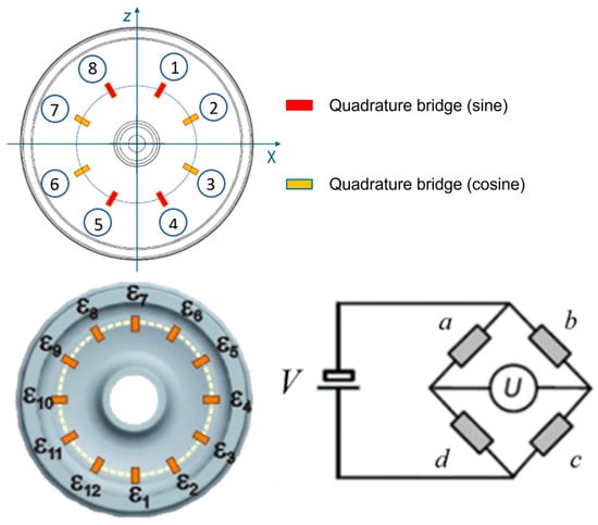
Figure 2.
Examples of strain gauges layout. Wheel-web schematic representation for quadrature (top) and distributed layout (bottom).
Model Description and Simulation Methods
In this section a brief overview of the main components of a railway vehicle is presented to introduce the simplified model hereafter adopted. A conventional passenger coach features a two-level suspension system. The vertical configuration consists of four unsuspended wheelsets, two at the front and two at the rear; two bogies, each housing a pair of wheelsets, providing steering capability and an intermediate level of suspension; finally, the carbody, which is the main suspended mass. The suspension system is structured in two levels. The first level is the primary suspension, and it is located between wheelsets and bogies. It is composed of four vertical springs and four dampers. The second level is the secondary suspension, located between bogies and carbody. It consists of two vertical springs and two dampers per bogie. For high-speed vehicles the architecture may differ slightly [24]. Excluding the simplest dot-mass (1-DOF) model [8], multi degrees of freedom (MDOF) models are often necessary to accurately capture the dynamic behaviour of a railway coach. In this research, a 3-DOF half-coach model is adopted [45]. A detailed schematic representation is available in Figure 3. It consists of an equivalent unsuspended mass, representing the combined mass of two wheelsets acting on a single bogie, a suspended bogie mass, and a suspended half-carbody mass. These masses are interconnected by equivalent springs and dampers, representing the primary and secondary suspension systems. The model is specifically designed for the simulation of vertical vehicle dynamics and the estimation of equivalent wheel vertical displacement using contact forces as input instead of accelerations, which are instead commonly used in similar applications. Thus, only vertical motion is considered. On the contrary, out-of-plane displacements and rotational inertia effects are neglected. As a result, pitch, roll, and yaw motions are not included. Unlike the classic bicycle model commonly used for symmetric road vehicles [46], this model considers half of the railway coach, divided by a vertical and transversal plane passing through the carbody’s centre of gravity. The model’s structure is designed to exploit the existing strain gauges layout which could not be modified. The model takes as input vertical forces recorded by the dedicated TRV used in the Italian Railway track condition monitoring. The outputs are the vertical displacements ui (with i = 1, 2 and 3) of the three masses. Since the primary goal is to estimate the mean vertical displacement of the left and right rail (longitudinal level), only the equivalent wheel movement is analyzed. In the model mweq, mb and mc denote the equivalent wheel, bogie, and half-carbody mass, respectively; k1eq and k2eq represent the equivalent stiffness of primary and secondary suspensions, calculated as a parallel of 4 and 2 springs, respectively; c1eq and c2eq represent the equivalent damping of primary and secondary suspensions, obtained as a parallel of 4 and 2 dampers, respectively; Qi are the four vertical wheel–rail contact forces acting on each wheel of the same bogie. The proposed 3-DOF model can reproduce the vertical dynamics of the three masses within a certain confidence range, as demonstrated in the following sections. This is achieved by focusing on track segments with a constant forward speed and in the context of track geometry monitoring within the D1 wavelength range, which is required by the standards [9].
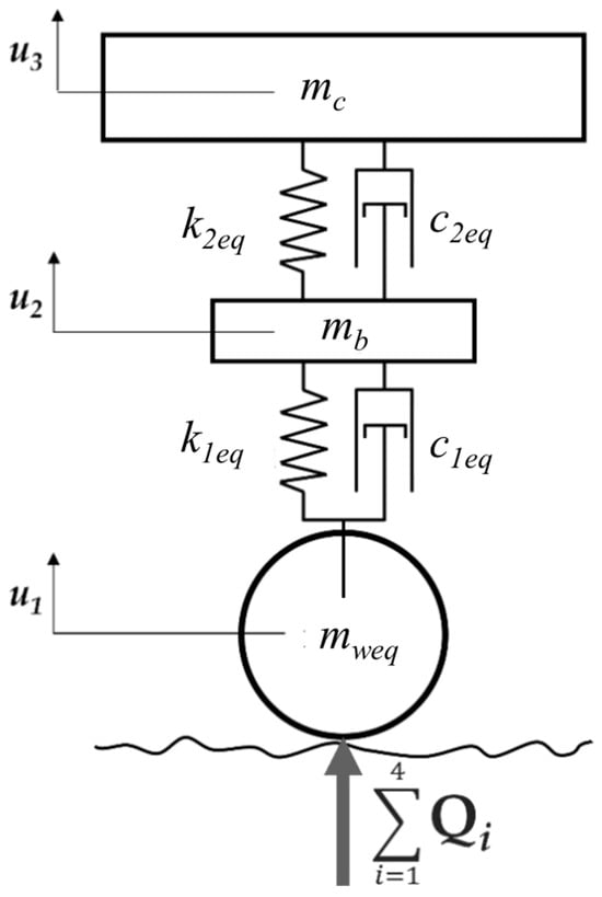
Figure 3.
Schematic representation of the system. Simplified 3-DOF 1/2 a vehicle model, for vertical displacement estimation only.
Setting up a high-DOF model requires considerable effort, making it impractical for certain applications, especially for embedded and real time. Moreover, when the objective is to estimate vertical rail displacements filtered according to a wavelength range, the advantages of a high-DOF model become less relevant, considering the drawback of the high computational cost. In such cases, the performance of simpler models outweighs the need for absolute precision, particularly due to their significantly faster computation time. The comparison between the 3-DOF model and actual TRV measurements highlights the impact of data filtering on accuracy. Filtering the data according to standardized wavelength ranges (such as D1) effectively reduces the bias between measured and simulated displacements. As shown in the results and discussion section, pre-filtering the data makes TRV measurements closely resemble the simulated results, whereas raw data exhibit a more noticeable discrepancy with simulated values. This demonstrates that achieving accuracy comparable to a multi-body model is unnecessary in this context. The proposed model inherently introduces geometric filtering effects [47], like those identified by Yeo et al. [48] and shown in Figure 4. These effects must be considered when evaluating the model’s overall performance in representing measured vertical displacements of the track. Geometric filtering such as the bogie spacing and wheelbase, affects the model’s output. Specifically, for wavelengths close to the wheelbase and double wheelbase length (approximately 3 and 6–7 m, respectively), discrepancies may arise between the model’s signals and those measured by the TRV. This occurs because the wheelbase naturally acts as a geometric low-pass filter in the spatial domain, attenuating vertical variations for track features smaller than 3 m. Examples of these implications are illustrated in Figure 4. Moreover, because the sum of the four forces is adopted, the total applied load acting on the equivalent wheel averages the actions on each wheel. Furthermore, rotations are neglected by hypothesis, potentially leading to other mismatching between simulation and measurements.
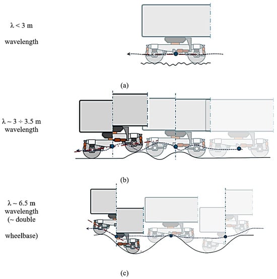
Figure 4.
Example of geometric filtering of the vertical alignment [48], λ refers to wavelength.
With these assumptions, such a simplified 3-DOF model of half-a-coach is used to simulate the dynamic behaviour of the vehicle’s suspension system: the corresponding implementation is shown in the scheme of Figure 5. All the simplifications are reasonable considering portion of track with approximately constant speed, which is true for most of the cruising sections of many ordinary and high-speed lines. To address low-frequency noise, a second order linear Butterworth high-pass filter with 0.1 Hz cut off frequency is applied to the recorded input forces to prevent output signal drift caused by slow-varying or non-zero mean terms during the integration process, while a second order linear Butterworth bandpass filter, with a passband from 3 m to 25 m, corresponding to the D1 range, is applied in the space domain to the estimated equivalent wheel, and measured track vertical displacement for comparison, as prescribed by the standards [9].
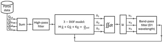
Figure 5.
Schematic representation of the process.
Filtering also improves the robustness of proposed estimator with respect of measurement errors of the instrumented wheelset:
- Unavoidable offsets in force measurements are removed by the high-pass filter (see Figure 5).
- Gain errors on measured forces are small. Their near influence is almost negligible.
- High-frequency errors introduced by noise and bandwidth limits of the measurement system are rejected by the bandpass filter (see Figure 5) and by the intrinsic nature of the 3-DOF model implemented by the estimator (a double stage integration associated with additional poles at few Hertz).
In Figure 5 are front right and left, and rear right and left vertical contact forces; M, C, and K are mass, damping, and stiffness matrix, respectively; ,, and are the 3 masses’ vertical accelerations, speeds, and displacements. By neglecting the rotational inertia of the bodies and considering only vertical displacements, the equations of motion for the three masses are solved according to the scheme in Figure 5, and the wheel displacement is obtained by double-integrating the accelerations over time. More details on the numerical integration are given in Appendix A. The resulting displacements are then compared to the mean vertical rail displacement obtained by averaging the longitudinal level between the left and right rails of a line survey. Line longitudinal level is included in the datasets. As shown in Figure 1, the TRV is equipped with optical measurement systems that acquire real-time track geometry data, which serve as reference for validating the proposed method.
Parameters resulting from the optimization are summarized in Table 2.
Table 2.
Optimized model parameters for the vehicle speed of 160 km/h and D1 range.
A track section of nearly 30 km (dataset 1 in Table 3), consisting of both curved and straight track, and average constant train speed of 160 km/h has been used for the optimization of the model’s parameters, obtaining the best fitting values for suspensions and masses, meaning stiffnesses, damping, and masses for the coach model.
Table 3.
Nomenclature and characteristics of parsed datasets.
Optimization is performed using the Matlab-Simulink Response Optimizer™ (version 2025A), a tool that essentially applies a robust gradient-based search to minimize the least-squares error between a reference signal (experimental data in our case) and a target signal (numerical model results). It is noteworthy that, at the beginning of the calibration process, the actual characteristics of the measurement train were deliberately withheld by the industrial partner that provided the experimental force measurements. Consequently, the performance achieved by the proposed estimator was obtained through self-calibration on the experimental dataset. This represents an important result for the application of the proposed methodology in operational scenarios where vehicle parameters are unknown or significantly perturbed with respect to their nominal values.
Other three mixed track sections of 100, 160, and 200 km/h constant train speed have been used for validating the model and the parameters in a wider range of speeds.
Corresponding datasets are described in Table 3. Available calibration and validation datasets correspond to extended runs in which the recorded speed of the train is substantially constant with coasting or moderate longitudinal forces are applied. Datasets are referred to different lines with modest curvatures and slopes that are statistically common on the Italian network. Once calibrated, model parameters, as reported, were subsequently utilized for all the validation process.
The authors acknowledge that a substantial body of research exists on the use of acceleration measurements as input for estimating rail-track geometry through double integration of the equations of motion. However, to the best of our knowledge, no previous study has employed measured contact forces as the primary input for this purpose. Therefore, IWS, although a well-established technology for homologation and testing, represents a novel approach to track condition monitoring. The present work aims to explore the feasibility of using IWS as an alternative or complementary tool to existing diagnostic technologies—such as accelerometers, rate gyros, and laser scanners—by assessing their capabilities for condition-monitoring tasks. A key aspect of this study is the adoption of a reduced order vehicle model, starting from a 1-DOF configuration and progressively extending it to the current 3-DOF setup, to seek an effective trade-off between simplicity, reliability, and accuracy. As highlighted in the literature, most related works rely on multibody simulations for vehicle–track interaction modelling, and only few employ reduced DOF models, rarely with fewer than five degrees of freedom. Although a comprehensive experimental comparison between IWS-based and accelerometer-based approaches is still required—an activity outside the scope of the present study—this work provides a first assessment of the potential of IWS for this application. Certain features of IWS deserve attention: unlike accelerometer-based approaches, IWS measurements are not affected by the double filtering effect of primary and secondary suspensions, which is inherent in bogie- and carbody-mounted acceleration data. On the other hand, axle-box (and, more generally, bogie and carbody) acceleration signals are known to exhibit low signal-to-noise ratios in service conditions [49,50], which necessitate advanced filtering and identification strategies—such as Vold–Kalman filtering (VKF), band-pass (BP), or high-pass (HPF) filtering—before meaningful interpretation. Therefore, it would be premature to assume that ABA measurements are inherently more accurate than IWS data without a direct, controlled comparison.
5. Results and Discussion
As illustrated in Figure 6, showcasing a visual comparison of an extract of recorded and simulated time series, the model closely mimics data measured by the TRV. By solving the linear system which mathematically represents the model, vertical wheel’s displacements have been obtained and filtered, as previously discussed, using Matlab 2025A. For data confidentiality, all results and measurements of Figure 6 have been normalized with the maximum value of the measured mean vertical alignment, which is dependent on the specific dataset. Although a clear underestimation of the output’s magnitude is obtained for negative displacements, and a light overestimation of positive peaks can be identified, both waveform and wavelength of the simulated displacements are closely related to the reference data. The highest errors are observed at lower speeds (dataset 4). The primary reason for this behaviour is likely related to the filtering of static force contributions, which are unavoidable when estimating vertical displacements from contact force or acceleration measurements. This is reasonable because the proposed procedure involves the double integration of real-world recorded signals, which are affected by small offsets and low-frequency dynamics associated with unmodelled degrees of freedom (DOFs) of the actual vehicle. In the proposed methodology, these contributions are currently filtered out using high-pass and band-pass filters operating purely in the time domain. These filters will be replaced by more sophisticated disturbance estimators, which are the subject of ongoing and future research activities. Furthermore, low-frequency load transfers could be better captured by increasing the number of modelled DOFs, thus achieving an improved trade-off between model complexity and estimation accuracy. The solution proposed in the present work achieves good accuracy despite the extreme simplification of the vehicle dynamics and the limited number of parameters and data required for its implementation or calibration. Also, some discrepancies between predicted displacements and measured ones are recorded in a narrow band of frequencies of about 8 Hz which is almost invariant with speed. This error is not associated with any modal behaviour of the lumped model or to effects introduced by adopted filters. This is a feature of measured contact forces that are used as input for the proposed model; authors are currently investigating the reason for the presence of this feature.
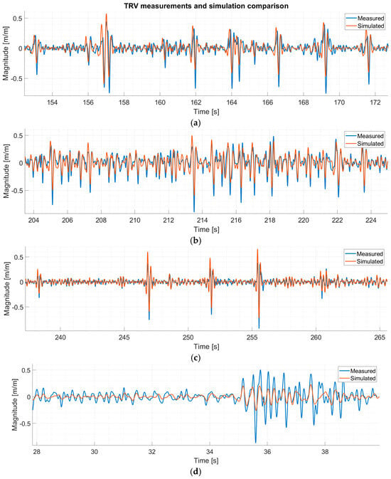
Figure 6.
D1 wavelength range band-pass filtered data. Comparison between reference measured and simulated vertical displacements. Blue line-measured data; red line—simulation; (a) dataset 1; (b) dataset 2; (c) dataset 3; (d) dataset 4.
As shown in Figure 7, a fast Fourier transform (FFT) of the track irregularities measured by the TRV and simulated vertical displacements has been calculated for a comparison of data spectra. The FFT confirms the close relation between experimental and simulated data. In the validity field of the D1 range, for a train speed of 160 km/h (44.4 m/s), the inferior limit corresponds to 1.78 Hz, while the superior limit corresponds to 14.81 Hz for dataset 1.
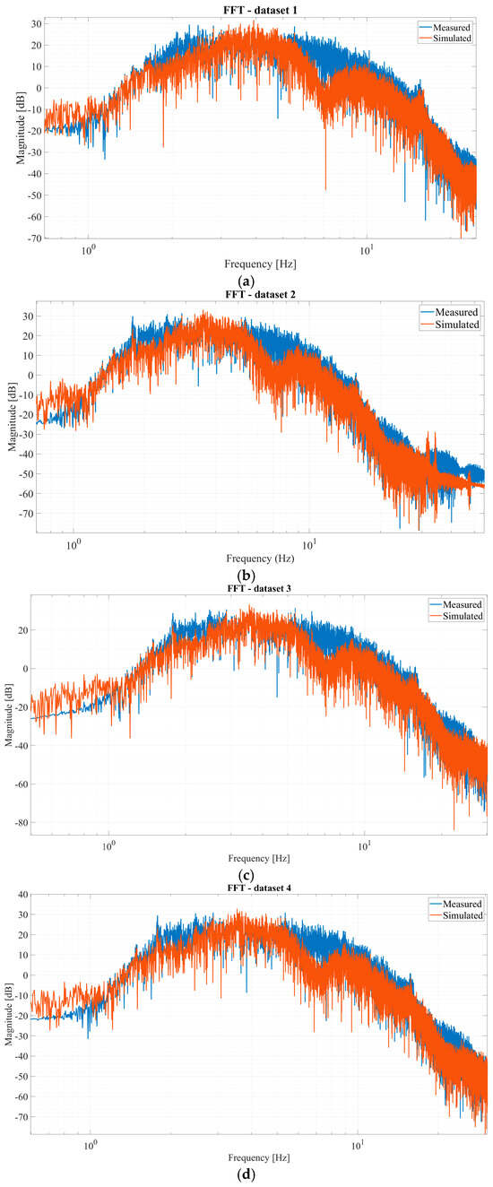
Figure 7.
Spectra comparison of (a) dataset 1; (b) dataset 2; (c) dataset 3; (d) dataset.
6. Error Analysis
An error and correlation analysis has been conducted to evaluate the performance of the model. As the first metrics, absolute residuals (1) and root mean squared error (RMSE) (2) have been calculated between the measured and simulated time series:
Subscript i implies element-wise operation between the two arrays. The results for each parsed track section are summarized in Table 4.
Table 4.
Error and correlation analysis for the recorded and simulated mean vertical alignment.
Residuals and RMSE metrics highlight differences in signal magnitude, but they do not capture the similarity between the simulated and measured average longitudinal level. To address this, a correlation analysis was performed to further validate the model. Pearson correlation coefficient (R) and coefficient of determination (R2) were calculated according to (3) [51]:
with X and Y measured and simulated arrays of n elements, and their mean values, respectively. Model’s performance has been evaluated at two other available train speeds in an attempt of extending the validity range of the proposed model, parsing available datasets 2, 3, and 4, which complies with most of the conventional European railways (fast regional, intercity, cross country, and some high-speed connections); this is depicted on the map available on openrailwaymap.org [52] that is shown in Figure 8.
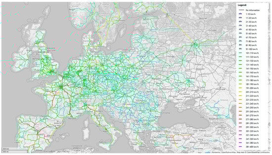
Figure 8.
Map of the railway infrastructure in Europe, grouped by maximum line speed. Green shades represent 90–200 km/h lines.
The high R-value for datasets 1, 2, and 3, confirms the strong correlation between the time series, consistent with the visual comparison and Fourier analysis. Although relatively high, the R2 values suggest areas where the model’s output still deviates from the measured data, particularly in amplitude and frequency, rather than wavelength. These discrepancies, combined with the time delay introduced by the filters, likely contribute to the lower R and R2 scores for datasets 4, despite the overall similarity between the simulated and measured signals. The high RMSE values could be related to the underestimation of the vertical displacement by the model and localized mismatching in the waveform of the signals. Results of datasets 1, 2, and 3 are promising, exhibiting good repeatability. As the travelling speed of the train decreases (dataset 4), the fitting capability of the model also decreases, but it is expected to slowly fall after the 200 km/h limit of dataset 3 too. No useful data over 200 km/h are available to authors. However, the general expected trend in terms of performances seems to be confirmed by further analysis performed on some not significant datasets (durations of about 30–90 s) for which R is also calculated, as shown in Figure 9. These additional data (red dots) have not been used to generate the interpolating curve, but their distribution at least supports the idea that the chosen interpolating curve is good enough.
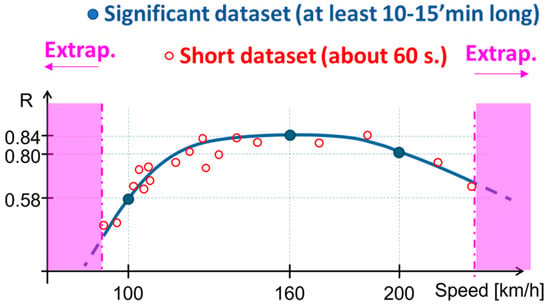
Figure 9.
Expected behaviour of the R value for the investigated train speed range, showcasing the applicability range of the model.
7. Conclusions and Future Developments
In this paper a simplified 3-DOF linear model of half-a-coach train for estimating the vertical displacement of the wheels, and consequently the longitudinal level of the track in the D1 range (3–25 m wavelength) using force recordings, is proposed. Despite its simplicity, the method has proven to provide significant results for the estimation of D1 vertical irregularities in a range of speed comprise between 100 and 200 km/h when tested with real experimental data. The performed analysis is focused solely on vertical motion. High-pass filters have been applied to remove low-frequency inaccuracies in the force recordings, which arise from uncertainties in the measurements. This approach effectively filtered out non-zero mean terms and retained only the high-frequency content of the excitation signals. The equations of motion for the 3-DOF system were solved by double integrating the accelerations, and the resulting mean displacements were compared with a reference mean vertical alignment calculated from the measurements of TRV used for track geometry monitoring and diagnosis. A visual comparison of the time series and spectra showed a high degree of correlation between the two datasets. The error analysis indicated the presence of inaccuracies by the means of residual values, attributable to amplitude and phase mismatches between the measured and simulated displacements. The error analysis revealed inaccuracies in terms of the maximum residual value, mainly attributable to amplitude and phase mismatches between the measured and simulated displacements. These discrepancies arise from the reduced number of modelled DOFs which, while being the main source of error, also represents the strength of the proposed approach, as it requires negligible computational resources and only limited technical information regarding track, wheel–rail contact, and suspensive system. For this reason, the proposed functionality can be considered a low-cost add-on that can be easily integrated into measurement setups where wheel–rail contact force measurements are performed, to further refine the outputs of optical devices.
The neglected inertias and rotational effects, particularly pitch motion, are believed to be the primary cause of the reduced performance of the proposed estimator, especially in scenarios where dynamic load transfers between wheelsets are expected to increase (e.g., narrow curves, high longitudinal accelerations, and decelerations). Additionally, the applied filters, as shown in Figure 5, introduce a further degree of approximation. These filters are currently implemented in the time (or space) domain, with their poles continuously adjusted according to train speed in order to capture the desired wavelengths of the railway track irregularities. While this approach is suitable for smooth and slowly varying vehicle speeds, it leads to an increase in estimation errors when significant longitudinal accelerations or decelerations occur.
The discrepancies in waveform and amplitude between the simulated and recorded data, along with the time delay introduced by the filters, may also account for lowering the R and R2 coefficients obtained for dataset 3 and dataset 4, used for the validation of the model. However, results are promising, showing good agreement with experimental data, making the proposed method suited for the analysis of data recorded between 100 and 200 km/h. The high R coefficient for datasets 1 and 2, and the still relatively high value obtained for dataset 3 and 4, highlights the good performance and the potential of the simplified model in a wide range of train speed, accounting for many of the ordinary railway lines and some high-speed interconnections. Minor adjustments and improvements to the model could lead to the development of a rapid and straightforward tool for the estimation of the mean vertical alignment based solely on force recordings. Given the non-stationary speed of the train, future work will focus on correcting the delay and distortion introduced in the simulation results by the filters, aiming to improve the correlation between simulated and reference signals. By extending the model to 6-DOF (5 + 1 constrained), accounting for 2 bogies with 2 equivalent wheels and an entire coach, considering its rotational inertia and pitch motion, a more precise model can be implemented with the introduction of a Kalman filter [53] that should be useful for multiple purposes:
- Calibrate model parameters when uncertain or partially known
- Self-calibration and optimal filtering with respect of speed, line conditions on other external disturbances
- Data fusion with additional measurements from inertial or optical sensors further improving measurement precision and reliability.
Additionally, the study could be extended to investigate the lateral motion of the wheelsets for rail alignment estimation, following a similar methodology as discussed herein. These efforts will contribute to the broader adoption of IWS for condition monitoring and diagnostics. When combined with optical devices, this approach may yield significant benefits for the railway maintenance sector and track geometry condition monitoring, utilizing both TRVs and in-service vehicles. The potential to use force recordings for reconstructing the mean vertical alignment of the track is evident, and the adopted method is consistent with reference data, as supported by error and correlation analysis. However, it is important to note that existing standards impose limits on the maximum permissible values for geometric parameters. Therefore, the mean value derived using the proposed method may lead to an underestimation of the actual track condition. This aspect will be carefully considered in the development of a vertical motion estimation algorithm based on the proposed simplified model.
Author Contributions
G.B., conceptualization, methodology, software, validation, formal analysis, investigation, data curation, writing—original draft, visualization; M.E., conceptualization, methodology, writing—review and editing; P.F.W., conceptualization, methodology, writing—review and editing; L.P., project administration, funding acquisition, resources, supervision, methodology, writing—review and editing. All authors have read and agreed to the published version of the manuscript.
Funding
This research received no external funding.
Data Availability Statement
Data and Models are available only after contacting the coordinator of the project Luca Pugi distinguishing between parts that can be fully disclosed and parts for which some mutual agreement is needed.
Acknowledgments
The authors wish to thank the industrial partner who provided anonymous data from a real measurement setup. Without their support, this work would not have been possible. All individuals included in this section have consented to the acknowledgement.
Conflicts of Interest
The authors declare no conflicts of interest.
Abbreviations
The following abbreviations are used in this manuscript:
| TRV | Track Recording Vehicle |
| DOF | Degree of Freedom |
| MDOF | Multi Degree of Freedom |
| TG | Track Geometry |
| FFT | Fast Fourier Transform |
| FE | Finite Element |
| IWS | Instrumented Wheelsets |
| BP | Band-Pass |
| HPF | High-Pass Filter |
| VKF | Vold–Kalman Filtering |
Appendix A
Linear State Space Representation of the Half-a-Coach Vehicle Model
The model has been optimized on MATLAB Simulink’s Parameter Optimization App, by minimizing the trade-off between the model state space output and the reference data. Appendix A shows the equivalent state space representation used to solve the linear model of half-a-coach vehicle, check the results, and obtain the plots.
In the state space representation x is the state vector and its first derivative; y is the output vector; q is the input vector, of which Q is the load vector containing vertical forces Qi; subscripts f and r denote front and rear, respectively, while subscripts R and L denote right and left side, respectively; A is the system matrix, B is the input matrix, C is the output matrix, and D is the feedthrough matrix. For this representation, given the linearity of the system, the second order linear Butterworth high-pass filter with cut-off frequency of 0.1 Hz is applied to the output signal instead of the input contact forces used for the simulation. Obtained vertical displacements are then filtered in the D1 wavelength range with a second order linear Butterworth band-pass filter, with cut of wavelengths of 25 and 3 m, respectively (1.78 and 14.81 Hz) for the vehicle speed of 160 km/h (44.44 m/s).

Figure A1.
Schematic representation of the state space model.
Figure A1.
Schematic representation of the state space model.

References
- European Commission. EU Transport in Figures: Statistical Pocketbook 2024; Mobility and Transport, Publications Office of the European Union: Luxembourg, 2024; ISBN 978-92-68-19812-4. [Google Scholar] [CrossRef]
- Ward, C.P.; Weston, P.F.; Stewart, E.J.C.; Li, H.; Goodman, C.J.; Roberts, C. Condition Monitoring Opportunities Using Vehicle-Based Sensors. Proc. Inst. Mech. Eng. Part F J. Rail Rapid Transit 2011, 225, 202–218. [Google Scholar] [CrossRef]
- CIFI. La Diagnostica Mobile e le Misure per la Certificazione. Webinar, 31 January 2022. Available online: https://www.cifi.it/UplDocumenti/Roma31012022/Presentazione%20Bonafe_Palmiotto%20CIFI%202022-01-31.pdf (accessed on 7 January 2025).
- MERMEC Group. I Rotabili di RFI—Il Treno Archimede. Available online: https://www.mermecgroup.com/press-room/media-coverage/420/i-rotabili-di-rfi-il-treno-archimede.php (accessed on 7 January 2025).
- Gomez, E.; Giménez, J.G.; Alonso, A. Method for the Reduction of Measurement Errors Associated to the Wheel Rotation in Railway Dynamometric Wheelsets. Mech. Syst. Signal Process. 2011, 25, 3062–3077. [Google Scholar] [CrossRef]
- Nielsen, J.C.O. High-Frequency Vertical Wheel–Rail Contact Forces—Validation of a Prediction Model by Field Testing. Wear 2008, 265, 1465–1471. [Google Scholar] [CrossRef]
- Ronasi, H.; Johansson, H.; Larsson, F. Identification of Wheel–Rail Contact Forces Based on Strain Measurements, an Inverse Scheme and a Finite-Element Model of the Wheel. Proc. Inst. Mech. Eng. Part F J. Rail Rapid Transit 2014, 228, 343–354. [Google Scholar] [CrossRef]
- Bellacci, G.; Entezami, M.; Weston, P.; Baldanzini, N.; Pugi, L. Evaluating the Feasibility of Estimating Rail Longitudinal Level Through Double Integration of Vertical Contact Forces. Mech. Mach. Sci. 2025, 180, 607–614. [Google Scholar] [CrossRef]
- EN 13848-1:2019; Railway Applications—Track—Track Geometry Quality—Part 1: Characterization of Track Geometry. European Committee for Standardization (CEN): Brussels, Belgium, 2019.
- EN 14363:2022; Railway Applications—Testing and Simulation for the Acceptance of Running Characteristics of Railway Vehicles—Running Behaviour and Stationary Tests. European Committee for Standardization (CEN): Brussels, Belgium, 2022.
- Thong, Y.K.; Woolfson, M.S.; Crowe, J.A.; Hayes-Gill, B.R. Numerical Double Integration of Acceleration Measurements in Noise. Measurement 2004, 36, 73–92. [Google Scholar] [CrossRef]
- Lewis, R.B.; Richards, A.N. A Compensated Accelerometer for the Measurement of Railway Track Crosslevel. IEEE Trans. Veh. Technol. 1988, 37, 174–178. [Google Scholar] [CrossRef]
- Weston, P.F.; Ling, C.S.; Goodman, C.J.; Roberts, C.; Li, H.; Goodall, R.M. Monitoring Vertical Track Irregularity from In-Service Railway Vehicles. Proc. Inst. Mech. Eng. Part F J. Rail Rapid Transit 2007, 221, 75–88. [Google Scholar] [CrossRef]
- Weston, P.F.; Ling, C.S.; Goodman, C.J.; Roberts, C.; Li, H.; Goodall, R.M. Monitoring Lateral Track Irregularity from In-Service Railway Vehicles. Proc. Inst. Mech. Eng. Part F J. Rail Rapid Transit 2007, 221, 89–100. [Google Scholar] [CrossRef]
- Zschiesche, K.; Reiterer, A. Optical Measurement System for Monitoring Railway Infrastructure—A Review. Appl. Sci. 2024, 14, 8801. [Google Scholar] [CrossRef]
- Soilán, M.; Sánchez-Rodríguez, A.; del Río-Barral, P.; Pérez-Collazo, C.; Lorenzo, H.; Arias, P. Review of Laser Scanning Technologies and Their Applications for Road and Railway Infrastructure Monitoring. Infrastructures 2019, 4, 58. [Google Scholar] [CrossRef]
- CIFI. CIFI Documents and Webinars. Available online: https://www.cifi.it/UplDocumenti/WebinarCIFI23112020-Dalla%20manutenzione%20ciclica%20alla%20predittiva.pdf (accessed on 7 January 2025).
- Rosano, G.; Massini, D.; Bocciolini, L.; Zappacosta, C.; Di Gialleonardo, E.; Somaschini, C.; La Paglia, I.; Pugi, L. Diagnostics of the Railway Track—Possibility of Development through the Measurement of Accelerations and Contact Forces. Ing. Ferrov. 2024, 79, 81–102. [Google Scholar] [CrossRef]
- Bellacci, G.; Pugi, L.; Baldanzini, N. Validation of a Wheelset Finite Element Model for Static Structural Analysis and Inverse Force Identification. In Latest Advancements in Mechanical Engineering; ISIEA 2024. Lecture Notes in Networks and Systems; Concli, F., Maccioni, L., Vidoni, R., Matt, D.T., Eds.; Springer: Cham, Switzerland, 2024; Volume 1124, pp. 236–244. [Google Scholar] [CrossRef]
- Ronasi, H.; Nielsen, J.C.O. Inverse Identification of Wheel–Rail Contact Forces Based on Observation of Wheel Disc Strains: An Evaluation of Three Numerical Algorithms. Veh. Syst. Dyn. 2012, 51, 74–90. [Google Scholar] [CrossRef]
- Bracciali, A.; Cavaliere, F.; Macherelli, M. Review of Instrumented Wheelset Technology and Applications. In Proceedings of the Second International Conference on Railway Technology: Research, Development and Maintenance; Pombo, J., Ed.; Civil-Comp Press: Stirlingshire, UK, 2014. [Google Scholar]
- Bellacci, G.; Neri, F.; Pugi, L.; Giachetti, A.; Barlacchi, E.; Baldanzini, N. Preliminary Frequency Response Analysis of a Contact Force Measurement System for Rail Applications. In Applications in Electronics Pervading Industry, Environment and Society; ApplePies 2023; Bellotti, F., Grammatikakis, M.D., Mansour, A., Roch, M.R., Seepold, R., Solanas, A., Berta, R., Eds.; Lecture Notes in Electrical Engineering, Volume 1110; Springer: Cham, Switzerland, 2024; pp. 240–247. [Google Scholar] [CrossRef]
- Italcertifer. Estensimetria, Sale e Pantografi Strumentati. Available online: https://www.italcertifer.com/it/laboratori/estensimetria--sale-e-pantografi-strumentati-.html (accessed on 7 January 2025).
- Iwnicki, S.; Spiryagin, M.; Cole, C.; McSweeney, T. Handbook of Railway Vehicle Dynamics, 2nd ed.; CRC Press: Boca Raton, FL, USA, 2019. [Google Scholar] [CrossRef]
- Abeidi, A.S.; Bosso, N.; Gugliotta, A.; Somà, A. Numerical Simulation of Wear in Railway Wheel Profiles. In Proceedings of the ASME 8th Biennial Conference on Engineering Systems Design and Analysis (ESDA 2006), Torino, Italy, 4–7 July 2006; Volume 3: Dynamic Systems and Controls, Symposium on Design and Analysis of Advanced Structures, and Tribology. ASME: Torino, Italy, 2006; pp. 963–977. [Google Scholar] [CrossRef]
- Bosso, N.; Magelli, M.; Zampieri, N. Simulation of Wheel and Rail Profile Wear: A Review of Numerical Models. Railw. Eng. Sci. 2022, 30, 403–436. [Google Scholar] [CrossRef]
- Logozzo, S.; Valigi, M.C. Green Tribology: Wear Evaluation Methods for Sustainability Purposes. Int. J. Mech. Control. 2022, 23, 23–34. [Google Scholar]
- Logozzo, S.; Valigi, M.C. Wear Assessment and Reduction for Sustainability: Some Applications. In Mechanisms and Machine Science; Springer: Cham, Switzerland, 2022; Volume 108, pp. 395–402. [Google Scholar] [CrossRef]
- EN 13848-2:2020; Railway Applications—Track—Track Geometry Quality—Part 2: Measuring Systems—Track Recording Vehicles. European Committee for Standardization (CEN): Brussels, Belgium, 2020.
- Hernández, W. Improving the Responses of Several Accelerometers Used in a Car Under Performance Tests by Using Kalman Filtering. Sensors 2001, 1, 38–52. [Google Scholar] [CrossRef]
- Sun, Y.Q.; Dhanasekar, M. A Dynamic Model for the Vertical Interaction of the Rail Track and Wagon System. Int. J. Solids Struct. 2002, 39, 1337–1359. [Google Scholar] [CrossRef]
- Zhai, W.; Cai, Z. Dynamic Interaction between a Lumped Mass Vehicle and a Discretely Supported Continuous Rail Track. Comput. Struct. 1997, 63, 987–997. [Google Scholar] [CrossRef]
- Kawasaki, J.; Youcef-Toumi, K. Estimation of Rail Irregularities. In Proceedings of the 2002 American Control Conference, Anchorage, AK, USA, 8–10 May 2002. [Google Scholar]
- Mori, H.; Tsunashima, H.; Kojima, T.; Matsumoto, A.; Mizuma, T. Condition Monitoring of Railway Track Using In-Service Vehicle. J. Mech. Syst. Transp. Logist. 2012, 3, 154–165. [Google Scholar] [CrossRef]
- Odashima, M.; Azami, S.; Naganuma, Y.; Mori, H. Track Geometry Estimation of a Conventional Railway from Car-Body Acceleration Measurement. Mech. Eng. J. 2017, 4, 16–00498. [Google Scholar] [CrossRef]
- Alfi, S.; Bruni, S. Estimation of Long Wavelength Track Irregularity from Onboard Measurement. In Proceedings of the 4th IET International Conference on Railway Condition Monitoring (RCM 2008), London, UK, 18–20 June 2008; pp. 1–6. [Google Scholar] [CrossRef]
- Miwa, M.; Kawasaki, Y.; Yoshimura, A. Influence of Vehicle Unsprung-Mass on Dynamic Wheel Load. In Computers in Railways XI—Computer System Design and Operation in the Railway and Other Transit Systems; Allan, J., Arias, E., Brebbia, C.A., Goodman, C., Rumsey, A.F., Sciutto, G., Tomii, N., Eds.; WIT Press: Southampton, UK, 2008; Volume 103, pp. 715–724. [Google Scholar]
- Tsunashima, H. Condition Monitoring of Railway Tracks from Car-Body Vibration Using a Machine Learning Technique. Appl. Sci. 2019, 9, 2734. [Google Scholar] [CrossRef]
- La Paglia, I.; Di Gialleonardo, E.; Facchinetti, A.; Carnevale, M.; Corradi, R. Acceleration-based condition monitoring of track longitudinal level using multiple regression models. Proc. Inst. Mech. Eng. Part F J. Rail Rapid Transit 2024, 238, 479–488. [Google Scholar] [CrossRef]
- De Rosa, A.; Kulkarni, R.; Qazizadeh, A.; Berg, M.; Di Gialleonardo, E.; Facchinetti, A.; Bruni, S. Monitoring of Lateral and Cross Level Track Geometry Irregularities through Onboard Vehicle Dynamics Measurements Using Machine Learning Classification Algorithms. Proc. Inst. Mech. Eng. Part F J. Rail Rapid Transit 2021, 235, 107–120. [Google Scholar] [CrossRef]
- Ghiasi, R.; Khan, A.M.; Sorrentino, D.; Diaine, C.; Malekjafarian, A. An Unsupervised Anomaly Detection Framework for Onboard Monitoring of Railway Track Geometrical Defects Using One-Class Support Vector Machine. Eng. Appl. Artif. Intell. 2024, 133, 108167. [Google Scholar] [CrossRef]
- Gullers, P.; Dreik, P.; Nielsen, J.C.O.; Ekberg, A.; Andersson, L. Track Condition Analyser: Identification of Rail Rolling Surface Defects Likely to Generate Fatigue Damage in Wheels Using Instrumented Wheelset Measurements. Proc. Inst. Mech. Eng. Part F J. Rail Rapid Transit 2011, 225, 1–13. [Google Scholar] [CrossRef]
- Diana, G.; Resta, F.; Braghin, F.; Bocciolone, M.; Di Gialleonardo, E.; Crosio, P. Methodology for the Calibration of Dynamometric Wheelsets for the Measurement of the Wheel–Rail Contact Forces. Ing. Ferrov. 2012, 67, 9–21. [Google Scholar]
- Velletrani, F.; Licciardello, R.; Bruner, M. Intelligent Wheelsets for the Trains of the Future: The Role of In-Service Wheel–Rail Force Measurement. Ing. Ferrov. 2020, 75, 701–725. [Google Scholar]
- Evans, J.R. The Modelling of Railway Passenger Vehicles. Veh. Syst. Dyn. 2007, 20, 144–156. [Google Scholar] [CrossRef]
- Wong, J.Y. Theory of Ground Vehicles, 3rd ed.; John Wiley & Sons: New York, NY, USA, 2001. [Google Scholar]
- Dragoș, S.; Madalina, D.; Mihai, L. The Geometric Filtering Effect on Ride Comfort of the Railway Vehicles. UPB Sci. Bull. Ser. D Mech. Eng. 2021, 83, 137–154. [Google Scholar]
- Yeo, G.J.; Weston, P.F.; Roberts, C. The Utility of Continual Monitoring of Track Geometry from an In-Service Vehicle. In Proceedings of the 6th IET Conference on Railway Condition Monitoring (RCM 2014), Birmingham, UK, 17–20 November 2014; pp. 1–6. [Google Scholar]
- Hoelzl, C.; Dertimanis, V.; Ancu, L.; Kollros, A.; Chatzi, E. Vold–Kalman Filter Order Tracking of Axle Box Accelerations for Track Stiffness Assessment. Mech. Syst. Signal Process. 2023, 204, 110817. [Google Scholar] [CrossRef]
- Pieringer, A.; Kropp, W. Model-Based Estimation of Rail Roughness from Axle Box Acceleration. Appl. Acoust. 2022, 193, 108760. [Google Scholar] [CrossRef]
- Howell, D.C. Statistical Methods for Psychology, 7th ed.; Wadsworth, Cengage Learning: Belmont, CA, USA, 2009. [Google Scholar]
- OpenRailwayMap. Available online: https://www.openrailwaymap.org/ (accessed on 7 January 2025).
- Locorotondo, E.; Lutzemberger, G.; Pugi, L. State-of-charge estimation based on model-adaptive Kalman filters. Proc. Inst. Mech. Eng. Part I J. Syst. Control Eng. 2021, 235, 1272–1286. [Google Scholar] [CrossRef]


Disclaimer/Publisher’s Note: The statements, opinions and data contained in all publications are solely those of the individual author(s) and contributor(s) and not of MDPI and/or the editor(s). MDPI and/or the editor(s) disclaim responsibility for any injury to people or property resulting from any ideas, methods, instructions or products referred to in the content. |
© 2025 by the authors. Licensee MDPI, Basel, Switzerland. This article is an open access article distributed under the terms and conditions of the Creative Commons Attribution (CC BY) license (https://creativecommons.org/licenses/by/4.0/).