Prediction and Optimization of Interference Fit Level in Slug Riveted Structure with Deep Learning Enhanced Genetic Algorithm

Abstract

The interference fit connection with slug rivets is widely used in aircraft assembly, and an appropriate interference value is vital for aircraft structural integrity. This study proposed a prediction–optimization framework that a deep neural network (DNN) surrogate was trained on a parametric finite element dataset to regress four interference measurements (G1–G4), and the trained DNN was embedded into a genetic algorithm (GA) to search process parameters that meet prescribed target interference. An orthogonal design with range analysis was employed to rank factor importance and provide interpretable trends, while finite element model (FEM) re-runs were used for validation. Compared with support vector regression, random-forest regression, and Bayesian regression, the DNN demonstrated superior fitting accuracy and a more favorable error distribution on held-out data. GA solutions obtained using the DNN surrogate achieved the target interference with a maximum relative deviation of 9.75%, confirming the effectiveness of the proposed workflow for rapid, physics-consistent interference control. The contributions of the study were as follows: (i) an end-to-end, quick-response, reproducible FEM→DNN→GA pipeline for slug-rivet interference; (ii) quantitative factor ranking with mechanistic interpretation; and (iii) minute-scale parameter optimization suitable for engineering deployment.

1. Introduction

Interference riveting technology is a commonly employed connection method in aerospace manufacturing. The interference fit at the contact interface between the rivet and the hole wall ensures a uniform load distribution, which significantly enhances the fatigue life of riveted structures and improves the sealing reliability at the connection points [1,2]. There are many factors affecting the interference fit level [3], and it is difficult to construct a multivariate nonlinear relationship between the factors and the interference value. Currently, interference values are primarily studied by conducting experiments prior to mass production and by measuring the values corresponding to known process parameter combinations. However, the above method is time-consuming and costly, while heavily relying on the experience of engineers. It is essential to conduct some research on predicting the interference values quickly and accurately, as well as optimizing the riveting parameters.

Generally, based on riveting process analysis, a mechanism model was established to predict the deformation behavior of the rivet and connected plates, thereby controlling the connection quality of the riveted joints. Scholars have conducted extensive research in this field using various methods, such as plastic mechanics, finite element analysis (FEA), and fracture mechanics. Lv et al. [4] proposed a theoretical analysis method for the nonlinear dynamic plastic behavior of riveted structures, applicable to predicting the forming quality of riveted structures under varying extrusion forces, speeds, and materials. Liang et al. [5] investigated the effect of die angle on the fatigue life of riveted joints through a combination of FEA and experimental validation, and found that variations in rivet angles resulted in different residual stress distributions, which significantly affected the fatigue performance. Tian et al. [6] analyzed the fatigue life of riveted joints with different countersunk depths using the finite element method. Derijck et al. [7] established a mapping relationship between the riveting force and the driven head size according to the plastic deformation assumption, and validated it through experiments under various materials. Huang et al. [8] proposed a novel fatigue crack growth model based on structural load to predict the fatigue life and the final crack aspect ratio of riveted joints. These studies demonstrated that riveting quality could be effectively predicted from the initial processing conditions. However, in practice, most of these methods involve complex calculations, making it challenging to rapidly predict the riveting quality under new combinations of process parameters.

Data-driven methods are capable of rapidly providing results when confronted with entirely new combinations of process parameters, significantly reducing computational resources and time costs [9]. Deep learning, as an emerging data-driven method, could build complex input–output relationships. The typical structure was composed of a multilayer perceptron with multiple hidden layers, which gradually transforms initial “low-level” feature representations into “high-level” feature representations through multiple layers of processing. Compared with traditional regression model construction methods, the unique advantage of deep learning lies in its high sensitivity to relevant details [10,11]. Belhouchet et al. [12] demonstrated that an Artificial Neural Network (ANN) exhibited higher accuracy in fitting complex relationships compared to mathematical models based on numerous assumptions, and the ANN could provide more reliable prediction results under various process parameter conditions. In recent years, many scholars have conducted related research, demonstrating that deep learning techniques could leverage large datasets to predict defects in the product manufacturing process. Wang et al. [13] proposed a method to evaluate the hydrostatic guideway straightness errors online based on a long short-term memory network model. Deshpande et al. [14] used deep learning for image segmentation in additive manufacturing to detect defects. Additionally, deep learning also serves as a high-precision, low-computational-cost surrogate model to guide the optimization of product process parameters. Sun et al. [15] proposed a computational framework combining ANNs and a genetic algorithm (GA), where ANNs were trained as surrogate models for FEA to accelerate the GA optimization process. Nejad et al. [16] utilized ANNs to fit the relationship between various process parameters and the fatigue life of riveted joints.

The GA is a well-known metaheuristic algorithm that mimics Darwin’s theory of natural selection to perform selection and iteration within a population to achieve the optimal solution [17]. Using metaheuristic algorithms, such as GAs, to select the optimal combination of process parameters is a commonly used method [18]. The advantage of this approach lies in its minimal reliance on detailed structural information for the optimization problem, enabling rapid identification of optimal process parameter combinations. Shi et al. [19] proposed an intelligent matching system for countersunk hole riveting based on the fruit fly optimization algorithm, which significantly improved the control level of the riveting interference value compared to traditional tolerance zone methods. Choudhary et al. [20] designed a hybrid optimization method combining multiple metaheuristic algorithms to optimize the submerged arc welding process parameters, resulting in more favorable parameter settings. Rajendran et al. [21] introduced various metaheuristic algorithms to optimize the process parameters of wire-cut electrical discharge machining, achieving superior results compared to traditional optimization algorithms. Metaheuristic algorithms are also integrated with other techniques for process parameter design. Ni et al. [22] combined the GA and the ant colony algorithm with a finite element model (FEM) to optimize process parameters such as rivet upsetting direction and assembly sequence, thereby controlling assembly errors during the large-scale riveting process. Combined with a deep learning prediction model, Wu et al. [23] employed a GA to generate a Pareto set as an alternative for selecting machining process parameters. Oliveira et al. [24] examined the integration of metaheuristic algorithms with machine learning techniques for optimizing searches in large datasets. The mentioned hybrid approach, through learning from prior iterations, demonstrating learning from prior iterations enhances both efficiency and effectiveness compared to traditional methods.

Interference fit riveting enhances fatigue performance and sealing, while its multi-factor, nonlinear interactions are challenging to explore using finite element analysis or experiments alone. Prior studies have elucidated mechanisms, they remain limited in generalizability and incur high computational costs for new parameter combinations. The challenge was addressed using a data-driven surrogate: a DNN was trained on parametric FEM data to predict G1–G4, which was then embedded in a GA for target-seeking optimization. Factor importance was further quantified via orthogonal design and range analysis, and the optimized settings were validated by FEM re-runs. The contributions of the study were as follows: (i) a reproducible FEM→DNN→GA pipeline, (ii) accuracy gains over SVR/RFR/Bayesian baselines, (iii) interpretable factor ranking showing the leading role of plate yield strength, and (iv) minute-scale optimization to meet target interference levels.

2. Basic Prediction and Optimization Framework

The basic structure of the process parameter optimization framework proposed in this study is illustrated in Figure 1. The specific steps are as follows: (1) Develop a FEM for the riveting process and validate its effectiveness by comparing with experimental results; (2) Conduct orthogonal experiments on selected process parameters to analyze the impact of each parameter on the rivet interference fit level; (3) Design the topology of the DNN, set hyperparameters, train the predictive model, and make comparisons with other regression models to verify its accuracy; (4) Construct a fitness function using the predictive model and the targeted interference fit level, and apply a GA to optimize the process parameters. The quality of the optimized parameter is evaluated through experiments.

2.1. Modeling Process

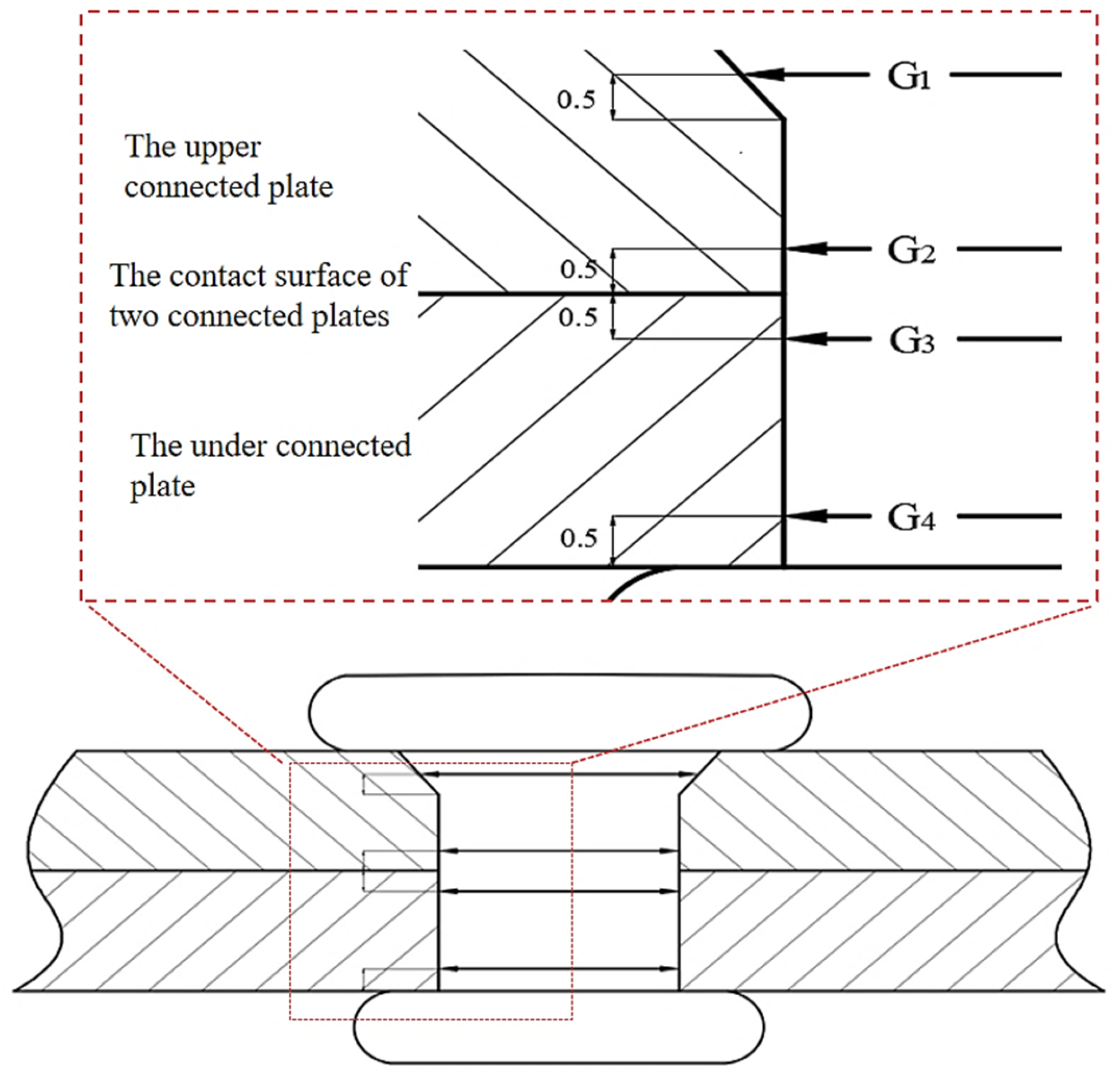
A FEM for the riveting process was established, and its validity was verified through experimental testing. Potential factors included hole diameter tolerance, surface finish, friction, temperature, force profile, plate stack-up, material property parameters, and geometric protrusion. Eight factors dominating interference in automated cells, which are controllable or characterizable in FEM, were selected for analysis. The design space comprised riveting force (F_S), dwell time (t), protrusion (h), clamping force (F_C), as well as material parameters of the connected plates: elastic modulus (E), initial yield stress (A), hardening exponent (n), and hardening constant (B). The locations for interference measurement are shown in Figure 2, and the interference level is represented by four measurement values, G1, G2, G3, and G4, respectively. Corresponding experiments were conducted with the same parameters used in the FEM, and the experimental results were compared with the simulated results to validate the effectiveness of the FEM.

2.2. Analysis of Process Parameters

The orthogonal experiments were designed to determine the effect of the selected process parameters on the interference fit of the riveted structure. The effects of riveting parameters on the interference fit were analyzed by establishing FEMs corresponding to the orthogonal experimental parameter sets. After completing the FEM calculations, the interference values for each group parameter set were obtained. A range analysis was then performed to summarize the influence patterns of process parameters on the rivet interference fit.

2.3. Construction of Regression Model

The training of the DNN model involves minimizing the loss function value by adjusting the weights of the connections between neurons and the biases of each layer, which are continuously updated during the process. However, hyperparameters, such as the neural network topology and the type of loss function, must be pre-designed to determine the initial network structure. The design of neural networks is empirical and requires multiple iterations to avoid overfitting or underfitting. In this module, the specific design of the DNN regression model for predicting the interference fit level of riveted joints was presented. The trained DNN regression model was tested and compared with traditional regression models to verify its superiority.

2.4. Parameter Optimization Design

The DNN model could rapidly and accurately predict the interference values based on given process parameters. However, due to the end-to-end nature of the DNN model, it is difficult to understand the effect of each parameter and their coupled relationships on the final interference value. Metaheuristic algorithms such as the GA do not require a specific functional form for optimization. Therefore, the DNN model was applied to construct the fitness function for the GA. In this module, the specific process of GA in combination with a DNN to optimize the interference value of riveted joints was presented.

3. Prediction and Optimization Process of Interference Fit Level

The specific implementation methods for each module within the framework were introduced, with detailed descriptions of the algorithms used. Additionally, alternative algorithms were suggested as recommendations, allowing readers to consider them based on the actual sample size, sample labels, and feature dimensions. The framework was independent of any specific software environment and imposed no strict requirements on the software or scripts involved.

3.1. Modeling of FEM

The prediction accuracy of data-driven regression models depends on the quality and size of the sample dataset. There are two existing methods for obtaining data: physical experiments and simulation analysis. Physical experimental data are constrained by actual material conditions, making it challenging to obtain uniformly distributed samples when varying material parameters. In contrast, the simulation analysis method provides greater flexibility in the design of process parameters, resulting in more uniformly distributed samples [25].

Given the symmetry of the riveted joint structure, a 1/4 model was applied to simplify the calculations. A slug rivet with a diameter of d = 4.78 mm and a base length of 16 mm were selected. The rivet had an additional protrusion length, which served as one of the optimization parameters. Thus, the protrusion of the rivet below the connected plates increased with extended length. The rivet hole diameter D is 4.88 mm, and the thicknesses of the two connected plates were t₁ = t₂ = 3 mm, with a width of L/2 = 15 mm. A flat die was employed as a riveting tool.

Material properties were set as follows: The slug rivet was 2117-T4, while the upper and lower connected plates were made of aluminum alloy. The Johnson–Cook model ($\sigma = A + B{\epsilon }^n$) was adopted for the constitutive relationship, with the effects of strain rate and temperature temporarily neglected. Since the density and Poisson’s ratio of different aluminum alloys were basically consistent, the influence of the elastic modulus E, initial yield stress A, hardening constant B, and hardening exponent n of the connected plates on the riveting interference were primarily focused on in this study. The detailed material settings were described in the subsequent data preparation section.

The rivet was manufactured with aluminum alloy, and its constitutive relationship was modeled using a plastic hardening model in Equation (1).

$$\sigma ({\epsilon }_p)=A+B{\epsilon }_p^n$$

(1)

where A is the initial yield stress, B denotes the strength coefficient, and n refers to the hardening exponent.

The upper and lower pressure feet were assigned a density of 8 × 10⁻⁹ t/mm³, a Young’s modulus of 200,000 MPa, and a Poisson’s ratio of 0.3. Under actual production conditions, the upper and lower rivet dies possessed extremely high stiffness, which was assumed to be non-deformable during the riveting process. Therefore, they were usually constrained as rigid bodies.

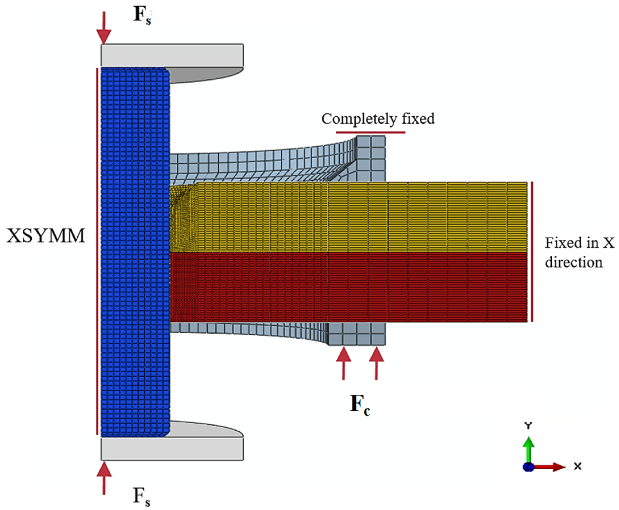
The actual riveting process included three stages of upsetting, dwelling, and unloading. The simulation model also consisted of three dynamic explicit analysis steps to replicate the above stages. The overall riveting structure was meshed using C3D8R hexahedral elements, applying reduced integration and hourglass control methods. Local mesh refinement was applied around the rivet and the hole of the connected plates, while coarser meshing was used in distant regions from the hole to reduce the number of nodes, decrease computational load, and improve efficiency. Figure 3 shows the boundary conditions of FEM. Contact relationships and mesh generation were set according to the actual riveting process.

To validate the FEM, AA2117-T4 slug rivets were installed into 2024-T351 and 7055-T76511 plates using an automated drilling–riveting cell, riveting experiments, and simulated analysis. Each configuration underwent three repeated experiments. One set of experimental and corresponding simulation results is shown in Figure 4, the numbers in the figure denote the perpendicular distance from the corresponding hole–wall locations to the central axis of the hole.

During the actual riveting process, the specimens were subjected to a riveting force of 38.4 kN and a clamping force of 19.64 MPa. Owing to the use of a quarter-symmetry FE model, the total riveting force of 38.4 kN corresponded to ~9.6 kN per symmetry sector. The rivet heads at the countersunk end were milled flat after riveting to ensure the accuracy of the aircraft profile. Therefore, the same treatment was applied in the experiments. The analysis results are shown in

Table 1. Comparison of simulated results and experimental values.

Characterization of Interference Quantity	2024-T351			7055-T76511
	Experiment (mm)	Simulation (mm)	Error (mm)	Experiment (mm)	Simulation (mm)	Error (mm)
G1	0.275	0.286	0.011	0.111	0.115	0.004
G2	0.150	0.136	0.014	0.069	0.065	0.004
G3	0.121	0.124	0.003	0.056	0.057	0.001
G4	0.217	0.219	0.002	0.103	0.094	0.009

. Dimensional calibration was performed prior to measurement, and the reported values represented the mean of three repeated tests.

For interference connection, numerous parameters affect the interference fit level. To balance predicted accuracy and computational complexity, a subset of parameters was selected for sample data preparation. The material property parameters included the elastic modulus, initial yield stress, hardening exponent, and hardening constant of the connected parts. And rivet protrusion length was included as the geometric parameter. The process parameters chosen comprised the riveting force, die dwell time, and clamping force of the pressure feet.

Subsequently, the selected process parameters were studied using the orthogonal experiment to analyze their effects on the four interference values. Additionally, a certain number of random process parameter combinations were generated to expand the sample datasets. Ranges for E, A, B, and n follow published aluminum-alloy data for aerospace plates, while the process windows for force, dwell, protrusion, and clamping were determined from the automatic drilling–riveting cell capability and prior shop-floor settings. An orthogonal array L50 (5¹¹) was employed to discretize each factor into five evenly spaced levels within these windows, and random samples was used to densify the interior for DNN training.

3.2. Orthogonal Experiment Design

In the practical application, the combinations of process parameters are critical for maintaining the stability of the riveting quality. The ranges of each process parameter are listed in

Table 2. The selected range of process parameters.

Parameter	Elastic Modulus (MPa)	Initial Yield Stress (MPa)	Hardening Constant (MPa)	Hardening Exponent
Maximum value	72,000	500	540	0.4
Minimum value	60,000	300	300	0.2
Parameter	Rivet protrusion length (mm)	Riveting force (N)	Die dwell time (s)	Clamping force (MPa)
Maximum value	5.5	9800	0.0021	21.64
Minimum value	4.5	9400	0.0009	17.64

. Each process parameter had five equidistant levels within the selected range. Therefore, an orthogonal array L50 (5¹¹) was used to design the experiments, resulting in 50 sets of data. The process parameter combinations are shown in

Table 3. Design of process parameter combinations for orthogonal experiments.

Riveting Force (N)	Die Dwell Time (s)	Rivet Protrusion Length (mm)	Clamping Force (MPa)	Elastic Modulus (MPa)	Initial Yield Stress (MPa)	Hardening Constant (MPa)	Hardening Exponent
9400	0.0009	4.5	17.64	60,000	300	300	0.2
9400	0.0012	4.75	18.64	63,000	350	360	0.25
9400	0.0015	5	19.64	66,000	400	420	0.3
9400	0.0018	5.25	20.64	69,000	450	480	0.35
9400	0.0021	5.5	21.64	72,000	500	540	0.4
9500	0.0009	4.75	19.64	69,000	500	300	0.25
9500	0.0012	5	20.64	72,000	300	360	0.3
9500	0.0015	5.25	21.64	60,000	350	420	0.35
9500	0.0018	5.5	17.64	63,000	400	480	0.4
9500	0.0021	4.5	18.64	66,000	450	540	0.2
9600	0.0009	5	21.64	63,000	450	480	0.2
9600	0.0012	5.25	17.64	66,000	500	540	0.25
9600	0.0015	5.5	18.64	69,000	300	300	0.3
9600	0.0018	4.5	19.64	72,000	350	360	0.35
9600	0.0021	4.75	20.64	60,000	400	420	0.4
9700	0.0009	5.25	18.64	72,000	400	540	0.3
9700	0.0012	5.5	19.64	60,000	450	300	0.35
9700	0.0015	4.5	20.64	63,000	500	360	0.4
9700	0.0018	4.75	21.64	66,000	300	420	0.2
9700	0.0021	5	17.64	69,000	350	480	0.25
9800	0.0009	5.5	20.64	66,000	350	480	0.3
9800	0.0012	4.5	21.64	69,000	400	540	0.35
9800	0.0015	4.75	17.64	72,000	450	300	0.4
9800	0.0018	5	18.64	60,000	500	360	0.2
9800	0.0021	5.25	19.64	63,000	300	420	0.25
9400	0.0009	4.5	20.64	72,000	450	420	0.25
9400	0.0012	4.75	21.64	60,000	500	480	0.3
9400	0.0015	5	17.64	63,000	300	540	0.35
9400	0.0018	5.25	18.64	66,000	350	300	0.4
9400	0.0021	5.5	19.64	69,000	400	360	0.2
9500	0.0009	4.75	17.64	66,000	400	360	0.35
9500	0.0012	5	18.64	69,000	450	420	0.4
9500	0.0015	5.25	19.64	72,000	500	480	0.2
9500	0.0018	5.5	20.64	60,000	300	540	0.25
9500	0.0021	4.5	21.64	63,000	350	300	0.3
9600	0.0009	5	19.64	60,000	350	540	0.4
9600	0.0012	5.25	20.64	63,000	400	300	0.2
9600	0.0015	5.5	21.64	66,000	450	360	0.25
9600	0.0018	4.5	17.64	69,000	500	420	0.3
9600	0.0021	4.75	18.64	72,000	300	480	0.35
9700	0.0009	5.25	21.64	69,000	300	360	0.4
9700	0.0012	5.5	17.64	72,000	350	420	0.2
9700	0.0015	4.5	18.64	60,000	400	480	0.25
9700	0.0018	4.75	19.64	63,000	450	540	0.3
9700	0.0021	5	20.64	66,000	500	300	0.35
9800	0.0009	5.5	18.64	63,000	500	420	0.35
9800	0.0012	4.5	19.64	66,000	300	480	0.4
9800	0.0015	4.75	20.64	69,000	350	540	0.2
9800	0.0018	5	21.64	72,000	400	300	0.25
9800	0.0021	5.25	17.64	60,000	450	360	0.3

.

3.3. Construction of DNN Model

Within the range of process parameters determined in the previous orthogonal experiment, additional samples were generated by randomly selecting and combining process parameters.

Let z denote the input factors [forming load, dwell time, protrusion, clamping force, E, A, B, n] and Y the targets [G1, G2, G3, G4] in mm. In total, 336 datasets were collected for training the DNN regression model. A part of these samples was set aside as a test set, while the remaining samples were randomly divided into training and validation sets with a 3:1 ratio. All process parameter values of the samples were normalized using Equation (2).

$$z={\displaystyle \frac{x-x_{\min }}{x_{\max }-x_{\min }}}$$

(2)

After preparation of the dataset, the problem could be abstracted into a multivariate nonlinear regression problem with eight inputs and four outputs. In this context, a DNN regression model was constructed using the PyTorch 2.1.0 [27] package in Python 3.11.5. The model consisted of an input layer, multiple hidden layers, activation functions, and an output layer, and its network structure was fully connected. To ensure the stability of the regression prediction, dropout layers were not used during the model training process. The DNN model training includes forward propagation, loss calculation, backpropagation, and parameter updates, with the parameters of each network layer being updated using an optimization method.

The ReLU was employed as activation function, and the Adam optimizer (β₁ = 0.9, β₂ = 0.999) was used with an initial learning rate 1 × 10⁻³, decaying to 1 × 10⁻⁵ via cosine schedule. The mean squared error function was chosen as the loss function. Due to the existence of multiple hidden layers in the DNN model, there was a potential risk of gradient explosion and gradient vanishing during training. When the input was greater than zero, the activation function ReLU maintained a linear relationship and kept a constant gradient in this region, which helped to mitigate the problem of gradient vanishing. Additionally, the ReLU function outputs zero for negative input values, effectively truncating gradients that exceed a certain threshold to zero, thereby helping to suppress gradient explosion. The activation function ReLU is defined as follows:

$$f(x)=\left\{\begin{array}{cc}0\hfill & x<0\\ x\hfill & x\ge 0\end{array}\right.$$

(3)

The output of each layer of DNN was as shown in Equations (4) and (5).

$$a_i^l=relu(z_i^l)$$

(4)

$$z_i^l={\displaystyle \sum _{i=1}^{n^l}{\omega }_i^l}{a}_j^{l-1}+b_i^l$$

(5)

The formulation of the mean squared error (MSE) function was in Equation (6).

$$MSE={\displaystyle \frac{1}{n}}{\displaystyle \sum _{i=1}^n(Y_i-\stackrel{\wedge }{Y_i}}{)}^2$$

(6)

The Adam algorithm is an optimization method that combines the advantages of both AdaGrad [28] and RMSProp [29], and the parameters of a neural network are optimized by adaptively adjusting the learning rate.

During the training process, additional hyperparameters were adjusted, and then the final DNN hyperparameters were determined. The network consisted of four hidden layers. Based on the number of input and output parameters, the number of neurons in each layer was 8, 16, 32, 16, 8, and 4, respectively. The mini-batch size was set to 20.

Upon completing the training, two quantitative performance metrics were introduced to evaluate the prediction accuracy of the model, namely, the mean absolute error (MAE, Equation (7)) and the coefficient of determination (R², Equation (8)). Typically, MAE was used to describe the difference between the predicted values and the actual values, assessing the model’s accuracy. R² was used to evaluate the fitting degree between the predicted values and the actual values, with values closer to 1 indicating a better fit of the predictive model.

$$MAE={\displaystyle \frac{1}{N}}{\displaystyle {\sum }_{\mathrm{i}=1}^N\left|y_{act}(i)-y_{pre}(i)\right|}$$

(7)

$$R^2={\displaystyle \frac{{\displaystyle {\sum }_{i=1}^N(y_{pre}(i)-\overline{y}}{)}^2}{{\displaystyle {\sum }_{i=1}^N{(y_{act}(i)-\overline{y})}^2}}}$$

(8)

where y_act represents the measured interference value, y_pre is the predicted interference value from the model, and N refers to the number of test samples.

3.4. GA Optimization of Riveting Process

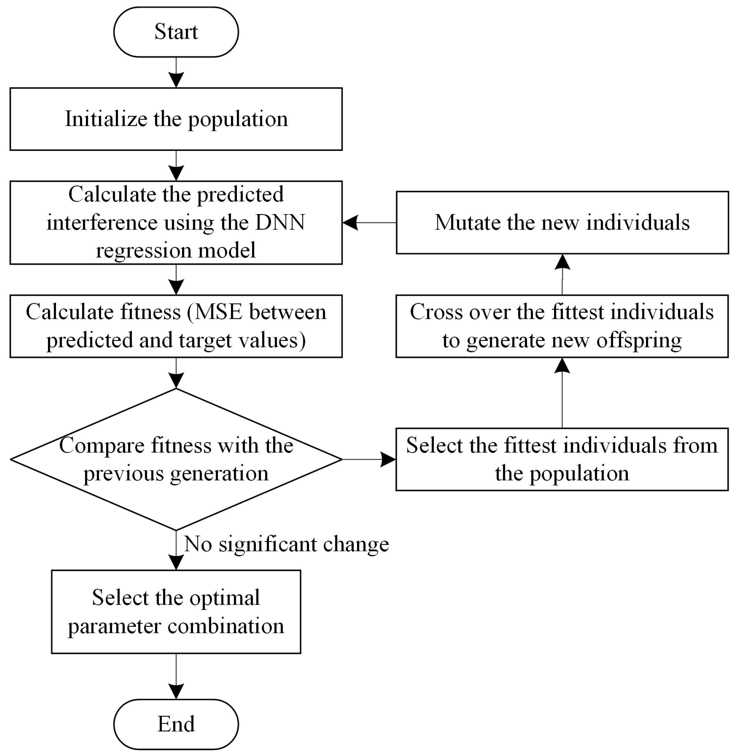
A genetic algorithm is a computational model that simulates the biological evolution process based on Darwin’s theory of natural selection and genetic mechanisms, serving as a method for searching optimal solutions by mimicking natural evolution. The specific flowchart is shown in Figure 5. By replacing the FEA calculations with a DNN model, the computational time required for GA optimization was significantly reduced.

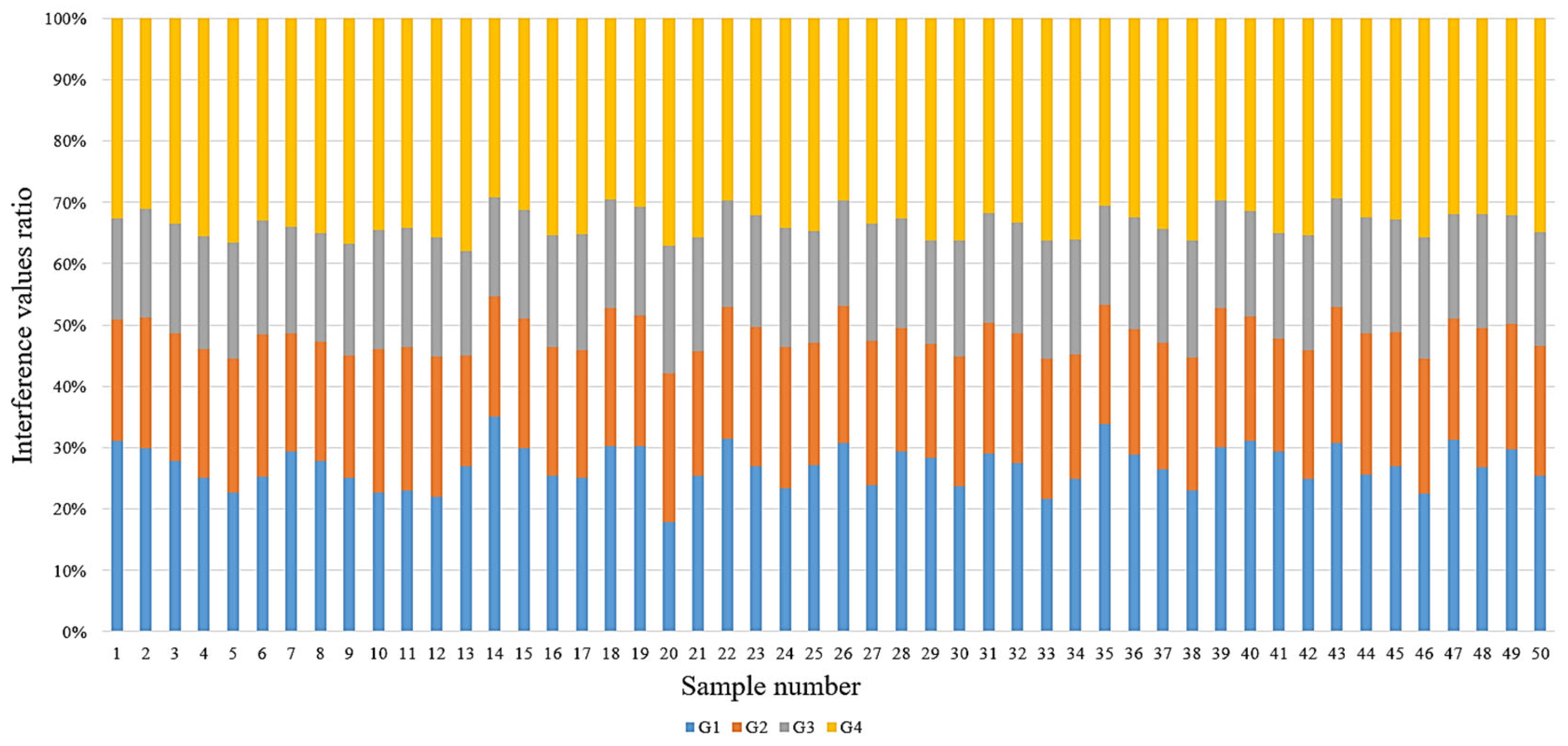
To analyze the relationships among the four interference measurements conveniently, a stacked histogram of the interference data for partial samples was created, as shown in Figure 6, which contributed to the optimization of target interference using GA.

It was observed that the ratio between the four measured interference values remained roughly constant. The average interference values for all samples are calculated and shown in

Table 4. Mean of interference values.

G1 (mm)	G2 (mm)	G3 (mm)	G4 (mm)
0.278743737	0.209038047	0.182087466	0.330130749

.

Based on the interference ratio and relevant production standards of the slug rivet, the absolute range of interference calculated for this rivet size was from 0.0488 mm to 0.1952 mm. The targeted values of interference are shown in

Table 5. Target values of interference.

Group	G1 (mm)	G2 (mm)	G3 (mm)	G4 (mm)
1	0.084	0.063	0.054	0.099
2	0.112	0.084	0.072	0.132
3	0.10	0.08	0.07	0.12

.

In practice, material property parameters are often difficult to modify, whereas process parameters such as riveting force are easily adjusted. For optimization validation, the plate material was fixed to 2024-T351 (E = 67.5 GPa, A = 330 MPa, B = 596 MPa, n = 0.52).

To obtain the desired interference value, GA was employed to optimize the process parameter combined with the pre-trained DNN prediction model. A fitness function of the optimization algorithm was constructed with the difference between the predicted results and the target interference value. The specific steps include the following four steps.

Step 1. Population Initialization: a set of individuals was initialized, and each of them contained process parameters such as riveting force, die dwell time, protrusion, and clamping force. The initial population size was set to 100.

Step 2. Fitness Calculation: combined with the material parameters of 2024-T351 aluminum alloy, the aforementioned four process parameter values of each individual were the input of the prediction model to calculate four interference values. The mean squared error between the predicted values and the targeted interference value served as the fitness function, determining the fitness score of each individual.

Step 3. Selection, Crossover, and Mutation: the fittest individuals from the population were selected, and portions of their parameter values were recombined to generate new individuals. Additionally, certain parameters of new individuals were randomly modified to generate the next generation of the population. The crossover probability and mutation probability were set as 0.5 and 0.2, respectively.

Step 4. Optimized Result Selection: The optimization procedure would terminate when there was no significant improvement in the best fitness values across the two most recent generations. Thus, the parameters of the optimal individual were selected as the final optimized result.

4. Results and Discussion

In this section, the application effect of the proposed framework on interference value prediction and process parameter optimization was discussed in detail. The influences of process parameters on the interference values were presented in Section 4.1 by orthogonal experiment results. Section 4.2 described the prediction accuracy of the constructed DNN model and its comparison with three other traditional regression models. The optimized results of the process parameter with a GA based on the DNN model were shown in Section 4.3.

4.1. Analysis of Orthogonal Test Result

Based on an orthogonal experimental design, a parametric modeling approach was developed to construct the FEM for various combinations of process parameters. Simulations were then performed to obtain the simulated values of four interference fits for each group. The simulated results are shown in Figure 7. After investigating the magnitudes of the interference values at the above four points, it was found that the interference fit levels (G1 and G4) around the rivet head were greater than the other two positions (G2 and G3). The above phenomenon could be explained as the result of the material flow of the slug rivet during the riveting process. In the initial stage, the protruding parts of the rivet shank at the top and bottom underwent plastic deformation, with most of the materials flowing into the rivet hole. Once the rivet head made contact with the connected plate, further material flow into the hole was restricted, resulting in larger interference values near the rivet head.

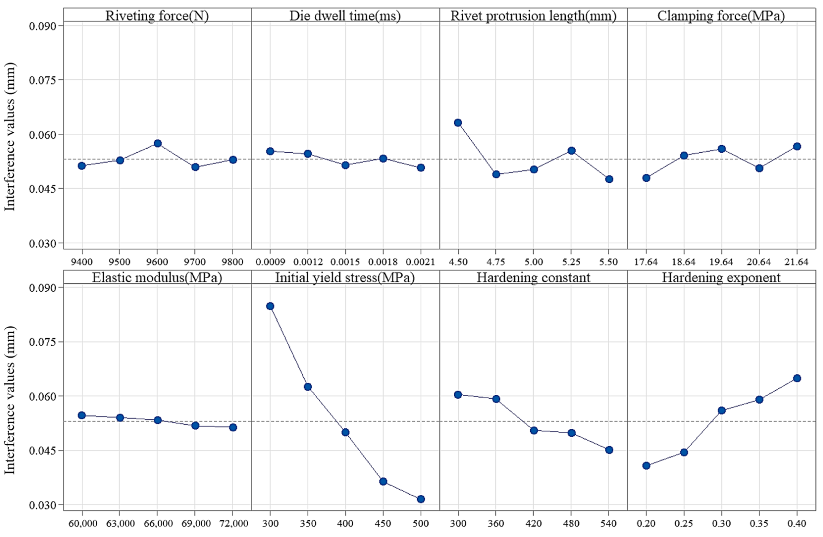
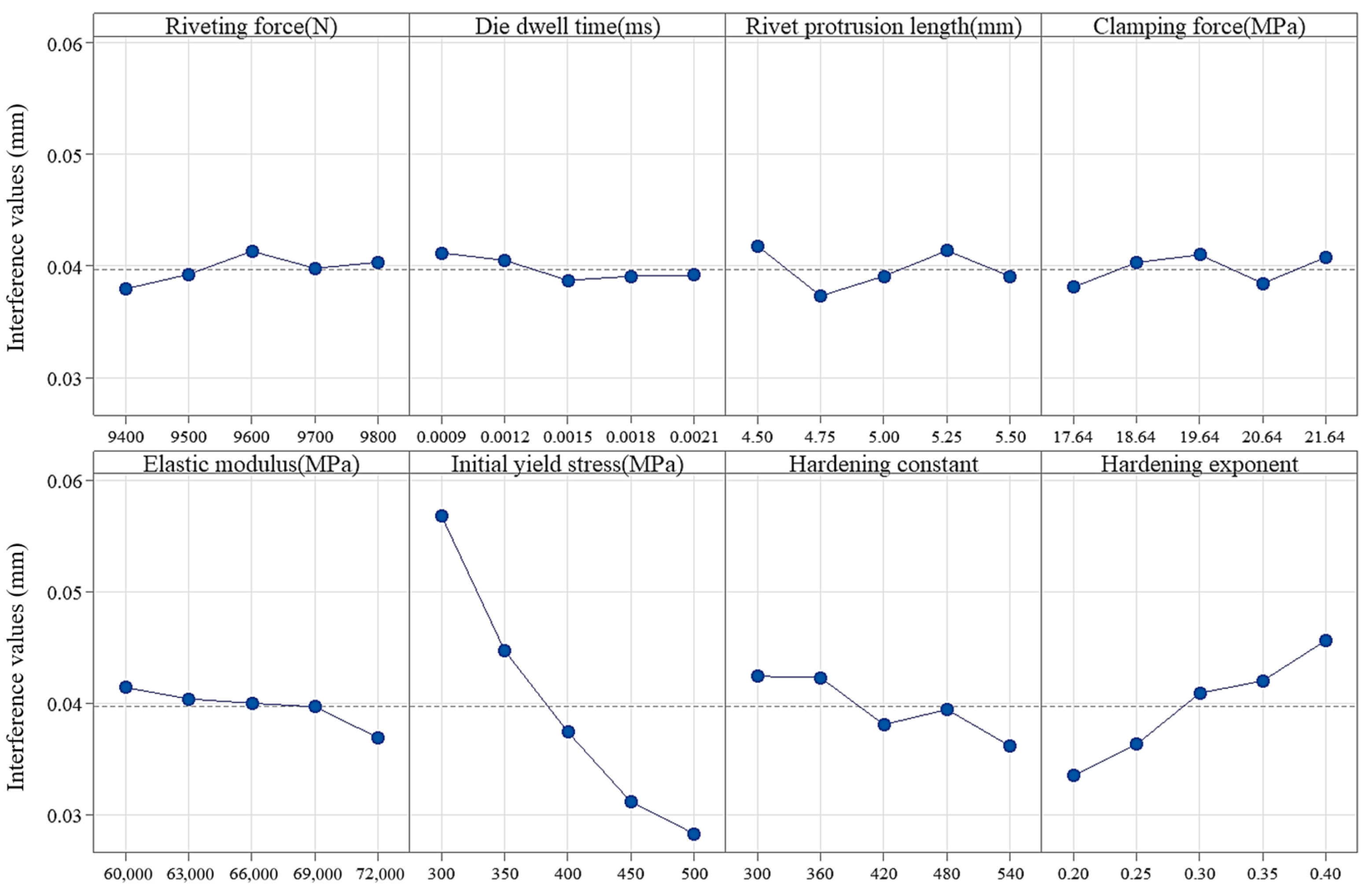
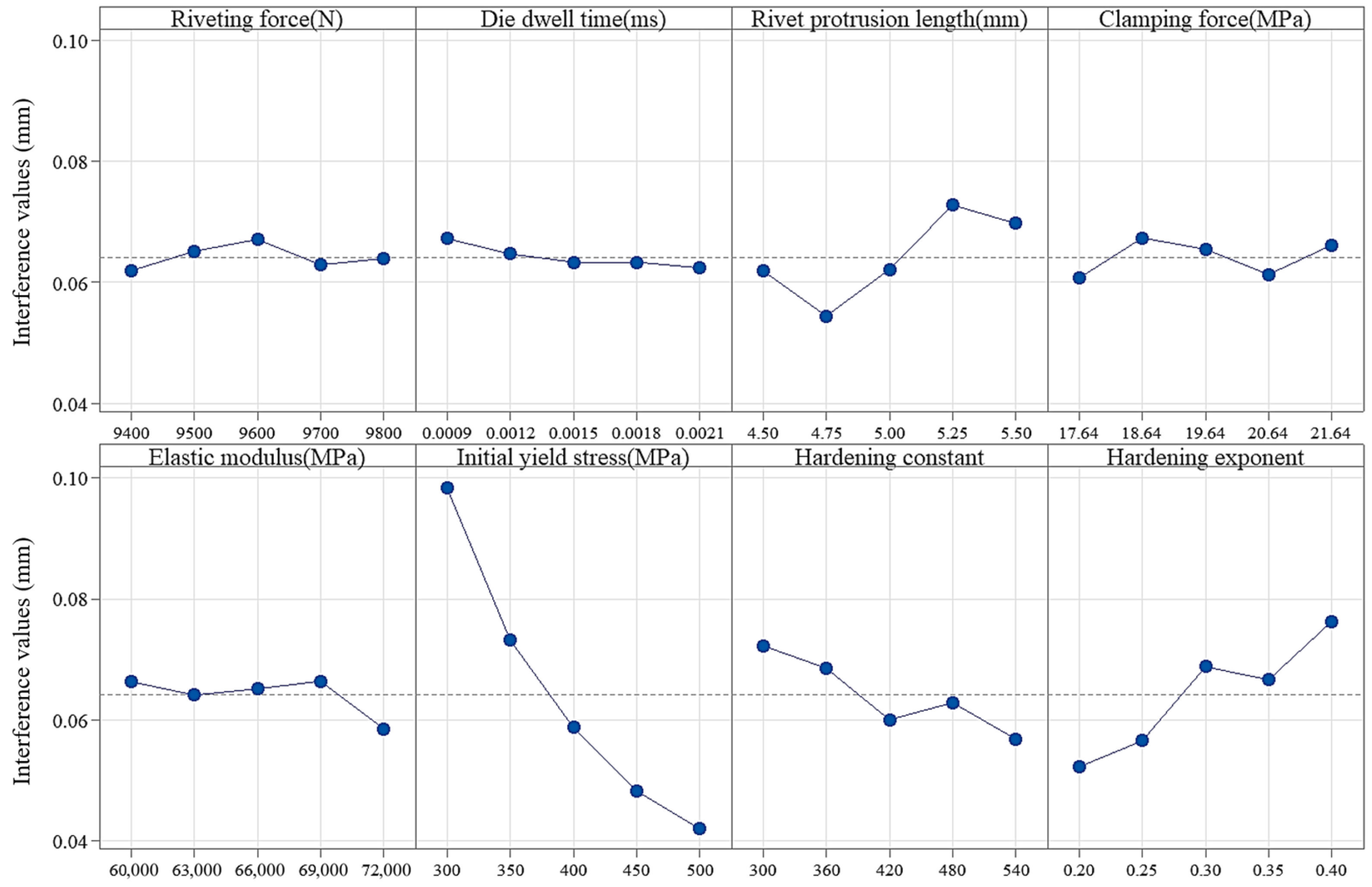
A range analysis was performed on the above data to evaluate the relative influence of each process parameter on G1, G2, G3, and G4 with Minitab 21 software. The results of the range analysis are presented in

Table 6. Range analysis of an orthogonal experiment.

Parameter	R (G1)/mm	R (G2)/mm	R (G3)/mm	R (G4)/mm	R (Average)/mm
Riveting force	0.00656	0.00338	0.00321	0.00519	0.004585
Die dwell time	0.00462	0.00246	0.00216	0.00485	0.0035225
Rivet protrusion length	0.01554	0.00449	0.00612	0.01836	0.0111275
Clamping force	0.00872	0.00290	0.00272	0.00665	0.0052475
Elastic modulus (E)	0.00324	0.00451	0.00440	0.00789	0.00501
Initial yield stress (A)	0.05321	0.02852	0.02701	0.05644	0.041295
Hardening constant (B)	0.01523	0.00628	0.00571	0.01545	0.0106675
Hardening exponent (n)	0.02413	0.01216	0.01138	0.02409	0.01794

, while Figure 8, Figure 9, Figure 10 and Figure 11 show the impact trend of each factor on the interference. A steeper slope of the trend curve indicated a greater impact of the factor on the interference. As shown in Table 6, it is observed that the range values of yield strength A are the largest for G1, G2, G3, and G4. The range values of elastic modulus E were the minimum, which indicated that the yield stress has the greatest impact on the interference fit level of the slug rivet, whereas the elastic modulus has the least impact. The ranking of factors by their influence was as follows: initial yield stress > hardening exponent > hardening constant > elastic modulus.

Initial yield stress A had the largest influence on the riveting interference, followed by the hardening exponent n, while elastic modulus E and hardening constant B had similar effects. The hardening exponent n was positively correlated with the riveting interference value, whereas the initial yield stress A was negatively correlated. According to the riveting process, the slug rivet was deformed under riveting force, then the riveting shank expanded the rivet hole, namely, the interference was primarily driven by the plastic deformation of the rivet. When the rivet is subjected to a certain riveting force, the initial yield stress of the connected plates determines the degree of deformation difficulty. The higher yield strength of connected plates results in a more difficult deformation occurring, which results in a smaller interference.

Considering the properties of the exponential function in the Johnson–Cook constitutive model [30], a larger value of n resulted in less sensitivity to increases in εⁿ, and the function grows more gradually within the limits of 0 to 1. Therefore, under a given riveting force, a larger n led to greater strain in the plastic stage, which increased the interference in turn.

In the range analysis, it could be concluded that the variation in protrusion length had the greatest effect on the G1 and G4. The increase in protrusion strengthened the compression of the lower half of the hole wall during the riveting process, leading to significant changes in G4. Similarly, the increase in protrusion also had the same influence on the upper half of the hole wall through plastic flow of material, which resulted in an increased interference at other locations. Additionally, an increase in clamping force and riveting force also enhanced the material flow and deformation, thereby increasing the interference fit level. It was interesting that an extension in dwell time of riveting force led to a certain reduction in interference, possibly because of the occurrence of stress relaxation under high-stress conditions if the riveting force was applied for a prolonged period [31,32]. The stress relaxation reduced the generated residual stress during the deformation process, ultimately leading to a decrease in the interference to some extent. From the above range analysis, it was evident that G1 and G4, which were less constrained compared to the middle regions G2 and G3 of the rivet hole wall, presented a greater change in interference value when process parameters were varied.

The larger response of G1 and G4 to protrusion reflects directional material flow at early upsetting, where shank expansion was constrained by head–plate contact. The observed decrease with prolonged dwell was consistent with stress-relaxation under high contact stress, effectively reducing retained interference. These trends supported the factor ranking and explained why edge-adjacent gauges (G1, G4) are more sensitive than mid-wall gauges (G2, G3).

In summary, it was obvious that each selected process parameter has a certain degree of influence on the interference fit level of the slug rivet. The rationality and effectiveness of each process parameter as an input of the DNN regression prediction model have also been demonstrated.

4.2. Verification of DNN Model Prediction Performance

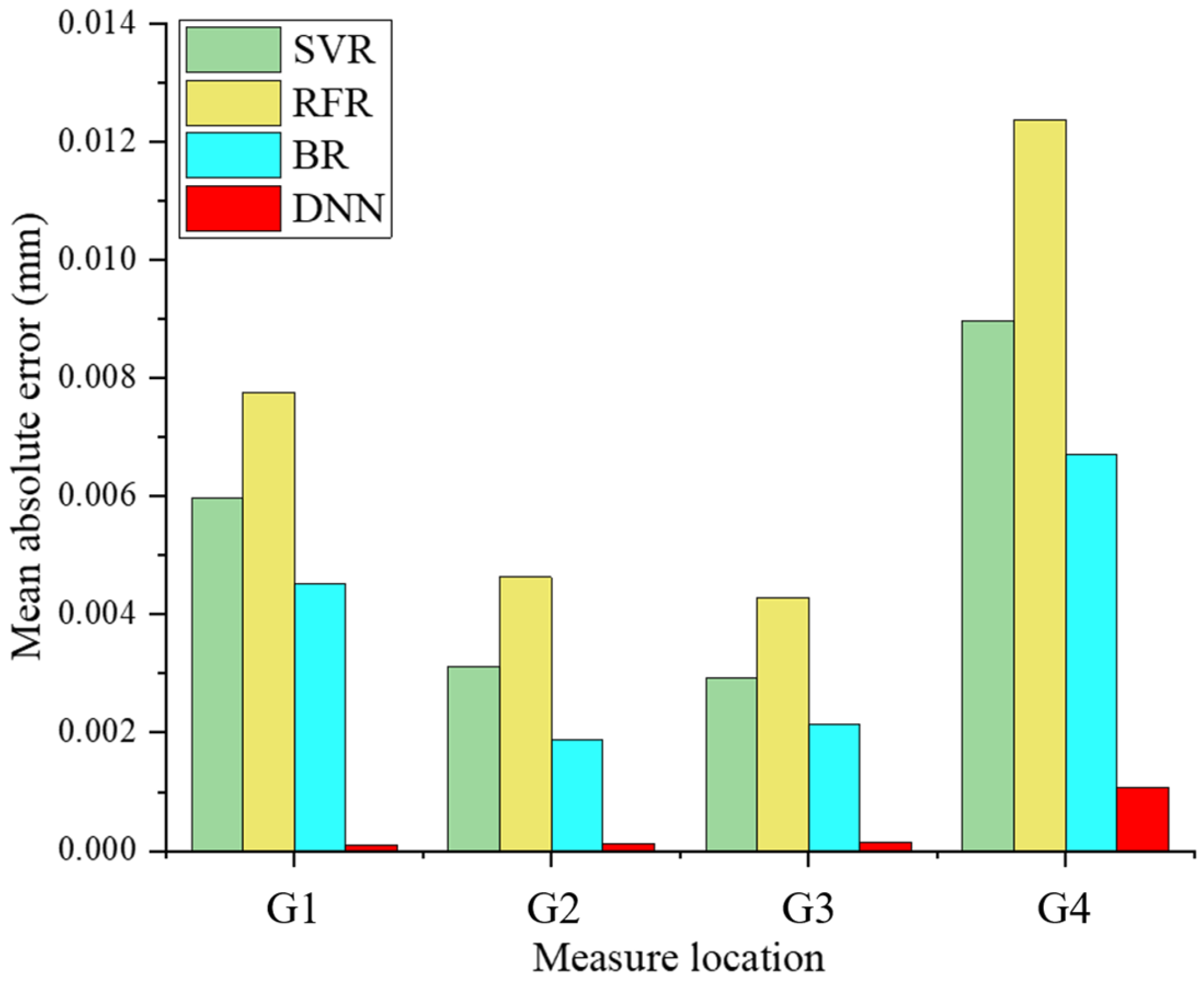
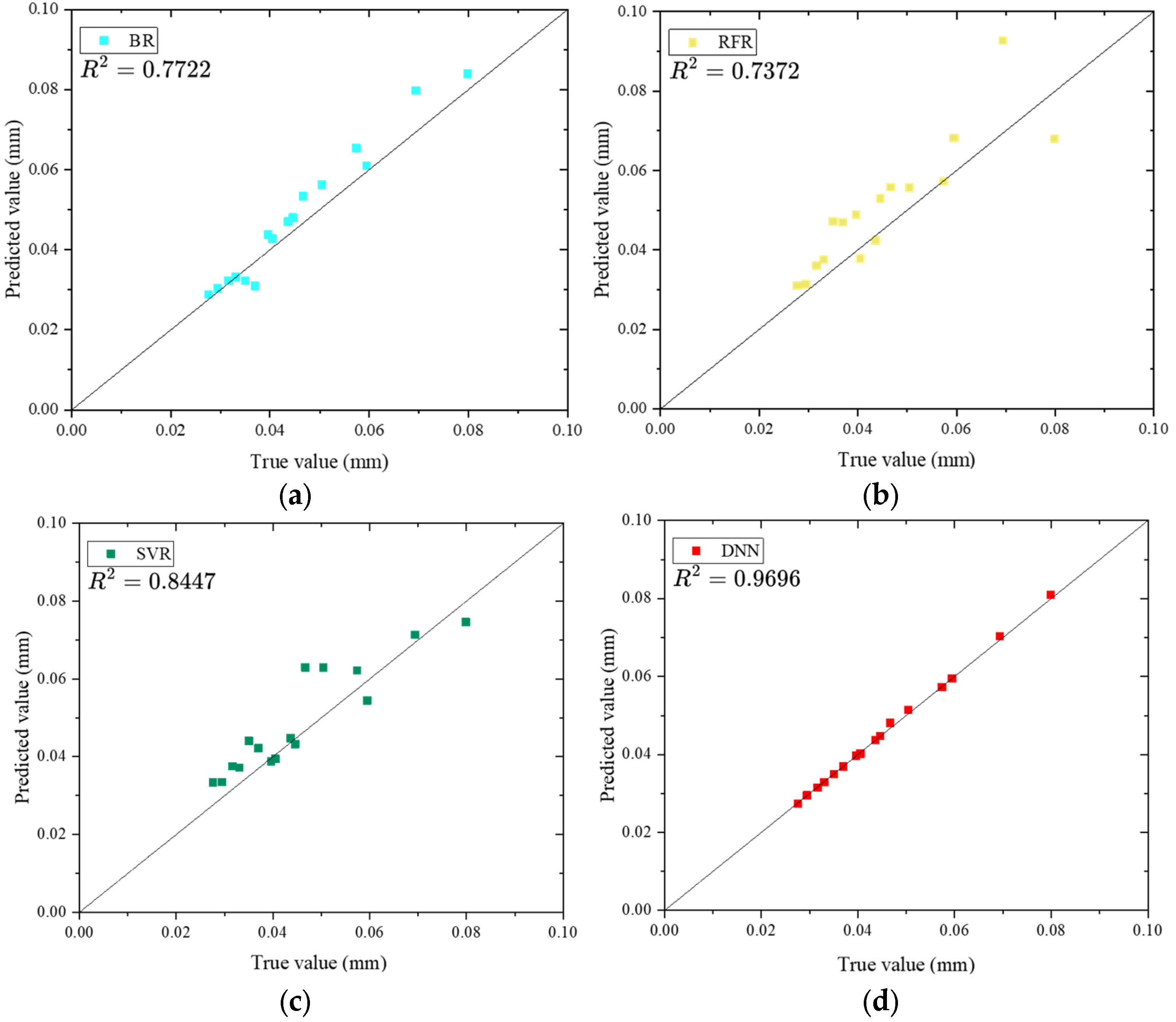
To verify the superiority and accuracy of the DNN regression model, three other data-driven regression models were established with the same dataset, including Support Vector Regression (SVR), Random Forest Regression (RFR), and Bayesian Regression (BR). To assess the prediction performance quantitatively, the same test dataset was used to calculate the Mean Absolute Error (MAE) and the coefficient of determination (R²) for each regression model. The results are illustrated in Figure 12 and Figure 13.

As illustrated in Figure 13, the DNN model exhibits the smallest relative error in the test set and achieves the best fitting performance. The MAE for all test set samples was 0.00035 mm, with a mean relative error of 0.72%. Compared to three other traditional regression models, the DNN model demonstrated a clear advantage and effectiveness in serving as a substitute for the finite element simulation model.

Interference in slug-rivet joints emerges from coupled, non-separable interactions among load, dwell, protrusion, clamping, and plasticity parameters. A DNN with ReLU layers provides a high-capacity, adaptive basis that captures high-order cross-factor interactions and smooth, monotone trends within the design window. In contrast, SVR with a single stationary kernel imposes a few global length scales, which underfits anisotropic factor sensitivities and either over- or under-smooths regimes with different curvature; Random-Forest regression yields piecewise-constant predictors that bias continuous interference responses and degrade near extrema; and Bayesian regressors lack expressive nonlinearity and scale poorly with sample size while remaining constrained by stationarity assumptions. The DNN also supports multi-output learning via a shared trunk and four output heads, allowing G1–G4 to share latent structure and improving data efficiency.

4.3. Optimized Results of Process Parameters

Embed the DNN into the GA as a surrogate for the FEM, yielding a DNN-enhanced GA optimization model. After iterative optimization with DNN-enhanced GA, the optimized process parameters for each group are shown in

Table 7. Combination of process parameters after GA optimization.

Group	Riveting Force (N)	Die Dwell Time (s)	Rivet Protrusion Length (mm)	Clamping Force of the Pressure Feet (MPa)
1	9869.440	0.00098496	5.1256	21.1568
2	10,002.356	0.00035664	4.508316	18.3692
3	9964.080	0.00060456	4.7575	17.63762

.

Combined with previous material parameters, the optimized process parameters were used to establish an FEA model. Then, the interference values were calculated and compared with the targeted interference values. The comparative results are listed in

Table 8. Comparison between the optimal value and the targeted value.

	Interferometric Measurement Position	Optimal Values (mm)	Targeted Values (mm)	Relative Deviation
1	G1	0.090707899	0.084	7.99%
	G2	0.066179493	0.063	5.05%
	G3	0.0591217	0.054	9.48%
	G4	0.105208	0.099	6.27%
2	G1	0.121151878	0.112	8.17%
	G2	0.083218121	0.084	0.93%
	G3	0.0693104	0.072	3.74%
	G4	0.124837	0.132	5.43%
3	G1	0.104535649	0.10	4.54%
	G2	0.074297139	0.08	7.13%
	G3	0.0631781	0.07	9.75%
	G4	0.111384	0.12	7.18%

.

As shown in Table 8, the results reveals that the interference values obtained using the optimized process parameters closely matches the targeted interference values, with a maximum relative error of 9.75%, which demonstrates the effectiveness of the proposed optimization method.

A single FEM run for data generation required over 60 min on a workstation, whereas DNN inference for a single candidate took < 1 s. Given that the GA evaluated 10²–10³ candidates per generation, replacing FEM with DNN reduced the computational cost per generation by three to four orders of magnitude. The novelty lies in a validated FEM→DNN→GA loop with factor-ranking and target-seeking interference control, delivering minute-scale optimization while retaining physical interpretability via range analysis and partial dependence.

5. Conclusions

This paper presented an interference value prediction and optimization framework for slug rivets, employing a method based on DNN-enhanced GA to optimize the riveting process parameters. By combining the finite element simulation with an intelligent algorithm, the optimized process parameters for the targeted interference fit level were acquired. The following conclusions could be drawn:

(1)

A parametric finite element model for the riveting process of the slug rivet was established and subsequently validated through experiments. The verification demonstrated that the constructed FE model could predict riveting interference value accurately.

(2)

Orthogonal experiments were designed to investigate the effect of riveting parameters on the interference value. It was found that the initial yield stress of the connected plates had the most significant influence.

(3)

A regression prediction model based on DNN was proposed, and its predicted results were compared with three other traditional regression models (support vector machine regression, random forest regression, and Bayesian regression). The results showed that the proposed DNN regression model revealed a superior capability for fitting the multivariate nonlinear relationship between riveting process parameters and the interference value, which achieved a determination coefficient R-squared of 0.9696 and a mean absolute error of 0.00035 mm.

(4)

The riveting process parameters were optimized with a DNN-enhanced GA algorithm. Compared with simulated results, the target interference value showed a maximum relative error of 9.75%.

References

1. Wang, Z.; Chang, Z.; Guo, F.; Kang, Y.; Li, H.; Luo, Q.; Liu, B. Interference-Fit slug Rivet Joining Technology for Large-Aircraft Skin Panels. Aeronaut. Manuf. Technol. 2015, 34–39. [Google Scholar] [CrossRef]
2. Liu, L.; Li, X.; Wang, Z.; Li, W. Experimental Investigation of an Automated Drilling-Riveting Process for slug Rivets. J. Northwestern Polytech. Univ. 2013, 31, 77–82. [Google Scholar]
3. Lei, C.; Bi, Y.; Li, J.; Ke, Y. Experiment and Numerical Simulations of a Slug Rivet Installation Process Based on Different Modeling Methods. Int. J. Adv. Manuf. Technol. 2018, 97, 1481–1496. [Google Scholar] [CrossRef]
4. Lv, G.; Li, C.; Zhao, C.; Jia, D.; Zhang, X.; Zhang, H.; Huang, W. Research on Theoretical Prediction Method of Rivet-Forming Quality Considering Different Riveted Structure Parameters. Int. J. Adv. Manuf. Technol. 2024, 132, 2333–2345. [Google Scholar] [CrossRef]
5. Liang, Q.; Zhang, T.; Zhu, C.; Bi, Y. Effect of Riveting Angle and Direction on Fatigue Performance of Riveted Lap Joints. Coatings 2021, 11, 236. [Google Scholar] [CrossRef]
6. Tian, S.; Li, C.; Dai, W.; Jia, D.; Zhang, H.; Xu, M.; Yuan, Y.; Liu, Y.; Zhang, Y. Effect of the Countersunk Hole Depth on Tensile-Tensile Fatigue Behavior of Riveted Specimens of AA2024-T3 Alloy. Eng. Fail. Anal. 2020, 115, 104639. [Google Scholar] [CrossRef]
7. Derijck, J.; Homan, J.; Schijve, J.; Benedictus, R. The Driven Rivet Head Dimensions as an Indication of the Fatigue Performance of Aircraft Lap Joints. Int. J. Fatigue 2007, 29, 2208–2218. [Google Scholar] [CrossRef]
8. Huang, L.; Shi, Y.; Guo, H.; Su, X. Fatigue Behavior and Life Prediction of Self-Piercing Riveted Joint. Int. J. Fatigue 2016, 88, 96–110. [Google Scholar] [CrossRef]
9. Casolaro, A.; Capone, V.; Iannuzzo, G.; Camastra, F. Deep Learning for Time Series Forecasting: Advances and Open Problems. Information 2023, 14, 598. [Google Scholar] [CrossRef]
10. Yang, G.R.; Wang, X.-J. Artificial Neural Networks for Neuroscientists: A Primer. Neuron 2020, 107, 1048–1070. [Google Scholar] [CrossRef]
11. LeCun, Y.; Bengio, Y.; Hinton, G. Deep Learning. Nature 2015, 521, 436–444. [Google Scholar] [CrossRef]
12. Belhouchet, K.; Bayadi, A.; Bendib, M.E. Artificial Neural Networks (ANN) and Genetic Algorithm Modeling and Identification of Arc Parameter in Insulators Flashover Voltage and Leakage Current. In Proceedings of the 2015 4th International Conference on Electrical Engineering (ICEE), Boumerdes, Algeria, 13–15 December 2015; pp. 1–6. [Google Scholar]
13. Wang, Z.; Jia, Y.; Fu, P.; Li, H.; Song, L.; Yang, B.; Zhang, L.; Yuan, L.; Shi, K. Research on the Online Evaluation of the Straightness Error of Hydrostatic Guideways Based on Deep Learning. Int. J. Adv. Manuf. Technol. 2024, 134, 2023–2034. [Google Scholar] [CrossRef]
14. Deshpande, S.; Venugopal, V.; Kumar, M.; Anand, S. Deep Learning-Based Image Segmentation for Defect Detection in Additive Manufacturing: An Overview. Int. J. Adv. Manuf. Technol. 2024, 134, 2081–2105. [Google Scholar] [CrossRef]
15. Sun, H.; Cui, J.; Li, G.; Jiang, H. Genetic Sampling for Surrogate-Assisted Topology Optimization in Electromagnetic Riveting Device Design. Mater. Des. 2024, 237, 112527. [Google Scholar] [CrossRef]
16. Masoudi Nejad, R.; Sina, N.; Ma, W.; Song, W.; Zhu, S.P.; Branco, R.; Macek, W.; Gholami, A. Artificial Neural Network Based Fatigue Life Assessment of Riveted Joints in AA2024 Aluminum Alloy Plates and Optimization of Riveted Joints Parameters. Int. J. Fatigue 2024, 178, 107997. [Google Scholar] [CrossRef]
17. Michalewicz, Z.; Schoenauer, M. Evolutionary Algorithms for Constrained Parameter Optimization Problems. Evol. Comput. 1996, 4, 1–32. [Google Scholar] [CrossRef]
18. Tomar, V.; Bansal, M.; Singh, P. Metaheuristic Algorithms for Optimization: A Brief Review. In Proceedings of the RAiSE-2023, Dubai, United Arab Emirates, 13 March 2024; p. 238. [Google Scholar]
19. Shi, S.; Cheng, W.; Wang, Z. Intelligent Rivet Selection Technology for Interference-Fit Magnitude Control. Aeronaut. Manuf. Technol. 2021, 64, 74–79+85. [Google Scholar] [CrossRef]
20. Choudhary, A.; Kumar, M.; Gupta, M.K.; Unune, D.K.; Mia, M. Mathematical Modeling and Intelligent Optimization of Submerged Arc Welding Process Parameters Using Hybrid PSO-GA Evolutionary Algorithms. Neural Comput. Appl. 2020, 32, 5761–5774. [Google Scholar] [CrossRef]
21. Rajendran, S.; Ganesh, N.; Čep, R.; Narayanan, R.C.; Pal, S.; Kalita, K. A Conceptual Comparison of Six Nature-Inspired Metaheuristic Algorithms in Process Optimization. Processes 2022, 10, 197. [Google Scholar] [CrossRef]
22. Ni, J.; Tang, W.C.; Xing, Y. Assembly Process Optimization for Reducing the Dimensional Error of Antenna Assembly with Abundant Rivets. J. Intell. Manuf. 2018, 29, 245–258. [Google Scholar] [CrossRef]
23. Wu, P.; He, Y.; Li, Y.; He, J.; Liu, X.; Wang, Y. Multi-Objective Optimisation of Machining Process Parameters Using Deep Learning-Based Data-Driven Genetic Algorithm and TOPSIS. J. Manuf. Syst. 2022, 64, 40–52. [Google Scholar] [CrossRef]
24. Da Costa Oliveira, A.L.; Britto, A.; Gusmão, R. Machine Learning Enhancing Metaheuristics: A Systematic Review. Soft Comput. 2023, 27, 15971–15998. [Google Scholar] [CrossRef]
25. Demmel, F.; Hennet, L.; Jakse, N. The Intimate Relationship between Structural Relaxation and the Energy Landscape of Monatomic Liquid Metals. Sci. Rep. 2021, 11, 11815. [Google Scholar] [CrossRef]
26. Li, X.; Chang, Z.; Gao, Y.; Huo, Y.; Song, J.; Wang, Z. Prediction of slug Rivet Interference-Fit Magnitude Using a Multivariate Nonlinear Regression Model. J. Xi’an Jiaotong Univ. 2024, 58, 157–166. [Google Scholar]
27. Novac, O.-C.; Chirodea, M.C.; Novac, C.M.; Bizon, N.; Oproescu, M.; Stan, O.P.; Gordan, C.E. Analysis of the Application Efficiency of TensorFlow and PyTorch in Convolutional Neural Network. Sensors 2022, 22, 8872. [Google Scholar] [CrossRef]
28. Tian, Y.; Zhang, Y.; Zhang, H. Recent Advances in Stochastic Gradient Descent in Deep Learning. Mathematics 2023, 11, 682. [Google Scholar] [CrossRef]
29. Hong, D.; Chen, D.; Zhang, Y.; Zhou, H.; Xie, L. Attacking Robot Vision Models Efficiently Based on Improved Fast Gradient Sign Method. Appl. Sci. 2024, 14, 1257. [Google Scholar] [CrossRef]
30. Kumar, H.; Manna, R.; Khan, D. Evaluation of Johnson–Cook Material Model Parameters for Fe–30Mn–9Al–0.8C Low-Density Steel in Metal Forming Applications. J. Mater. Sci. 2023, 58, 8118–8129. [Google Scholar] [CrossRef]
31. Li, M.; Liu, Z.; Huang, L.; Chen, Q.; Tong, C.; Fang, Y.; Han, W.; Zhu, P. Automatic Identification Framework of the Geometric Parameters on Self-Piercing Riveting Cross-Section Using Deep Learning. J. Manuf. Process. 2022, 83, 427–437. [Google Scholar] [CrossRef]
32. Zhu, J.; Yuan, W.; Peng, F.; Fu, Q. Interaction of Stress Relaxation Aging Behavior and Microstructural Evolution in Inconel 718 Alloy with Different Initial Stress Status. J. Mater. Sci. 2021, 56, 13814–13826. [Google Scholar] [CrossRef]
Figure 1. Flowchart of riveting process parameters optimization.
Machines 13 00936 g001
Figure 2. The specific measurement position of riveting interference quantity.
Machines 13 00936 g002
Figure 3. Boundary condition setting of FEM.
Machines 13 00936 g003
Figure 4. Comparison between the experimental results and the simulation results [26].
Machines 13 00936 g004
Figure 5. Flowchart of process parameter optimization.
Machines 13 00936 g005
Figure 6. Stacked histogram of samples.
Machines 13 00936 g006
Figure 7. Partial simulation results of the orthogonal experiment.
Machines 13 00936 g007
Figure 8. Influence trend on the interference fit of G1.
Machines 13 00936 g008
Figure 9. Influence trend on the interference fit of G2.
Machines 13 00936 g009
Figure 10. Influence trend on the interference fit of G3.
Machines 13 00936 g010
Figure 11. Influence trend on the interference fit of G4.
Machines 13 00936 g011
Figure 12. MAE of each regression model (mm).
Machines 13 00936 g012
Figure 13. Prediction fitting performance of each model. (a) Bayesian regression, (b) Random forest regression, (c) Support vector machine regression, (d) DNN model.
Machines 13 00936 g013