Abstract
In disturbance scenarios, wheeled bipedal robots (WBRs) require effective control algorithms to restore balance. To address the trade-off between computational burden and control precision, and to enhance anti-disturbance capability, this paper proposes a soft-constrained Model Predictive Control (MPC) algorithm with optimized horizon parameters tailored to the hardware of the WBR. A cost function is designed, and the Dung Beetle Optimizer (DBO) is employed to optimize the MPC’s prediction and control horizons. An experimental platform is built, and impact and load disturbance experiments are conducted. The experimental results show that, under impact disturbances, the pitch angle and displacement overshoot with optimized MPC are reduced by 58.57% and 42.20%, respectively, compared to unoptimized LQR. Under load disturbances, the pitch angle and displacement overshoot are reduced by 17.09% and 15.53%, respectively, with both disturbances converging to the equilibrium position.
1. Introduction
In the field of mobile robotics, wheeled bipedal robots (WBRs) combine the advantages of humanoid and wheeled robots. They use leg structures to isolate torso vibrations caused by terrain irregularities, while employing wheels for balance and dynamic motion, making them well-suited for human working environments [1]. However, in typical working environments, WBRs are frequently subject to various types of disturbances, leading to issues such as slow control response, insufficient vibration suppression, overshoot, or oscillations, which negatively affect their performance [2]. Therefore, it is essential to design an anti-disturbance balance control algorithm that ensures control precision under limited computational resources, further enhancing the anti-disturbance performance of WBRs.
For WBRs, balance capability and anti-disturbance performance are fundamental for executing other actions. Traditional balance control methods can achieve basic balance control for WBRs, such as Proportional–Integral–Derivative (PID), Linear Quadratic Regulator (LQR), and Zero-Moment Point (ZMP) methods. These methods typically simplify the WBR to a Linear Inverted Pendulum (LIP) by ignoring leg dynamics to achieve balance control [3]. Appropriate control algorithms can also be obtained through model reduction methods. A reduced-order model based on the Cuckoo Search Algorithm can reduce the computational burden of balance control [4]. In nonlinear domains that cannot be simplified, balance control can be achieved using the State-Dependent Riccati Equation (SDRE) control algorithm [5]. For WBRs with complex structures and state-space equations that are difficult to solve, Reinforcement Learning (RL) and Adaptive Dynamic Programming (ADP) can be employed to provide adaptive optimal control solutions based on learning [6]. For WBRs with known state-space equations, LQR can effectively achieve balance control with highly efficient performance [7]. However, the gain coefficients of the aforementioned control algorithms are mostly fixed, resulting in limited real-time responsiveness when the robot’s external environment changes.
When the system model is known and the main control device has sufficient computational power, Model Predictive Control (MPC) can be effectively used for state tracking of the model. Thanks to the “online” feature of MPC, the algorithm can update the planned trajectory within the feedback loop at a certain frequency, providing the robot with enhanced robustness against disturbances [8]. Additionally, MPC can incorporate various inequality constraints, enhancing the system’s insensitivity to external disturbances [9].
The original MPC method can effectively achieve anti-disturbance balance control for WBRs. A control algorithm is designed based on the robot’s state-space model and formulated as a quadratic programming problem, yielding optimal outputs for given prediction and control horizons. In certain scenarios, this method achieves minimal control efforts superior to those of the LQR algorithm [10]. Shahida Khatoon et al. [11] applied MPC with Linear Quadratic Gaussian Controller (LQG) to a wheeled inverted pendulum system and conducted impact tests, with simulation results showing that MPC exhibits strong robustness. Yu Jianqiao et al. [12] applied MPC to the posture control of a WBR, ensuring that the robot tracks the posture trajectory with minimal error and maintains balance. Niloufar Minouchehr et al. [13] treated a two-wheeled inverted pendulum as an underactuated nonlinear system and designed an MPC algorithm to achieve anti-disturbance control. Marco Kanneworff et al. [14] developed an Intrinsically Stable MPC (IS-MPC) algorithm, achieving stable control of an arm-equipped wheeled inverted pendulum robot under explicit constraints. Cao Haixin et al. [15] designed a constrained MPC algorithm to achieve balance control for a WBR on sloped terrains and enhanced the robustness of the control algorithm by developing an Extended State Observer (ESO). These methods applied MPC to WBRs and achieved balance control; however, they did not constrain system states and control inputs based on the robot’s hardware performance. This oversight could lead to inaccuracies in the MPC’s computed results, rendering the robot uncontrollable due to hardware power limitations. In particular, when the robot is subjected to disturbances, the driving wheel motors often need to output large torques within a short time to maintain balance. However, if the motors operate beyond their rated torque for extended periods, issues such as control delays, overheating, and performance degradation may occur. Unlike hard constraints, which may render the optimization problem infeasible under large disturbances, soft constraints introduce a penalty mechanism that tolerates minor violations. This design ensures the continuous feasibility of the controller while balancing constraint satisfaction and control performance, thereby enhancing robustness and practicality in real-world applications. By introducing soft constraints into the MPC framework, the range of control inputs can be effectively limited, ensuring that the control signals remain within the rated torque and below the peak torque. This not only protects the hardware from overload but also enhances the feasibility and anti-disturbance performance of the control algorithm. To enhance the effectiveness of MPC in practical applications, researchers have proposed various methods to optimize control performance. Daniel C. Fernández et al. [16] conducted simulation experiments with multiple prediction horizons, achieving the control objectives of reducing control errors and ensuring computational speed. Li Xingjia et al. [17] employed the Transient Search Optimization (TSO) algorithm to optimize the parameters of the MPC objective function, reducing the overshoot and steady-state error of the controlled robot. A. K. Kashyap et al. [18] combined the Ant Colony Optimization (ACO) algorithm with MPC to optimize the robot’s position-solving problem in obstacle scenarios. Chen Zhenbin et al. [19] applied the Proximal Policy Optimization (PPO) learning method to adaptively adjust the prediction range within the MPC framework, achieving stable trajectory tracking. Jin Mengtao et al. [20] used the Chaos Particle Swarm Optimization (CPSO) algorithm to optimize the solving capability of MPC, effectively improving trajectory tracking performance. These methods optimized MPC parameters for various target scenarios applied to robots, improving the tracking performance of target state variables. However, the optimized parameters were relatively limited, and the considered scenarios did not comprehensively account for disturbances. For WBRs with high real-time response requirements, the sizes of the MPC’s prediction and control horizons affect both the computation of control outputs and the main control device’s computation time [21]. Among common heuristic optimization algorithms, the Dung Beetle Optimizer (DBO) algorithm proposed by Xue Jiankai et al. [22] can achieve multi-objective optimization and solutions. Yang Pei et al. [23] applied DBO to solve the optimization model for lightweight objectives, obtaining a global optimal solution with fewer iterations. Li Yanhui et al. [24] applied DBO to optimize wind models, obtaining an optimal set of model parameters. Due to its powerful solution space exploration capability, DBO outperforms classic optimization algorithms such as PSO [25].
Therefore, this paper proposes a soft-constrained MPC algorithm tailored to the hardware specifications of WBRs and optimizes the combination of prediction and control horizons for different disturbance scenarios, further enhancing the robot’s stability under disturbances. The main contributions of this paper are as follows:
- (1)
- To address the problem of anti-disturbance control for WBRs, a soft-constrained MPC algorithm considering hardware power limitations is proposed to optimize the feasible domain of control outputs.
- (2)
- The domain parameters of the MPC algorithm are optimized using the heuristic DBO algorithm, reducing the computation time of the main control device while ensuring the robot’s anti-disturbance performance.
- (3)
- An SRobo110-II experimental platform and disturbance equipment are constructed to validate the proposed method through comparisons with the LQR balance control algorithm and others.
Besides this section, the structure of this paper is as follows: Section 2 establishes the dynamic model of the WBR through Newtonian mechanics analysis. Section 3 designs the MPC algorithm, sets reasonable control constraints based on the robot’s hardware, and optimizes the sizes of the MPC’s prediction and control horizons using the heuristic DBO algorithm. Section 4 constructs the experimental platform for the WBR and conducts anti-disturbance experiments with multiple parameter sets, analyzing the anti-disturbance performance under different horizon sizes and control algorithms. Section 5 provides a conclusion of the research presented in this paper.
2. Dynamics Analysis of WBRs
2.1. Dynamic Modeling
The dynamic model determines the fundamental control precision of the control algorithms applied to the robot [26]. The overall motion of a WBR can be decoupled into wheeled motion and legged motion. The wheeled motion includes body balance swinging, forward and backward parallel movements, and turning motions, while the legged motion primarily involves height adjustment movements. In this paper, the primary control objective for anti-disturbance balance control is the main drive wheels, so the focus is mainly on wheeled motion.
The following assumptions are made when modeling the robot under wheeled motion conditions:
- The body mass is equivalently concentrated at the center of mass of the entire robot.
- The mass of the leg links is uniformly distributed.
- The drive wheels experience rolling friction with the ground, and slippage is neglected.
Since the WBR has multiple joint degrees of freedom, it can be equivalently simplified to a wheeled inverted pendulum model with variable pendulum length under the wheeled motion scenario [27], as shown in Figure 1.
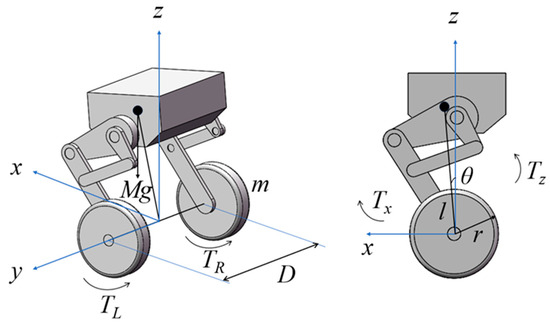
Figure 1.
Wheeled Inverted Pendulum Model and its Projection on the x-z Plane.
The Newton-Euler method is a dynamic modeling approach used to derive closed-form dynamic equations [28], which is suitable for the wheeled inverted pendulum model studied in this paper. Since the primary state variable for balance control, the tilt angle of the center of mass, is normal to the y-axis, the force analysis of the robot is conducted in the x-z plane to obtain the dynamic equations for the robot body and the main drive wheels.
where is the moment of inertia of the robot body about the y-axis, is the moment of inertia of the drive wheels about their axes, and are the driving torques of the left and right wheels, respectively, and are the additional force couples generated by the resultant forces of the drive wheels along the z-axis and x-axis, respectively, when translated to the center of mass, and are the masses of the robot body and the drive wheels, respectively, is the length of the pendulum, is the radius of the drive wheels, is the tilt angle of the center of mass.
When the robot is in a balanced posture, the tilt angle of the center of mass is small, allowing the following linearization process:
By substituting Equation (3), which neglects higher-order nonlinear terms, into Equations (1) and (2) and performing a linear expansion at the equilibrium point, the dynamic equations for the x-z plane are obtained:
When the control objective is anti-disturbance balance, four state variables are selected from the wheeled inverted pendulum model: displacement, velocity, pitch angle, and pitch angular velocity, forming the system state vector . At the same time, the driving torques of the left and right wheels are selected as the system inputs , and the system state-space model is constructed:
By substituting Equation (4) into Equation (5), the matrix expression of the state-space model is obtained:
In Equation (6), the elements , and others can be expressed as follows:
2.2. Robot’s Balanced Posture
Among the four state variables of the wheeled inverted pendulum model, the pitch angle is affected by the robot’s posture. In most application scenarios, it is desirable for the robot to maintain a horizontal body posture in the balanced state, facilitating the coordinate calculation of extensions mounted on the body [29]. Therefore, to determine the robot’s balanced posture, the following constraint is imposed on the projection of the entire system’s center of mass in the x-z plane:
where represents the x-axis coordinate of the robot’s overall center of mass, denotes the x-axis coordinates of the centers of mass for individual parts such as the upper leg and lower leg links, and represents the masses of the robot’s components. The robot maintains a balanced state when the projection of its center of mass in the x-z plane coincides with the center of the drive wheels. The robot’s posture at this time is shown in Figure 2.
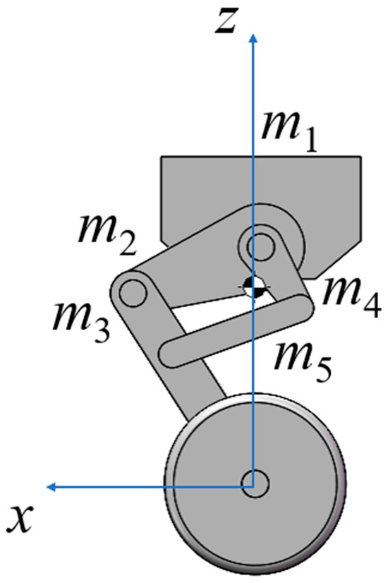
Figure 2.
Robot’s Balanced Posture.
When the robot’s height changes, the overall posture is constrained by Equation (8) to ensure the accuracy of the target state variables in the balanced state.
3. MPC Algorithm Design for WBRs
As discussed in Section 2, under wheeled motion, the WBR can be equivalently simplified to a wheeled inverted pendulum system. The wheeled inverted pendulum system is highly unstable. Without a control algorithm, the system will gradually diverge over time, making it difficult to restore balance. Therefore, a proper control algorithm is required to ensure the system’s controllability and allow it to converge over time, maintaining a balanced posture. MPC is widely used in the industrial field, and in the past decade, extensive research has been conducted on MPC’s technical selection, variable control, and performance estimation [30]. Therefore, this paper adopts MPC as the balance control algorithm for the WBR and optimizes the horizon parameters of the MPC with anti-disturbance as the control objective. The control algorithm proposed in this paper, along with the control framework applied to the robot, is shown in Figure 3.
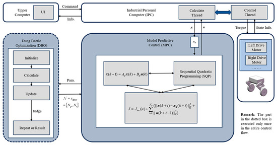
Figure 3.
Control Framework of the Robot.
In Section 3.1, the state-space equation is discretized, and a soft-constrained MPCler is formulated. Subsequently, Section 3.2 analyzes the stability of the wheeled inverted pendulum system under the MPC framework. In Section 3.3 and Section 3.4, the horizon parameters of MPC are embedded into the dung beetle optimization algorithm, and a cost function is devised to iteratively refine these parameters.
3.1. Soft-Constrained MPC Algorithm
In practical applications, the system state variables are obtained through discrete sampling during the control cycles. By discretizing Equation (5), the discrete state-space equation used for MPC calculations is obtained:
The discretization method is as follows:
where and represent the state vector and control input at time step , represents the state vector at time step , is the discretization period, and are the discretized system matrix and input matrix, respectively.
The objective of MPC is to solve an optimization problem at each sampling instant, based on the given prediction horizon and control horizon , generating a sequence of future control inputs such that the system’s behavior within the prediction horizon meets certain performance criteria. At time step , which serves as the initial sampling instant of the system, a time series is selected, yielding the system state expression with a step length of :
By rearranging Equation (11) into matrix form, it can be rewritten as:
where and are recursive matrices composed of and , respectively; is the stacked vector of future predicted states, and is the stacked vector of future control inputs, expressed as:
The following cost function is defined for MPC:
where and are the weight matrices for the state error and control input, respectively. is the desired state vector, and for anti-disturbance balance control, holds at any time step in the time series .
In the control framework of WBRs, the system’s control frequency is typically in the microsecond range to meet real-time response requirements. When the robot is subjected to disturbances, the hub motors need to respond quickly and produce large control torques. However, if the motors operate beyond their rated torque for an extended period, issues such as control lag, overheating, and reduced control precision may arise. Therefore, soft constraints need to be designed to limit the solution domain obtained through MPC, ensuring that the control inputs do not exceed the rated torque for extended periods and always remain below the peak torque.
The designed soft constraint is expressed in the form of a penalty function. Let be the constraint penalty weight and be the nonlinear acceleration factor, both of which control the magnitude of the penalty function. The value of needs to be adjusted according to the motor characteristics. From the motor characteristic curve, it is known that the heating power of the motor is proportional to the square of the current:
where is the motor current, and is the resistance of the motor windings. Let the motor’s temperature rise be denoted as :
where is the temperature rise coefficient of the motor, obtained from the motor characteristic curve. Let be the torque increment corresponding to the temperature rise . Since the current is proportional to the torque increment, the temperature rise-torque coefficient is defined as:
Based on the motor’s insulation class, the allowable temperature rise range can be selected, yielding the constraint penalty weight:
where and represent the rated torque and peak torque of the hub motor, respectively.
As for the nonlinear acceleration factor , its magnitude determines the degree of nonlinearity of the penalty function. For the hub motor of the WBR, it is necessary to provide short-term torque that exceeds the rated torque. To allow for short-term overload, the ideal range for should be between . Based on the above definitions, the following nonlinear penalty function is designed:
The reference curve of the function in Equation (19) is shown in Figure 4.
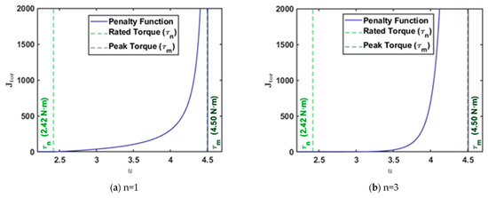
Figure 4.
Example of the Nonlinear Soft Constraint Penalty Function.
By incorporating the designed penalty function from Equation (19) into Equation (14), the final cost function of the MPC is obtained:
Using the Sequential Quadratic Programming (SQP) algorithm, Equation (20) is solved iteratively by constructing and solving a series of quadratic programming subproblems to gradually approach the optimal solution, yielding the optimal system control input for the corresponding state vector.
3.2. Stability Analysis
System stability is one of the core issues in control design, that is, whether the system can remain controllable or gradually return to the equilibrium point after being subjected to initial perturbations or external disturbances. To verify the stabilizing effect of the proposed soft-constrained MPC controller on the wheeled biped robot and its equivalent wheeled inverted pendulum system, this study conducts an eigenvalue-based stability analysis for the systems with and without the incorporation of the soft-constrained MPC controller.
In the stability analysis, an eigenvalue discrimination method based on state-space theory is adopted. This method requires only the eigenvalue calculation of the system state matrix , which enables a rapid determination of stability while avoiding complex computations. Let the eigenvalues of the continuous-time system state matrix in Equation (5) be denoted as . The following criteria apply:
- If the real parts of all eigenvalues satisfy , the system is asymptotically stable.
- If the real parts of all eigenvalues satisfy , and for those with , the corresponding Jacobian matrix has no repeated roots, the system is marginally stable.
- If there exists any eigenvalue such that , the system is unstable.
First, in the absence of the soft-constrained MPC controller, the main parameters of the robot, such as body mass and moment of inertia, are substituted into matrix , yielding the following numerical expression:
The eigenvalue calculation gives:
Since , the system is determined to be unstable. This indicates that, without control, the wheeled inverted pendulum system cannot maintain stability, and thus an appropriate controller must be introduced to ensure state convergence.
After incorporating the MPC controller, the closed-loop system matrix becomes , where is the equivalent feedback matrix given by:
Thus, the closed-loop state matrix is expressed as:
The eigenvalues of are calculated as:
The results show that all eigenvalues have negative real parts, indicating that the system achieves asymptotic stability under the soft-constrained MPC controller. Furthermore, the controllability matrix of the closed-loop system is full rank, confirming that the system remains controllable. Therefore, this analysis not only validates the effectiveness of the controller in stabilizing the wheeled inverted pendulum system but also highlights the necessity of the soft-constrained MPC in ensuring both stability and controllability.
3.3. DBO Algorithm Iteration Method
In the process of solving MPC, in addition to setting appropriate constraints, the sizes of the prediction horizon and control horizon are equally critical to computational complexity and control performance. The optimization problem in MPC essentially involves large-scale matrix computations and the iterative solution of quadratic programming problems. Proper selection of prediction and control intervals can balance computational cost and control precision. When designing the MPC algorithm for wheeled biped robots, it is necessary to determine the combination of prediction and control horizons based on the given weight matrices and . This ensures that real-time performance and anti-disturbance capability are achieved while avoiding excessive computational burden.
The Dung Beetle Optimizer (DBO) is a heuristic multi-population optimization algorithm proposed by Xue Jiankai et al. [20]. This algorithm avoids local optimal solutions through various iterative strategies and is suitable for solving multi-objective optimization problems such as in MPC. In the iterative computation process, DBO seeks the optimal solution to multi-objective optimization problems by simulating the behavior of dung beetles, generating four subpopulations: ball-rolling, breeding, foraging, and thief. Beetles in different subpopulations update their positions from the initial location according to predefined strategies. During each iteration, they calculate the cost function at their current positions based on the optimization objective, and the final position is taken as the solution to the optimization problem. The position update strategies for the four types of dung beetles are as follows:
- (1)
- Ball-Rolling Dung Beetle: Performs the most basic iterative optimization, simulating the process of beetles navigating using sunlight. Random numbers and obstacle decision number are defined to determine whether the ball-rolling dung beetle encounters an obstacle during movement. The position update equation for the obstacle-free mode is as follows:where is the current iteration count, and represents the position of the dung beetle at the iteration. is the natural coefficient, determined to be either 1 or −1 based on probabilistic distribution, representing whether the beetle deviates from its original direction. denotes the regular deflection coefficient, and denotes the sunlight deflection coefficient. is the light intensity variation, determined by the current position and the globally worst position from the previous iteration.
When the ball-rolling dung beetle encounters an obstacle, it updates its direction through a dance. The position update equation for the obstacle mode is as follows:
where determines the degree of deviation between the new direction and the original direction.
- (2)
- Breeding Dung Beetle: Uses a boundary selection strategy to simulate the dung beetle’s choice of the brooding ball region. Based on the current local optimal solution, it expands both inward and outward to generate two new solutions, thereby searching for a better solution near the local optimum. The position update equation is as follows:where is the position of the brooding ball at the iteration. and represent two independent random vectors of size . determines the extent of the brooding ball region expansion, where is the maximum number of iterations. and are the lower and upper bounds of the brooding ball region, ensuring that the region dynamically adjusts with the number of iterations. and represent the lower and upper bounds of the optimization problem, respectively. is the local optimal position at the iteration.
- (3)
- Foraging Dung Beetle: Similarly to the breeding dung beetle, it simulates the selection of a foraging area by young dung beetles. Based on the current global optimal solution, it generates two new solutions to search for a better solution near the global optimum. The position update equation is as follows:where and represent the lower and upper bounds of the foraging area, respectively. is a normally distributed random number. is a random vector following a uniform distribution. is the global optimal position at the iteration. The definitions of the remaining parameters are the same as those for the breeding dung beetle.
- (4)
- Thief Dung Beetle: It searches for a potentially better solution by mimicking the features of the current global optimal solution and introducing random perturbations. The position update equation is as follows:where is a constant that determines the magnitude of the random perturbation. represents a random vector of size following a normal distribution. The definitions of the remaining parameters are the same as those for the breeding dung beetle and the foraging dung beetle.
3.4. MPC Optimization Using the DBO Algorithm
In the optimization process of DBO, the design of the cost function affects the characteristics of the final result. For anti-disturbance scenarios, we aim for the robot to quickly return to a balanced position after being disturbed, minimizing the amplitude of body oscillation and overall displacement, while ensuring the required torque and computation time. This paper is based on the classical Integral of Time-weighted Absolute Error (ITAE) cost function, which fully accounts for the accumulated absolute values of state variables over a certain time period [31]. is defined as:
where and represent the start and duration of the experiment, respectively, and is the computation time of a single MPC calculation. , , and are the weighting parameters for the tilt angle of the center of mass, displacement, average torque, and computation time, respectively, with . The remaining parameters are defined in Equation (5).
By setting the initial values for feasible solutions and specifying the population size and number of iterations, the cost function can be iteratively optimized according to Equation (26). The main optimization process is shown in Figure 5.
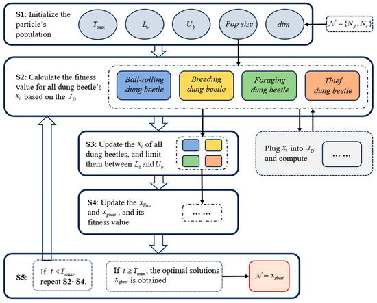
Figure 5.
The Process of DBO Optimizing N.
When calculating the position information for each dung beetle, the corresponding horizon parameter combination is transmitted into the state-space equations of the wheeled biped robot, and different types of disturbance simulations are conducted. Based on the simulation results, the cost function is calculated, updating the current optimal position and the position of each dung beetle in the next iteration. Among the four position update methods for dung beetles, the ball-rolling dung beetle serves as the basis for iterative optimization to obtain the optimal solution, with the solution given by Equations (21) and (22). Additionally, the breeding, foraging, and thief dung beetles perform extended iterative optimization around the optimal solution, with the solutions given by Equations (23)–(25), further improving the optimization efficiency.
During disturbance simulations, when is much smaller than , MPC may fail to capture key features of the system response, thereby affecting control performance. When exceeds , the insufficient prediction horizon may result in model distortion. Therefore, a larger cost function value should be assigned for these two scenarios. Moreover, during each simulation, the single computation time obtained through the tic and toc methods may vary slightly due to system frequency changes. Thus, the mean value of over the simulation should be calculated before computing the cost function. The disturbance simulation and cost function calculation process are shown in Figure 6.
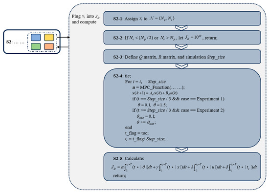
Figure 6.
DBO Disturbance Simulation and Calculation Process.
In summary, by reasonably assigning the weight parameters in , the DBO can be used to obtain an MPC algorithm that balances computational cost and control precision, enabling the WBR to achieve better anti-disturbance performance within a shorter computation time.
4. Anti-Disturbance Experiments for the WBR
This section will experimentally validate the ability of the wheeled biped robot using the MPC algorithm to restore balance under disturbance scenarios and compare it with the commonly used LQR algorithm. Additionally, it will analyze the impact of prediction horizon and control horizon on anti-disturbance performance under DBO, PSO, and non-optimized conditions.
4.1. Experimental Platform Setup
To validate the control algorithm proposed in this paper, a serial-structure wheeled bipedal robot (WBR) named SRobo110-II, independently designed and constructed by our laboratory, is used as the experimental platform [32]. The complete structure of SRobo110-II is shown in Figure 7. Its main hardware components include a TB48S battery, an N100 nine-axis Inertial Measurement Unit (IMU), HT-8115 joint motors, MF-9025 hub motors, and an Intel i5-10400H industrial computer connected externally. The IMU transmits data such as the angles and angular velocities of each axis to the industrial computer. The auxiliary wheels allow the robot to perform steering movements when powered off. Two batteries are connected in series to provide a 45.6 V power supply. The joint motors and hub motors respond to commands issued by the industrial computer, driving the links and wheels to achieve posture adjustment and movement. They also return status information such as torque and encoder positions. The serial structure of the robot is shown in Figure 8. The detailed structure and hardware parameters of the robot are listed in Table 1.
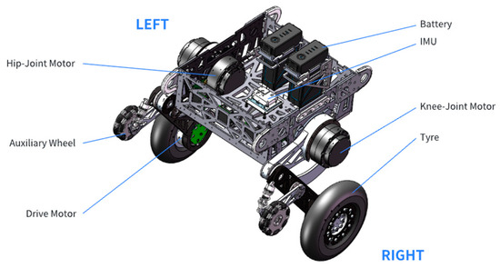
Figure 7.
Three-dimensional Model of the Complete Structure of SRobo110-II.
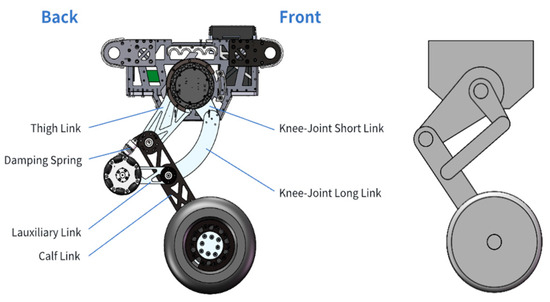
Figure 8.
Side View and Schematic of the Linkage Mechanism of SRobo110-II.

Table 1.
Structure and Hardware Parameters of SRobo110-II.
4.2. Disturbance Experiment Setup
In practical working environments, wheeled biped robots are often exposed to disturbances such as unstructured terrain, external impacts, and vertical loads. To comprehensively validate the effectiveness and superiority of the MPC horizon parameter optimization method based on DBO, as well as to evaluate the disturbance rejection capability of SRobo110-II, three types of experiments are designed in this study. First, in Experiment I, DBO is compared with PSO and ACO [33] on a simulation platform for optimizing the prediction and control horizons of MPC, and the control performance of different optimization algorithms under disturbance conditions is analyzed. Second, in Experiment II, a pendulum device is constructed using a rope and a 2 kg metal ball. The ball is pulled 1 m horizontally to the front of the robot and then released, so that it collides with the robot’s chest region—while in a balanced state—at the lowest point of its free swing. The impact velocity is determined by the pendulum length and release height, simulating sudden external forces encountered by the robot during locomotion. Finally, in Experiment III, additional mass blocks are gradually mounted onto the robot body to generate vertical load disturbances, in order to observe its posture adjustment process under load. The setups and procedures of the three experiments are illustrated in Figure 9 and Figure 10.
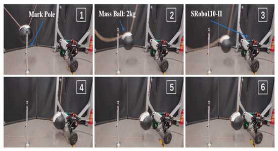
Figure 9.
Setup and Process of Expt. 1.
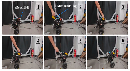
Figure 10.
Setup and Process of Expt. 2.
4.3. Expt. 1 (Simulation): Process and Result Analysis
To validate the performance of the DBO algorithm in MPC horizon parameter optimization and to systematically assess the applicability of its optimization results for disturbance rejection control of wheeled biped robots, preliminary experiments were conducted in the Webots simulation environment. As an open-source 3D robotics platform, Webots is equipped with a high-precision physics engine capable of accurately simulating essential physical effects such as gravity, friction, collision, and inertia, thus providing a reliable virtual testing environment for control algorithm verification.
The simulation experiments were carried out on a hardware platform equipped with an AMD Ryzen 7 5800H CPU (base frequency 3.20 GHz). In the Webots project, a standard floor was set as the primary interaction environment for the robot, with physical parameters carefully configured to ensure compliance with the rolling friction model assumptions between the driving wheels and the ground. Based on the wheeled biped robot platform described in Section 4.2, its simplified model was imported into Webots via the Unified Robot Description Format (URDF), with precise configuration of physical properties such as mass and inertia tensors. The structure of the imported simplified model is shown in Figure 11.
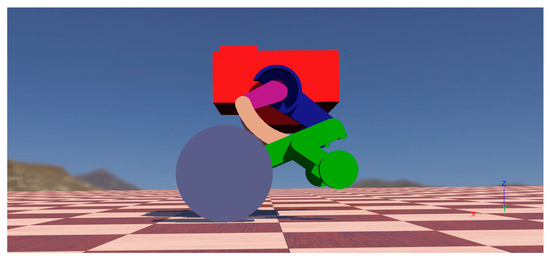
Figure 11.
Simplified model of the wheeled biped robot in Webots.
Webots also provides a comprehensive controller interface that supports co-simulation with the Visual Studio development environment. In addition to the 3D model, virtual IMU sensors, joint motors, and wheel-driving motors were configured at key positions on the robot’s body and joints. The IMU sensor continuously captured the robot’s pitch angle, which was used as a key state variable for the wheeled inverted pendulum system. Through the Visual Studio controller project, the device driver functions and state feedback functions provided by Webots enabled closed-loop interaction between robot motion control and sensor data acquisition.
To comprehensively evaluate the optimization efficiency of DBO, PSO and ACO were selected as benchmark heuristic algorithms for comparison. All three algorithms were executed under identical initial conditions, with parameter settings summarized in Table 2. To highlight the advantage of heuristic algorithms in reducing computational complexity, the maximum search count was set to 1/50 of the theoretical exhaustive count and then converted into the maximum number of iterations according to the population size. During the simulation, the step size was set to , and once the simulation time reached , the system parameter was dynamically adjusted to continuously simulate load disturbances. The final optimization results and performance comparisons are presented in Figure 12.
Table 2.
Initial condition parameters of the three heuristic algorithms.
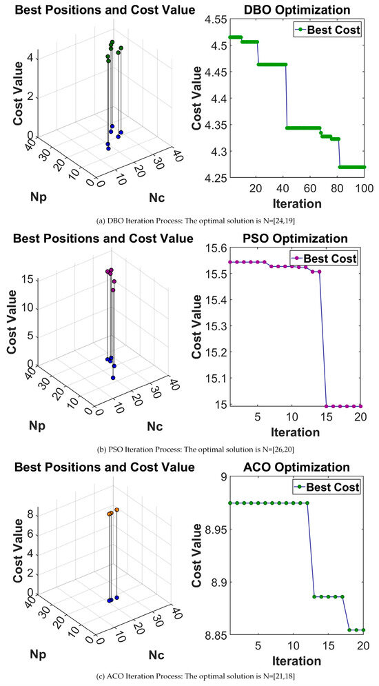
Figure 12.
Iteration under Load Disturbance and Optimal Solution Distribution.
From Figure 12, it can be seen that all three methods achieve a certain degree of iterative optimization. After 20 iterations, the optimal solution obtained by DBO yields a lower cost function value compared to PSO and ACO. The experimental results indicate that when the initial conditions are similar, the number of iterations is limited, and the computational time is comparable, DBO demonstrates superior exploration capability of the solution space. This advantage comes from its use of multiple subpopulations to perform extended iterative optimization around the optimal solution region. As a result, within a limited number of iterations, DBO exhibits better spatial search ability and is more suitable for multi-objective optimization tasks in solving MPC domain parameter combinations.
4.4. Expt. 2 (Impact): Process and Result Analysis
After completing the simulation verification in Experiment 1, further tests were conducted on the scenario where the robot is subjected to external impacts. The controller was iteratively optimized using DBO and the commonly used heuristic optimization algorithm PSO, and their control performances under impact disturbances were compared experimentally. The pseudocode of the specific implementation process is shown in Figure 6. The detailed parameter settings of the two optimization algorithms are consistent with those in Experiment 1, and the final optimization results are presented in Figure 13 and Table 3.
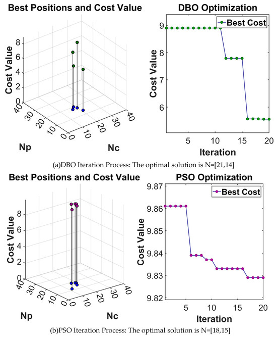
Figure 13.
Iterative Process of Impact Simulation Using DBO and PSO.
Table 3.
Parameter Combinations for Impact Experiments.
Additionally, two sets of non-optimized parameters are provided—one greater than the maximum optimized value and one smaller than the minimum optimized value—to expand the experimental control groups. The four parameter combinations from Table 3 are applied to MPC for the impact experiments. The weight matrix is configured as:
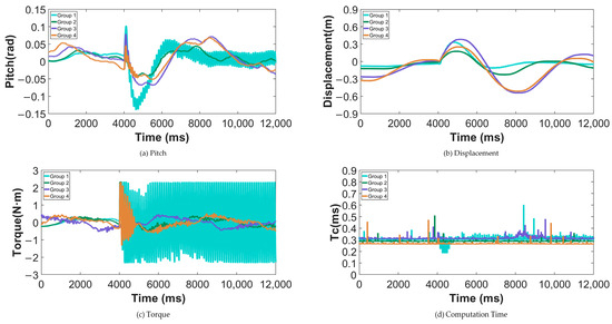
Figure 14.
Impact Experiment Results for Different Parameter Groups.
Table 4.
Impact Experiment Data for Different Parameter Groups—First Overshoot .
Table 5.
Impact Experiment Data for Different Parameter Groups—Adjustment Time .
By comparing the above experimental results, it can be seen that in all four groups of experiments, the robot was subjected to a horizontal impact from a pendulum mass at a specified moment, and data were analyzed over an 8 s interval following the disturbance. The results show that Group 1 (MPC optimized by DBO) achieved smaller first overshoots in both pitch angle and displacement compared with the other three groups, indicating a stronger capability in suppressing sudden attitude deviations and positional shifts. However, its peak torque and computation time were slightly higher. During the dynamic recovery process, Group 1 achieved the shortest adjustment time for pitch angle, while the displacement adjustment time remained at a normal level, and the torque adjustment time was slightly longer.
Further analysis suggests that this performance difference primarily stems from DBO’s multi-subpopulation cooperative search mechanism, which effectively prevents premature convergence to local optima within limited iterations and enables the discovery of superior control parameter combinations on a global scale. This allows MPC to more proactively correct disturbance errors during prediction and constraint scheduling, thereby ensuring faster convergence of pitch angle and displacement. Although this mechanism leads to an increase in peak torque and some computational overhead, both remain within a reasonable range, demonstrating that MPC optimized by DBO exhibits remarkable advantages in enhancing dynamic performance and impact disturbance rejection.
After comparing the MPC performance optimized by different heuristic algorithms, it can be observed that MPC optimized by DBO shows certain advantages in disturbance suppression. However, to further verify its superiority over traditional controllers, this study also designs an LQR-based control algorithm and conducts comparative experiments against the MPC algorithm using the Group 1 parameters. The cost function is as follows:
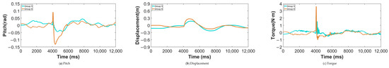
Figure 15.
Impact Experiment Results for Different Control Algorithms.
Table 6.
Impact Experiment Data for Different Control Algorithms—First Overshoot.
Table 7.
Impact Experiment Data for Different Control Algorithms—Adjustment Time.
The results of the two sets of experiments show that, after being subjected to a horizontal impact at time s, the robot controlled by MPC optimized with DBO exhibits significantly smaller overshoot in pitch angle, displacement, and torque compared with the robot controlled by LQR. Moreover, its pitch angle adjustment time is shorter, while the adjustment times for displacement and torque are slightly longer. The main reason for this difference lies in the rolling optimization mechanism of MPC, which explicitly considers future states and constraints during the control process, enabling the controller to plan ahead and suppress deviations caused by disturbances. In contrast, LQR relies on fixed feedback gains and can only provide a linear response to the current state, lacking foresight for future disturbances, which results in larger overshoot under strong perturbations. Furthermore, the DBO optimization process enables MPC to search for more suitable prediction and control horizons, as well as weight matrices, thereby achieving a better balance between rapid pitch recovery and smooth displacement adjustment, ultimately demonstrating superior disturbance rejection capability.
4.5. Expt. 3 (Load): Process and Result Analysis
Similarly to the process in Expt. 2, simulations and iterative optimizations are conducted for the robot under load disturbance using DBO and PSO. The pseudocode for the process is shown in Figure 6, and the initial values for both optimization algorithms are the same as in Expt. 1. In the cost function calculation, the simulation is also set to 1500, and is continuously adjusted at all times after to simulate load disturbance. The final optimization results are shown in Figure 16 and Table 8.
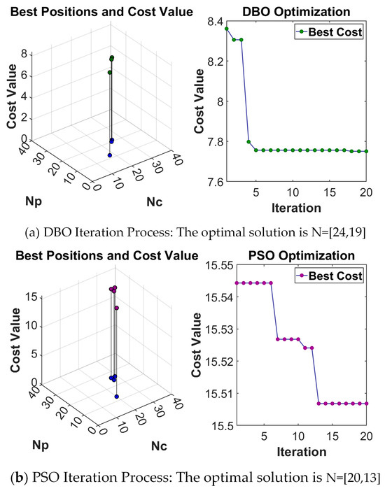
Figure 16.
Iterative Process of Load Simulation Using DBO and PSO.
Table 8.
Parameter Combinations for Load Experiments.
Similarly, two sets of non-optimized parameters are provided—one greater than the maximum optimized value and one smaller than the minimum optimized value—to expand the experimental control groups. The four parameter combinations from Table 8 are applied to the MPC algorithm for the load disturbance experiments. The weight matrix configuration is provided in Equation (23). The experimental results are shown in Figure 17 and Table 9 and Table 10.
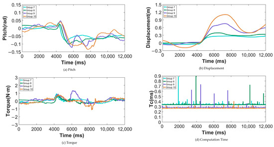
Figure 17.
Load Experiment Results for Different Parameter Groups.
Table 9.
Load Experiment Data for Different Parameter Groups—First Overshoot σ.
Table 10.
Load Experiment Data for Different Parameter Groups—Adjustment Time.
The results of the four load disturbance experiments show that MPC optimized with DBO (Group 7) outperforms the other three groups in terms of both the first overshoot and adjustment time of the pitch angle, demonstrating stronger posture recovery capability. The displacement index remains at a normal level, while the torque exhibits certain overshoot despite having a relatively better adjustment time, with computation time being slightly higher. Overall, the remarkable advantage of DBO-optimized MPC in pitch angle control stems from its subpopulation parallel search and global–local balance mechanism, which enable parameter configurations to better reconcile prediction accuracy and control stability, thereby effectively suppressing posture deviations caused by load disturbances. In contrast, the displacement and torque indicators show relatively neutral performance, reflecting that under complex coupled disturbances, the optimization mainly concentrates its performance gains on the posture dimension to ensure overall balance and safety of the robot when subjected to vertical loads.
Similarly, a comparative experiment is conducted using the designed LQR control algorithm and the MPC algorithm with the aforementioned seven-parameter configuration, with the experimental results shown in Figure 18 and Table 11 and Table 12.
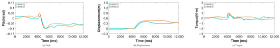
Figure 18.
Load Experiment Results for Different Control Algorithms.
Table 11.
Load Experiment Data for Different Control Algorithms—First Overshoot σ.
Table 12.
Load Experiment Data for Different Control Algorithms—Adjustment Time .
The comparison results of the two load disturbance experiments show that MPC significantly outperforms LQR in terms of overshoot of pitch angle and displacement, effectively reducing transient deviations caused by load disturbances, though its adjustment time is slightly longer; the torque adjustment time, however, performs well. This is because MPC optimizes future states in advance based on a predictive model, suppressing abrupt changes in attitude and displacement during the initial phase of the disturbance, whereas LQR, as a linear feedback control, struggles to timely compensate for transient deviations caused by nonlinear disturbances, though it has certain advantages in convergence speed. This indicates that MPC is more suitable for maintaining robot attitude stability under complex load disturbances, while LQR has relative advantages in rapid convergence.
5. Conclusions
To address the trade-off between computational cost and control precision, while enhancing the anti-disturbance capability of wheeled bipedal robots, this paper proposes a constrained Model Predictive Control (MPC) algorithm tailored to the hardware of the robot, with parameter optimization and experimental validation. The full text is summarized as follows:
- (1)
- For the wheeled motion of the wheeled bipedal robot, it is equivalently simplified to a wheeled inverted pendulum model with a variable pendulum length. A dynamic model is constructed to derive the system’s state-space model, with the balanced posture defined.
- (2)
- Based on the hardware characteristics of the robot’s drive motors, a soft-constrained MPC algorithm is proposed to prevent long-term control inputs from exceeding the rated torque, ensuring that the control input remains below the peak torque.
- (3)
- The DBO algorithm is used to appropriately select the prediction and control horizons. A cost function is defined with the goal of balancing the computational cost and control precision of the MPC, and the optimal combination for anti-disturbance is obtained through iterative optimization.
- (4)
- The SRobo-II experimental platform is constructed, and impact and load disturbance experiments are conducted on the wheeled bipedal robot. Parameters obtained through different optimization methods and control algorithms are compared and analyzed.
The experimental results show that the MPC algorithm optimized with DBO achieves smaller overshoot and faster adjustment time under both impact and load disturbances, with overall performance superior to PSO, ACO, the non-optimized version, and the LQR control algorithm. It should be noted that the MPC algorithm designed and optimized in this work is still based on a simplified equivalent first-order wheeled inverted pendulum model. When the robot’s height or posture changes significantly, the model needs to be reconstructed or adjusted. Therefore, future research will focus on further refining the dynamic model, fully accounting for the influence of structural variations such as the torso, and exploring hierarchical control architectures to achieve stable and disturbance-resistant control under varying pose conditions.
Author Contributions
Conceptualization, W.C. and Y.F.; methodology, W.C.; software, W.C.; validation, W.C., Y.F. and T.Z.; formal analysis, W.C.; investigation, W.C.; resources, C.P.; data curation, W.C.; writing—original draft preparation, Y.F.; writing—review and editing, W.C. and C.P.; visualization, W.C.; supervision, T.Z.; project administration, T.Z.; funding acquisition, W.C. All authors have read and agreed to the published version of the manuscript.
Funding
This research was funded by the Natural Science Foundation of Guangdong Province (Project No. 2024A1515012637) and the Key Research and Development Project of Guangdong Province (Project No. 2021B0101420003), China. The APC was funded by Doctoral Fund of Guangzhou City University of Technology (Grant No. KY200102).
Data Availability Statement
The raw data supporting the conclusions of this article will be made available by the authors on request.
Acknowledgments
The authors would like to thank the Robotics Laboratory of South China University of Technology for providing the experimental facilities. During the preparation of this manuscript, the authors used language editing tools for polishing and MATLAB R2024b for data analysis. All generated content has been carefully reviewed and edited by the authors, who take full responsibility for the final version of the manuscript.
Conflicts of Interest
The authors declare no conflicts of interest. The funders had no role in the design of the study; in the collection, analyses, or interpretation of data; in the writing of the manuscript; or in the decision to publish the results.
References
- Boston Dynamics. Legacy Robot: Handle. 2019. Available online: http://www.bostondynamics.com/legacy (accessed on 1 May 2024).
- Mao, N.; Chen, J.; Spyrakos-Papastavridis, E.; Dai, J.S. Dynamic modeling of wheeled biped robot and controller design for reducing chassis tilt angle. Robotica 2024, 42, 2713–2741. [Google Scholar] [CrossRef]
- Xin, Y.; Li, Y.; Chai, H.; Rong, X.; Ruan, J. Planning and Execution of Dynamic Whole-body Locomotion for a Wheeled Biped Robot on Uneven Terrain. Int. J. Control. Autom. Syst. 2024, 22, 1337–1348. [Google Scholar] [CrossRef]
- Sikander, A.; Prasad, R. Reduced order modelling based control of two wheeled mobile robot. J. Intell. Manuf. 2017, 30, 1057–1067. [Google Scholar] [CrossRef]
- Karthika, B.; Jisha, V.R. Nonlinear Optimal Control of a Two Wheeled Self Balancing Robot. In Proceedings of the 2020 5th IEEE International Conference on Recent Advances and Innovations in Engineering (ICRAIE), Jaipur, India, 1–3 December 2020; pp. 1–6. [Google Scholar]
- Cui, L.; Wang, S.; Zhang, J.; Zhang, D.; Lai, J.; Zheng, Y.; Zhang, Z.; Jiang, Z.P. Learning-Based Balance Control of Wheel-Legged Robots. IEEE Robot. Autom. Lett. 2021, 6, 7667–7674. [Google Scholar] [CrossRef]
- Dong, J.Y.; Liu, R.; Lu, B.; Guo, X.; Liu, H.W. LQR-based Balance Control of Two-wheeled Legged Robot. In Proceedings of the 41st Chinese Control Conference (CCC), Hefei, China, 25–27 July 2022; pp. 450–455. [Google Scholar]
- Katayama, S.; Murooka, M.; Tazaki, Y. Model predictive control of legged and humanoid robots: Models and algorithms. Adv. Robot. 2023, 37, 298–315. [Google Scholar] [CrossRef]
- Cychowski, M.; Szabat, K.; Orlowska-Kowalska, T. Constrained Model Predictive Control of the Drive System with Mechanical Elasticity. IEEE Trans. Ind. Electron. 2009, 56, 1963–1973. [Google Scholar] [CrossRef]
- Mishra, A.; Bansal, K. Control of Two-Wheel Self-Balancing Robot: LQR and MPC Performance Analysis. In Proceedings of the 2024 IEEE International Students’ Conference on Electrical, Electronics and Computer Science (SCEECS), Bhopal, India, 24–25 February 2024; pp. 1–6. [Google Scholar]
- Khatoon, S.; Chaturvedi, D.K.; Hasan, N.; Istiyaque, M. Optimal Controller Design for Two Wheel Mobile Robot. In Proceedings of the 2018 3rd International Innovative Applications of Computational Intelligence on Power, Energy and Controls with their Impact on Humanity (CIPECH), Ghaziabad, India, 1–2 November 2018; p. 5. [Google Scholar]
- Yu, J.; Zhu, Z.; Lu, J.; Yin, S.; Zhang, Y. Modeling and MPC-Based Pose Tracking for Wheeled Bipedal Robot. IEEE Robot. Autom. Lett. 2023, 8, 7881–7888. [Google Scholar] [CrossRef]
- Minouchehr, N.; Hosseini-Sani, S.K. Design of Model Predictive Control of Two-Wheeled Inverted Pendulum Robot. In Proceedings of the 3rd RSI/ISM International Conference on Robotics and Mechatronics (ICROM), Tarbiat Modares Univ, Tehran, Iran, 7–9 October 2015; pp. 456–462. [Google Scholar]
- Kanneworff, M.; Belvedere, T.; Scianca, N.; Smaldone, F.M.; Lanari, L.; Oriolo, G. Task-Oriented Generation of Stable Motions for Wheeled Inverted Pendulum Robots. In Proceedings of the 2022 International Conference on Robotics and Automation (ICRA), Philadelphia, PA, USA, 23–27 May 2022; pp. 214–220. [Google Scholar]
- Cao, H.X.; Lu, B.; Liu, H.W.; Liu, R.; Guo, X. Modeling and MPC-based balance control for a wheeled bipedal robot. In Proceedings of the 41st Chinese Control Conference (CCC), Hefei, China, 25–27 July 2022; pp. 420–425. [Google Scholar]
- Fernandez, D.C.; Hollinger, G.A. Model Predictive Control for Underwater Robots in Ocean Waves. IEEE Robot. Autom. Lett. 2017, 2, 88–95. [Google Scholar] [CrossRef]
- Li, X.; Gu, J.; Huang, Z.; Wang, W.; Li, J. Optimal design of model predictive controller based on transient search optimization applied to robotic manipulators. Math. Biosci. Eng. 2022, 19, 9371–9387. [Google Scholar] [CrossRef]
- Kashyap, A.K.; Parhi, D.R. Optimization of stability of humanoid robot NAO using ant colony optimization tuned MPC controller for uneven path. Soft Comput. 2021, 25, 5131–5150. [Google Scholar] [CrossRef]
- Chen, Z.; Lai, J.; Li, P.; Awad, O.I.; Zhu, Y. Prediction Horizon-Varying Model Predictive Control (MPC) for Autonomous Vehicle Control. Electronics 2024, 13, 1442. [Google Scholar] [CrossRef]
- Jin, M.; Li, J.; Chen, T. Method for the Trajectory Tracking Control of Unmanned Ground Vehicles Based on Chaotic Particle Swarm Optimization and Model Predictive Control. Symmetry 2024, 16, 708. [Google Scholar] [CrossRef]
- Qazani, M.R.C.; Tabarsinezhad, F.; Asadi, H.; Khanam, S.; Arogbonlo, A.; Nahavandi, D.; Mohamed, S.; Lim, C.P.; Nahavandi, S. Optimal MPC Horizons Tunning of Nonlinear MPC for Autonomous Vehicles Using Particle Swarm Optimisation. In Proceedings of the 2022 IEEE International Conference on Systems, Man, and Cybernetics (SMC), Prague, Czech Republic, 9–12 October 2022; pp. 635–641. [Google Scholar]
- Xue, J.; Shen, B. Dung beetle optimizer: A new meta-heuristic algorithm for global optimization. J. Supercomput. 2022, 79, 7305–7336. [Google Scholar] [CrossRef]
- Yang, P.; Sun, L.; Zhang, M.; Chen, H. A lightweight optimal design method for magnetic adhesion module of wall-climbing robot based on surrogate model and DBO algorithm. J. Mech. Sci. Technol. 2024, 38, 2041–2053. [Google Scholar] [CrossRef]
- Li, Y.; Sun, K.; Yao, Q.; Wang, L. A dual-optimization wind speed forecasting model based on deep learning and improved dung beetle optimization algorithm. Energy 2024, 286, 129604. [Google Scholar] [CrossRef]
- Cao, W.; Liu, Z.; Song, H.; Li, G.; Quan, B. Dung Beetle Optimized Fuzzy PID Algorithm Applied in Four-Bar Target Temperature Control System. Appl. Sci. 2024, 14, 4168. [Google Scholar] [CrossRef]
- Liu, F.; Luo, J.; Mo, J.; Gao, C.; Song, Z. Modeling and analysis of rigid-flexible coupling dynamics of a cable-driven manipulator. J. Mech. Sci. Technol. 2024, 38, 4377–4384. [Google Scholar] [CrossRef]
- Zhao, H.; Yu, L.; Qin, S.; Jin, G.; Chen, Y. Design and Control of a Bio-Inspired Wheeled Bipeda Robot. IEEE/ASME Trans. Mechatron. 2025, 30, 2461–2472. [Google Scholar] [CrossRef]
- Driels, M.R.; Fan, U.J.; Pathre, U.S. The application of newton-euler recursive methods to the derivation of closed form dynamic equations. J. Robot. Syst. 2007, 5, 229–248. [Google Scholar] [CrossRef]
- Liu, T.; Zhang, C.; Wang, J.; Song, S.; Meng, M.Q.H. Towards Terrain Adaptablity: In Situ Transformation of Wheel-Biped Robots. IEEE Robot. Autom. Lett. 2022, 7, 3819–3826. [Google Scholar] [CrossRef]
- Qin, S.J.; Badgwell, T.A. A survey of industrial model predictive control technology. Control. Eng. Pract. 2003, 11, 733–764. [Google Scholar] [CrossRef]
- Mudi, R.K.; Pal, N.R. A robust self-tuning scheme for PI- and PD-type fuzzy controllers. IEEE Trans. Fuzzy Syst. 1999, 7, 2–16. [Google Scholar] [CrossRef]
- Zhang, A.; Zhou, R.; Zhang, T.; Zheng, J.; Chen, S. Balance Control Method for Bipedal Wheel-Legged Robots Based on Friction Feedforward Linear Quadratic Regulator. Sensors 2025, 25, 1056. [Google Scholar] [CrossRef] [PubMed]
- Dorigo, M.; Gambardella, L.M. Ant Colony System: A Cooperative Learning Approach to the Traveling Salesman Problem. IEEE Trans. Evol. Computat. 1997, 1, 53–66. [Google Scholar] [CrossRef]


Disclaimer/Publisher’s Note: The statements, opinions and data contained in all publications are solely those of the individual author(s) and contributor(s) and not of MDPI and/or the editor(s). MDPI and/or the editor(s) disclaim responsibility for any injury to people or property resulting from any ideas, methods, instructions or products referred to in the content. |
© 2025 by the authors. Licensee MDPI, Basel, Switzerland. This article is an open access article distributed under the terms and conditions of the Creative Commons Attribution (CC BY) license (https://creativecommons.org/licenses/by/4.0/).