Article

A Novel Empirical-Informed Neural Network Method for Vehicle Tire Noise Prediction

School of Mechanical Engineering, Southwest Jiaotong University, Chengdu 610031, China
*
Author to whom correspondence should be addressed.
Machines 2025, 13(10), 911; https://doi.org/10.3390/machines13100911
Submission received: 3 September 2025 / Revised: 20 September 2025 / Accepted: 24 September 2025 / Published: 2 October 2025
(This article belongs to the Section Vehicle Engineering)

Abstract

In the evaluation of vehicle noise, vibration and harshness (NVH) performance, interior noise control is the core consideration. In the early stage of automobile research and development, accurate prediction of interior noise caused by road surface is very important for optimizing NVH performance and shortening the development cycle. Although the data-driven machine learning method has been widely used in automobile noise research due to its advantages of no need for accurate physical modeling, data learning and generalization ability, it still faces the challenge of insufficient accuracy in capturing key local features, such as peaks, in practical NVH engineering. Aiming at this challenge, this paper introduces a forecast approach that utilizes an empirical-informed neural network, which aims to integrate a physical mechanism and a data-driven method. By deeply analyzing the transmission path of interior noise, this method embeds the acoustic mechanism features such as local peak and noise correlation into the deep neural network as physical constraints; therefore, this approach significantly enhances the model’s predictive performance. Experimental findings indicate that, in contrast to conventional deep learning techniques, this method is able to develop better generalization capabilities with limited samples, while still maintaining prediction accuracy. In the verification of specific models, this method shows obvious advantages in prediction accuracy and computational efficiency, which verifies its application value in practical engineering. The main contributions of this study are the proposal of an empirical-informed neural network that embeds vibro-acoustic mechanisms into the loss function and the introduction of an adaptive weight strategy to enhance model robustness.

1. Introduction

Due to the fast-paced advancements in science and technology and the continuous improvement of residents’ living standards, people’s need for automobiles is no longer limited to the function of transportation but gives more attention to the comfort experience in the process of driving. The noise, vibration and harshness (NVH) performance of vehicles has an important impact on the psychological and physical health of drivers and passengers. In the context of the increasing popularity of electric vehicles, the powertrain noise is significantly reduced, and the road structure noise has gradually become an important part of the cabin noise of the vehicle. Its proportion and influence are increasing, which exerts a considerable influence on the vehicle’s overall sound performance [1,2,3]. Under urban road conditions, tire noise often constitutes the primary origin of noise within the vehicle and significantly exceeds power system and aerodynamic noise. The main excitation of road structural noise comes from road roughness [4]. As the vehicle speed increases, the excitation effect of road surface increases, which is transmitted to the vehicle’s body via the suspension and body mounting components, causing the vibration of the body plate. When the structural vibration mode is coupled with the acoustic mode, it is prone to over-response, forming a high-amplitude low-frequency sound pressure fluctuation in the vehicle, resulting in a low-frequency roar perceived by the occupants [5]. This kind of noise not only significantly lowers the vehicle’s acoustic comfort, but also may cause passengers to experience chest tightness, dizziness, nausea and other discomfort. Thus, controlling road structure noise plays a crucial role in optimizing and designing the vehicle’s NVH performance.
As computer technology and acoustic theory continue to advance, the research on vehicle tire noise has gradually expanded from early dependence on a single test to simulation analysis based on computer-aided engineering (CAE), and then to the current comprehensive research mode combining test and CAE. This method has become a conventional technical path in the research and development of major automobile enterprises, and a variety of improvement methods have emerged in this process. Contartese et al. [6] introduced an innovative approach to impose two physical properties on the experimental frequency response function model, recognizing that the inaccuracy of subsystems derived from experiments often significantly impacts the prediction of the combined system’s behavior. Yuan and Yang et al. [7] proposed a new method to detect the transverse cracking of pavement by using the reconstructed vehicle vibration signal, and effectively analyzed the related performance of pavement. The results indicate that the designed magnetic suspension system offers outstanding vibration isolation performance, with power loss being less than 1/1000 of the vehicle engine’s power, thus providing a novel approach for tire noise control. Huang and Mikhailenko et al. [8,9] reviewed the Close-Proximity, Statistical Pass-By and On-Board Sound Intensity methods, and found that optimizing surface texture on a macro scale is important for reducing tire/tire noise. Porous asphalt concrete pavements and their variants are among the most effective in achieving low noise performance. From the existing research progress, scholars have carried out extensive exploration around the traditional tire noise analysis method and put forward improvement measures from different angles, having achieved positive results in engineering applications. However, this type of method usually has a long test cycle and high cost and involves complex mechanism modeling, which leads to its computational efficiency remaining insufficient.
The data analysis method driven by machine learning can effectively describe the mapping relationship between complex variables with its surrogate model. It has been gradually introduced into the field of vehicle NVH research to improve the efficiency of analysis and prediction. Deubel et al. [10] proposed a test data training artificial neural network model based on high-quality subjective ratings, which can accurately predict the virtual subjective perception rating corresponding to the specific load conditions of the human body. Dai et al. [11] proposed a random forest algorithm based on particle swarm optimization. The subjective and objective data obtained from the experiment were used to train the prediction model, the objective input dimension was reduced by correlation analysis, and the accurate prediction of the sound quality of construction machinery was realized. Huang et al. [12] proposed a research method for prediction and optimization of tire / road structural noise of pure electric vehicles by combining knowledge graph and multi-task technology. This method not only improves the efficiency of computation but also improves the prediction accuracy of the model. Although the data-driven method has shown good results in some NVH applications, the efficient prediction of vehicle interior noise still faces challenges. On the one hand, the neural network model relies heavily on training samples, especially in the case of complex network scale, which necessitates substantial labeled data support. When the training samples are insufficient, the model tends to overfit, which leads to prediction failure [13]. On the other hand, in some engineering practices, the evaluation and decision-making results of the data-driven method output lack clear interpretability, which makes it difficult for design engineers to accept the opaque model of its internal mechanism, thus limiting its engineering application [14].
While machine learning-based data-driven methods face various challenges in predicting internal vehicle noise, a novel machine learning approach, Physics-Informed Neural Networks (PINNs), provides new ideas for solving these problems. It was originally proposed by Raissi et al. [15]. It has garnered significant attention due to its ability to be trained for supervised learning tasks and its compatibility with any given physical law described by general nonlinear partial differential equations. This method offers notable advantages in solving both forward and backward partial differential equation (PDE) problems, such as applications in Navier–Stokes equations [16], stochastic PDEs [17] and fractional PDEs [18]. In addition, PINNs have achieved remarkable results in a range of problems in mechanical engineering and related fields, including fault diagnosis [19,20], metamaterials [21], etc. Cai et al. [22] applied PINNs to the solution of heat transfer problems and achieved good results, demonstrating its potential in electronic power-related industrial applications. Li and Zhang [23] incorporated the physical characteristics of the wind turbine system into a data-driven model, utilizing the system’s structural features and linearized representation as physical constraints. These were then applied to a deep residual recurrent neural network, resulting in a deep learning model that integrates physical information. Numerical simulations show the accuracy and efficiency of the method. The PINNs’ loss function is formulated as a fixed weighted sum of observed data, boundary conditions and initial constraints, and PDE residuals [24,25,26]. This combination strategy offers a robust tool for the modeling and prediction of complex systems. Especially in the case of sparse or incomplete data, it can use fewer data samples to learn models with stronger generalization ability [27,28,29,30]. However, its training efficiency is highly dependent on the weight associated with different loss items. By manually adjusting these weights to balance the relative importance of each loss item, not only is it time-intensive and laborious, but it is also susceptible to errors and omissions [31,32]. In addition, due to the complexity of the vehicle suspension system, it is difficult to establish an accurate local differential equation model, which makes it difficult for the PINNs method to be directly applied to tire noise prediction.
This paper makes its primary contributions in two key areas:
(1)
This study proposes an Empirical-informed Neural Network (EINN) method. By redesigning the neural network’s loss function, the local vibro-acoustic mechanism is embedded in it in the form of constraints. Even in the absence of an accurate physical model, this method can use empirical data to guide network learning and construct a hybrid neural network model that combines knowledge and data-driven methods. This innovation successfully addresses the traditional physical information neural network’s reliance on precise physical models when handling complex systems, thereby greatly broadening its scope of application.
(2)
To enhance the model’s prediction performance further, this study introduces an adaptive weight mechanism. The mechanism can dynamically adjust the weight of each item in the loss function to ensure the numerical comparability of different weights, so as to effectively prevent gradient disappearance or gradient explosion and significantly improve the robustness of the training process.
This paper is organized as follows: The second section first introduces the traditional convolutional neural network (CNN) method, and on this basis, an improved empirical-informed neural network model is proposed. The third section describes the experimental design in detail and analyzes the experimental results in depth. The fourth section implements the prediction method proposed in this paper and verifies the results. The fifth section summarizes the full text. Figure 1 illustrates the technical approach of the proposed method.

2. Method Proposed

2.1. Introduction of CNN Structure

A Convolutional Neural Network (CNN) is a deep learning model well-suited for grid-structured data such as images, speech, and time-series signals [33,34,35]. Compared with fully connected networks, CNNs significantly reduce parameters through local receptive fields, weight sharing and pooling, while maintaining strong feature extraction capability. In vehicle acoustic and vibration analysis, where signals exhibit rich time–frequency features, CNNs can suppress redundancy and retain key local modes, making them widely applied in NVH prediction. In addition, CNNs are particularly effective at extracting hierarchical features from matrix inputs, whereas models such as long short-term memory networks or gated recurrent units are more suitable for purely sequential data.
Figure 2 illustrates a typical CNN architecture, which is composed of an input layer, convolutional layers, nonlinear activation layers, pooling layers, and fully connected layers [36,37]. The input layer accepts external signals in the form of vectors or matrices. Convolutional layers apply convolution kernels to local regions to extract hierarchical features, while activation layers introduce nonlinearity to enhance the network’s ability to model complex relationships. Pooling layers reduce feature dimensions and improve robustness against translation and small perturbations. Finally, fully connected layers integrate the extracted features and map them to the output space to complete prediction tasks. This hierarchical structure enables CNNs to progressively transform low-level input data into high-level abstract representations, which is particularly useful for acoustic and vibration signal modeling [38].
In the convolution layer, the core operation is the convolution operation of the input data and the convolution kernel. Let the input feature map be X R H × W and the convolution kernel be K R m × n , then the convolution operation is expressed as follows:
Y ( i , j ) = p = 1 m q = 1 n K ( p , q ) X ( i + p 1 , j + q 1 ) + b
where Y i , j corresponds to the convolution output at the position i , j , K p , q   is the weight of the convolution filter applied to the input window dimensions, and b stands for the bias term.
When the convolution outputs are processed by a nonlinear activation function, they can effectively expand the network’s expressive power, enabling it to model more complex relationships. Activation functions that are frequently employed in neural networks include the Sigmoid function, the hyperbolic tangent (tanh), and the Rectified Linear Unit (ReLU). Among them, the ReLU function is widely used in deep CNNs because of its simple calculation and ability to alleviate the problem of gradient disappearance. The function remains linear when the input is greater than zero, otherwise the output is zero; the ReLU function is defined as follows:
f ( x ) = max ( 0 , x )
In the feature extraction process, the pooling layer is often used for downsampling to reduce the spatial dimension of the feature map and reduce the computational complexity. Pooling operations are mainly divided into Max Pooling and Average Pooling. Taking the maximum pooling as an example, if the size of the pooling window is r   ×   r, the operation selects the maximum value as the output in each window, then the pooling output can be expressed as follows:
Y ( i , j ) = max ( p , q ) r × r X ( i + p 1 , j + q 1 )
After multi-layer convolution and pooling, CNN can gradually combine low-level local features into high-level abstract representations. In the final fully connected layer, these abstract features are expanded and mapped to the output space. Suppose the input vector of the fully connected layer is x, the weight matrix is W, and the bias is b, then the output can be represented by a linear transformation (regression problem):
y = W   x + b
If the task is a classification problem, it is usually necessary to introduce a Softmax function in the output layer to convert the prediction result into a probability distribution. The equation is as follows:
P ( y i ) = e z i j = 1 k e z j ,   i = 1 , 2 , , k
where z i represents the i-th element of the output vector generated by the fully connected layer, and P y i denotes the probability of belonging to category i.
In practical engineering, the network depth and the number of convolution kernels of CNN can be flexibly set according to task complexity and data size. With the help of local connection, weight sharing and the pooling mechanism, CNN can significantly reduce the number of parameters and improve the generalization performance of the model while maintaining the expression ability. In contrast to a fully connected network, CNN can extract stable features more efficiently in multi-dimensional nonlinear problems, so it has significant application potential in tasks such as vehicle acoustic packet optimization and noise prediction.

2.2. EINN Proposed

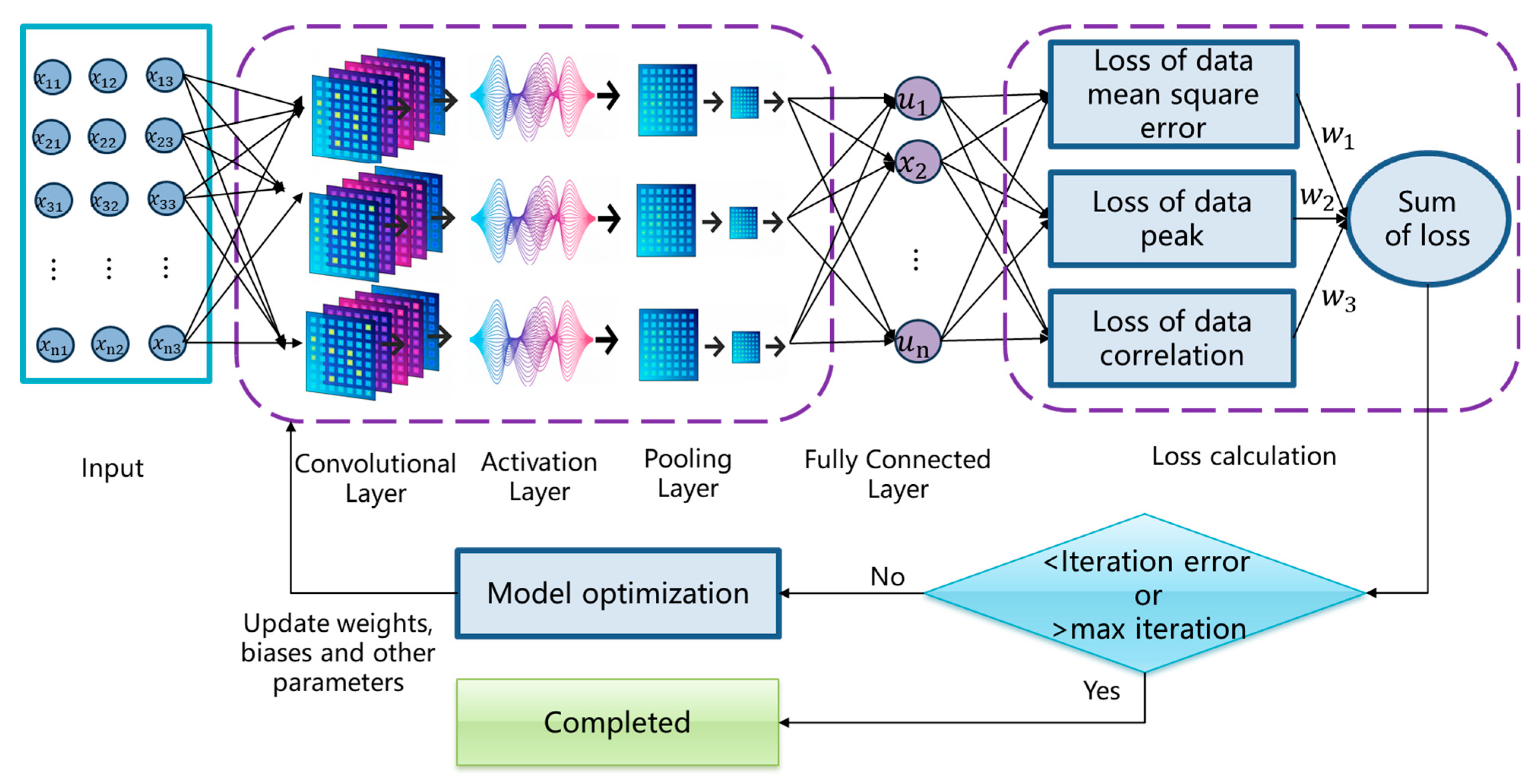
Based on the concept of a PINN, this paper further refines and extends the loss function to better incorporate domain knowledge. On the CNN backbone, the value calculated from the empirical formula is introduced into the network as an additional constraint, guiding the model to satisfy physical relationships and enhancing its suitability for road noise prediction. The proposed EINN integrates both data-driven learning and empirical knowledge, forming a hybrid architecture. As illustrated in Figure 3, the network consists of the following: an input layer receiving vehicle and road feature vectors; multiple convolutional and activation layers for hierarchical feature extraction; a constraint module where empirical model outputs are incorporated; and fully connected layers that map the combined features to the predicted noise spectrum. This structure allows the EINN to leverage both measured data and prior empirical knowledge, improving predictive accuracy and generalization for road-induced interior noise.
The loss function of the EINN is composed of three distinct parts. The first part corresponds to the loss term from traditional data-driven models, which primarily focuses on quantifying the difference between the predicted values and the actual observed values, as shown in Equation (6):
l o s s d = 1 N d i = 1 N d u p r e u r e a l 2
Here, u p r e is the output value of the neural network, u r e a l is the label value, and N p is the feature dimension. The role of this loss term is to maintain the closeness of the model’s output to the complete training set, thus providing a standard for the model to meet during the learning process.
The second part is the peak error loss term of the predicted sequence features, as shown in Equation (7):
l o s s p = 1 N p i = 1 N p u p r e peak u r e a l peak 2
This shows the peak value of the predicted output of the u p r e p e a k neural network in a certain frequency range; u p r e p e a k is the peak of the label value in a certain frequency range, and N p is the number of data points near the characteristic peak. This loss term calculates the mean square error between the neural network output and the true value near the peak position. The purpose is to ensure that the neural network output is closely matched with the true value at the characteristic peak, which is crucial for maintaining the model’s performance.
To compute the third loss, the correlation loss, we first calculate the Pearson correlation coefficient between the variables, and then take the reciprocal of the loss function associated with it, providing a measure of the relationship between them, as shown in Equation (8):
l o s s c = 1 / i = 1 N c ( u p r e d u ¯ p r e d ) ( u r e a l u ¯ r e a l ) i = 1 N c ( u p r e d u ¯ p r e d ) 2 i = 1 N c ( u r e a l u ¯ r e a l ) 2
Among them, N r is the number of data points, u ¯ p r e d is the average value of the network output characteristics, and u ¯ r e d is the average value of the label value. This loss term is used to measure the correlation between the predicted neural network’s output and the actual value’s label value. By calculating the Pearson correlation coefficient of the network output sequence u p r e and the label value sequence u r e a l , the linear relationship strength between them can be obtained. The loss function is the reciprocal of the correlation coefficient. When the output is completely related to the label, the loss is smaller. When the output is not related to the label, the loss is larger, which can effectively guide the network training. The overall loss of the network is represented in Equation (9):
l o s s E I N N s = ω d l o s s d + ω p l o s s p + ω c l o s s c
Among them, ω d is the loss weight in the traditional neural network model, ω p is the local loss weight of the feature peak, and ω c is the loss weight of the sequence correlation error. Just as in typical machine learning models, the loss function weights are fixed, and the training effectiveness depends on how the weights are assigned to various loss components. Nevertheless, the conventional approach to modifying the loss weights is labor-intensive, time-consuming, and susceptible to mistakes and oversights. Based on this, this paper proposes an adaptive weight algorithm based on a normalized adaptive method, which normalizes each weight item so that they contribute equal weight to the total loss, ensuring that no single loss item is biased during model training. This method helps to improve the generalization ability of the model and usually accelerates the convergence speed of the model because it avoids the training instability caused by the overemphasis of a single loss term.
Specifically, before the training starts, the average value of each loss item is calculated by forward propagation. Using the calculated average loss value, the initial normalized weight is set. These weights are applied to adjust the impact of each loss component on the overall loss. Each normalized adaptive weight update is shown in Equation (10):
ω d = 1 / σ d N d ω p = 1 / p N p ω c = 1 / σ c N c
Among them, σ d , σ p and σ c represent the standard deviation of the data loss term, the peak error loss term and the correlation error loss term in the initial training stage, respectively. N d , N p and N c represent the sample size in the data loss term, the peak error loss term and the correlation error loss term, respectively. Then, in each forward propagation, the normalized adaptive weight is used to calculate the total loss as shown in Equation (11):
L o s s E I N N s = ω d M S E d + ω p M S E p + ω c M S E c
In each iteration, these normalized adaptive weights are dynamically updated to reflect the relative importance of different loss items in the model training process. Such a dynamic normalization adaptive process can not only guarantee that the model rapidly adjusts to data and physical laws during the early stages of learning but also automatically adjust in the later training to avoid overfitting any loss term.
Compared with other recent hybrid ML models in NVH studies, such as LSTM and GRU networks that emphasize temporal sequence learning or ResNet variants that enhance feature extraction through residual connections, the proposed EINN differs by explicitly embedding empirical physical knowledge into the network architecture and loss function. This integration allows EINN not only to learn data-driven representations but also to adhere to underlying physical constraints, thereby improving interpretability and robustness in road noise prediction.

3. Vehicle Tire Noise Test and Analysis

3.1. Analysis of Factors Affecting Tire Noise

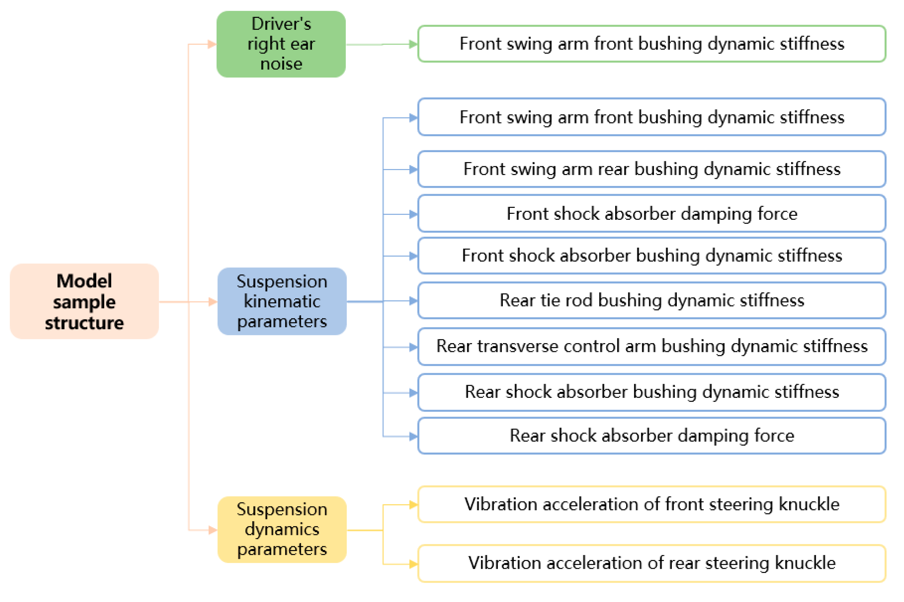
During the assessment of vehicle structural vibration and noise, each system can be described by the ‘source-path-receiver’ model, and the suspension system also follows this model [39]. In an actual driving scene, the excitation generated by the contact between the tire and the road surface is transmitted to the body through the suspension system, causing structural vibration and generating radiated noise, which is finally perceived by the human ear. This transmission mechanism reveals the key factors of structural sound in tire noise, including road excitation, tire characteristics and the properties of elastic connecting elements in suspension system. In engineering practice, because the tire stiffness and damping parameters are difficult to obtain accurately and the adjustment is limited, the steering knuckle vibration excitation is usually used as the load input of the model. This processing method effectively avoids the complexity of directly studying the interaction between tire and road surface, thus simplifying the construction of the tire noise prediction model. In the analysis of an automobile suspension system, the stiffness of the helical spring has a relatively small influence on the system frequency, and the direct influence on the tire noise is limited [40]. In contrast, the bushing and shock absorber in the suspension system, as the main vibration isolation components, have a more significant impact on tire noise. Therefore, this study highlights the dynamic stiffness of the bushing and the damping characteristics of the shock absorber as crucial dynamic parameters [41]. The experiment focuses on a vehicle equipped with a ‘front McPherson and rear multi-link’ suspension system, and its structural parameters are analyzed in detail, as illustrated in Figure 4.

3.2. Tire Noise Road Test

In order to obtain the vibration data of the steering knuckle, suspension and body connection points, as well as the noise data of the driver‘s right ear, this study carried out a real vehicle road test and simultaneously collected the noise and vibration data of the test vehicle under different road conditions. The 24-channel LMS SCADAS data acquisition system and LMS Testlab 2021.1 software produced by LMS Company of Belgium were used in the experiment, which were used for online data acquisition, analysis and processing. The noise signals were captured using a non-directional BSWA sound pressure sensor, while vibration signals were recorded with a PCB three-axis vibration sensor [42]. The sampling duration was set to 10 s, with a sampling frequency of 6400 Hz for both noise and vibration signals, yielding a frequency resolution of 1 Hz.
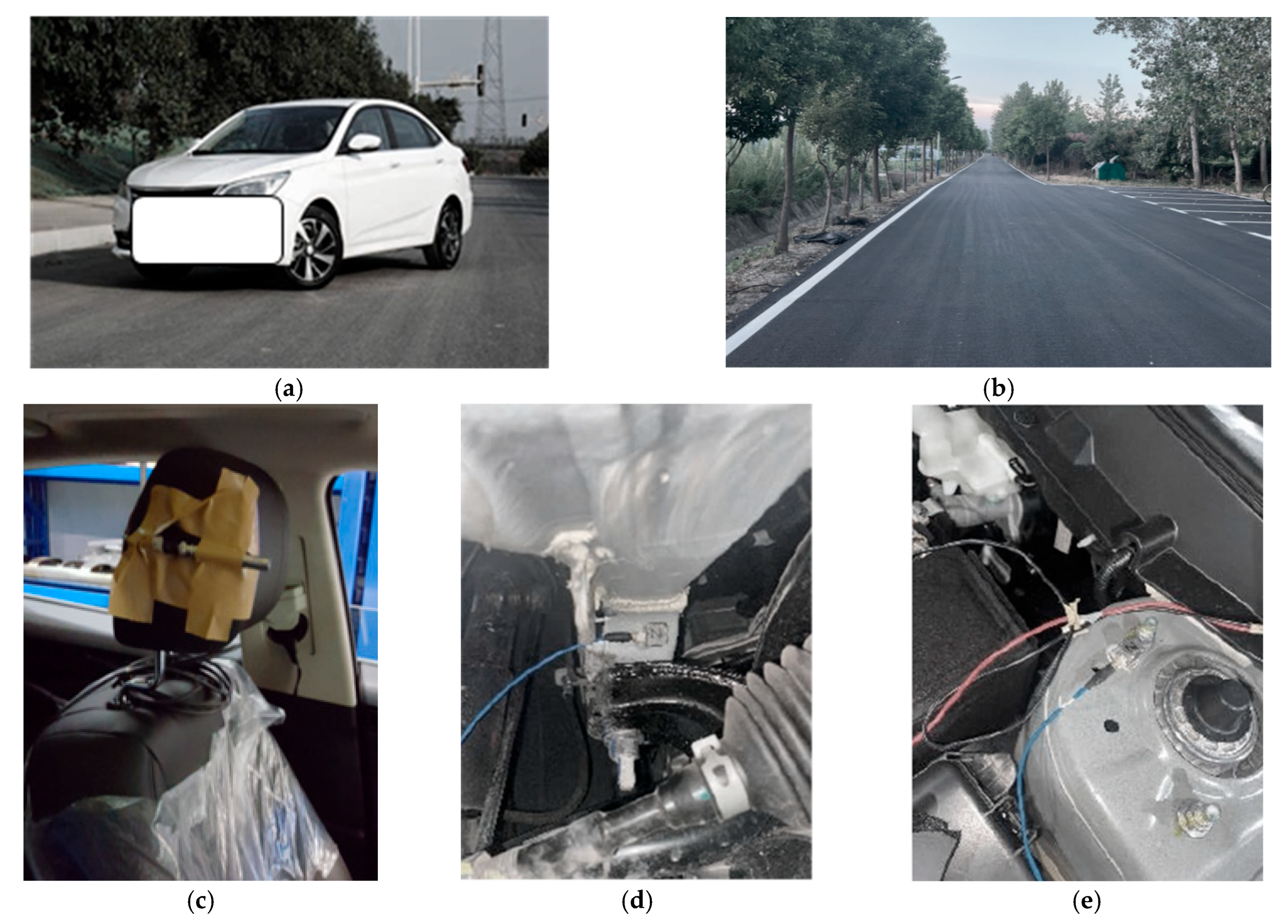
The tire noise test is carried out on rough asphalt pavement, mainly based on two main factors: Firstly, rough pavement serves as an effective catalyst for stimulating vehicle structure noise, while minimizing the influence of other extraneous noise sources, providing a more focused and reliable measure of the vehicle’s noise characteristics. Secondly, rough asphalt pavement is a common and representative road surface encountered in urban driving conditions. Therefore, conducting tests on such pavement ensures that the results more accurately reflect the real-world tire noise performance of vehicles under typical driving scenarios. The layout of some sensors is shown in Figure 5. PCB three-way vibration acceleration sensor is arranged at the front and rear steering knuckles on the left side of the vehicle to measure the vibration acceleration of the steering knuckle. A sound pressure sensor is strategically placed near the driver’s right ear to accurately measure the auditory experience within the vehicle’s cabin, and the sensor is oriented forward. It should be noted that the forward arrangement of the sound pressure sensor is based on the relevant provisions of GB/T18697-2002 ‘automotive interior noise measurement method’ [43].
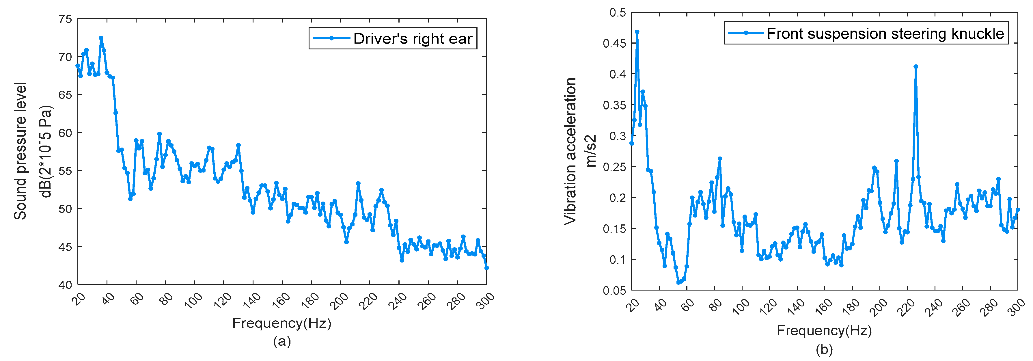
The driver’s right ear noise and the Z-direction vibration acceleration of the front suspension knuckle (i.e., vibration excitation) collected in the test are shown in Figure 6. In view of the fact that the spectrum of road structural noise predominantly occurs within the frequency range of 20 to 300 Hz, this study focuses on the vehicle interior noise data in this frequency range [44]. In addition, considering the correlation of the acoustic–vibration transfer characteristics, the frequency range of the vibration acceleration data is consistent with the noise data.

3.3. Data Augmentation

Due to the limitation of time and cost of the vehicle test, the number of valid data samples collected in this study is limited. In order to overcome this challenge, this study uses data augmentation techniques to expand the sample size. Data augmentation technology can achieve the analysis effect of more similar data by generating new data samples without significantly increasing the amount of data. In the field of data enhancement, it is mainly divided into two categories: nonlinear enhancement method and linear enhancement method. Nonlinear enhancement method examples include generative adversarial networks (GANs) [45] and variational autoencoders (VAEs) [46], generating new data samples by learning the distribution of training data. Although these methods can generate high-quality data samples, they usually require larger datasets and longer training time, which is not suitable for this study. In contrast, linear enhancement methods, such as Mixup, generate new data samples through simple linear interpolation, and have proven their effectiveness in multiple tasks [47,48,49]. Therefore, when dealing with vehicle vibration and noise data, this paper chooses the Mixup data enhancement strategy. There are two main reasons for choosing this strategy: First, the linear enhancement method preserves the fundamental structure of the data throughout the enhancement process, which is crucial for maintaining the physical characteristics of the vibration and noise data [50]. Secondly, by performing simple linear interpolation between the original samples, the Mixup method not only effectively increases the size and diversity of the dataset, but also prevents model overfitting and significantly improves the prediction ability of the model for unseen samples [51].
The Mixup approach creates new training samples by performing linear interpolation, represented by the following formula:
x ˜ = λ x i + ( 1 λ ) x j
y ˜ = λ y i + ( 1 λ ) y j
In the Mixup data augmentation method, (xi,yi) and (xj,yj) represent two samples randomly selected from the dataset, where x denotes the feature vector and y denotes the target value or label associated with these feature vectors. By linear interpolation between two samples, new training samples are generated. The feature vector x ˜ of the new sample is the weighted average of the original sample xi and xj, while the target value y ˜ of the new sample is the weighted average of yi and yj. The weight coefficient λ is a random number between 0 and 1, and its value follows the Beta distribution, that is, λ~Beta (α, β). By adjusting the value of λ, the Mixup method can change the position of the new sample in the original sample space. When the value of λ is large, the generated samples are closer to the original samples xi and yj. When the value of λ is small, the generated samples exhibit greater similarity to the original samples xj and yj. This method aims to make the generated new samples cover a wider range of original sample space, thereby increasing the diversity of training data and boosting the model’s flexibility and generalization capacity in response to data variations. For instance, using the driver’s ear noise measurement point as a reference, Figure 7 shows the distribution of new sample data points when λ = 0.2 and λ = 0.7. Through data enhancement technology, the original 20 groups of test samples were expanded to 300 groups.

4. Application and Verification of the Method

4.1. Development of a Tire Noise Prediction Model Using EINN

Before the super parameter setting of the CNN model, the input and output of the data sample need to be unified. The size of the input data is 30 × 141, where 30 represents the count of input features and 141 represents the frequency dimension of the input features, covering 20–300 Hz sequence data (frequency resolution is 2 Hz). The dimension of the output data is 1 × 141, that is, the interior noise, specifically at the driver’s right ear, was considered. From the total dataset, 210 samples were randomly selected as the training set, following a 7:3 ratio, while the remaining 90 samples were designated as the test set for model evaluation. The root mean square error (RMSE) was used to assess the model’s accuracy [52,53,54]. The training environment is Python 3.10, and the hardware is Intel Core i7-14700 KF processor, 64 GB memory and NVIDIA GeForce RTX 4060 Ti 16 G graphics card.
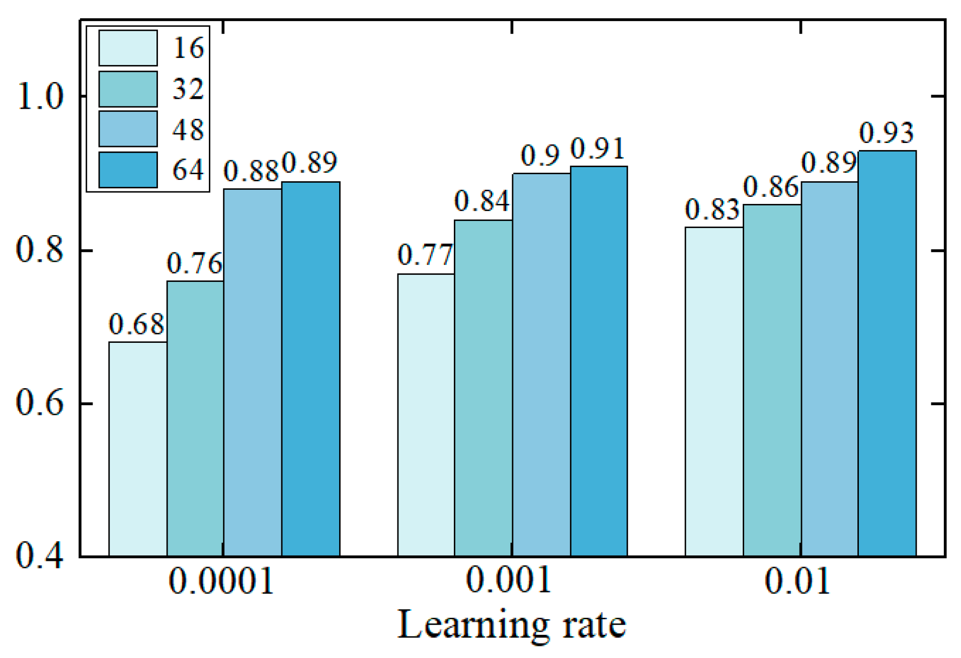
In this study, the grid search method is used to optimize the network parameters of EINN. The hyperparameters of the EINN mainly include the learning rate and the number of convolutional layer filters. The range of the learning rate is [0.001,0.01,0.1], and the range of filter number is [16,32,48,64]. Other parameters are as follows: the learning rate attenuation coefficient is 0.9, the batch size is 10, and the optimizer uses the adaptive momentum estimation (ADAM) gradient optimization algorithm, which combines the advantages of Momentum and RMSProp to achieve efficient search in the parameter space. According to the optimization grid, a total of 3 × 4 = 12 groups of training are performed, and each group of training presets 200 iterations to explore the model performance under different parameter configurations. By comparing the prediction accuracy of the model under different configurations, the optimal network parameter setting is finally determined: the highest model accuracy obtained is 0.944, the corresponding learning rate is selected as 0.001, and the number of hidden layer nodes is set to 48. The specific parameter optimization results are shown in Figure 8.
In addition, in the EINN, the setting of the three weight items ω has a significant impact on the network accuracy. Through numerical experiments, firstly, based on the unity of the magnitude of the three loss terms, the initial weight term is set to ω d = 1, ω p = 1, ω r = 1. In the follow-up, the changes in the three loss items in the training process of the fixed-weight strategy and the normalized adaptive weight strategy will be compared to optimize the weight allocation and enhance the model’s prediction accuracy.

4.2. EINN Model Comparison and Verification

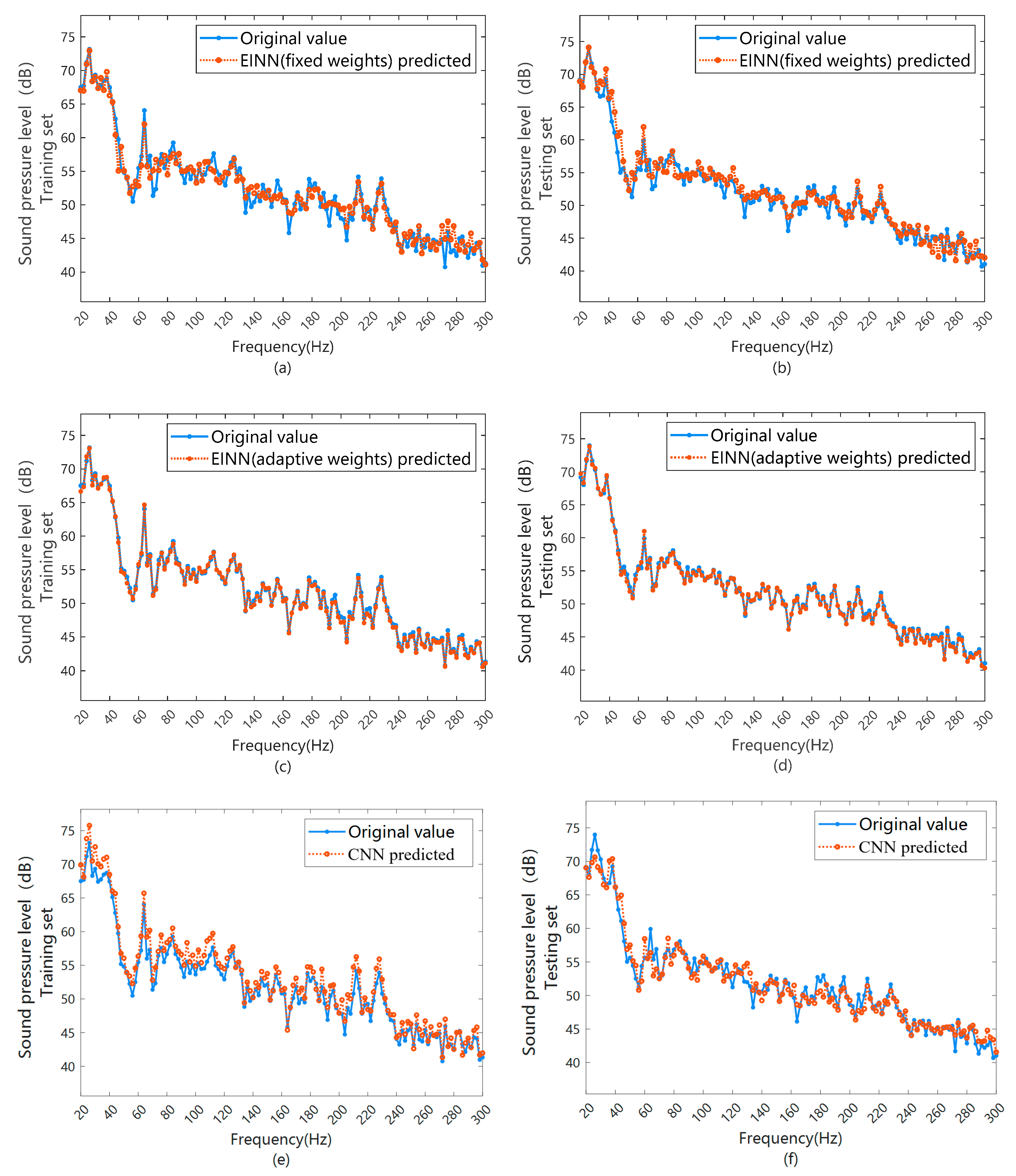
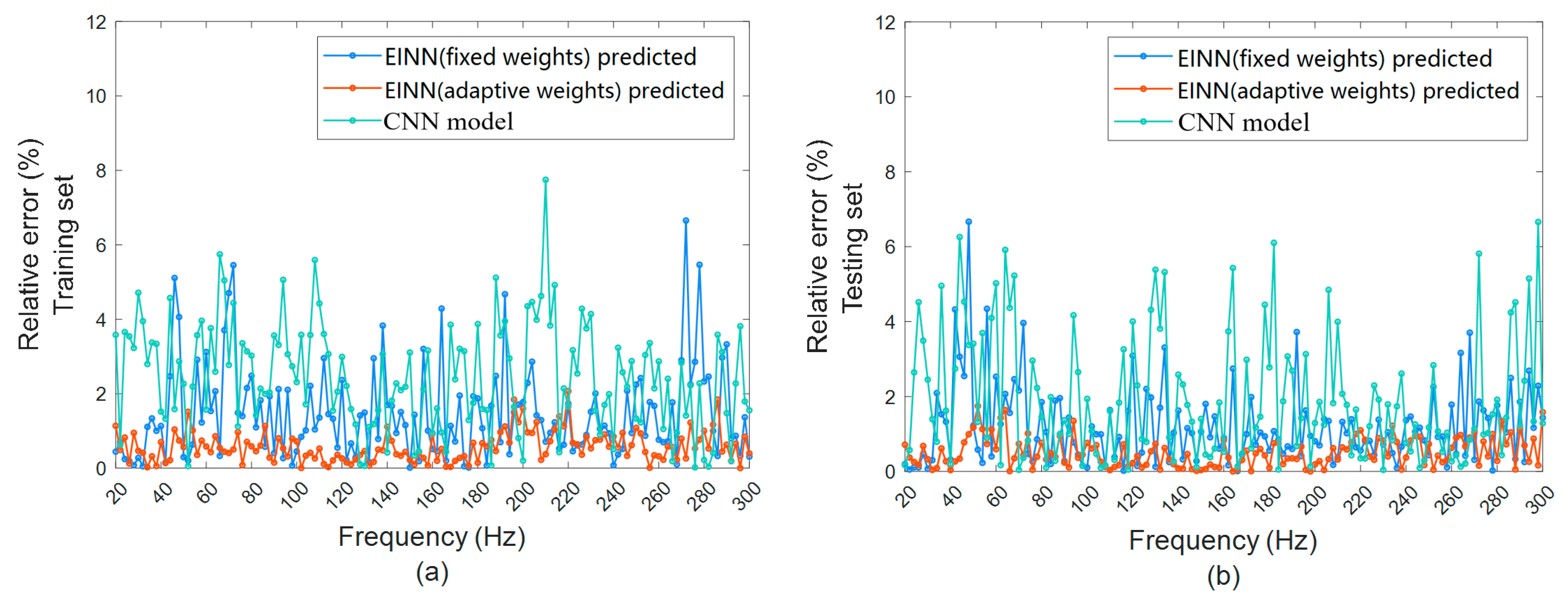
On the basis of the constructed model architecture, the EINN model is trained and compared with the fixed-weight EINN model and the traditional CNN model regarding model accuracy and processing efficiency. Figure 9 shows the prediction results of the three models under different frequency conditions. On the whole, the prediction curves of each model can better follow the change trend of the real value, indicating that the prediction results have certain engineering reliability. Further combined with the relative error results in Figure 10, the average relative error (MRE) of the CNN model in the training sets and the testing sets is 3.1% and 3.4%, respectively. The errors of the fixed-weight EINN model are 2.2% and 2.5%, respectively. The maximum relative error of the EINN model with normalized adaptive weight is only 1.2% and 1.4%. The results show that the proposed improved EINN model not only significantly reduces the error in predicting vehicle interior noise but also outperforms the comparison model in terms of fitting accuracy and generalization ability, reflecting stronger engineering applicability and advantages.
To thoroughly assess the performance of the EINN model in predicting vehicle interior noise, in addition to calculating MRE, the maximum relative error (MaxRE), average peak error (MPE) and maximum peak error (MaxPE) of the training set and test set were statistically analyzed. Among them, MPE is determined by calculating the relative error of the first five maximum peaks, and the specific results are shown in Table 1. From the comparison results, the model based on EINN is significantly better than the traditional CNN model in terms of model accuracy. Taking the test set as an example, compared with the CNN model, the fixed-weight EINN model has a 0.9% reduction in MRE and a 1.0% reduction in MaxRE. In addition, in terms of the fitting effect of peak frequency points, the fixed-weight EINN model performs more prominently, and MPE and MaxPE are 3.8% and 3.0% lower than CNN, respectively, reflecting its advantages in local feature capture. This result shows that the EINN model has stronger adaptability when dealing with data with significant peak characteristics and is of great significance for the prediction of specific frequency noise. Further, the performance of the model is significantly improved after the introduction of normalized adaptive weights. The MRE, MaxRE, MPE and MaxPE on the test set are 1.3%, 2.2%, 0.7% and 1.0%, respectively. The overall evaluation results show that the EINN model based on normalized weight not only has higher overall accuracy when predicting the actual tire noise level but is also superior to CNN and fixed-weight EINN models on the training set and validation set, showing stronger engineering application potential.
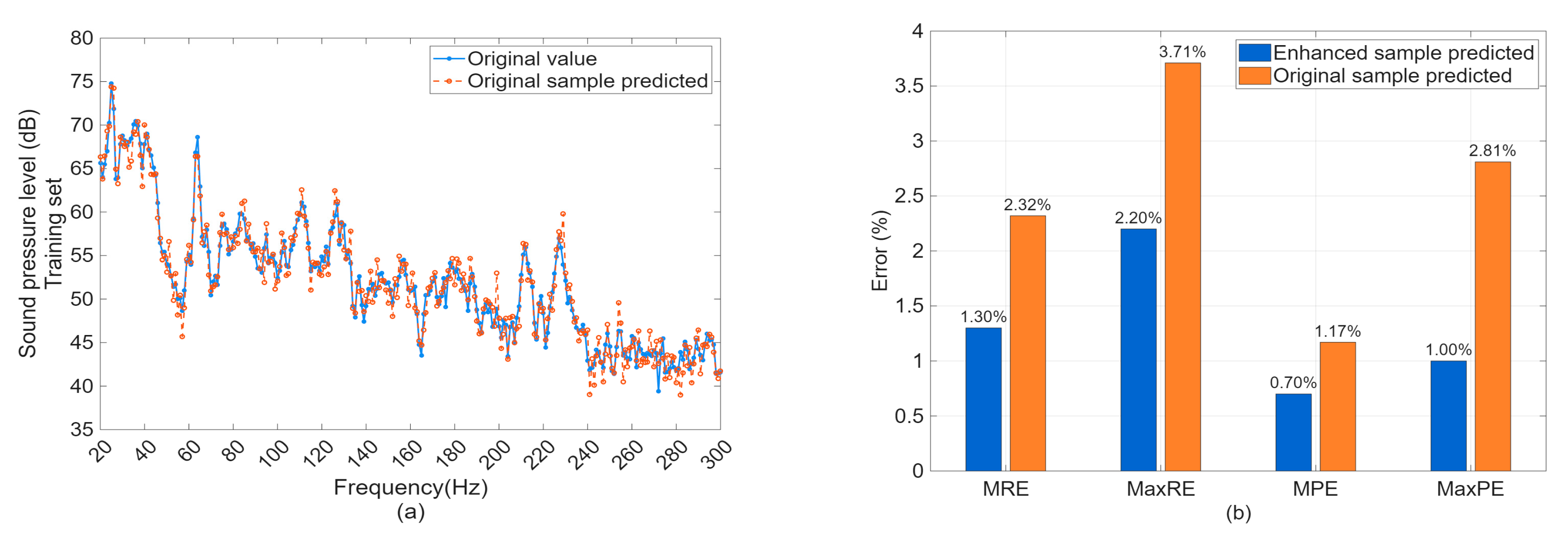
To thoroughly investigate the impact of data augmentation on model generalization, we conducted additional experiments. As shown in Figure 11, the EINN model (with adaptive weights) trained on only 20 original samples was compared with the EINN model (with adaptive weights) trained on an augmented dataset. The model trained on the augmented dataset achieved an MRE of 1.3% on test samples, lower than the model trained on original samples alone (MRE of 2.32%). This result demonstrates that Mixup augmentation not only increases the sample size but also enhances the model’s generalization ability by introducing meaningful variability. Future studies could further improve model performance by collecting larger-scale original datasets or exploring other augmentation methods.

5. Conclusions

This study introduces the EINN method to conduct a thorough investigation into the interior tire noise performance of vehicles, particularly within the 20–300 Hz frequency range. The EINN method combines both knowledge-based and data-driven approaches for noise prediction, leveraging the noise transfer relationship to enhance prediction accuracy. A key contribution of this work lies in embedding empirical vibro-acoustic mechanisms into the loss function, enabling the model to effectively integrate engineering knowledge with data, while an adaptive weight strategy is introduced to improve training robustness and numerical stability. By integrating these two methodologies, the model provides a more comprehensive analysis of how noise is transmitted and perceived inside the vehicle, which significantly improves the understanding and prediction accuracy of tire noise performance. In the comparative analysis with other models, the prediction accuracy of the EINN method at each frequency point is more than 92%, which outperforms the traditional CNN model by a significant margin. In addition, under the same hardware configuration and data volume conditions, the training time of the CNN model is 4.5 min per 150 epochs, while the EINN model takes only 3 min to complete the training, showing efficient training performance. The EINN method not only has achieved remarkable results in improving prediction efficiency and accuracy but also makes up for the shortcomings of traditional data-driven algorithms in interpretability. This method of combining knowledge and data provides a new idea for the efficient prediction of vehicle tire noise, provides an innovative solution to solve the tire noise problem, and provides a valuable reference for the modeling and analysis of similar complex systems. While the EINN method performs well in this study, it still has some limitations. Future work could extend this to larger and more diverse datasets to validate the EINN method’s generalization capabilities across different vehicle types and noise conditions. Furthermore, benchmark comparisons with other hybrid methods (such as LSTM/GRU or PINN variants) could be considered to further evaluate the relative advantages of the EINN method. Exploring the potential of the EINN method in higher frequency ranges or other NVH-related applications would also be a meaningful direction.
This study focuses on passenger pure electric vehicles with typical suspension and body structures; therefore, the results are directly applicable to similar passenger car platforms, while their extension to heavy vehicles such as lorries or trucks requires further validation.

Author Contributions

Writing—original draft preparation, P.D. and R.D.; conceptualization, H.H. methodology, Y.Y. and J.W.; software, P.D.; validation, J.W.; writing—review and editing, Y.Y.; visualization, P.D.; funding acquisition, W.D. All authors have read and agreed to the published version of the manuscript.

Funding

This research was funded by the SWJTU Science and Technology Project (No. R110222H01108).

Data Availability Statement

The original contributions presented in this study are included in the article. Further inquiries can be directed to the corresponding author.

Acknowledgments

The authors would like to acknowledge the support provided by the Institute of Energy and Power Research for the experimental research.

Conflicts of Interest

The authors declare no conflict of interest.

References

  1. Abidou, D.; Abdellah, A.H.; Haggag, S. Optimizing Rear Spoiler Angle for Enhanced Vehicle Braking Performance. SAE Int. J. Veh. Dyn. Stab. NVH 2025, 9, 10-09-04-0033. [Google Scholar] [CrossRef]
  2. Liu, K.; Liao, Y.; Wang, H.; Zhou, J. Road Noise Improvement Method for Battery Electric Vehicles Based on Bushing Stiffness Optimization. SAE Int. J. Veh. Dyn. Stab. NVH 2025, 9, 10-09-04-0032. [Google Scholar] [CrossRef]
  3. Zhu, H.; Zhao, J.; Wang, Y.; Ding, W.; Pang, J.; Huang, H. Improving of pure electric vehicle sound and vibration comfort using a multi-task learning with task-dependent weighting method. Measurement 2024, 233, 114752. [Google Scholar] [CrossRef]
  4. Li, X.; Lu, C.; Chen, W.; Zhu, Y.; Liu, Z.; Cheng, C.; Sun, M. A computationally efficient multichannel feedforward time–frequency-domain adjoint least mean square algorithm for active road noise control. Appl. Acoust. 2025, 231, 110441. [Google Scholar] [CrossRef]
  5. Raabe, J.; Fontana, F.; Neubeck, J.; Wagner, A. Contribution to the objective evaluation of combined longitudinal and lateral vehicle dynamics in nonlinear driving range. SAE Int. J. Veh. Dyn. Stab. NVH 2023, 7, 533–554. [Google Scholar] [CrossRef]
  6. Contartese, N.; Nijman, E.; Desmet, W. A procedure to restore measurement induced violations of reciprocity and passivity for FRF-based substructuring. Mech. Syst. Signal Process. 2022, 167, 108556. [Google Scholar] [CrossRef]
  7. Yuan, W.; Yang, Q. A Novel Method for Pavement Transverse Crack Detection Based on 2D Reconstruction of Vehicle Vibration Signal. KSCE J. Civ. Eng. 2023, 27, 2868–2881. [Google Scholar] [CrossRef]
  8. Huang, H.; Huang, X.; Ding, W.; Yang, M.; Fan, D.; Pang, J. Uncertainty optimization of pure electric vehicle interior tire/road noise comfort based on data-driven. Mech. Syst. Signal Process. 2022, 165, 108300. [Google Scholar] [CrossRef]
  9. Mikhailenko, P.; Piao, Z.; Kakar, M.R.; Bueno, M.; Athari, S.; Pieren, R.; Heutschi, K.; Poulikakos, L. Low-Noise pavement technologies and evaluation techniques: A literature review. Int. J. Pavement Eng. 2022, 23, 1911–1934. [Google Scholar] [CrossRef]
  10. Deubel, C.; Ernst, S.; Prokop, G. Objective evaluation methods of vehicle ride comfort—A literature review. J. Sound Vib. 2023, 548, 117515. [Google Scholar] [CrossRef]
  11. Dai, R.; Zhao, J.; Zhao, W.; Ding, W.; Huang, H. Exploratory study on sound quality evaluation and prediction for engineering machinery cabins. Measurement 2025, 253, 117684. [Google Scholar] [CrossRef]
  12. Huang, H.; Wang, Y.; Wu, J.; Ding, W.; Pang, J. Prediction and optimization of pure electric vehicle tire/road structure-borne noise based on knowledge graph and multi-task ResNet. Expert Syst. Appl. 2024, 255, 124536. [Google Scholar] [CrossRef]
  13. Chen, F.; Cao, Z.; Grais, M.E.; Zhao, F. Contributions and limitations of using machine learning to predict noise-induced hearing loss. Int. Arch. Occup. Environ. Health 2021, 94, 1097–1111. [Google Scholar] [CrossRef]
  14. He, X.; Chen, H.; Lv, C. Robust multiagent reinforcement learning toward coordinated decision-making of automated vehicles. SAE Int. J. Veh. Dyn. Stab. NVH 2023, 7, 475–488. [Google Scholar] [CrossRef]
  15. Raissi, M.; Perdikaris, P.; Karniadakis, G. Physics-informed neural networks: A deep learning framework for solving forward and inverse problems involving nonlinear partial differential equations. J. Comput. Phys. 2019, 378, 686–707. [Google Scholar] [CrossRef]
  16. Feng, Y.; Wang, W. Energy Equalities of the Inhomogeneous Navier-Stokes Equations, MHD Equations and Hall-MHD Equations. Bull. Malays. Math. Sci. Soc. 2025, 48, 166. [Google Scholar] [CrossRef]
  17. Feng, M.; Sun, T. Error analysis of a hybrid numerical method for optimal control problem governed by parabolic PDEs in random cylindrical domains. Adv. Comput. Math. 2025, 51, 22. [Google Scholar] [CrossRef]
  18. Yang, C.; Wang, J.; Jian, M.; Dai, J. Synchronization Control of Complex Spatio-Temporal Networks Based on Fractional-Order Hyperbolic PDEs with Delayed Coupling and Space-Varying Coefficients. Fractal Fract. 2024, 8, 525. [Google Scholar] [CrossRef]
  19. Jin, X.; Cai, S.; Li, H.; George, E. Nsfnets (navier-stokes flow nets): Physics-informed neural networks for the incompressible navier-stokes equations. J. Comput. Phys. 2021, 426, 109951. [Google Scholar] [CrossRef]
  20. Xu, Y.; Zhang, Y.; Lu, X. MADAN: A multi-angle domain adversarial network for robust cross-condition rolling bearing fault diagnosis. Meas. Sci. Technol. 2025, 36, 096101. [Google Scholar] [CrossRef]
  21. Schiassi, E.; Furfaro, R.; Leake, C.; Mario, D.; Johnston, H.; Mortari, D. Extreme theory of functional connections: A fast physics-informed neural network method for solving ordinary and partial differential equations. Neurocomputing 2021, 457, 334–356. [Google Scholar] [CrossRef]
  22. Cai, S.; Wang, Z.; Wang, S.; Perdikaris, P.; Karniadakis, G. Physics-Informed Neural Networks for Heat Transfer Problems. J. Heat Transf. 2021, 143, 060801. [Google Scholar] [CrossRef]
  23. Li, X.; Zhang, W. Physics-informed deep learning model in wind turbine response prediction. Renew. Energy 2022, 185, 932–944. [Google Scholar] [CrossRef]
  24. Chen, K.; Wu, G.; Peng, S.; Zeng, X.; Ju, L. The vehicle speed strategy with double traffic lights based on reinforcement learning. Int. J. Veh. Perform. 2023, 9, 250–271. [Google Scholar] [CrossRef]
  25. Zhang, X.; Yi, Y.; Wang, L.; Xu, Z.; Zhang, T.; Zhou, Y. Deep Neural Networks for Modeling Astrophysical Nuclear Reacting Flows. Astrophys. J. 2025, 990, 105. [Google Scholar] [CrossRef]
  26. Dai, R.; Zhao, J.; Sui, Q.; Zhao, W.; Ding, W.; Huang, H. Multi-dimensional evaluation and prediction of vibration comfort in electric loaders using ACO-Transformer. Sound Vib. 2025, 59, 3523. [Google Scholar] [CrossRef]
  27. Luo, D.; Yang, W.; Wang, Y.; Han, Y.; Liu, Q.; Yang, Y. Investigation of regenerative braking for the electric mining truck based on fuzzy control. Int. J. Veh. Perform. 2024, 10, 73–95. [Google Scholar] [CrossRef]
  28. Tonelli, R.; Buckert, S.; Patrucco, A.; Perez, B.B.; Gutierrez, J.; Sanchez, A. Electric Vehicle Ride & Vibrations Analysis: Full Electric Vehicle MBD Model Development for NVH Studies. SAE Int. J. Adv. Curr. Pract. Mobil. 2024, 7, 1024–1034. [Google Scholar] [CrossRef]
  29. Lawal, Z.; Yassin, H.; Lai, D.; Idris, A. Physics-informed neural network (PINN) evolution and beyond: A systematic literature review and bibliometric analysis. Big Data Cogn. Comput. 2022, 6, 140. [Google Scholar] [CrossRef]
  30. Leung, W.; Lin, G.; Zhang, Z. NH-PINN: Neural homogenization-based physics-informed neural network for multiscale problems. J. Comput. Phys. 2022, 470, 111539. [Google Scholar] [CrossRef]
  31. Marral, U.I.; Du, H.; Naghdy, F. Multidimensional Coupling Effects and Vibration Suppression for In-Wheel Motor–Driven Electric Vehicle Suspension Systems: A Review. SAE Int. J. Veh. Dyn. Stab. NVH 2025, 9, 229–251. [Google Scholar] [CrossRef]
  32. Soresini, F.; Barri, D.; Ballo, F.; Manzoni, S.; Gobbi, M.; Mastinu, G. Noise, Vibration, and Harshness Countermeasures of Permanent Magnet Synchronous Motor with Viscoelastic Layer Material. SAE Int. J. Veh. Dyn. Stab. NVH 2025, 9, 1–18. [Google Scholar] [CrossRef]
  33. Nicho, M.; Cusack, B.; McDermott, D.; Girija, S. Assessing IoT intrusion detection computational costs when using a convolutional neural network. Inf. Secur. J. A Glob. Perspect. 2025, 34, 471–491. [Google Scholar] [CrossRef]
  34. Hatami, M.; Gharaee, H.; Mohammadzadeh, N. SADCNN: Supervised anomaly detection based on convolutional neural network models. Inf. Secur. J. A Glob. Perspect. 2025, 34, 455–470. [Google Scholar] [CrossRef]
  35. Hamrouni, C.; Alutaybi, A. Modeling and predicting the transmission efficiency of communication devices under joint noise and vibration disturbances. Sound Vib. 2025, 59, 2112. [Google Scholar] [CrossRef]
  36. Alutaybi, A.; Hamrouni, C. Impact of vibration on wind turbine efficiency and LSTM-based power conversion prediction. Sound Vib. 2025, 59, 2059. [Google Scholar] [CrossRef]
  37. Tian, J.; Wang, H.; He, J.; Pan, Y.; Cao, S.; Jiang, Q. Learning and interpreting gravitational-wave features from CNNs with a random forest approach. Mach. Learn. Sci. Technol. 2025, 6, 035045. [Google Scholar] [CrossRef]
  38. Elabd, E.; Hamouda, M.H.; Ali, M.; Fouad, Y. Correction: Climate change prediction in Saudi Arabia using a CNN GRU LSTM hybrid deep learning model in al Qassim region. Sci. Rep. 2025, 15, 31371. [Google Scholar] [CrossRef]
  39. Jin, M.; Zuo, S.; Wu, X.; Li, S.; Li, H.; Shi, L.; Chen, Y. Multistage operation transfer path analysis of an electric vehicle based on the regularization of total least squares. Mech. Syst. Signal Process. 2025, 225, 112250. [Google Scholar] [CrossRef]
  40. Elliott, A.S.; Moorhouse, A.T.; Huntley, T.; Tate, S. In-situ source path contribution analysis of structure borne road noise. J. Sound Vib. 2013, 332, 6276–6295. [Google Scholar] [CrossRef]
  41. Pu, Z.; Yi, J.; Liu, Z.; Qiu, T.; Sun, J.; Li, F. A review of research on group intelligent decision-making methods driven by knowledge and data synergy. J. Autom. 2022, 48, 1–17. [Google Scholar] [CrossRef]
  42. Liu, W.; Zhang, X.; Wang, Z.; Wang, Y.; Hu, B.; Zhuang, Y. Exploration of Vibration Signal Measurement Method of Automobile Parts Utilizing FPGA/Photoelectric Sensor. J. Nanoelectron. Optoelectron. 2021, 16, 1629–1637. [Google Scholar] [CrossRef]
  43. GB/T 18697-2002; Acoustics—Method for Measuring Vehicle Interior Noise. General Administration of Quality Supervision, Inspection and Quarantine of the People’s Republic of China, Standardization Administration of the People’s Republic of China: Beijing, China, 2002.
  44. Shields, M.; Zhang, J. The generalization of Latin hypercube sampling. Reliab. Eng. Syst. Saf. 2015, 148, 96–108. [Google Scholar] [CrossRef]
  45. Huang, H.; Huang, X.; Ding, W.; Yang, M.; Yu, X.; Pang, J. Vehicle vibro-acoustical comfort optimization using a multi-objective interval analysis method. Expert Syst. Appl. 2023, 213, 119001. [Google Scholar] [CrossRef]
  46. Pan, Z.; Yu, W.; Yi, X.; Khan, A.; Yuan, F.; Zheng, Y. Recent progress on generative adversarial networks (GANs): A survey. IEEE Access 2019, 7, 36322–36333. [Google Scholar] [CrossRef]
  47. Huang, J.; Yang, P.; Xiong, B.; Lv, Y.; Wang, Q.; Wan, B.; Zhang, Z.Q. Mixup-based data augmentation for enhancing few-shot SSVEP detection performance. J. Neural Eng. 2025, 22, 046038. [Google Scholar] [CrossRef] [PubMed]
  48. Tang, L.; Zhang, Z.; Yang, J.; Yong, F.; Wang, Q.; Sun, S.; Shao, H. Intervention-based Mixup Augmentation for Multiple Instance Learning in Whole-Slide Image Survival Analysis. IEEE Trans. Med. Imaging 2025. [Google Scholar] [CrossRef]
  49. Cao, K.; Peng, J.; Chen, J.; Hou, X.; Ma, J. Adversarial Style Mixup and Improved Temporal Alignment for Cross-Domain Few-Shot Action Recognition. Comput. Vis. Image Underst. 2025, 255, 104341. [Google Scholar] [CrossRef]
  50. Kwon, S.; Lee, Y. Explainability-based mix-up approach for text data augmentation. ACM Trans. Knowl. Discov. Data 2023, 17, 1–14. [Google Scholar] [CrossRef]
  51. Guo, H. Nonlinear mixup: Out-of-manifold data augmentation for text classification. Proc. AAAI Conf. Artif. Intell. 2020, 34, 4044–4051. [Google Scholar] [CrossRef]
  52. Kalange, N. Prediction of Stock Prices Using LSTM-ARIMA Hybrid Deep Learning Model. Asian J. Probab. Stat. 2025, 27, 28–39. [Google Scholar] [CrossRef]
  53. Tempone, G.; de Carvalho Pinheiro, H.; Imberti, G.; Carello, M. Control System for Regenerative Braking Efficiency in Electric Vehicles with Electro-Actuated Brakes. SAE Int. J. Veh. Dyn. Stab. NVH 2024, 8, 265–284. [Google Scholar] [CrossRef]
  54. Yang, M.; Dai, P.; Yin, Y.; Wang, D.; Wang, Y.; Huang, H. Predicting and optimizing pure electric vehicle road noise via a locality-sensitive hashing transformer and interval analysis. ISA Trans. 2025, 157, 556–572. [Google Scholar] [CrossRef] [PubMed]
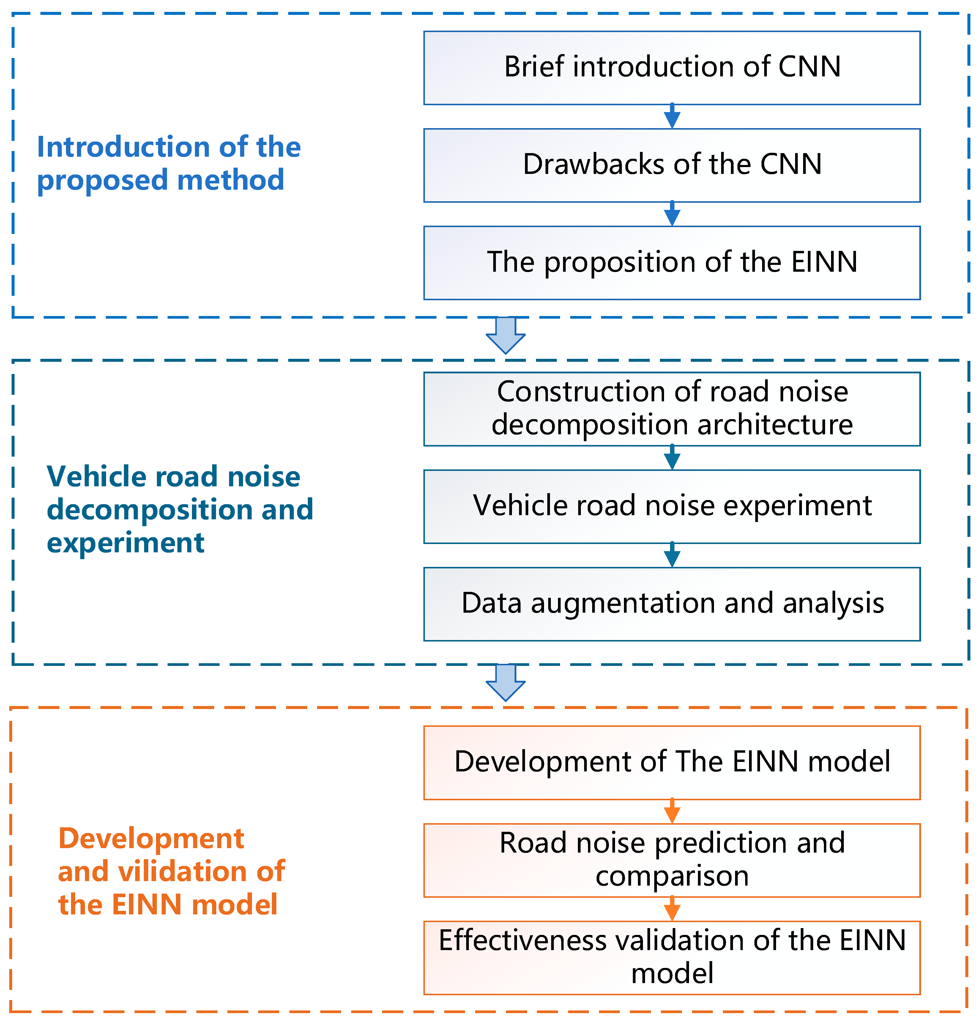
Figure 1. The technical route of vehicle pavement structure noise prediction method based on EINN.
Machines 13 00911 g001
Figure 2. CNN topology structure with input, convolution, pooling and fully connected layers for road noise feature extraction and prediction.
Machines 13 00911 g002
Figure 3. EINN architecture based on CNN, incorporating the empirical constraint module to integrate physical knowledge and improve road noise prediction accuracy.
Machines 13 00911 g003
Figure 4. Analysis of tire noise influencing factors and performance decomposition.
Machines 13 00911 g004
Figure 5. Road test combination diagram. (a) The tested vehicle; (b) the tested road surface; (c) the microphone on the driver’s seat; (d) the acceleration sensor on the subframe; (e) the acceleration sensor on the shock absorber top mount.
Machines 13 00911 g005
Figure 6. Vehicle tire noise road test data. (a) Driver’s right ear noise; (b) front suspension steering knuckle acceleration.
Machines 13 00911 g006
Figure 7. Driver’s right ear noise enhancement data schematic. (a) Augmentation sample 1# (λ = 0.2); (b) augmentation sample 2# (λ = 0.7).
Machines 13 00911 g007
Figure 8. Network search parameter optimization results.
Machines 13 00911 g008
Figure 9. Driver’s right ear noise training and testing results. (a) EINN (fixed weight) training results. (b) EINN (fixed weight) testing results. (c) EINN (fixed weight) training results. (d) EINN (fixed weight) testing results. (e) CNN training results. (f) CNN testing results.
Machines 13 00911 g009
Figure 10. The relative error of training and testing of the driver’s right ear noise prediction model. (a) Training set; (b) testing set.
Machines 13 00911 g010
Figure 11. Performance of the EINN model on test samples. (a) Predictions of the EINN model trained on original samples. (b) Error comparison between the EINN model trained on original samples and the EINN model trained on augmented samples.
Machines 13 00911 g011
Table 1. Comparison of prediction accuracy of three prediction methods.
MREMaxREMPEMaxPE
EINN
(Fixed weight)
Training2.2%6.3%2.3%3.3%
Testing2.5%5.8%2.1%3.4%
EINN
(Adaptive weight)
Training1.1%2.0%0.8%1.0%
Testing1.3%2.2%0.7%1.0%
CNNTraining3.0%7.5%5.8%5.9%
Testing3.4%6.8%5.9%6.4%
Disclaimer/Publisher’s Note: The statements, opinions and data contained in all publications are solely those of the individual author(s) and contributor(s) and not of MDPI and/or the editor(s). MDPI and/or the editor(s) disclaim responsibility for any injury to people or property resulting from any ideas, methods, instructions or products referred to in the content.