Abstract
This study investigates the transverse loads acting on high-speed train bogie frames under actual service conditions. To enable direct identification, the locating arms were instrumented as bending sensors and calibrated under realistic lateral-stop constraints, ensuring robustness of the measurement channels. Field tests were conducted on a CR400BF high-speed EMU over a 226 km route at six speed levels (260–390 km/h), with gyroscope and GPS signals employed to recognize typical operating conditions, including straights, curves, and switches (straight movement and diverging movements). The results show that the proposed recognition method achieves high accuracy, enabling rapid and effective identification and localization of typical operating conditions. Under switch conditions, the bogie frame transverse loads are characterized by low-frequency, large-amplitude fluctuations, with overall RMS levels being higher in diverging switches and straight-through depot switches. Curve parameters and speed levels exert significant influence on the amplitude of the transverse-load trend component. On curves with identical parameters, the trend-component amplitude exhibits a quadratic nonlinear relationship with train speed, decreasing first and then increasing in the opposite direction as speed rises. In mainline curves and straight sections, the RMS values of transverse loads on Axles 1 and 2 scale proportionally with speed level, with the leading axle in the direction of travel consistently producing higher transverse loads than the trailing axle. When load samples are balanced across both running directions, the transverse load spectra of Axles 1 and 2 at the same speed level show negligible differences, while the spectrum shape index increases proportionally with speed level.
1. Introduction
By the end of 2024, the operational mileage of China’s high-speed rail reached 48,000 km. High-speed trains are a key component of the system. Currently, China’s high-speed EMU products cover speeds of 250 km/h, 300 km/h, and 350 km/h and are capable of meeting the demands of vast geographical areas, complex and diverse environments, as well as long-distance and high-intensity operations, injecting strong momentum into the rapid development of the economy and society. Meanwhile, this has also raised higher requirements for accurately assessing the fatigue strength of structural components in different types of vehicles.
As the running gear of high-speed trains, the bogie plays a crucial role in the train’s movement, steering, traction, and braking, making it a key component that determines the operational safety and performance of high-speed trains. The components of the bogie are illustrated in Figure 1. The bogie frame, as one of the most important load-bearing structures in the running assembly, bears and transmits various loads from the car body, wheelsets, and its own suspension components. Its service performance is vital to the operational safety of high-speed trains. Currently, the structural design and reliability evaluation of the bogie frame typically rely on load conditions specified in international standards, such as EN 13749 [1], UIC 615-4 [2], and JIS E 4207 [3]. However, due to significant variations in track environments and operating conditions, these international load standards are not fully applicable to the reliability assessment of bogie frames for high-speed trains across different regions. On the one hand, the frame may meet the evaluation standards during the design phase, but fatigue failure can still occur during service. On the other hand, since international standards are designed for broad applicability, utilizing the load conditions specified in these standards for fatigue strength evaluation of the frame often results in excessive conservatism, which becomes a bottleneck in the lightweight design of the frame. Load conditions form the foundation for structural design and reliability evaluation. It is, therefore, essential to accurately determine the actual load conditions for the bogie frame under different operational conditions and to conduct structural design and reliability assessments based on these conditions.
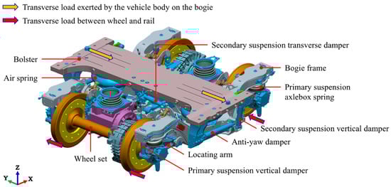
Figure 1.
A typical high-speed train bogie frame system and its transverse load.
The structural form, material mechanical properties, and load boundary conditions are key factors determining the structural fatigue strength. Accurately identifying the loads acting on the frame during the vehicle’s actual operation and conducting related research are of great significance for properly evaluating the frame’s fatigue strength, enhancing the structural reliability of the frame, and ensuring the safe operation of the vehicle [4,5,6].
The identification and measurement methods for structural dynamic loads are generally divided into two types: indirect testing methods and direct testing methods [7]. Indirect testing methods are suitable for situations where external loads are difficult to measure directly. These methods infer structural dynamic loads by indirectly measuring the structural responses (such as displacement, velocity, and acceleration responses). This typically involves issues such as the ill-conditioning of the system transfer matrix, the selection of the positions of the identification points, and calculation accuracy and stability, and such methods face various constraints in practical engineering applications. Direct testing methods, on the other hand, use force sensors to directly measure the structural loads and are suitable for situations where the loads are well-defined and can be directly tested.
The bogie frame is a typical large structure that bears multi-source load systems and exhibits significantly low damping characteristics. Indirectly identifying loads through the frame’s response is prone to divergence in computational results due to the ill-conditioning of the load–response transfer matrix. Additionally, the bogie frame load-testing cycle is long, and the data volume is enormous. Inversion calculations for dynamic loads are inefficient, and it is difficult to ensure identification accuracy. Therefore, strain gauges are commonly applied to the bogie frame and its connecting components, enabling direct testing of frame loads through strain-gauge measurements.
In recent years, many scholars have focused on identifying dynamic loads acting on bogie frames of high-speed trains under actual operating conditions while conducting research on load characteristics and fatigue damage. Ren et al. [8,9,10,11] identified the vertical load of axle box spring, the transverse load of locating node, and the local load of motor, gear box, anti-roll torsion bar, traction rod, brake lift, and other components of high-speed EMUs, analyzed the time domain, frequency domain, and statistical characteristics of each load, and explored the contribution of each load to fatigue damage of the frame. Zhang et al. [12] used axle box spring and primary shock absorber force sensor to identify vertical load of the frame, and compiled stress spectrum to analyze fatigue damage distribution of bogie frame according to load–stress transfer relationship. Ji et al. [13] analyzed the time domain, frequency domain, and load value distribution characteristics of the measured torsion loads of two different bogie frames, evaluated the similarity of the torsion load spectrum, and verified the feasibility of the interoperability of the torsion load spectrum of two different bogie frames based on fatigue damage simulation. Gao [14] identified the bogie frame load in the high-cold environment based on the load–stress transfer matrix and the measured dynamic stress of the line and explored the evolution law of the framework load. Wu and Ren [15] developed a high-precision force measurement frame and used genetic algorithm-based spectrum calibration to match measured damage in metro bogie frames, yielding a validated load spectrum for fatigue reliability design. Li et al. [16] proposed a load phase matrix reconstruction method that restored phase information lost during rain-flow counting, yielding a calibrated spectrum that more accurately reflected measured fatigue damage of metro bogie frames. Zhang et al. [17] investigated the fatigue failure of bogie-frame lifeguards and showed, through field tests and numerical simulation, that rail-corrugation-induced resonance significantly shortens their service life, suggesting rail grinding and structural improvements as mitigation measures. Wu et al. [18] developed an online method to estimate bogie frame fatigue damage by deriving transfer functions between axle box accelerations and frame stresses, enabling frequency-domain life prediction and supporting condition-based maintenance of metro vehicles. Transverse load is one of the main loads that the frame bears and has an important impact on fatigue damage to the overall structure of the bogie frame. However, few existing studies involve transverse loads of the bogie frame, and there is a lack of systematic analysis of these loads.
The load characteristics are closely related to the vehicle operating conditions and environment. Tao et al. [19] took the CR-400-AF high-speed EMU bogie frame structure as the research object. Based on the long-term line test data from the Beijing–Shanghai High-Speed Railway and by studying the variation in loads with the vehicle’s operating speed, a discrete load spectrum for the bogie frame structure was developed. Zhang [20] used the bogie frame loads and measured damage data of high-speed EMUs at speed levels ranging from 240 km/h to 380 km/h on the Zhengzhou–Xuzhou Passenger Dedicated Line. By fitting the load spectrum distribution, a functional relationship between the frame loads and speed was established, thereby obtaining the bogie frame load spectrum for a speed of 400 km/h. Su [21] analyzed the effects of train operating speed, up and down line conditions, and wheelset re-profiling on the characteristics of the loads.
Many scholars have conducted extensive research on the identification methods of high-speed train operating conditions and applied the load identification results from various operating conditions to the establishment of load spectra. Qiao [22] identified the operating conditions of high-speed trains based on the multi-scale entropy of the measured load signal of the bogie frame, and this method significantly improved the identification effect of switch operating conditions. Based on gyroscope and GPS signals, Zhang [23] uses empirical mode decomposition and energy entropy to identify the operating conditions of high-speed trains and studies the fatigue damage of the framework under different operating conditions. Chen et al. [24,25] developed railway condition recognition software and compiled the standardized load spectrum of a high-speed train bogie frame on the basis of analyzing the load characteristics of the frame under different conditions. Rao [26] and Guo [27] identified fault conditions of high-speed trains based on multi-view clustering integration and deep learning classification integration, respectively. Although the above working condition identification methods have good results, they mostly involve complex signal processing processes and are not convenient for engineering applications. Zou [28] conducted research on the bogie frame load spectrum of intercity EMUs and established a load spectrum model based on actual line-measured loads and dynamic stresses. Wang [29] investigated the load characteristics of the line under actual operating conditions and established the relationship between line loads and structural fatigue damage.
Most prior studies on load identification have mainly focused on vertical and torsional loads, while systematic and generalizable research on transverse and other types of loads remains limited. The present study addresses this gap by proposing a new method for transverse load identification and analyzing load characteristics under different operating conditions.
In this study, we develop a direct transverse-load identification scheme by instrumenting locating arms with bending cells and performing bi-directional, as-installed calibration under realistic lateral-stop constraints. Building on this, gyroscope and GPS signals are employed to identify four typical operating conditions of high-speed trains: straight lines, curves, and straight/diverging movements through switches. Taking the load–time history as the research object and combining it with gyroscope signals and train operating attitude, we systematically analyze the time- and frequency-domain characteristics of transverse loads under these conditions. Furthermore, the root mean square (RMS) and trend amplitude of transverse loads under different track conditions are calculated and statistically analyzed to comprehensively characterize amplitude fluctuations. Finally, a 16-level, speed-resolved rain flow spectrum is constructed from long-distance in-service tests, providing a validated basis for fatigue assessment and standard localization.
This paper is organized as follows: Section 2 presents the load identification methods, test lines, and test speed levels. Section 3 introduces an identification method for four typical operating conditions—straight lines, curve lines, and switches (including straight movement and diverging movement through switches)—based on gyroscope and GPS signals. Section 4 focuses on the load-time history of the upward line, analyzing the time-domain and frequency-domain characteristics of transverse loads. Section 5 statistically analyzed the impact of factors such as line conditions and operating conditions on the time-domain and frequency-domain characteristics of transverse loads, establishing a transverse load spectrum for different speed levels. Section 6 discusses and summarizes the conclusions of this study.
2. Transverse Load Calibration and Measurement
2.1. Transverse Load Description
The composition of a typical high-speed train bogie system is shown in Figure 2. The bogie frame is connected to the wheelset through primary suspension components and locating arms, and to the bolster (belonging to the vehicle body) through a series of secondary suspension system components. During the operation of the train, especially when passing through curve-line or switch sections, there is a relative transverse movement between the car body and the bogie. The bogie bears the transverse load from the car body, which is balanced by the transverse load generated when the rail and wheel contact are transmitted by the locating arms. At this point, the bogie frame is subjected to transverse loads, the magnitude and direction of which depend on the actual line conditions and the constantly changing wheel–rail interaction over time.
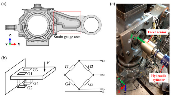
Figure 2.
Load channels calibration. (a) Strain gauges position. (b) Bending cell. (c) Transverse load application.
2.2. Load Channels Calibration
The locating arm is a key bearing component in the transverse load transmission path, so it is modified into a sensor to directly identify the transverse loads acting on the bogie frame. When the bogie frame is subjected to transverse load, the locating arm bends relative to the node where it connects to the bogie frame (referred to as the locating arm node), which can be simplified as a cantilever beam model under concentrated load.
To achieve load decoupling identification and improve testing accuracy, each locating arm is instrumented with a bending cell composed of four strain gauges, featuring axial load compensation, as shown in Figure 2a,b. During the load channel coefficient calibration, the locating arm is installed in the bogie frame according to the actual applying state. The constraint is applied at the lateral stop, and the transverse load of the same direction is applied stepwise at the two axle ends, as shown in Figure 2c. After linear fitting, the calibration coefficient of the load identification bridge of each locating arm is obtained. To reduce the calibration error, the final calibration coefficient is taken as the absolute average of the calibration results of the two directions. The positive and negative signs are determined according to the calibration direction. In actual tests, the ratio of the output strain value from each locating arm load identification bridge to its calibration coefficient is the transverse load on the frame by the axle where it is located. To further reduce the test error, the average value of the time domain load identification results of the two locating arms on the same axle is taken as the transverse loads from each axle that the bogie frame bears.
2.3. Track Test
The calibrated locating arms are mounted on the power bogie of the MH04 car for transverse load track testing. As shown in Figure 3, after departing from Zhengzhou East EMU Depot, the test train conducted multiple round-trip tests on the Kaifeng North Station–Xiaoxian North Station trial section without intermediate stops and finally returned to Zhengzhou East EMU Depot upon test completion. The EMU depot’s internal track length is 9.3 km, while the test section spans 226.3 km. The train’s maximum operating speed is 80 km/h in the EMU depot zone, while the operating speed in the test section covers six graded speed levels, including 260 km/h, 280 km/h, 310 km/h, 330 km/h, 350 km/h, and 390 km/h.
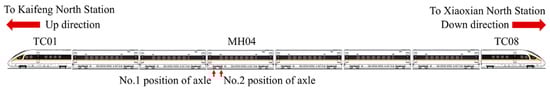
Figure 3.
Test train and operational information.
For the convenience of data analysis and operational condition identification, a GPS and a gyroscope were installed on the carbody above the tested bogie to obtain the vehicle’s operating speed, position, and motion states. The complete datasets were acquired under the typical track conditions, including straight-line sections, curve-line sections, and switches throughout the testing process.
The eDAQ dynamic data acquisition system is used to continuously collect a variety of data at the same time. The sampling frequency of the transverse load and gyroscope signal is 500 Hz, and the sampling frequency of the GPS signal is 50 Hz, which meets the requirement of the frequency range of the dynamic response signal and ensures the authenticity of the test data.
3. Typical Operating Condition Identification
This study performs identification and localization of train passage under four typical operating conditions—straight-line section, curve-line section, and switches (including both diverging and straight movement)—based on gyroscope and GPS signals, and determines detailed curve parameters using track maintenance data.
3.1. Time-Domain Characteristics of Gyroscope Signal
The track testing system employs a microelectromechanical triaxial gyroscope based on the Coriolis acceleration principle, which simultaneously measures the rotational angular velocities of the vehicle body around the X, Y, and Z axes during motion, corresponding to the roll, pitch, and yaw movements, respectively. The roll and yaw angular velocity signals from the gyroscope are used for operating condition identification after detrending and applying a 0.5 Hz low-pass filter.
Figure 4a shows the gyroscope signals as the train passes through straight-line and curve-line sections. When the train runs on the straight-line section, the vehicle body remains relatively stable, and the roll and yaw angular velocity signals fluctuate slightly around zero.
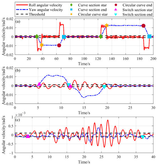
Figure 4.
Time-domain gyroscope signals under typical operational conditions. (a) Passing through straight-line and curve-line sections. (b) Diverging movement over switch. (c) Straight movement over switch.
In order to prevent the inertial centrifugal force from suddenly appearing or disappearing when the vehicle enters or exits a curve-line section, reduce the impact force between the high rail wheel and the high rail, and maintain smooth vehicle operation within the curve-line section, a transition curve with gradually varying curvature radius and high rail superelevation is set between the straight-line section and the curve-line section. This transition curve has the following characteristics [30]:
- (1)
- The radius decreases gradually from infinite (corresponding to the straight section) to the radius R of the circular curve (or increases from R to infinite);
- (2)
- The gauge widening of the inner rail gradually increases from zero to the full widening value on the circular curve (or gradually decreases from the full circular curve widening value back to zero);
- (3)
- The outer rail superelevation increases gradually from zero on the straight section to the superelevation value at the circular curve (or decreases from the curve’s superelevation to zero).
China’s high-speed railway adopts a cubic parabola transition curve and preferably chooses a linear superelevation ramp. The design requirement specifies that the angular velocity of vehicle roll at the start and end points of the transition curve is zero, and that the angular velocity varies continuously at intermediate points [30,31].
Based on the characteristics and technical requirements of the curve-line section, as shown in Figure 4a, when the train passes through a curve-line section, the amplitude of the yaw angular velocity signal gradually increases along the transition curve and remains stable after entering the curve-line section. Its amplitude and duration are related to the curve radius and the length of the curve-line section.
As the train exits the curve-line section via another transition curve, the amplitude of yaw angular velocity gradually decreases to near zero. On the other hand, the roll angular velocity signal increases from near zero along the transition curve, then decreases back to near zero, and fluctuates slightly around zero within the curve-line section.
Meanwhile, the direction of the curve (left/right turn) can be determined based on the positive/negative sign of the gyroscope signal. Taking the yaw angular velocity as an example, a positive value indicates that the vehicle body is deflecting to the left relative to the direction of travel, corresponding to a left-hand curve, and vice versa.
During the process of entering or exiting a high-speed train depot or station, it typically passes through a switch section, which can be categorized into two scenarios: diverging movement and straight movement. The corresponding gyroscope signals are shown in Figure 4b,c. According to the Design Specification for High-Speed Railway [32], a No. 18 high-speed switch, allowing for an operating speed of 80 km/h in a diverging movement section, is used to connect the main line and arrival–departure tracks. Inside the high-speed train depot, No. 12 or No. 9 switches are used, allowing for operating speeds of 50 km/h and 35 km/h in diverging movement, respectively. When the train passes over a diverging movement section, it passes over a small-radius curve within the switch, causing the vehicle body to yaw toward one side of the travel direction. The yaw angular velocity signal from the gyroscope exhibits characteristics similar to those observed in curve-line sections, while the roll angular velocity shows continuous large-amplitude fluctuations. When the train passes through the switch in the straight movement, the yaw angular velocity shows no significant variation, while the roll angular velocity exhibits continuous and pronounced fluctuations due to the complex geometry of the switch section.
3.2. Condition Identification Method
Typical operating situations are identified based on the time-domain amplitude variation characteristics of gyroscope signals. The identification process is illustrated in Figure 5, with the key steps described as follows:
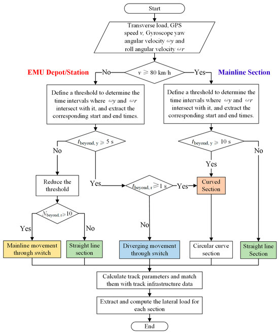
Figure 5.
Condition identification process.
- (1)
- According to the diverging movement operating speed (80 km/h) of the single switch connecting the mainline section and arrival–departure tracks, the input signals are divided into two segments: those corresponding to the mainline sections, stations, and high-speed train depots;
- (2)
- By setting appropriate upper and lower threshold values (±1 × 10⁻³ rad/s) for the mainline gyroscope signal, the start and end moments of the switch sections are determined when the gyroscope signal intersects the thresholds. The type of track sections (curve-line or straight-line) is determined based on the duration tbeyond,y, for which the yaw angular velocity signal exceeds the defined threshold range. The start and end times, as well as the number of such sections, are recorded accordingly. Within a curve-line section, the first and last moments at which the roll angular velocity signal intersects the threshold are identified as the start and end times of the circular curve-line section;
- (3)
- A similar procedure is applied to the gyroscope signals within the station. The existence of a transition curve is determined based on tbeyond,y, and the durations for which the first and last roll angular velocity signal exceed the threshold within a curve-line section (tbeyond1,r and tbeyond2,r, respectively). This allows for distinguishing between a regular curve-line section and a diverging movement section. The start and end times of each curve-line section and diverging movement section, along with the total number of occurrences, are recorded accordingly;
- (4)
- If tbeyond,y does not meet the required duration threshold, the upper and lower threshold range is reduced (set to ± 1 × 10⁻⁴ rad/s). Then, based on the number of consecutive peak and trough values of the roll angular velocity signal that exceed the threshold, the section is classified as a straight-line section or a straight movement section. The start and the end time of each segment, along with their counts, are recorded accordingly;
- (5)
- The corresponding track parameters are calculated according to the starting and ending time of each section, including the start position of the sections. The length of the section l and the radius of the curve R (for curve-line sections and diverging movement sections) are calculated by Equation (1).where v is the train operating speed, and ωy is the gyroscope yaw angular velocity. To reduce the calculation error, v and ωy are averaged separately in the curve-line section and the switch section, respectively;
- (6)
- By aligning the calculated track parameters with track maintenance data, more comprehensive track information, such as the superelevation of curves, can be retrieved.
It should be noted that the threshold values used in the identification process are selected based on the time-domain characteristics of the gyroscope signals. The duration and number of data points exceeding the thresholds are determined by comprehensively considering the operating condition lengths provided by the track infrastructure data and the train operating speed.
3.3. Working Condition Recognition Accuracy
In the process of operating condition identification, the calculated track parameters serve as a crucial basis for determining the operating type and matching with track infrastructure data, which directly affects the accuracy of condition recognition. Figure 6 shows the errors between the identified parameters of curves and switches and the actual track parameters. To comprehensively evaluate the accuracy and stability of condition identification, the error analysis of curve parameter identification on the main line covers all speed levels, while the identification errors of curves and switches for entry/exit depot are based on multiple recognition results for various curves and switches.
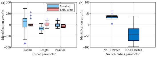
Figure 6.
Identification errors of track parameter. (a) Curve-line section. (b) Switch section.
According to the Code for Design of High-Speed Railway, for a design speed of 350 km/h, the maximum radius of mainline horizontal curves is 12,000 m, with a minimum typical radius of 7000 m and a minimum exceptional radius of 5500 m under constrained conditions. The radius values within the range of 6000 m to 12,000 m are typically incremented in intervals of 1000 m. As shown in Figure 6a, the identification error of the mainline curve radius is less than 500 m. Therefore, the curve radii specified in the Code for Design of High-Speed Railways are taken as the interval centers, with a set interval range of 500 m; the identified curve parameters falling within each interval can be replaced by the midpoint value of that interval to obtain an accurate curve radius.
Figure 6b shows the identification errors of track parameter identification in the switch section. It can be seen that the maximum identification errors for the lead curve radius of No. 12 and No. 18 switches (350 m and 1000 m, respectively) are only 61.2 m and 97.6 m. Therefore, the switch type can be determined based on the identified transition curve radius.
4. Dynamic Response Characteristics of Transverse Load
This study takes the load-time history in the upward direction as the research object, and the time-domain and frequency-domain characteristics of the transverse load are analyzed. At this time, Axle 2 refers to the front axle in the train operating direction.
4.1. Curve-Line Operating Condition
Figure 7 presents the time-domain signals of speed, gyroscope, and transverse load as the train decelerates and sequentially passes through a right-hand curve-line section and a left-hand curve-line section. According to the curve identification results, both the right-hand curve and left-hand curve have a radius of 9000 m, with superelevation values of 125 mm and 100 mm, respectively. It can be observed that the transverse loads on axle 1 and axle 2 of the bogie exhibit clear trend components during the curve-line section. On the right-hand curve, the difference between the two axles is minor, with trend component amplitudes around −2.4 kN. However, on the left-hand curve, significant differences in both amplitude and direction of the trend components are observed, with the trend components of the transverse loads on axle 1 and axle 2 being approximately 10 kN and −3.5 kN, respectively. Additionally, due to varying train speeds while passing over the curves, noticeable differences in transverse loads are observed on the same axle. These results indicate that transverse loads on curve-line sections are closely related to track geometry parameters and operating conditions.
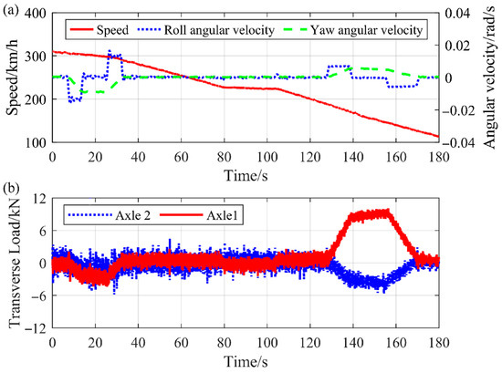
Figure 7.
Time-domain signal under curve-line section. (a) Time-domain signals of speed and gyroscope. (b) Time-domain signals of transverse load.
4.2. Straight-Line Operating Condition
According to the train’s speed, the straight-line section can be further classified into accelerating, decelerating, and constant-speed conditions. Figure 8 shows the time-domain signals of speed, gyroscope data, and transverse loads under an accelerating straight-line condition. It can be observed that the transverse loads on axle 1 and axle 2 exhibit no significant trend component, and the overall load amplitude is approximately proportional to the train speed. The load characteristics under decelerating straight-line conditions are similar to those of accelerating conditions and are, therefore, not further elaborated.
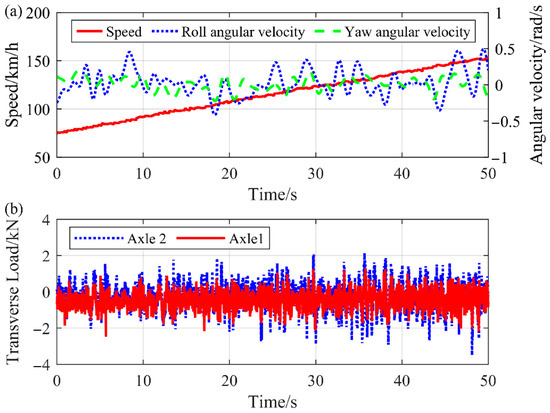
Figure 8.
Time-domain signal under accelerating straight-line section. (a) Time-domain signals of speed and gyroscope. (b) Time-domain signals of transverse load.
Figure 9 presents the time-domain signals and frequency spectra of speed, gyroscope, and transverse loads under a steady-speed straight-line section. It can be observed that the transverse loads on both the first and second axles show no significant trend component. The transverse load amplitude of the second axle is significantly greater than that of the first axle. Both axles share the same dominant frequencies at 4.7 Hz and 33.8 Hz, corresponding to the hunting motion frequency and the wheel rotation frequency, respectively. Across all frequency bands, the transverse load amplitude of the second axle is higher than that of the first, especially near the hunting motion frequency, indicating more intense lateral movement of the leading axle in the train’s operating direction.
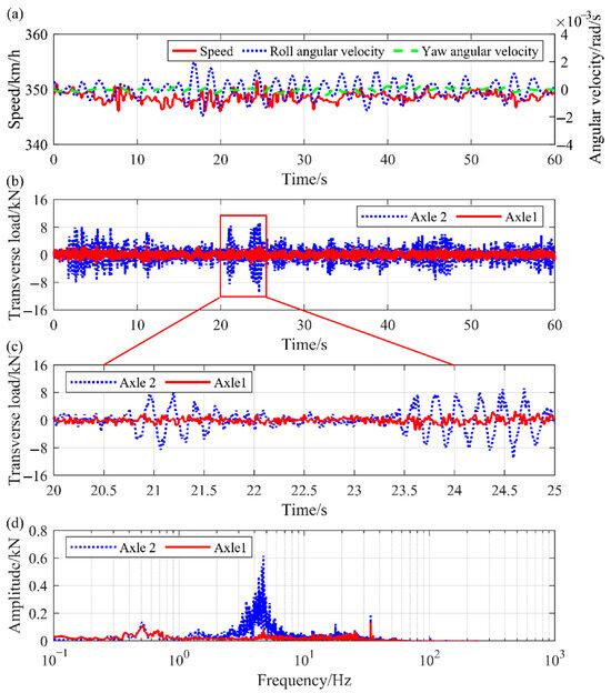
Figure 9.
Time-domain signal and spectrum under constant-speed straight-line condition. (a) Time-domain signals. (b) Frequency spectra. (c,d) gyroscope, and transverse loads under a steady-speed straight-line section.
The theoretical wheel-rotation fundamental is calculated by Equation (2). The tested wheels were measured before the test. The effective rolling diameter was Deff = 920 mm. At the running speed of 350 km/h (97.22 m/s) and with an effective wheel rolling diameter of 920 mm, the theoretical wheel-rotation fundamental frequency can be calculated as 33.6 Hz. The measured spectrum exhibits a dominant peak at 33.8 Hz, which agrees very well with the theoretical prediction (relative error ≈ 0.6%). In addition, a strong component at 4.7 Hz is observed, corresponding to the hunting motion frequency, which falls within the expected range predicted by the lateral dynamics model. These results demonstrate the consistency between theoretical and measured peaks.
4.3. Switch Operating Condition
Figure 10 shows the time-domain signals of speed, gyroscope, and transverse load during the diverging movement of a No. 18 switch in the station approach phase. It can be seen that the train passes over the small-radius lead curve of the switch at a low speed, with the transverse load characterized by a low-frequency trend component. Due to intensified wheel–rail interaction on the small-radius lead curve, the transverse load exhibits sharp fluctuations, with the peaks of transverse load on axle 1 and axle 2 reaching 12.1 kN and 12.2 kN, respectively.
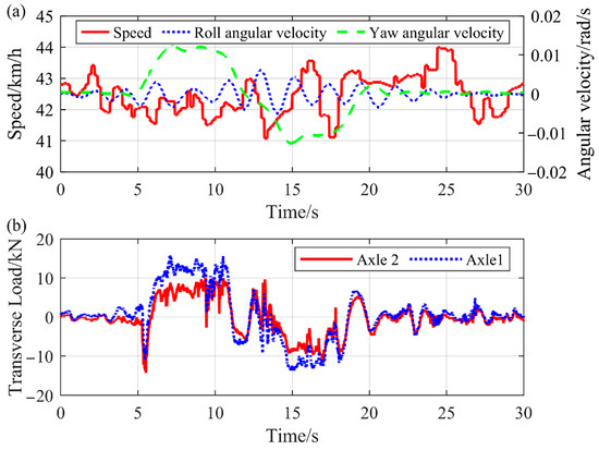
Figure 10.
Time-domain signals during diverging movement in station approach phase. (a) Time-domain signals of speed and gyroscope. (b) Time-domain signals of transverse load.
Figure 11 presents the time-domain signals of speed, gyroscope, and transverse load during the straight movement of the switch section in station departure. Since the train does not pass through a small-radius lead curve in the straight movement section, the transverse load shows no apparent trend component and fluctuates around zero. Due to the complex track geometry within the switch section and the relatively low train speed, the transverse load is characterized by low-frequency, high-amplitude fluctuation. The transverse load amplitudes on axle 1 and axle 2 show a high degree of consistency, with peak values of 3.8 kN and 5.0 kN, respectively.
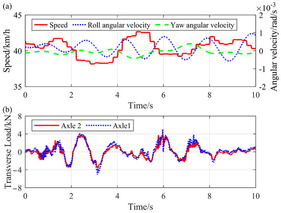
Figure 11.
Straight movement of the switch section at departure station. (a) Time-domain signals of speed and gyroscope. (b) Time-domain signals of transverse load.
5. Statistical Characteristics of Transverse Load
5.1. Different Track Conditions
To comprehensively reflect the amplitude fluctuations of the transverse load, the root mean square (RMS) values of the transverse load under different track conditions were calculated and statistically analyzed, as shown in Figure 12. Among them, the transverse load samples for mainline straight-line sections and curve-line sections were selected based on the actual operating speed level (310 km/h). For the curve-line sections, the RMS values were calculated after removing the trend component to eliminate its influence. The selected load samples correspond to axle 2, which is the leading axle in the direction of operation.
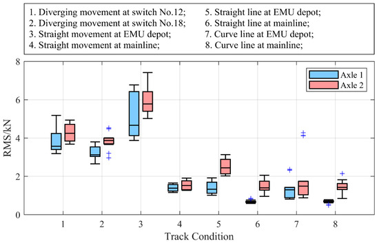
Figure 12.
RMS value of transverse load under different track conditions.
In the switch sections, the transverse load differences between axle 1 and axle 2 are relatively small. Both the diverging movement and the straight movement at the EMU depot exhibit overall higher RMS levels, indicating more intense amplitude fluctuations of the transverse load in these track sections, which is consistent with the time-domain analysis results.
The average RMS value for the diverging movement of No. 12 switch is slightly higher than that of the No. 18 switch, suggesting a certain correlation between the amplitude fluctuations of the transverse load and the switch type. The RMS values of transverse loads in the straight movement at the EMU depot are significantly higher than those in the straight movement at the mainline section, possibly due to the complex switch layout and more severe track conditions in the EMU depot areas.
In straight-line sections, the RMS values of transverse loads on bogie axle 1 and axle 2 show a clear difference, with axle 2 exhibiting significantly higher RMS levels than axle 1, indicating that the transverse load on the bogie is related to the train’s direction of operation. In the straight section within the EMU depot, although the train operates at a relatively low speed, both axles display relatively high RMS levels, which may be attributed to the severe track conditions in these sections.
In curve-line sections, the overall RMS levels of transverse loads on axle 1 and axle 2 are comparable to those in straight-line sections at the same speed level. Similarly, a significant difference exists between the RMS levels of axle 1 and axle 2.
The above results indicate that the amplitude of transverse loads is closely related to the track conditions, with significant fluctuations observed in switch and depot sections. Meanwhile, when developing the transverse load spectrum, load samples from both operating directions of the train should be selected in a balanced manner to fully capture the bogie’s loading characteristics.
5.2. Different Speed Level
Figure 13 shows the fitted curves of trend component amplitudes of transverse load versus train speed for axle 1 and axle 2 on a 9000 m radius curve with 100 mm superelevation. The corresponding fitting coefficients (a, b, and c, representing the quadratic, linear, and constant terms, respectively) are listed in Table 1. The coefficient of determination R2, which measures the goodness of fit, is close to 1, indicating a quadratic nonlinear relationship between the amplitude of the trend component and train speed. The fitted curves show that the critical speeds vz, at which the amplitude of the trend component becomes zero, are nearly equal for left- and right-hand curves on the same axle. Specifically, for axle 1, the critical speeds are 301.4 km/h and 306.9 km/h, while for axle 2, they are 238.8 km/h and 245.0 km/h. This suggests that the amplitudes of the trend component exhibit approximate symmetry around zero for each axle. As train speed increases, the trend component amplitudes of transverse loads on both axles decrease initially, then increase in the opposite direction.
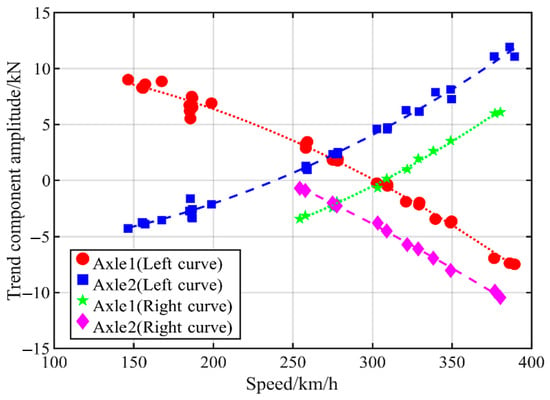
Figure 13.
Fitted curves of trend component amplitudes of transverse load versus train speed.

Table 1.
Fitting coefficients of trend component amplitudes of transverse load versus train speed.
Figure 14 shows the RMS values of transverse loads on both axles in straight-line sections and curve-line sections at different speed levels, where the values for curve-line sections are calculated after removing the trend component. It can be observed that the RMS values for both axles generally increase proportionally with operating speed, indicating intensified relative lateral motion between the wheelsets and the bogie as speed increases. The significant difference in RMS values of transverse load between axle 1 and axle 2 is consistent with the previous analysis.
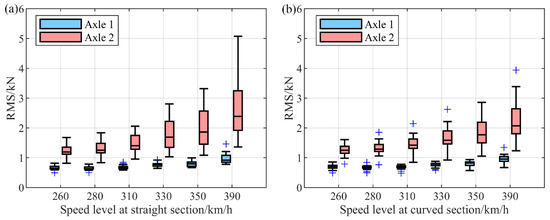
Figure 14.
RMS values of transverse loads at different speed levels. (a) RMS values of transverse loads on both axles in straight-line section. (b) RMS values of transverse loads on both axles in curve-line sections.
5.3. Different Curve Superelevation
To balance the inertial centrifugal force generated when the train negotiates curves and to ensure passenger comfort, a proper superelevation must be provided on the curve. This is typically achieved by keeping the inner rail level unchanged and raising the outer rail elevation.
According to the force balance relationship of the train negotiating a curve, the relationship between the curve superelevation h, the operating speed v, and the curve radius R is given by Equation (3) [33]:
To accommodate varying requirements for superelevation due to differences in train speed and traction mass, the design superelevation of curves is determined based on the root mean square speed vp [34]. When v = vp, the required superelevation to balance the centrifugal force equals the actual superelevation, resulting in equal load on both inner and outer rails. When v > vp, the required superelevation exceeds the actual value, leading to deficient superelevation, where the outer rail bears an unbalanced load. The direction of the bogie’s transverse load is directed from the outer rail to the inner rail. Conversely, when v < vp, the required superelevation is less than the actual value, resulting in excessive superelevation, with the inner rail bearing an unbalanced load. The direction of the transverse load acting on the bogie frame is directed from the inner rail to the outer rail.
Figure 15 shows the fitted curves between the trend component amplitudes of the transverse load and train speed under different superelevation values (right-hand curve, r = 10,000 m). The corresponding fitting coefficients are listed in Table 2. It can be observed that the coefficient of determination R2 is close to 1 in all cases, indicating that the quadratic nonlinear relationship between train speed and the trend component amplitude of transverse load remains valid under different superelevation conditions. The critical speed ve is proportional to the superelevation value at which the transverse loads on axle 1 and axle 2 are equal. At this speed, the trend component amplitude is negative, which, based on load calibration results, implies that the outer rail bears more load. Accordingly, the direction of the transverse load on both axles is from the outer rail to the inner rail, corresponding to a deficient superelevation condition. Taking the transverse load on axle 2 as an example, at an operating speed of 300 km/h, the trend component amplitudes under superelevation of 95 mm, 105 mm, and 110 mm are −3.4 kN, −2.3 kN, and −1.9 kN, respectively, indicating that curve superelevation has a significant influence on the trend component of transverse load.
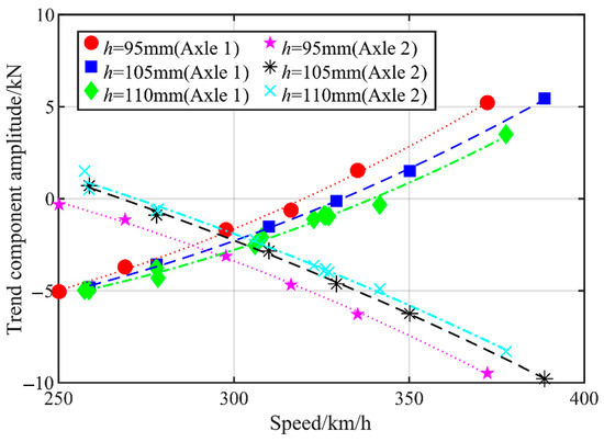
Figure 15.
Fitting curves of trend component amplitude of transverse load versus train speed under different curve superelevation.
Table 2.
Fitting coefficients of trend component amplitudes of transverse load and train speed under different curve superelevation.
5.4. Different Curve Radius
Figure 16 presents the fitted curves of the trend component amplitudes of transverse loads versus train speed under right-turn curves with different radius (superelevation h = 100 mm). The corresponding fitting coefficients are listed in Table 3. The coefficient of determination R2 is close to 1 in all cases, indicating that a quadratic nonlinear relationship remains valid between speed and the trend component amplitudes of transverse loads for different radius curves. Similar to the influence of superelevation, the critical speed ve is proportional to the curve radius. At ve, the trend component amplitude is negative, indicating that the outer rail bears an unbalanced load. The direction of transverse loads on both axles is from the outer rail to the inner rail, corresponding to a deficient superelevation condition.
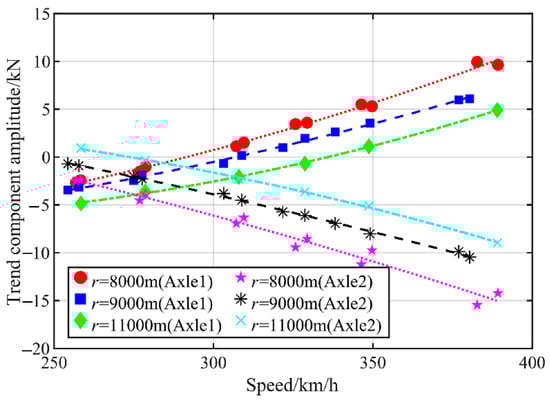
Figure 16.
Fitting curves of transverse load trend amplitude versus train speed under different curve radii.
Table 3.
Fitting coefficients of trend component amplitudes of transverse load and train speed under different curve radii.
5.5. Transverse Load Spectrum
The rain flow counting was performed on the time histories of transverse loads at each speed level to generate a 16-level transverse load spectrum. The load samples corresponding to each speed level include data from one round trip through the test section and the EMU depot entry/departure section, ensuring a comprehensive representation of the transverse load conditions at axle 1 and axle 2.
Figure 17 shows the transverse load spectrum of axle 1 and axle 2 under different speed levels. The spectrum descriptors, including the shape index (ν), spectrum length (H0), and maximum load amplitude (Smax), are listed in Table 4. It can be observed that for the same speed level, the transverse load spectrum parameters of axle 1 and axle 2 are generally consistent. This indicates that when load samples are evenly selected from both running directions, the differences in the transverse load spectrum between axle 1 and axle 2 are negligible, and the overall transverse load conditions of the bogie are similar. The load cycles of level 1 to level 10 with larger amplitudes show no clear correlation with train speed, mainly because they originate from the EMU depot entry/departure and station entry/departure sections, where the train runs under speed-limited conditions with no significant speed variation. In contrast, transverse load cycles of level 11 to level 15 mainly originate from mainline operation, where the overall load amplitude is approximately proportional to train speed. Consequently, the increase in load amplitude leads to a corresponding increase in the shape index of the load spectrum.
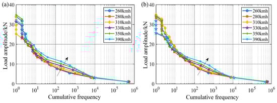
Figure 17.
Transverse load spectrum at different speed levels. (a) Front axle (b) Rear axle.
Table 4.
Parameters of transverse load spectrum at different speed levels.
6. Conclusions
This study implemented a transverse load identification method by instrumenting locating arms with strain-gauge-based bending cells, followed by as-installed bi-directional calibration under service-like lateral-stop constraints. The calibrated locating arms were subsequently applied in long-distance field tests using a CR 400BF high-speed EMU, covering multiple speed levels (260–390 km/h) and diverse line conditions. The comprehensive dataset acquired—synchronized with GPS and gyroscope signals at high sampling rates—ensured reliable load identification and provided a solid experimental foundation for analyzing transverse load characteristics and constructing representative load spectra.
This paper proposed a gyroscope-GPS-based method for identifying typical operating conditions of high-speed trains. By analyzing the time-domain characteristics of roll and yaw angular velocities and applying threshold-based logic, four representative conditions—straight lines, curves, and switch sections (straight and diverging movements)—were effectively recognized and localized. The identified mainline curve ridus showed errors within 500 m compared with track maintenance data, while the switch recognition accuracy also satisfied design specifications, demonstrating the reliability and stability of the method. Compared with existing approaches that rely on complex signal processing, the proposed method is straightforward, parameter-efficient, and well-suited for rapid recognition and synchronization of large-scale datasets. This provides a solid basis for the subsequent analysis of transverse load characteristics and the construction of load spectra.
By analyzing the time- and frequency-domain characteristics of transverse loads, the following conclusions can be summarized: under curve conditions, the transverse loads exhibit a distinct trend component, whose magnitude and direction are closely related to curve radius, superelevation, and operating speed, with noticeable differences between the two axles; in straight-line acceleration conditions, the trend component is weak, and the overall load amplitude increases approximately proportionally with speed; in constant-speed straight-line conditions, both axles show no obvious trend component; however, clear dominant frequencies appear at the hunting motion frequency (≈4.7 Hz) and the wheel rotation frequency (≈33.8 Hz), which agree well with theoretical values; moreover, the leading axle in the running direction exhibits more intense lateral motion; in switch sections, diverging movement through small-radius lead curves produces a low-frequency trend component accompanied by strong fluctuations, with peak loads exceeding 12 kN, whereas straight movement through switches shows no significant trend component and is dominated by low-frequency, large-amplitude fluctuations, with similar amplitudes on both axles (≈3.8–5.0 kN). Overall, these results indicate that transverse loads under curve and switch conditions are most significantly influenced by track geometry and wheel–rail interactions, while straight-line conditions better reflect the intrinsic dynamic characteristics of the vehicle.
The statistical analysis of transverse loads under various conditions reveals several consistent patterns. Under different track conditions, RMS values of transverse loads are significantly higher in switches and depot sections compared with mainline straights and curves, indicating stronger amplitude fluctuations. In straight-line sections, notable differences exist between axles, with the leading axle exhibiting more intense lateral motion. Under different speed levels, when the train operates on curves, the amplitude of the transverse load trend component exhibits a quadratic nonlinear dependence on operating speed. The critical speeds, defined as the points where the fitted trend-component amplitude becomes zero, are approximately the same for left-hand and right-hand curves on the same axle. In both curve and straight-line conditions, the RMS values of transverse loads on the two axles increase proportionally with train speed, with axle 2 consistently exhibiting higher levels than axle 1. Under different curve superelevation, the quadratic nonlinear relationship between train speed and the amplitude of the transverse-load trend component remains valid. The critical speed ve, at which the transverse loads on axles 1 and 2 become equal, is proportional to the magnitude of the superelevation. At this speed, the trend component of transverse loads is negative, indicating that the outer rail bears more load, corresponding to a deficient superelevation condition. Under different curve radius, the quadratic nonlinear relationship between train speed and the amplitude of the transverse-load trend component remains valid. Similar to the influence of superelevation, the critical speed ve is proportional to the curve radius. At this speed, the trend component amplitude becomes negative, indicating that the outer rail bears an unbalanced load and that the transverse load direction is from the outer rail to the inner rail, corresponding to a deficient superelevation condition.
A 16-level rain flow-based transverse load spectrum was constructed using data from both mainline and depot operations. The results show that axle-1 and axle-2 spectra are generally consistent, indicating comparable loading states. Small-amplitude cycles mainly originate from depot and station segments and show little dependence on speed, while large-amplitude cycles primarily arise from mainline operation and scale with train speed, leading to an increase in the spectrum shape index.
These findings enable standard localization and design optimization for bogie frames in region-specific environments. First, the speed-dependent quadratic law and the ve (superelevation h, curve radius r) relation allow engineers to predict trend loads under planned line upgrades (e.g., changes in speed policy, superelevation, or curve radius), supporting what-if evaluations of fatigue hot spots. Second, the rain flow-based transverse load spectra per speed level can be used directly in fatigue strength checks and accelerated test profiles, reducing over-conservatism relative to generic standards. Third, the demonstrated directional equivalence (with balanced sampling) justifies data aggregation strategies and test-time reduction without sacrificing statistical validity. Fourth, the identification that switch and depot segments dominate large-amplitude cycles provides a maintenance prioritization lever (e.g., geometry quality at switches, EMU depot track maintenance) with measurable impact on load cycles. Finally, the locating arm sensing and bi-directional calibration offer a repeatable blueprint for future development, enabling continuous health monitoring and feedback into lightweight design decisions.
Author Contributions
C.J., writing—review and editing; Y.G., writing—original draft, formal analysis, visualization; Z.L., methodology, conceptualization; G.Y., methodology, supervision. All authors have read and agreed to the published version of the manuscript.
Funding
This work was supported by National Natural Science Foundation of China (Grant No. U2468210, 52172397) and Fund Project of China Academy of Railway Sciences Group Co., Ltd. (Grant No. 2024YJ082).
Data Availability Statement
The original contributions presented in this study are included in the article. Further inquiries can be directed to the corresponding author.
Conflicts of Interest
The authors declare that they have no known competing financial interests or personal relationships that could have appeared to influence the work reported in this paper.
References
- EN 13749:2011(E); Railway Applications—Wheelsets and Bogies—Method of Specifying the Structural Requirements of Bogie Frames. European Committee for Standardization: Brussels, Belgium, 2011; pp. 19–50.
- UIC 615-4; Tractive Units Bogies and Running Gear Bogie Frame Structure Strength Tests. International Union of Railways: Paris, France, 2003; pp. 2–12.
- JIS E 4207:2004(E); Truck Frames for Railway Rolling Stock-General Rules for Design. Japanese Standards Association: Tokyo, Japan, 2004; pp. 4–5.
- Wang, B.; Li, Q.; Ren, Z.; Sun, S. Improving the fatigue reliability of metro vehicle bogie frame based on load spectrum. Int. J. Fatigue 2020, 132, 105389. [Google Scholar] [CrossRef]
- Ji, C.; Sun, S.; Li, Q.; Ren, Z.; Yang, G. Realistic fatigue damage assessment of a high-speed train bogie frame by damage consistency load spectra based on measured field load. Measurement 2020, 166, 108164. [Google Scholar] [CrossRef]
- Wang, B.; Sun, S.; Li, Q.; Tang, Q. Research on the Improvement of Speed Increased Passenger Car Bogie Frame Reliablility Based on Load Spectrum. J. China Railw. Soc. 2019, 41, 23–30. [Google Scholar] [CrossRef]
- Ma, X. Research on Some Issues of Dynamic Load Location Identification in Time Domain. Master’s Thesis, Nanjing University of Aeronautics and Astronautics, Nanjing, China, 2012. [Google Scholar]
- Ren, Z.; Sun, S.; Li, Q.; Liu, Z. Experimental studies of load characteristics of bogie frames for 350 km/h EMUs. Proc. Inst. Mech. Eng. Part F J. Rail Rapid Transit 2012, 226, 216–227. [Google Scholar] [CrossRef]
- Ren, Z.; Cao, J.; Li, Y.; Wang, B.; Wei, X. The load characteristics of the bogieframe of high-speed EMU. Eng. Mech. 2021, 38, 242–256. [Google Scholar]
- Ren, Z.; Zhao, Y.; Li, Y.; Wang, B.; Wang, Y. Loads and Damage Characteristics of the Traction and Brake Devices of Bogie of High Speed EMU. J. Mech. Eng. 2022, 58, 151–158. [Google Scholar]
- Ren, Z.; Sun, S.; Li, Q. Axle Spring Load Test and Dynamic Characteristics Analysis of High Speed EMU. J. Mech. Eng. 2010, 46, 109–115. [Google Scholar] [CrossRef]
- Zhang, Y.; Sun, S.; Yang, G.; Li, G. Load Characteristics and Fatigue Damage Assessment of High Speed Train Bogie Frame. J. Mech. Eng. 2020, 56, 163–171. [Google Scholar]
- Ji, C.; Sun, S.; Yang, G.; Meng, Q. Study on Torsional Load Characteristics of High-speed Train Bogie Frame. J. Mech. Eng. 2021, 57, 147–157. [Google Scholar]
- Gao, Y. Study on Load Characteristics of Bogie Frame in Alpine EMU. Master’s Thesis, Beijing Jiaotong University, Beijing, China, 2017. [Google Scholar]
- Wu, Y.; Ren, Z. Fatigue Damage Assessment of a Metro Vehicle Bogie Frame Based on Measured Field Load. Machines 2025, 13, 306. [Google Scholar] [CrossRef]
- Li, J.; Ren, Z.; Wu, Y.; Rui, A. Fatigue damage assessment of high-speed train bogie frame load spectra based on phase reconstruction. Eng. Fail. Anal. 2024, 159, 108008. [Google Scholar] [CrossRef]
- Zhang, Z.; Wu, X.; Zheng, Y.; Liu, Y.; Jin, X.; Zhou, J.; Chi, M.; Wen, Z. Study on vibration fatigue of lifeguard in a metro bogie and methodology for damage estimation based on the measured acceleration. J. Vib. Control 2024. [Google Scholar] [CrossRef]
- Wu, X.; Gao, A.; Wen, Z.; Wu, S.; He, S.; Chi, M.; Liang, S. Online estimation of fatigue damage of railway bogie frame based on axle box accelerations. Veh. Syst. Dyn. 2023, 61, 286–308. [Google Scholar] [CrossRef]
- Tao, G.; Liu, Z.; Ji, C.; Yang, G. Establishment and Analysis of Load Spectrum for Bogie Frame of High-Speed Train at 400 km/h Speed Level. Machines 2024, 12, 382. [Google Scholar] [CrossRef]
- Zhang, Z. Study on Load Spectrum of 400 km/h EMU Bogie Frame. Master’s Thesis, Beijing Jiaotong University, Beijing, China, 2018. [Google Scholar]
- Su, F. Research on Load and Dynamic Stress Tracking Period of Bogie Frame of High-Speed EMU. Master’s Thesis, Beijing Jiaotong University, Beijing, China, 2023. [Google Scholar] [CrossRef]
- Qiao, S. Research on High-Speed Train Working Condition Recognition Based on Multi-Scale Entropy of Frame Load Signal. Master’s Thesis, Beijing Jiaotong University, Beijing, China, 2021. [Google Scholar]
- Zhang, Y. Study on Fatigue Damage of High-Speed EMU Frame Based on Working Condition Identify. Ph.D. Thesis, Beijing Jiaotong University, Beijing, China, 2019. [Google Scholar]
- Chen, D.; Sun, S.; Li, Q.; Lin, F.; Xiao, Q. Development of the Railway Working Condition Recognition Software. J. Mech. Eng. 2019, 55, 176–184. [Google Scholar]
- Chen, D. Study on Establishment of Standardized Load Spectrum on Bogie Frames of High-Speed Trains. Ph.D. Thesis, Beijing Jiaotong University, Beijing, China, 2018. [Google Scholar]
- Rao, Q. Research on Condition Recognition of High Speed Train Bogie Based on Multi-View Clustering Ensemble. Master’s Thesis, Southwest Jiaotong University, Chengdu, China, 2018. [Google Scholar]
- Guo, C. Research on Condition Recognition of High Speed Train Based on Deep Learing and Classification Ensemble. Master’s Thesis, Southwest Jiaotong University, Chengdu, China, 2017. [Google Scholar]
- Zou, H. Load Spectrum Study on Intercity EMU Bogie Frame. Ph.D. Thesis, Beijing Jiaotong University, Beijing, China, 2016. [Google Scholar]
- Wang, M. Study on Characteristics and Applications of On-track Load of Welded Bogie Frame. Ph.D. Thesis, Beijing Jiaotong University, Beijing, China, 2016. [Google Scholar]
- Hou, J.; Yi, Y. Design of railway transition curve. Theor. Res. 2012, 10, 27–28. [Google Scholar]
- Bao, K. Simulation Study on Dynamic Performance of Transition Curve Parameters of High-Speed Railway. Master’s Thesis, Southwest Jiaotong University, Chengdu, China, 2012. [Google Scholar]
- TB 10621-2014; Code for Design of High Speed Railway. National Railway Administration of the People’s Republic of China: Beijing, China, 2014; pp. 17–22.
- Sun, L.; Cui, S.; Yan, Z.; Liang, C.; Yu, H. Study on Adaptability of Curve Superelevation with Speed of Beijing-Shanghai High Speed Railway Being Increased to 400 km/h. J. China Railw. Soc. 2021, 61, 96–99. [Google Scholar]
- Hu, H. Study on the Allowable Cant Deficiency Value for the Curve Section of High Speed Railway. China Railw. 2019, 32–40. [Google Scholar]


Disclaimer/Publisher’s Note: The statements, opinions and data contained in all publications are solely those of the individual author(s) and contributor(s) and not of MDPI and/or the editor(s). MDPI and/or the editor(s) disclaim responsibility for any injury to people or property resulting from any ideas, methods, instructions or products referred to in the content. |
© 2025 by the authors. Licensee MDPI, Basel, Switzerland. This article is an open access article distributed under the terms and conditions of the Creative Commons Attribution (CC BY) license (https://creativecommons.org/licenses/by/4.0/).