Abstract
In many real-world control tasks, agents operate under partial observability, where access to complete state information is limited or corrupted by noise. This poses significant challenges for reinforcement learning algorithms, as methods relying on full states or long observation histories can be computationally expensive and less robust. Four-Phase Rapid Motor Adaptation (FRMA) is a reinforcement learning framework designed to address these challenges in high-frequency control tasks under partial observability. FRMA proceeds through four sequential stages: (i) full-state pretraining to establish a strong initial policy, (ii) auxiliary hidden-state prediction for LSTM memory initialization, (iii) aligned latent representation learning to bridge partial observations with full-state dynamics, and (iv) latent-state policy fine-tuning for robust deployment. Notably, FRMA leverages full-state information () only during training to supervise latent representation learning, while at deployment it requires only short sequences of recent observations and actions. This allows agents to infer compact and informative latent states, achieving performance comparable to policies with full-state access. Extensive experiments on continuous control benchmarks show that FRMA attains near-optimal performance even with minimal observation–action histories, reducing reliance on long-term memory and computational resources. Moreover, FRMA demonstrates strong robustness to observation noise, maintaining high control accuracy under substantial sensory corruption. These results indicate that FRMA provides an effective and generalizable solution for partially observable control tasks, enabling efficient and reliable agent operation when full state information is unavailable or noisy.
1. Introduction
Reinforcement learning (RL) is a computational framework in which agents learn to make decisions by interacting with an environment and receiving feedback in the form of rewards [1,2]. Unlike supervised learning, RL does not require labeled datasets; instead, agents discover optimal behavior through direct exploration. This makes RL highly suitable for sequential decision-making problems where explicit models are unavailable or inaccurate.
Over the past decade, RL has achieved significant milestones in domains such as game playing [3], robotic control [4,5], and continuous control environments like MuJoCo [6,7]. These successes are largely attributed to the ability of RL algorithms to learn policies in high-dimensional, nonlinear environments directly from experience. However, many real-world or physics-based simulated environments are only partially observable—the agent does not have direct access to the full system state and must instead infer latent dynamics from limited observations, which may be noisy or partially missing.
Such settings are commonly modeled as Partially Observable Markov Decision Processes (POMDPs) [8,9], which introduce additional complexity to the learning problem. In POMDPs, the agent does not have direct access to the full environment state; instead, it must infer latent states from partial observations. To make informed decisions, agents typically maintain a memory of past observations and actions, which is especially important in environments with long-term dependencies or delayed rewards.
To address partial observability, the Rapid Motor Adaptation (RMA) framework [10] has been proposed. RMA operates in two stages: first, it learns a base policy with full-state access ; second, it trains an encoder to approximate a latent state representation from sequences of past observations and actions . This allows the policy to be deployed under partial observability as , leveraging historical information to infer hidden states.
While RMA has demonstrated strong performance in low-frequency robotic locomotion tasks, its reliance on fixed-length input windows and infrequent inference steps limits its applicability in high-speed control tasks or environments with rapidly changing latent dynamics.
To overcome these challenges, this paper proposes a general framework called Four-Phase Rapid Motor Adaptation (FRMA). FRMA extends the RMA design with a four-phase training pipeline, enabling high-frequency decision-making under partial observability. The four phases are designed to progressively transfer knowledge from full-state information to compact latent representations that can be used for robust control with only partial observations:
- Full-State Pretraining: A base policy is first trained using full access to the ground-truth system state. This policy captures essential control behaviors without concern for observability constraints, providing a strong performance ceiling and serving as a foundation for subsequent learning stages.
- Auxiliary Hidden-State Prediction: An auxiliary network is trained to predict the initial hidden and cell states of the recurrent encoder (LSTM) from recent observation–action sequences. These predicted states initialize the LSTM memory, enabling immediate inference of latent dynamics, even in partially observable conditions.
- Aligned Latent Representation Learning: A recurrent encoder is trained to map sequences of partial observations and actions to latent states that are aligned with those learned during full-state training. This phase bridges the gap between limited observations and the underlying full latent states, ensuring that the encoder produces informative representations for policy execution.
- Latent-State Policy Fine-Tuning: Finally, the policy is fine-tuned using only the estimated latent encoding , allowing it to operate under realistic partially observable conditions. This phase ensures that the agent can perform fast, reliable control without requiring full-state information at deployment.
FRMA introduces several core innovations that make it particularly suitable for high-frequency, partially observable control tasks:
- High-Frequency, Single-Step Adaptation: During training, FRMA leverages multi-step sequence regression to learn latent-state inference. At deployment, it switches to single-step LSTM updates, continuously updating the hidden and cell states at each timestep. This allows the latent encoding to be refreshed at high frequency, enabling rapid and precise control.
- Extended Temporal Coverage: By propagating the LSTM’s hidden and cell states across timesteps, FRMA avoids fixed-horizon limitations (e.g., 50-step windows). It effectively captures long-term temporal dependencies without the computational burden of long input sequences, reducing GPU memory usage and accelerating both training and inference.
- Policy-Invariant Latent Representation: Observation–action histories contain both environmental dynamics and policy-dependent information. FRMA uses supervised learning to ensure that the LSTM hidden and cell states primarily encode environment dynamics, effectively minimizing the influence of the sampling policy . This design enhances generalization and robustness when the policy changes or under different deployment conditions.
The remainder of this paper is organized as follows. Section 2 reviews related work on recurrent neural networks, reinforcement learning, and the RMA framework, providing the technical background for FRMA. Section 3 presents the FRMA framework in detail, describing each of the four sequential stages. Section 4 details the experimental setup and results, demonstrating FRMA’s performance on continuous control tasks in the MuJoCo environment. Finally, Section 5 concludes the paper and discusses potential avenues for extending the FRMA framework.
2. Related Work
2.1. Artificial Neural Networks
Artificial neural networks (ANNs) have achieved remarkable success across a wide range of machine learning tasks [11,12]. Feedforward neural networks (FNNs), such as multilayer perceptrons, can approximate arbitrary functions given sufficient data and model capacity, and are commonly applied to static input–output mappings [13]. However, in dynamic environments where temporal dependencies are critical, FNNs are limited by their inability to retain historical context. Recurrent neural networks (RNNs) and their variants, such as long short-term memory (LSTM) networks [14,15,16], address this limitation by incorporating memory through recurrent connections. This allows information to persist over time, enabling the modeling of temporal dependencies essential for tasks such as speech recognition, language modeling, and time-series prediction [17,18]. Despite these advances, traditional neural networks—including LSTM-based architectures—are typically trained in a supervised learning setting, where each input x is paired with a target output y. While effective when labeled data is abundant and the input–output mapping is relatively static, supervised learning alone struggles in complex, high-dimensional control tasks. In particular, continuous control environments with partial observability and delayed rewards—common in robotics and embodied AI—require sequential decision-making over time, which exceeds the capabilities of standard supervised approaches.
2.2. Classical Control Methods
Classical control methods have been widely applied to complex systems, including Active Disturbance Rejection Control (ADRC) [19], multilayer neurocontrol for high-order uncertain nonlinear systems [20], Robust Integral of the Sign of the Error (RISE) [21], observer-based RISE controllers [22], adaptive ADRC with recursive parameter estimation [23], and Auxiliary RISE (ARISE) controllers for nonsmooth switched systems [24]. These methods have demonstrated strong robustness and effective disturbance rejection across various engineered systems. However, classical controllers typically require accurate system modeling, and their performance may deteriorate in high-dimensional, partially observable, or stochastic environments. In contrast, neural network-based reinforcement learning approaches can learn control policies directly from data, enabling adaptive behavior in complex scenarios and offering greater flexibility and potential performance in modern control tasks.
2.3. Reinforcement Learning
Classical reinforcement learning (RL) methods can be broadly categorized into three types: tabular methods, value-based methods, and policy gradient methods. Tabular approaches, such as Q-learning and SARSA [25], maintain a lookup table estimating action values for each discrete state–action pair. While effective in low-dimensional environments, tabular methods become infeasible in continuous or high-dimensional spaces due to the curse of dimensionality. Value-based methods address this limitation by approximating the value function with neural networks, enabling generalization across large or continuous state spaces. Deep Q-Networks (DQN) [26] achieved notable success in discrete-action tasks, such as Atari games, but exhibit instability and overestimation bias in continuous domains. Policy gradient methods directly optimize parameterized policies, supporting stochastic and continuous actions. Representative examples include REINFORCE [27], Proximal Policy Optimization (PPO) [28], and Soft Actor-Critic (SAC) [29], which combines policy gradients with entropy regularization and an actor–critic architecture. Despite their success, these algorithms typically assume full observability of the environment state . In practice, many control tasks provide only partial observations , causing performance degradation when the agent cannot access complete state information. This motivates the integration of architectures capable of temporal memory and latent state inference, such as recurrent networks or encoder–decoder models, to handle partially observable environments effectively.
2.4. Observation–Action Sequence-Based Reinforcement Learning
Many reinforcement learning methods for partially observable environments rely on short histories of observations and actions to infer latent states. Rapid Motor Adaptation (RMA) and its variants are representative examples of such observation–action (oa) sequence-based RL approaches. The original RMA framework first trains a base policy using full-state trajectories and then employs a supervised adaptation module to infer a latent context from recent observation–action sequences . However, RMA is constrained by a fixed input window (typically 50 steps) and a low adaptation frequency on the order of 10 Hz [10]. Extensions of RMA address specific limitations. A-RMA explicitly fine-tunes the base policy with an imperfect extrinsic estimator to improve performance in biped locomotion, but it retains the same adaptation module and fixed-horizon inference [30]. RMA2 targets manipulation tasks by combining depth perception and symbolic embeddings to estimate latent object parameters, yet it still operates over a fixed-length OA segment and lacks high-frequency adaptation [31]. Other sequence-based RL approaches include Deep Recurrent Q-Networks (DRQN) and Action-Conditional DRQN (ADRQN), which incorporate recurrent layers over observations or observation–action streams to implicitly encode belief states, trained end-to-end via Q-learning [32,33]. Recurrent Predictive State Policy (RPSP) networks similarly learn a predictive latent belief state using supervised prediction alongside policy gradients [34]. While these methods demonstrate the utility of sequence-based encoding, they generally train the encoder jointly with the policy and maintain memory only over a truncated horizon, which can limit adaptation speed and efficiency. Overall, these OA sequence-based RL methods highlight the importance of latent-state inference from recent history, but they also reveal limitations in adaptation frequency, memory length, and policy–encoder decoupling—challenges that FRMA aims to overcome.
3. FRMA Details
This section introduces the FRMA framework in detail, including its four-phase training strategy and the inference procedure used during deployment. Table 1 summarizes all key variables and network components, and Figure 1 illustrates the sequential workflow. Detailed proofs are provided in Appendix C and Appendix D, and comprehensive pseudocode for both training and deployment is included in Appendix A.

Table 1.
Symbol definitions and network components in FRMA.
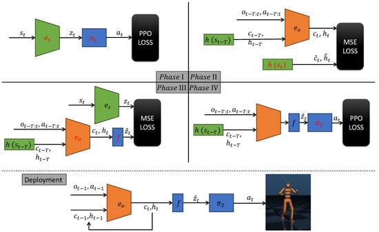
Figure 1.
Training and deployment procedure of the FRMA framework. Orange modules denote LSTM networks that extract temporal features from observation–action sequences. Blue modules correspond to multilayer perceptrons (MLPs) that map input vectors to latent encoding or actions. Green modules process full-state information; depending on the environment, these can be implemented as MLPs (e.g., in MuJoCo) or CNNs (e.g., in Atari). Black modules represent the loss functions used for optimization. In each phase, networks highlighted in red are actively trained, while networks shown in black have their parameters frozen.
The FRMA training proceeds through four sequential phases, each targeting a distinct network module and progressively bridging the gap between full-state learning and deployment under partial observability. This stagewise design ensures that FRMA can leverage full-state information during training while requiring only partial observations at deployment, achieving high-frequency adaptation, robust latent-state inference, and stable policy performance.
3.1. Phase I: Full-State Policy Learning
Phase I focuses on training the foundational policy network, , together with the state encoder, , using the complete environment state as input. This stage assumes full observability, meaning the agent has access to all relevant features of the underlying Markov Decision Process (MDP). By removing partial observability and temporal dependencies, the learning process is simplified, allowing the model to concentrate on extracting meaningful latent representations and learning basic control strategies.
The state encoder transforms the high-dimensional raw state into a compact latent vector , which serves as the input to the policy . The policy is optimized using the Proximal Policy Optimization (PPO) algorithm, which balances exploration and exploitation while ensuring stable updates via a clipped surrogate objective. In this phase, standard policy gradient methods are applied without recurrent layers or memory modules, avoiding the complexity of long-term temporal credit assignment and enabling faster convergence.
Formally, the forward pass in Phase I is expressed as:
By the end of this phase, the agent acquires a well-initialized encoder and policy capable of operating under full observability, providing a strong foundation for adaptation to partially observable environments in subsequent phases.
3.2. Phase II: Supervised Training of Hidden Network
Long short-term memory (LSTM) networks extract and integrate temporal information from observation–action sequences, encoding this knowledge in their hidden and cell states . In existing approaches, such as RMA and ARMA, this temporal integration is achieved by repeatedly processing the most recent T timesteps at each control step. While effective, such repeated sequence processing incurs significant computational cost, inherently limiting the achievable control frequency.
To address this limitation, FRMA adopts a single-step inference paradigm during deployment. Instead of recomputing over the entire T-step history at each timestep, the system maintains and incrementally updates throughout the episode. This design preserves long-term temporal information while minimizing computational latency. However, a mismatch arises between training and deployment: during training, LSTMs are typically optimized over short, fixed-length sequences, which may limit their ability to capture dependencies spanning the full episode.
To resolve this, we introduce an auxiliary hidden-state inference network , which maps the current full state directly to the corresponding . This network is trained in a supervised manner to minimize the mean squared error (MSE) between its predictions and the hidden states generated by the LSTM during full-episode rollouts. By enabling reconstruction of the LSTM’s internal memory from a single state input, this approach ensures consistency between training and deployment while retaining the computational efficiency of single-step inference.
Formally, the hidden-state inference process and training loss are defined as:
where denotes the target hidden state derived from the full state , and is the LSTM output given the partial observation–action sequence and the initialized memory at time .
This supervised training approach follows prior work on deep LSTM supervision [14,35]. Minimizing allows the LSTM to be accurately initialized at any point in an episode, enabling high-frequency control while preserving long-term temporal reasoning.
3.3. Phase III: Learning Latent Representations from Partial Observations
In realistic control settings, agents rarely have access to the full environment state , relying instead on partial and potentially noisy observations . To enable robust decision-making under such partial observability, Phase III trains the agent to reconstruct the latent representation —originally learned from full-state information in Phase I—using only past observations and executed actions. This approach follows the core principle of RMA, where a history encoder infers latent task variables from recent experience.
The LSTM-based observation encoder is initialized at the start of each sequence with hidden and cell states predicted by the hidden-state inference network from Phase II. It then processes a fixed-length window of past observations and actions to update its internal memory . These updated states are passed through a mapping network to produce the estimated latent representation . The target latent vector , computed using the state encoder trained in Phase I, serves as the ground truth.
Training minimizes the mean squared error (MSE) between and , aligning the partial-observation pathway with the full-state pathway. Through this supervised alignment, the observation encoder learns to capture temporally extended dependencies and infer task-relevant latent states without direct access to , a capability essential for real-world deployment.
Formally, the encoding and mapping process is expressed as:
By the end of this phase, the agent can reliably transform sequences of partial observations into compact latent representations that retain the task-relevant information needed for downstream policy execution.
3.4. Phase IV: Policy Fine-Tuning on Estimated Latent States
In the final phase, the control policy transitions from relying on ground-truth latent states to operating entirely on their estimated counterparts derived from partial observations. This step is essential for bridging the sim-to-real gap and ensuring robust decision-making despite reconstruction errors introduced in Phase III.
Following the ARMA-inspired design, the base policy learned in Phase I is duplicated to initialize a new policy , which is then fine-tuned using as input. This duplication preserves the well-optimized structure of while enabling to adapt its action selection to the shifted latent distribution.
Fine-tuning employs the Proximal Policy Optimization (PPO) algorithm, providing stable gradient updates under the new input distribution. The process allows the policy to compensate for systematic biases or noise in , effectively learning to act reliably using only estimated latent states. By the end of this phase, the agent achieves fully observation-based control without any dependence on privileged full-state information, completing the FRMA pipeline from full-state pretraining to deployable inference.
Formally, the fine-tuning process is expressed as:
where and are fixed from Phase III, and is optimized to maximize expected returns using as the sole input.
3.5. Training Procedure
The training of FRMA is organized into four distinct phases, each executed for a fixed number of iterations specified by the hyperparameter train_step. The second important hyperparameter, batch_size, controls the number of samples used in each parameter update. The design explicitly avoids end-to-end training from scratch; instead, each phase focuses on a targeted subset of networks to ensure stable convergence and avoid detrimental interference between modules. The procedure is as follows:
- Phase I: Full-State Policy Learning. For train_step iterations, sample batch_size state–action–reward transitions from full-state rollouts. The state encoder and the base policy are jointly optimized using Proximal Policy Optimization (PPO) under full observability. This phase establishes a high-quality latent state representation and a competent control policy, providing a strong foundation for subsequent modules.
- Phase II & III: Hidden-Network Pretraining and Joint LSTM–Mapping Training. These two phases are interleaved within each iteration to maintain a balanced learning pace between the hidden state predictor and the observation-based latent inference pipeline . For train_step iterations:
- Sample 5 independent batches to update via the hidden-state MSE loss , using full-state trajectories as supervision.
- Sample 1 fresh, non-overlapping batch to jointly optimize and by minimizing the mapping loss , which aligns the predicted latent with the ground-truth latent from Phase I.
This strict batch independence is critical: is trained on , whereas relies on . Sharing identical samples would bias toward the short-horizon regime, degrading its generalization to long-term dependencies. - Phase IV: Policy Fine-Tuning. For train_step iterations, sample batch_size trajectories of estimated latent states from the Phase III pipeline. The policy , initialized from , is fine-tuned using PPO to adapt to the noisy and potentially biased distribution of . This step completes the transition from privileged, full-state decision-making to deployable, observation-driven control.
The deliberate phase separation ensures that each module is trained under optimal supervision, minimizing interference and preventing unstable dynamics that often occur in fully joint optimization.
3.6. Deployment
After completing all four training phases, FRMA is deployed in an online control loop that operates exclusively on partial observations. The deployment strategy emphasizes high control frequency and low latency, eliminating the need to reprocess long observation–action histories at each timestep. Instead, the LSTM encoder maintains its hidden and cell states throughout the episode, updating them incrementally with each new observation-action pair.
At the start of each episode, the LSTM memory is zero-initialized:
This zero-initialization ensures fair comparison with baseline methods (ARMA, RMA, ADRQN, RPSP), which do not include a learned initializer. In principle, FRMA can reconstruct from an initial environment state using the hidden network , enabling “hot-start” inference and mitigating cold-start degradation; this feature is omitted here solely for comparability.
At each timestep t, the agent executes the following sequence:
- Receives the latest observation and executed action from the previous step.
- Updates the LSTM memory via a single forward step:
- Computes the current latent state estimate through the feature extraction network:
- Feeds into the fine-tuned policy to determine the next action:
This approach minimizes per-step computation since the LSTM state is propagated incrementally rather than recomputed from scratch. On standard hardware (Intel i9-13900K CPU or RTX 4070 GPU), the combined MLP-LSTM forward pass executes in under 1 ms per step, enabling kilohertz-range control frequencies even with batch size 1.
The deployment procedure relies on the following assumptions:
- Zero-initialization. Used here for fair comparison; FRMA inherently supports hot-start initialization via when privileged or learned initial state information is available.
- Policy optimization. Phase IV uses on-policy PPO for stability in MuJoCo, but FRMA is compatible with off-policy methods such as SAC for enhanced generalization.
- Full-state supervision during training. Ground-truth state information shapes the encoder only; deployment relies solely on partial observations. When a simulator is unavailable, FRMA can use data-driven environment models or other reconstruction methods to provide training supervision.
- Staged training. The multi-phase schedule decouples encoder learning from policy learning to improve stability and fairness; end-to-end training remains feasible within the same framework.
By aligning deployment-time inference with Phase IV fine-tuning under these assumptions, FRMA minimizes train–deploy mismatch and achieves high-frequency, low-latency control, while retaining flexibility to incorporate learned initializers, dynamic objectives, off-policy training, or alternative state reconstruction in future extensions.
4. Experiments
All experiments were conducted on a workstation equipped with an AMD EPYC 9654 96-Core Processor and an NVIDIA RTX 4090 GPU. In the figures presented below, each training curve visualizes the episode-level cumulative reward as a function of timesteps, with a maximum of 1000 timesteps per episode. Each experiment was repeated across five random seeds, and the results were averaged to ensure statistical reliability. Solid lines indicate the mean reward over sampled episodes, while shaded regions represent the variance. The full implementation, including configuration files and scripts for reproducing all figures and ablation studies, is publicly available on GitHub: https://github.com/guanyimu/FRMA.git (accessed on 20 September 2025).
The MuJoCo suite [36] provides a standard benchmark for evaluating reinforcement learning agents on continuous control tasks. Common environments such as HalfCheetah, Walker2d, and Hopper are modeled as fully observable Markov Decision Processes (MDPs), where the agent has access to the complete system state at each timestep.
To evaluate performance under partial observability, the underlying MuJoCo MDPs are converted into partially observable MDPs (POMDPs) by restricting the agent’s access to the full state. Specifically, only the first few dimensions of the state vector are retained as observations to simulate limited sensing, as summarized in Table 2. In these environments, the retained dimensions typically correspond to directly measurable quantities such as positions, distances, and angles, while the omitted dimensions include variables that are more difficult to measure, such as velocities, angular velocities, or forces. This setup reflects realistic scenarios in which some physical quantities are directly accessible, whereas others must be inferred indirectly.
Table 2.
Observation dimensionality used in each MuJoCo environment.
The following methods are evaluated in our experiments:
- FullState (baseline) [28]: A PPO agent trained with full-state access, representing an upper bound on achievable performance.
- FRMA (ours): The proposed Four-phase Rapid Motor Adaptation framework, designed for learning in partially observable environments.
- ARMA [30]: An extension of RMA that fine-tunes the base policy using full-state supervision after adaptation.
- RMA [10]: Rapid Motor Adaptation with a fixed-length encoder over recent observation–action sequences.
- ADRQN [33]: An adaptation of Deep Recurrent Q-Networks employing LSTM encoders to process partial observation–action histories.
- RPSP [34]: A recurrent predictive state policy method that explicitly models predictive latent states for control.
- TrXL [37]: A Transformer-XL-based agent using multi-head attention to encode long-term dependencies in observation–action sequences.
Since the core novelty of FRMA resides in its four-phase training procedure, the chosen baselines correspond naturally to variants of FRMA with fewer phases. Specifically, when trained in a single phase, the framework reduces to a recurrent PPO agent akin to ADRQN, directly learning from partial observation–action histories. A two-phase configuration—comprising separate encoder adaptation and policy learning—corresponds to RMA. Adding a third phase of full-state fine-tuning yields ARMA. Our full FRMA implementation completes the four-phase design. Therefore, comparisons among ADRQN, RMA, ARMA, and FRMA can be interpreted as an implicit ablation study on the number of training phases, illustrating how each successive phase contributes to stability and performance.
Detailed network architectures, including both encoder and policy designs for all methods, are provided in Appendix B to support reproducibility.
As shown in Figure 2, the FullState agent achieves the highest returns, as expected, due to access to complete environment information. Among the observation-based methods, FRMA attains performance nearly indistinguishable from FullState, maintaining comparable return values across all six environments. Furthermore, FRMA consistently outperforms RPSP, ADRQN, RMA, and ARMA in every tested scenario. Within these baselines, RPSP shows performance close to ARMA in some environments, indicating that leveraging observations rather than full states for auxiliary training can help mitigate the – mismatch. Nevertheless, state information still provides substantial guidance, so ARMA and especially FRMA ultimately achieve higher asymptotic performance.
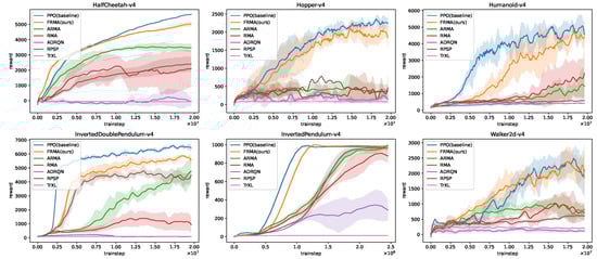
Figure 2.
FRMA training performance across the MuJoCo benchmark suite. Comparison of seven algorithms—FullState, FRMA, ARMA, RMA, ADRQN, RPSP, and TrXL—across six MuJoCo environments: InvertedPendulum, HalfCheetah, Hopper, Walker2d, InvertedDoublePendulum, and Humanoid. The FullState agent is trained with full state information and serves as an upper performance bound. All other agents rely solely on sequences of observations and actions. FRMA nearly matches FullState performance despite operating under partial observability. Each line represents the mean episode reward over five random seeds, and the shaded area indicates the reward variance.
Among the three weaker baselines, ARMA generally performs better than RMA; however, both suffer from slower convergence and lower performance ceilings. By contrast, the TrXL algorithm yields the poorest results overall. This is likely because its attention-based encoder, while capable of modeling complex, variable-length dependencies, introduces unnecessary computational overhead in the MuJoCo tasks studied here, which involve short sequences with well-defined temporal relationships. These results demonstrate that FRMA effectively reconstructs rich and informative latent representations from partial observations, enabling robust decision-making in high-dimensional continuous control tasks.
FRMA is organized as a four-phase framework, and several baseline algorithms correspond to natural stage-wise ablations of this design. Specifically, ADRQN represents the single-phase baseline that trains a recurrent policy directly from observation–action (OA) sequences without auxiliary supervision. RMA extends this by using encoder supervision derived from the simulator state encoding, i.e., the OA encoder is trained to reproduce information obtainable from . ARMA further incorporates a third phase intended to mitigate the mismatch between the initial auxiliary policy and the refined policy (policy-mismatch correction). FRMA completes the pipeline by adding a hidden-network phase that learns a mapping from the true state to the LSTM memory , thereby removing the strict dependence of the LSTM on long OA input windows.
Partially Observable Markov Decision Processes (POMDPs) require extracting informative latent state representations from histories of observation–action pairs. The key innovation of Phase II in FRMA is to model the LSTM hidden state as a function of the underlying true state , enabling supervised training that decouples the LSTM’s representational capacity from the raw number of observation timesteps. By leveraging this hidden-state network, the LSTM can encode much longer effective temporal context even when provided only a short OA segment, which reduces sensitivity to the sequence length T.
Figure 3 presents the ablation results across six MuJoCo environments, comparing FRMA and ARMA under observation–action sequence lengths . In the figure, solid lines denote FRMA and dashed lines denote ARMA. Curves of the same color correspond to the same sequence length T, allowing direct comparison between methods at each temporal window. As expected, increasing T generally improves the performance of both FRMA and ARMA, reflecting the benefit of longer sequences that provide richer temporal context. Notably, FRMA with often exceeds the performance of ARMA with , highlighting FRMA’s ability to effectively encode longer temporal dependencies even from very short observation–action segments. The marginal improvement of FRMA from to further demonstrates its low sensitivity to T, whereas ARMA continues to gain substantially from longer sequences. These results confirm that the Phase II hidden-network design allows the LSTM to maintain high representational efficiency with smaller input windows, reducing memory usage and enabling larger batch sizes without compromising performance.
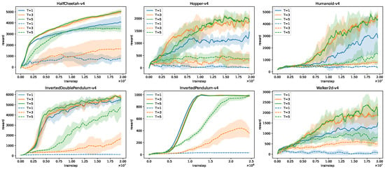
Figure 3.
Comparison of FRMA and ARMA across six MuJoCo environments under different observation–action sequence lengths . Solid lines represent FRMA, while dashed lines represent ARMA. Curves of the same color correspond to the same sequence length T. FRMA consistently outperforms ARMA, even with shorter sequences.
To further evaluate the robustness of the proposed FRMA framework in partially observable settings, Gaussian noise is added during testing either to the full state vector (for FullState) or to the partial observation vector (for all other methods). The horizontal axis represents the noise standard deviation , with larger values corresponding to stronger corruption of the input signals.
All policies are kept fixed during evaluation, so the results directly reflect the robustness of each method’s learned latent representations and decision policies under noisy inputs. For each environment and algorithm, five independent trials with different random seeds are conducted. The mean episode return is shown with solid lines, while the shaded regions indicate the standard deviation across seeds.
As shown in Figure 4, all algorithms experience performance degradation as noise levels increase, reflecting reduced fidelity of environment information. Among observation-based methods, FRMA exhibits the smallest performance drop across all environments, often approaching the robustness level of FullState. In contrast, ADRQN, RMA, and ARMA show more pronounced declines, especially at higher noise magnitudes and in high-dimensional environments such as Humanoid and HalfCheetah, where corrupted inputs can destabilize dynamics estimation in models with less temporal integration.
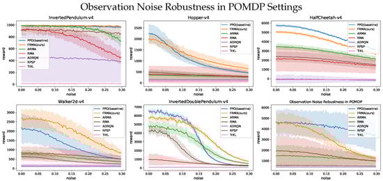
Figure 4.
Robustness evaluation under Gaussian noise for six MuJoCo environments. The horizontal axis shows the noise standard deviation , and the vertical axis shows the average episode return. Solid lines indicate mean performance across five evaluation seeds; shaded regions indicate standard deviation. Larger corresponds to stronger input corruption.
The robustness advantage of FRMA stems from its ability to reconstruct latent states over extended temporal windows and maintain LSTM memory across timesteps. This temporal integration effectively filters transient observation noise, enabling stable control despite heavy corruption of individual observations.
Additional robustness evaluations are provided in Appendix E, where five separate tables summarize the results across different perturbation scenarios:
- standard evaluation without perturbations,
- observation corrupted by Gaussian noise,
- observation dropouts with a fixed probability,
- action corrupted by Gaussian noise,
- action dropouts with a fixed probability.
Each table reports both the mean and standard deviation of episode returns for all seven algorithms (FullState, FRMA, ARMA, RMA, ADRQN, RPSP, TrXL) across six MuJoCo environments (InvertedPendulum-v4, Hopper-v4, HalfCheetah-v, Walker2d-v4, InvertedDoublePendulum-v4, Humanoid-v4).
These tables collectively demonstrate that FRMA consistently maintains higher mean returns and lower variance under all tested perturbations compared with baseline methods, confirming the framework’s superior robustness and reliability in partially observable and noisy environments. The detailed numerical results complement the qualitative trends illustrated in Figure 4 and provide a comprehensive view of performance under diverse operational conditions.
5. Conclusions and Future Work
This paper presented Four-Phase Rapid Motor Adaptation (FRMA), a modular framework that decouples latent-state inference from policy optimization to address high-frequency, partially observable control tasks. By combining supervised pretraining of a hidden-memory network with joint training of an LSTM encoder and a mapping network, FRMA enables single-step LSTM inference at deployment. This design allows the latent-state encoding to be updated at high frequency, thereby supporting rapid and robust control. Empirical results on the MuJoCo benchmark suite demonstrate that FRMA matches the performance of a full-state PPO agent while significantly outperforming existing RMA-based and recurrent policies when operating solely on observation–action histories.
Despite these promising results, several limitations and opportunities remain. First, although FRMA exhibits strong performance even with very short observation–action histories (e.g., ), indicating minimal cold-start effects, the initial hidden and cell states are currently zero-initialized. Using the hidden network to reconstruct from an initial environment state could enable hot-start initialization, further improving first-step accuracy. Second, in our experiments, the fine-tuning of is performed with on-policy PPO, exposing the LSTM encoder only to trajectories generated by this policy. If deployment encounters observation–action sequences that deviate substantially from this distribution, inference errors may exceed those of standard PPO. However, FRMA is agnostic to the choice of policy optimization algorithm; could be replaced with off-policy methods such as SAC or other policy learners to enhance generalization and robustness to out-of-distribution sequences. Third, FRMA currently relies on full-state information from a simulator to train the hidden network. While real-time simulators may not always be available due to high-frequency requirements, data-driven or learned neural-network models could serve as surrogates for , enabling FRMA training without a full simulator. Finally, FRMA currently tracks only static physical quantities or poses. Incorporating dynamic control targets as additional network inputs could enable tracking of time-varying objectives. Addressing these challenges will further enhance the robustness, versatility, and applicability of FRMA to high-frequency, safety-critical control domains.
Moreover, several recent works in power electronics and motor drives provide concrete evidence that the challenges addressed by FRMA—such as partial observability, parameter drift, nonlinear thermal–electrical dynamics, and high control rates—are active research concerns in industrial settings. For example, Dini et al. [38] demonstrates an adaptive model-predictive control scheme for six-phase synchronous motor drives that operates under sensor latency and load variations at high switching/control frequencies. Similarly, Dini et al. [39] present a predictive control design for resonant converters that models both thermal and electrical dynamics and operates with low computational complexity suitable for real-time use. Dini et al. [40] further leverage digital-twin simulations to train predictive models under diverse conditions, mirroring FRMA’s strategy of pretraining in simulated environments before adapting to sparse or noisy observations. These examples suggest that if FRMA’s latent-state reconstruction layer is deployed as an auxiliary context estimator or integrated with predictive controllers, the method could translate effectively to high-frequency industrial control applications, extending its impact beyond MuJoCo benchmarks.
Author Contributions
Conceptualization, X.L. (Xiangbei Liu) and X.G.; methodology, X.L. (Xiangbei Liu) and X.L. (Xutong Li); software, X.L. (Xiangbei Liu) and C.L.; validation, H.W., B.H. and X.L. (Xiangbei Liu); formal analysis, X.L. (Xiangbei Liu) and H.W.; investigation, X.L. (Xiangbei Liu) and C.L.; resources, B.H. and Z.L.; data curation, X.L. (Xiangbei Liu) and C.L.; writing—original draft preparation, X.L. (Xiangbei Liu); writing—review and editing, X.L. (Xiangbei Liu), H.W. and X.G.; visualization, X.L. (Xiangbei Liu) and H.W.; supervision, X.G.; project administration, X.G.; funding acquisition, X.G. All authors have read and agreed to the published version of the manuscript.
Funding
This research was funded by ENN.
Data Availability Statement
The data presented in this study are derived from the publicly available MuJoCo environment. The implementation code supporting the findings of this study is openly available on GitHub at https://github.com/guanyimu/FRMA.git (accessed on 18 September 2025).
Acknowledgments
The authors acknowledge ENN for providing the scientific research funding that supported this study.
Conflicts of Interest
The authors declare no conflicts of interest.
Appendix A. FRMA Pseudocode
The FRMA training process is divided into four sequential phases, each with a distinct objective: (i) learning a base policy and state encoder from full-state information; (ii) pretraining an auxiliary hidden network to predict the LSTM memory states; (iii) jointly training the LSTM encoder and mapping network to reconstruct latent encodings from observation–action windows; and (iv) fine-tuning the secondary policy on these estimated encodings. The complete procedure is presented in Algorithm A1.
| Algorithm A1 FRMA Training Procedure |
| 1: Initialize networks: , , , , , and 2: Phase I: Full-State Policy Learning Freeze , , , and 3: for i = 1 to train_step do 4: Train and with PPO using full-state input 5: end for 6: 7: Phase II & III Freeze and 8: for i = 1 to train_step do 9: Phase II: LSTM Memory Pretraining 10: Initialize memory: 11: Update memory: 12: Estimate LSTM memory: 13: Compute MSE loss: 14: Train to predict from (e.g., for 5 steps) 15: 16: Phase III: Latent Encoding Reconstruction 17: Estimate latent encoding: 18: Compute MSE loss: 19: Update and 20: end for 21: 22: Phase IV: Secondary Policy Fine-Tuning Initialize secondary policy: 23: for i = 1 to train_step do 24: Train with PPO using 25: end for |
During training, the FRMA framework explicitly uses full-state information to guide the learning of memory and latent representations. At deployment, however, direct access to is no longer available. Instead, the agent updates its internal memory solely from the most recent observation–action pair and applies the mapping network to produce the latent code for decision-making. This single-step inference scheme enables the policy to operate effectively under partial observability and is summarized in Algorithm A2.
| Algorithm A2 FRMA Online Deployment |
|
Appendix B. Network Architectures of Compared Methods
Table A1 summarizes the neural network architectures used by all compared methods. The Encoder column describes the structure that encodes the observation–action history into a latent vector, and the Policy Network column describes the actor network that outputs the action distribution.
All compared methods adopt the same actor–critic framework, and the critic shares its architecture with the actor. Most baselines combine an LSTM (Long Short-Term Memory) encoder with an MLP (Multi-Layer Perceptron), while the Transformer-based model additionally employs a Multi-Head Attention (MHA) module [41]. Because methods such as RMA primarily differ in their training procedures rather than their network topologies, the architectural comparison in Table A1 provides a fair and representative overview.
Table A1.
Neural network architectures of all compared methods.
Table A1.
Neural network architectures of all compared methods.
| Method | Encoder | Policy Network |
|---|---|---|
| PPO (FullState) | ||
| FRMA (ours) | ||
| ARMA | ||
| RMA | ||
| ADRQN | ||
| RPSP | ||
| TrXL |
To ensure fairness, all methods share the same key training hyperparameters, listed in Table A2.
Table A2.
Key training hyperparameters used in all experiments.
Table A2.
Key training hyperparameters used in all experiments.
| Hyperparameter | Value |
|---|---|
| Learning rate (actor/critic) | |
| PPO clip range | 0.2 |
| Discount factor | 0.99 |
| GAE | 0.95 |
| Batch size per update | 8192 transition |
| Training steps per phase | 100 |
| Optimizer | Adam |
| Entropy coefficient | 0.01 |
Appendix C. State Inference from Observation–Action Sequences
Define the state-action trajectory and observation–action trajectory as
The prior over full trajectories is given by the initial state distribution , the policy , and the transition dynamics P:
This expression factorizes the probability of visiting states and taking actions under policy and dynamics P, starting from .
The likelihood of observing given the states trajectory follows from the observation model O:
Each observation is generated from the corresponding true state via O.
Consequently, the joint distribution over is
This combines the generation of states and actions with the generation of observations.
Summation (or integration) over all possible trajectory provides the total probability of seeing under the model.
By Bayes’ rule, the posterior over given is
This ratio gives the probability of each trajectory conditioned on the observed data.
Finally, the marginal posterior over the current state is
Summing the posterior over all trajectories that end in state yields the belief distribution for given the observation–action history.
Since all factors above involve only
it follows that depends exclusively on the initial distribution , the dynamics P, the observation model O, and the policy .
To extract an estimate of in FRMA, the mapping network f and LSTM encoder are trained so that
Here denotes the LSTM’s hidden-cell state after processing the observation–action sequence , and produces the estimated state.
This enforces that the composition recovers the true state from , thereby encouraging the model to learn the fixed, environment-determined components (, P, O) and to discount transient RL-dependent artifacts from .
Appendix D. Hidden-Network h
To process partial observation–action sequences in POMDPs, we define the sequence of length T ending at time t as:
Following standard practice in sequence modeling [42], the LSTM encoder maps the observation–action history and initial memory to the current memory :
Because the MDP state is a sufficient statistic for the environment [25], there exists a hidden-network function h such that
To reduce memory usage, FRMA employs sliding-window inference, leveraging the recurrent nature of the LSTM [14]:
In Phase II of FRMA, the hidden network is trained so that
thereby initializing the LSTM’s memory from the true state at time . Subsequent single-step LSTM updates on the window then yield
providing a compact, policy-invariant approximation of the state encoding .
Appendix E. Additional Experimental Results
This appendix reports the detailed quantitative results for all algorithms and environments under the five sampling conditions described in the main paper: (0) normal sampling, (1) observations perturbed with Gaussian noise (), (2) observations randomly zeroed with probability , (3) actions perturbed with Gaussian noise (), and (4) actions randomly dropped with probability .
For each algorithm–environment–condition combination, the reported value corresponds to the episode return over five random seeds. Algorithms include: FullState (baseline), FRMA, ARMA, RMA, ADRQN, RPSP, and TrXL. Environments include: InvertedPendulum-v4, Hopper-v4, HalfCheetah-v4, Walker2d-v4, InvertedDoublePendulum-v4, and Humanoid-v4. Table A3, Table A4, Table A5, Table A6 and Table A7 present the results under each sampling condition.
Table A3.
Performance under normal sampling (Condition 0). Mean, Std of episode returns.
Table A3.
Performance under normal sampling (Condition 0). Mean, Std of episode returns.
| Algorithm | InvertedPendulum-v4 | Hopper-v4 | HalfCheetah-v4 | Walker2d-v4 | InvertedDoublePendulum-v4 | Humanoid-v4 |
|---|---|---|---|---|---|---|
| FullState (baseline) | 993.4, 4.5 | 2203.9, 407.7 | 5747.1, 123.2 | 2129.0, 731.4 | 6357.6, 235.7 | 4620.9, 1257.2 |
| FRMA (ours) | 988.1, 10.4 | 1966.1, 210.0 | 5050.0, 138.3 | 2638.0, 465.8 | 5724.1, 323.6 | 4584.9, 987.5 |
| ARMA | 976.4, 12.8 | 348.7, 188.5 | 3463.7, 315.7 | 777.6, 160.0 | 4642.3, 443.4 | 1460.2, 953.5 |
| RMA | 930.4, 46.2 | 383.3, 385.3 | 2172.5, 1350.8 | 826.1, 349.0 | 959.9, 632.7 | 1920.2, 1410.3 |
| ADRQN | 449.1, 407.9 | 145.6, 43.8 | −24.1, 491.2 | 108.4, 44.9 | 75.1, 25.0 | 415.6, 42.7 |
| RPSP | 920.3, 79.4 | 485.9, 131.1 | 2358.1, 552.7 | 618.5, 200.8 | 4211.9, 404.1 | 572.1, 39.4 |
| TrXL | 12.7, 0.1 | 83.6, 1.3 | −93.1, 6.7 | 174.3, 87.9 | 84.3, 1.3 | 441.4, 29.9 |
Table A4.
Performance with observation noise (Condition 1). Mean, Std of episode returns.
Table A4.
Performance with observation noise (Condition 1). Mean, Std of episode returns.
| Algorithm | InvertedPendulum-v4 | Hopper-v4 | HalfCheetah-v4 | Walker2d-v4 | InvertedDoublePendulum-v4 | Humanoid-v4 |
|---|---|---|---|---|---|---|
| FullState (baseline) | 975.5, 10.0 | 890.4, 147.8 | 4826.7, 52.9 | 1164.8, 449.1 | 3364.5, 383.1 | 4282.4, 1309.1 |
| FRMA (ours) | 980.8, 16.7 | 1119.5, 243.3 | 4179.3, 145.9 | 2063.0, 432.6 | 4336.2, 296.5 | 3177.9, 691.4 |
| ARMA | 972.2, 13.3 | 310.9, 145.2 | 2982.5, 297.1 | 582.5, 89.5 | 2869.2, 447.3 | 1300.8, 776.3 |
| RMA | 811.8, 110.6 | 359.2, 378.4 | 1850.3, 1166.6 | 709.6, 282.4 | 516.7, 134.0 | 1537.7, 987.4 |
| ADRQN | 433.6, 393.2 | 144.0, 42.1 | −88.1, 351.3 | 103.4, 47.6 | 75.0, 24.8 | 416.8, 42.0 |
| RPSP | 895.3, 72.0 | 356.5, 95.7 | 2087.8, 517.0 | 378.4, 71.2 | 790.5, 203.3 | 556.0, 22.3 |
| TrXL | 12.7, 0.1 | 84.8, 1.6 | −96.8, 5.9 | 173.4, 87.2 | 84.3, 1.0 | 441.0, 29.0 |
Table A5.
Performance with random observation dropouts (Condition 2). Mean, Std of episode returns.
Table A5.
Performance with random observation dropouts (Condition 2). Mean, Std of episode returns.
| Algorithm | InvertedPendulum-v4 | Hopper-v4 | HalfCheetah-v4 | Walker2d-v4 | InvertedDoublePendulum-v4 | Humanoid-v4 |
|---|---|---|---|---|---|---|
| FullState (baseline) | 880.9, 35.5 | 556.4, 35.2 | 4201.3, 140.2 | 521.0, 44.5 | 1788.4, 123.6 | 1855.3, 834.4 |
| FRMA (ours) | 918.3, 56.8 | 688.9, 171.9 | 3819.4, 153.7 | 980.9, 148.5 | 362.9, 17.9 | 1425.2, 391.4 |
| ARMA | 674.3, 90.5 | 227.3, 52.3 | 2129.7, 158.1 | 337.1, 37.7 | 351.6, 69.6 | 955.8, 316.5 |
| RMA | 331.0, 80.7 | 241.5, 185.6 | 1638.0, 993.0 | 550.7, 258.5 | 241.1, 36.0 | 1018.6, 390.7 |
| ADRQN | 237.0, 179.2 | 139.3, 39.1 | −164.9, 164.8 | 84.2, 43.5 | 73.7, 22.8 | 409.1, 45.2 |
| RPSP | 729.8, 164.5 | 250.0, 82.2 | 1542.8, 565.2 | 225.5, 83.2 | 313.0, 33.9 | 511.9, 36.6 |
| TrXL | 12.7, 0.1 | 84.2, 2.5 | −93.4, 6.4 | 173.1, 86.2 | 84.4, 1.0 | 439.1, 28.0 |
Table A6.
Performance with action noise (Condition 3). Mean, Std of episode returns.
Table A6.
Performance with action noise (Condition 3). Mean, Std of episode returns.
| Algorithm | InvertedPendulum-v4 | Hopper-v4 | HalfCheetah-v4 | Walker2d-v4 | InvertedDoublePendulum-v4 | Humanoid-v4 |
|---|---|---|---|---|---|---|
| FullState (baseline) | 971.8, 11.7 | 1635.4, 370.1 | 5356.4, 129.1 | 1853.0, 761.7 | 5953.8, 263.9 | 4297.1, 1262.0 |
| FRMA (ours) | 981.4, 10.2 | 1513.1, 248.5 | 4780.8, 148.6 | 2517.6, 479.6 | 5312.6, 283.8 | 4264.1, 1084.6 |
| ARMA | 980.9, 2.5 | 342.3, 183.7 | 3266.7, 270.6 | 763.2, 174.3 | 4344.0, 741.4 | 1435.0, 920.9 |
| RMA | 908.7, 47.6 | 383.3, 388.9 | 2065.3, 1312.2 | 830.2, 355.6 | 708.3, 270.8 | 1816.5, 1293.6 |
| ADRQN | 444.4, 405.1 | 144.7, 42.9 | −71.2, 391.8 | 105.7, 41.2 | 75.0, 24.9 | 416.9, 41.8 |
| RPSP | 897.3, 82.7 | 475.0, 132.0 | 2262.4, 514.5 | 616.9, 200.5 | 3718.2, 435.9 | 569.5, 31.3 |
| TrXL | 12.7, 0.1 | 84.0, 2.1 | −94.9, 3.3 | 171.6, 86.8 | 84.4, 1.2 | 437.7, 30.4 |
Table A7.
Performance with random action dropouts (Condition 4). Mean, Std of episode returns.
Table A7.
Performance with random action dropouts (Condition 4). Mean, Std of episode returns.
| Algorithm | InvertedPendulum-v4 | Hopper-v4 | HalfCheetah-v4 | Walker2d-v4 | InvertedDoublePendulum-v4 | Humanoid-v4 |
|---|---|---|---|---|---|---|
| FullState (baseline) | 954.9, 19.5 | 864.9, 94.6 | 4377.6, 99.5 | 906.7, 246.1 | 3193.4, 198.7 | 2307.3, 1066.3 |
| FRMA (ours) | 956.2, 22.5 | 854.1, 163.1 | 4011.9, 84.2 | 1987.1, 306.1 | 2667.4, 175.9 | 2019.9, 654.8 |
| ARMA | 937.9, 14.6 | 282.4, 131.1 | 2579.1, 301.5 | 688.5, 186.5 | 2288.1, 519.8 | 1139.6, 579.6 |
| RMA | 843.1, 81.4 | 379.3, 385.9 | 1686.4, 1070.0 | 749.6, 289.5 | 416.2, 71.8 | 1222.8, 633.6 |
| ADRQN | 359.7, 308.5 | 142.9, 40.0 | −153.8, 120.9 | 92.7, 37.4 | 75.2, 23.6 | 417.4, 43.0 |
| RPSP | 817.3, 88.9 | 420.0, 107.0 | 1917.8, 456.1 | 524.1, 123.6 | 1016.0, 120.9 | 559.1, 29.2 |
| TrXL | 13.0, 0.1 | 85.6, 1.4 | −103.4, 13.4 | 185.3, 80.7 | 84.6, 0.9 | 429.2, 32.0 |
References
- Subramanian, A.; Chitlangia, S.; Baths, V. Reinforcement learning and its connections with neuroscience and psychology. Neural Netw. 2022, 145, 271–287. [Google Scholar] [CrossRef]
- Jensen, K.T. An introduction to reinforcement learning for neuroscience. arXiv 2023, arXiv:2311.07315. [Google Scholar] [CrossRef]
- Silver, D.; Huang, A.; Maddison, C.J.; Guez, A.; Sifre, L.; Van Den Driessche, G.; Schrittwieser, J.; Antonoglou, I.; Panneershelvam, V.; Lanctot, M.; et al. Mastering the game of Go with deep neural networks and tree search. Nature 2016, 529, 484–489. [Google Scholar] [CrossRef] [PubMed]
- Gu, S.; Holly, E.; Lillicrap, T.; Levine, S. Deep reinforcement learning for robotic manipulation with asynchronous off-policy updates. In Proceedings of the 2017 IEEE International Conference on Robotics and Automation (ICRA), Singapore, 29 May–3 June 2017; IEEE: Piscataway, NJ, USA, 2017; pp. 3389–3396. [Google Scholar]
- Tracey, B.D.; Michi, A.; Chervonyi, Y.; Davies, I.; Paduraru, C.; Lazic, N.; Felici, F.; Ewalds, T.; Donner, C.; Galperti, C.; et al. Towards practical reinforcement learning for tokamak magnetic control. Fusion Eng. Des. 2024, 200, 114161. [Google Scholar] [CrossRef]
- Mohan, A.; Zhang, A.; Lindauer, M. Structure in deep reinforcement learning: A survey and open problems. J. Artif. Intell. Res. 2024, 79, 1167–1236. [Google Scholar] [CrossRef]
- Shakya, A.K.; Pillai, G.; Chakrabarty, S. Reinforcement learning algorithms: A brief survey. Expert Syst. Appl. 2023, 231, 120495. [Google Scholar] [CrossRef]
- Kurniawati, H. Partially observable markov decision processes and robotics. Annu. Rev. Control Robot. Auton. Syst. 2022, 5, 253–277. [Google Scholar] [CrossRef]
- Hauskrecht, M. Value-function approximations for partially observable Markov decision processes. J. Artif. Intell. Res. 2000, 13, 33–94. [Google Scholar] [CrossRef]
- Kumar, A.; Fu, Z.; Pathak, D.; Malik, J. RMA: Rapid Motor Adaptation for Legged Robots. arXiv 2021, arXiv:2107.04034. [Google Scholar] [CrossRef]
- LeCun, Y.; Bottou, L.; Bengio, Y.; Haffner, P. Gradient-based learning applied to document recognition. Proc. IEEE 2002, 86, 2278–2324. [Google Scholar] [CrossRef]
- Rumelhart, D.E.; Hinton, G.E.; Williams, R.J. Learning representations by back propagating errors. Nature 1986, 323, 533–536. [Google Scholar] [CrossRef]
- Hornik, K.; Stinchcombe, M.; White, H. Multilayer feedforward networks are universal approximators. Neural Netw. 1989, 2, 359–366. [Google Scholar] [CrossRef]
- Hochreiter, S.; Schmidhuber, J. Long short-term memory. Neural Comput. 1997, 9, 1735–1780. [Google Scholar] [CrossRef]
- Sherstinsky, A. Fundamentals of recurrent neural network (RNN) and long short-term memory (LSTM) network. Phys. D Nonlinear Phenom. 2020, 404, 132306. [Google Scholar] [CrossRef]
- Dey, R.; Salem, F.M. Gate-variants of gated recurrent unit (GRU) neural networks. In Proceedings of the 2017 IEEE 60th International Midwest Symposium on Circuits and Systems (MWSCAS), Boston, MA, USA, 6–9 August 2017; IEEE: Piscataway, NJ, USA, 2017; pp. 1597–1600. [Google Scholar]
- Graves, A.; Mohamed, A.r.; Hinton, G. Speech recognition with deep recurrent neural networks. In Proceedings of the 2013 IEEE International Conference on Acoustics, Speech and Signal Processing, Vancouver, BC, Canada, 26–31 May 2013; IEEE: Piscataway, NJ, USA, 2013; pp. 6645–6649. [Google Scholar]
- Sutskever, I.; Vinyals, O.; Le, Q.V. Sequence to sequence learning with neural networks. Advances in Neural Information Processing Systems 2014, 27, 3104–3112. [Google Scholar]
- Han, J. From PID to active disturbance rejection control. IEEE Trans. Ind. Electron. 2009, 56, 900–906. [Google Scholar] [CrossRef]
- Yang, G.; Yao, J. Multilayer neurocontrol of high-order uncertain nonlinear systems with active disturbance rejection. Int. J. Robust Nonlinear Control 2024, 34, 2972–2987. [Google Scholar] [CrossRef]
- Bidikli, B.; Tatlicioglu, E.; Bayrak, A.; Zergeroglu, E. A new robust ‘integral of sign of error’feedback controller with adaptive compensation gain. In Proceedings of the 52nd IEEE Conference on Decision and Control, Firenze, Italy, 10–13 December 2013; IEEE: Piscataway, NJ, USA, 2013; pp. 3782–3787. [Google Scholar]
- Hfaiedh, A.; Chemori, A.; Abdelkrim, A. Observer-based robust integral of the sign of the error control of class I of underactuated mechanical systems: Theory and real-time experiments. Trans. Inst. Meas. Control 2022, 44, 339–352. [Google Scholar] [CrossRef]
- Michalski, J.; Mrotek, M.; Retinger, M.; Kozierski, P. Adaptive active disturbance rejection control with recursive parameter identification. Electronics 2024, 13, 3114. [Google Scholar] [CrossRef]
- Ting, J.; Basyal, S.; Allen, B.C. Robust control of a nonsmooth or switched control affine uncertain nonlinear system using a novel rise-inspired approach. In Proceedings of the 2023 American Control Conference (ACC), San Diego, CA, USA, 31 May–2 June 2023; IEEE: Piscataway, NJ, USA, 2023; pp. 4253–4257. [Google Scholar]
- Sutton, R.S.; Barto, A.G. Reinforcement Learning: An Introduction; MIT Press: Cambridge, UK, 1998; Volume 1. [Google Scholar]
- Mnih, V.; Kavukcuoglu, K.; Silver, D.; Graves, A.; Antonoglou, I.; Wierstra, D.; Riedmiller, M. Playing atari with deep reinforcement learning. arXiv 2013, arXiv:1312.5602. [Google Scholar] [CrossRef]
- Williams, R.J. Simple statistical gradient-following algorithms for connectionist reinforcement learning. Mach. Learn. 1992, 8, 229–256. [Google Scholar] [CrossRef]
- Schulman, J.; Wolski, F.; Dhariwal, P.; Radford, A.; Klimov, O. Proximal Policy Optimization Algorithms. arXiv 2017, arXiv:1707.06347. [Google Scholar]
- Haarnoja, T.; Zhou, A.; Abbeel, P.; Levine, S. Soft actor-critic: Off-policy maximum entropy deep reinforcement learning with a stochastic actor. In Proceedings of the International Conference on Machine Learning (PMLR), Stockholm, Sweden, 10–15 July 2018; pp. 1861–1870. [Google Scholar]
- Kumar, A.; Li, Z.; Zeng, J.; Pathak, D.; Sreenath, K.; Malik, J. Adapting Rapid Motor Adaptation for Bipedal Robots. arXiv 2022, arXiv:2205.15299. [Google Scholar]
- Liang, Y.; Ellis, K.; Henriques, J. Rapid motor adaptation for robotic manipulator arms. In Proceedings of the IEEE/CVF Conference on Computer Vision and Pattern Recognition, Seattle, WA, USA, 17–18 June 2024; pp. 16404–16413. [Google Scholar]
- Hausknecht, M.J.; Stone, P. Deep Recurrent Q-Learning for Partially Observable MDPs. In Proceedings of the AAAI Fall Symposia, Arlington, VA, USA, 12–14 November 2015; Volume 45, p. 141. [Google Scholar]
- Zhu, P.; Li, X.; Poupart, P.; Miao, G. On improving deep reinforcement learning for pomdps. arXiv 2017, arXiv:1704.07978. [Google Scholar]
- Hefny, A.; Marinho, Z.; Sun, W.; Srinivasa, S.; Gordon, G. Recurrent predictive state policy networks. In Proceedings of the International Conference on Machine Learning (PMLR), Stockholm, Sweden, 10–15 July 2018; pp. 1949–1958. [Google Scholar]
- Zumsteg, O.; Graf, N.; Haeusler, A.; Kirchgessner, N.; Storni, N.; Roth, L.; Hund, A. Deep Supervised LSTM for 3D morphology estimation from Multi-View RGB Images of Wheat Spikes. arXiv 2025, arXiv:2506.18060. [Google Scholar] [CrossRef]
- Todorov, E.; Erez, T.; Tassa, Y. MuJoCo: A physics engine for model-based control. In Proceedings of the 2012 IEEE/RSJ International Conference on Intelligent Robots and Systems, Vilamoura, Algarve, Portugal, 7–12 October 2012; pp. 5026–5033. [Google Scholar] [CrossRef]
- Parisotto, E.; Song, H.F.; Rae, J.W.; Pascanu, R.; Hadsell, R. Stabilizing Transformers for Reinforcement Learning. arXiv 2019, arXiv:1910.06764. [Google Scholar] [CrossRef]
- Dini, P.; Basso, G.; Saponara, S.; Chakraborty, S.; Hegazy, O. Real-Time AMPC for Loss Reduction in 48 V Six-Phase Synchronous Motor Drives. IET Power Electron. 2025, 18, e70072. [Google Scholar] [CrossRef]
- Dini, P.; Basso, G.; Saponara, S.; Romano, C. Real-time monitoring and ageing detection algorithm design with application on SiC-based automotive power drive system. IET Power Electron. 2024, 17, 690–710. [Google Scholar] [CrossRef]
- Dini, P.; Paolini, D.; Saponara, S.; Minossi, M. Leaveraging digital twin & artificial intelligence in consumption forecasting system for sustainable luxury yacht. IEEE Access 2024, 12, 160700–160714. [Google Scholar]
- Vaswani, A.; Shazeer, N.; Parmar, N.; Uszkoreit, J.; Jones, L.; Gomez, A.N.; Kaiser, Ł.; Polosukhin, I. Attention is all you need. Adv. Neural Inf. Process. Syst. 2017, 30, 5998–6008. [Google Scholar]
- Graves, A. Generating sequences with recurrent neural networks. arXiv 2013, arXiv:1308.0850. [Google Scholar]
Disclaimer/Publisher’s Note: The statements, opinions and data contained in all publications are solely those of the individual author(s) and contributor(s) and not of MDPI and/or the editor(s). MDPI and/or the editor(s) disclaim responsibility for any injury to people or property resulting from any ideas, methods, instructions or products referred to in the content. |
© 2025 by the authors. Licensee MDPI, Basel, Switzerland. This article is an open access article distributed under the terms and conditions of the Creative Commons Attribution (CC BY) license (https://creativecommons.org/licenses/by/4.0/).