Abstract
A high-pressure hydraulically adjusted servomotor is an electromechanical–hydraulic integrated system centered on a servo valve that plays a crucial role in ensuring the safe and stable operation of steam turbines. To address the issues of difficult fault diagnoses and the low maintenance efficiency of adjusted hydraulic servomotors, this study proposes a model for detecting abnormalities of hydraulically adjusted servomotors. This model uses a multi-scale one-dimensional residual neural network (M1D_ResNet) for feature extraction and a genetic algorithm (GA)-optimized support vector data description (SVDD). Firstly, the multi-scale features of the vibration signals of the hydraulically adjusted servomotor were extracted and fused using one-dimensional convolutional blocks with three different scales to construct a multi-scale one-dimensional residual neural network binary classification model capable of recognizing normal and abnormal states. Then, this model was used as a feature extractor to create a feature set of normal data. Finally, an abnormal detection model for the hydraulically adjusted servomotor was constructed by optimizing the support vector data domain based on this feature set using a genetic algorithm. The proposed method was experimentally validated on a hydraulically adjusted servomotor dataset. The results showed that, compared with the traditional single-scale one-dimensional residual neural network, the multi-scale feature vectors fused by the multi-scale one-dimensional convolutional neural network contained richer state-sensitive information, effectively improving the performance of detecting abnormalities in the hydraulically adjusted servomotor.
1. Introduction
Steam turbines are powerful pieces of mechanical equipment used for thermal power plants and nuclear power plants that play important roles in the power industry with their high efficiency and advanced performance [1]. As a part of the electro-hydraulic (EH) oil control system of a steam turbine, high-pressure adjusted hydraulic servomotors are responsible for providing a power source for valve mechanisms (the valve and the device connected to the valve) and play an important role in ensuring the safe and stable operation of steam turbines [2]. Due to the harsh working environment and strong non-linearity of the system, their faults are difficult to diagnose through traditional regular maintenance schemes and maintenance methods, thus seriously affecting the safe operation of steam turbines [3]. Steam turbines’ fault statistics show that abnormal shutdown accidents of steam turbines caused by the failure of regulation systems account for one-third of failures. For example, the 200 MW heating unit of a power plant once tripped due to a jammed electro-hydraulic servo valve in the hydraulically adjusted servomotor [4]. Therefore, it is of great significance to conduct effective fault detection for adjusted hydraulic servomotors.
Yu et al. successfully applied parameter detection, modeling, and simulation methods for the diagnosis of sticking faults in hydraulically adjusted servomotors’ slide valves [5,6]. By introducing an expert system, Li et al. proposed a detection method for various faults of slide valves and electro-hydraulic converter jamming faults [7]. Wang et al. combined expert knowledge and fault information of a DEH system’s equipment and used fault trees to find the causes of the system’s degradation [8]. Wang et al. combined a PSO (particle swarm optimization) algorithm with a BP (backpropagation) neural network to effectively diagnose faults in servo valves [9]. Xu et al. verified that the GA (genetic algorithm) can be applied to diagnose faults via simulation [10]. Feng et al. proposed a strategy for diagnosing jamming faults based on DEH data and achieved good results by verifying the actual data [11]. Zhang et al. combined the system identification method and GA to realize the diagnosis of sticking faults in hydraulically adjusted servomotors [12]. However, this research mainly focused on the two types of faults, namely piston rod sticking and the servo valve sticking, and the research method was mainly simulations, which have the disadvantages of studying a single type of fault and a limited research method. With the advent of Industry 4.0 and the era of intelligent manufacturing, diagnostic systems that rely on knowledge and simulation have been unable to meet the requirements of modern intelligent fault diagnoses [13]. Yang et al. implemented a classification of seven states of hydraulically adjusted servomotor based on the pressure signal of the hydraulically adjusted servomotor using 1DCNN [14]. Zhou et al. applied the support vector data domain description (SVDD) algorithm to the detection of faults in a hydraulically adjusted servomotor based on the pressure, displacement, and other signals during the operation of the equipment. However, as research has been carried out on only three types of faults (internal leakage of the valve core of the electro-hydraulic servo valve, internal leakage of the seal ring wear at the piston rod of the hydraulic cylinder, and internal leakage of the solenoid valve), the limited fault types easily leads to the problem of a high false-positive rate in the early-warning model [15]. During operation, the hydraulically adjusted servomotor will cause vibrations due to various forces. When it is in an abnormal operating state, a series of vibration impacts and shock attenuation responses will occur. The resulting vibration signals contain rich information on the faults’ characteristics, which is crucial for the identification and localization of the faults [16]. Compared with a pressure sensor, a vibration sensor is more convenient to install, has the advantages of being simple test equipment, and is more suitable for industrial scenarios.
In recent years, with improvements in computing power, deep learning, especially CNNs, has become a research hotspot in the field of fault diagnosis [17]. Compared with the process of traditional machine learning diagnosis, in which each part is conducted independently, CNNs can automatically extract the features, and the feature extraction process is directly oriented to the classification of faults. This end-to-end joint optimization is conducive to improving the generalizability of the model. Since Krizhevsky et al. used a CNN to obtain the best classification in the ImageNet Large-Scale Visual Recognition Challenge in 2012 [18], CNNs have been widely used in the field of image recognition. After He Kaming proposed the landmark residual network (ResNet) and became the champion of the ILSVRC 2015 Challenge [19], many scholars have applied ResNet to intelligent fault diagnosis. Wang et al. combined ResNet with a convolutional block attention module and integrated it with a graph convolutional network to propose a novel method of fault diagnosis for rotating machinery using unbalanced datasets [20]. However, the state signal during a machine’s operation is usually a one-dimensional vector, and converting the original signal into a two-dimensional picture may cause a certain degree of distortion. Therefore, the one-dimensional residual network (1D_ResNet) is directly used to process the original one-dimensional time series signal, which not only ensures the authenticity of the input but also simplifies the network’s structure and reduces the number of parameters, which is conducive to the application of the model in real-time diagnoses of equipment. Liu et al. improved the predictive accuracy of the problem of burring in the process of manufacturing aluminum alloy wheels under conditions of limited samples using 1D-ResNet combined with the migration learning technique [21]. Tan et al. proposed an improved one-dimensional Inception-ResNet (1D-Inception-ResNet) neural network that enhances the generalization and migration of the model across devices [22]. However, since the one-dimensional signal may contain various fault features with low to high frequencies, the traditional single-scale 1D_ResNet cannot capture this information at different frequency scales at the same time, which give it a weak ability to extract features. Therefore, by combining the multi-scale method with 1D_ResNet, the model can understand the signal’s characteristics more comprehensively. Liu et al. proposed a multi-scale kernel residual convolutional neural network (MK-ResCNN) to improve the accuracy of diagnoses of faults in electric motors to 94.67% under non-stationary conditions [23]. However, since MK-ResCNN is connected to the multi-scale nuclear channel only after the convolution operation of the original one-dimensional signal, and the information loss caused by the convolution operation cannot be compensated for by the subsequent multi-scale convolution kernel, this study made improvements based on these points. A multi-scale one-dimensional ResNet (M1D_ResNet) network was designed, which can directly extract the features from the original one-dimensional signals at different scales, thus avoiding the problem of information loss before the information flows into multi-scale channels.
The main task of early warnings of faults in mechanical equipment is that the model should identify the abnormal behavior of the equipment using real-time data. However, the equipment in the industrial field is in a normal working state most of the time, but the faulty state is very random, so compared with data on the normal state of the equipment, which can easily be obtained, the collection of data on the abnormal state is quite difficult. Moreover, even if small amounts of faulty data are obtained, it is difficult to fully describe all faulty states [24,25]. In the face of this kind of data or dataset imbalance, the one-class classification (OCC) algorithm has become the key to solving this problem. The term “single classification” was first proposed by C. M. Bishop [26] and is generally synonymous with anomaly detection (AD) or novelty detection [27]. In the training stage, the AD model only needs to pay attention to normal data. Compared with a classification model that can only diagnose known faults, it also has great advantages in detecting unknown faults [28]. As a classical algorithm in the field of detecting anomalies, support vector data description (SVDD) was proposed in 1999 by David M. Tax et al. [29]. It has been widely used in biochemistry, cloud computing, fault diagnosis, and other fields [30,31,32]. Since the performance of SVDD is greatly affected by the selection of hyperparameters, people have begun to use various meta-heuristic methods combined with SVDD. Zhang et al. adopted the PSO algorithm to optimize SVDD hyperparameters and realized the detection of hidden dangers in rolling bearings [33]. Xu et al. achieved the detection of unknown faults in substations by optimizing SVDD hyperparameters with the PSO algorithm [34]. Luo et al. applied PSO-SVDD to diagnose the faults in the fan of a root blower [35]. However, the PSO algorithm is prone to falling into local optimal solutions in the optimization process [36], while GA effectively maintains the population’s diversity through crossover and mutation operations, which helps the algorithm avoid premature convergence and improves its global search ability. For example, Guo et al. used GA to dynamically adjust the direction of pruning, that is, to determine how to cut off unwanted parts of the SVDD’s boundary to better distinguish targets and outliers [37].
As a key part of the EH control of the oil system of turbines, it is of great significance to detect anomalies in the high-pressure hydraulically adjusted servomotor. Deep learning has gradually become a mainstream method in the field of feature extraction for detecting anomalies by virtue of its powerful automatic feature extraction capability. However, there are still some challenges and problems in the current method of feature extraction based on deep learning in detecting the anomalies in hydraulic servomotors:
(1) The existing studies have mainly focused on specific types of faults in hydraulic servomotors, such as jamming of the piston rod or servo valve. The homogeneity of fault types limits the applicability of these methods to a wider range of types of faults in hydraulically adjusted servomotors.
(2) The existing research has relied heavily on simulation data, and this reliance makes it difficult to generalize these methods to industrial sites.
(3) Conventional 1DCNN deep learning models suffer from insufficient capability for feature extraction in capturing multi-band fault features in one-dimensional signals.
(4) The SVDD hyperparameters in the existing SVDD-based studies on detecting anomalies in hydraulically adjusted servomotors were manually selected, which had a certain degree of blindness and could not guarantee the optimal performance of the trained SVDD anomaly detection model.
Therefore, the main contributions of this study are as follows:
(1) In this study, the vibration signal of the hydraulic servomotor was utilized as the data source to realize lossless signal acquisition, which has the advantages of more convenient installation and being more applicable to industrial scenarios.
(2) In this study, an improved M1D_ResNet model was proposed, which can directly process the raw vibration data, eliminating the complex and time-consuming steps of manual feature extraction and signal preprocessing. In addition, it can capture the multi-scale features in the original signal, which prepares high-quality feature data for the subsequent training of the SVDD model.
(3) In this study, GA was used to optimize the SVDD parameters, which overcame the limitations of the traditional SVDD method in the selection of hyperparameters, and finally realized the high-precision detection of anomalies in the hydraulically adjusted servomotor.
The content of the rest of this article is as follows. Section 2 describes the basic principles of M1D-ResNet and SVDD, the methodological flow of this study, the model’s structure, and the parameter settings. Section 3 contains the analyses of the experimental data collection in detail and the experimental results. Finally, the conclusions drawn from this study and future research directions are summarized in Section 4.
2. Materials and Methods
2.1. Theoretical Background
2.1.1. M1D_ResNet
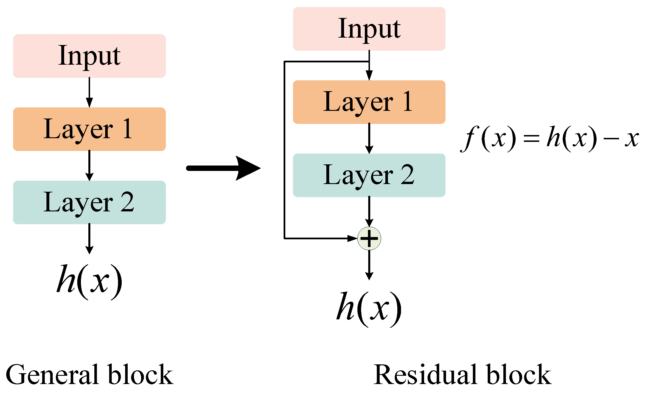
By stacking multiple residual units (RUs) with shortcut connections in the network, ResNet effectively addresses the degradation of deep neural network models. Each RU in ResNet can be thought of as a small neural network with skip connections, the basic structure of which is shown in Figure 1. The purpose of training a neural network is to build a model with an objective function of , and in the iteration of ResNet, the network will be forced to model due to the presence of short-circuit connections, a process known as residual learning. Compared with the traditional training process of neural networks, the advantages of residual learning are mainly reflected in the following three aspects. Firstly, because of the network’s initialization, the output of the traditional network in the initial training stage is mostly close to 0, while under the action of short connections, the output of ResNet is close to its input, that is, ResNet is equivalent to modeling the identity function at the initial training stage. This feature means that, when the objective function is remarkably close to the identity function, the speed of training the model can be greatly accelerated. Secondly, in the case of short connections, even if the individual layer of the network has not been effectively learned, it will not have much impact on the learning process of the entire network. Thirdly, in the process of backpropagation, using short connections, the gradient can be easily propagated throughout the network, effectively solving the problem of disappearing or exploding gradients.
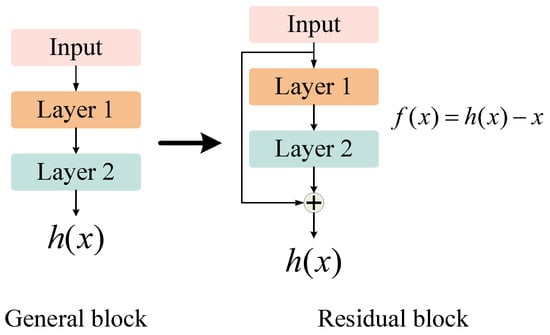
Figure 1.
Basic structure of the RU.
To facilitate the generalization of this research to engineering applications, this study made improvements based on ResNet-18, which has fewer parameters and a faster inference speed. On the one hand, the two-dimensional convolution layer and the pooled layer in the network were replaced by a one-dimensional convolution layer and a pooled layer, respectively, so that they could be transformed into 1D_ResNet, which can directly process one-dimensional vibration signals. On the other hand, compared with traditional methods of improving networks such as increasing the depth of the network or adding Dropout and ReLU to the network, this study referred to GoogLeNet’s Inception idea and added multiple branches using convolution nuclei of different sizes to the same level of the network. A wider network, M1D_ResNet, which can extract features at multiple scales, was constructed. The advantage of this improved network structure is that it not only reduces the difficulty of selecting the size of the convolution kernel but also further enhances the feature extraction capability of 1D_ResNet. Finally, to better meet the subsequent training of the SVDD model for detecting anomalies, the dimensions of the feature output of the M1D_ResNet model should not be too high. In this study, two fully connected layers were added after the last global average pooling layer, which were used to reduce the features’ dimensionality and the resulting output, and ultimately constituted the M1D_ResNet algorithm proposed in this study.
- (1)
- The convolution layer and the pooling layer
The convolution layer consists of a set of convolution nuclei, which work by dividing the image into small chunks called receptive fields to facilitate the extraction of features from the image. The kernel uses a set of specific weights to conduct convolution operations on the feature vectors output by the previous layer. The output of each layer is the result of convoluting multiple input features. The mathematical model can be described as follows:
where is the input feature matrix, is the network of layer , is the convolution kernel, is the network bias, is the output of layer , and is the input of layer .
To prevent the model from overfitting, a pooling layer was added behind the convolution layer. Pooling is a form of non-linear subsampling that reduces the amount of computation by reducing the network’s parameters, which helps to extract the combinations of features. The input can be divided into different areas by the maximum pooling function through the non-overlapping rectangular box, and the maximum value in the pooling field is taken as the output. The transformation function of maximum pooling is expressed as
In this formula, represents the eigenvalue of the th eigenvector in the th layer, , represents the width of the pooling region, and represents the output value corresponding to the neurons in layer .
- (2)
- The fully connected layer
Unlike pooling and convolution, the fully connected layer maps the output features of the last pooling layer to the sample label space by means of non-linear mapping. This is specifically described as
where is the input feature vector, and and are the weight matrix and bias vector, respectively.
2.1.2. Principle of the SVDD Algorithm
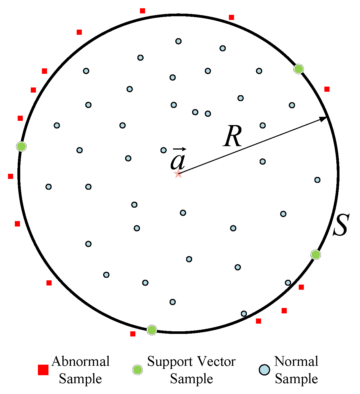
SVDD is a single-value classification method that uses a boundary method to solve problems. The basic idea of a description of the support vector data domain is to establish a closed region around the dataset, and adjust the region’s boundary by using different kernel functions, so that as many target samples as possible are included in the region, so as to realize the distinction between the target samples and the non-target samples [38]. Figure 2 shows the basic classification of the SVDD algorithm. In the figure, the solid circle is the target class of sample that needs to be described, the square is the abnormal sample that needs to be rejected, and is the spherical boundary of the described region. According to the figure, SVDD is the area covered by , determined by defining the center and the radius of the sphere. While completely covering the target sample, it also rejects the abnormal samples as much as possible.
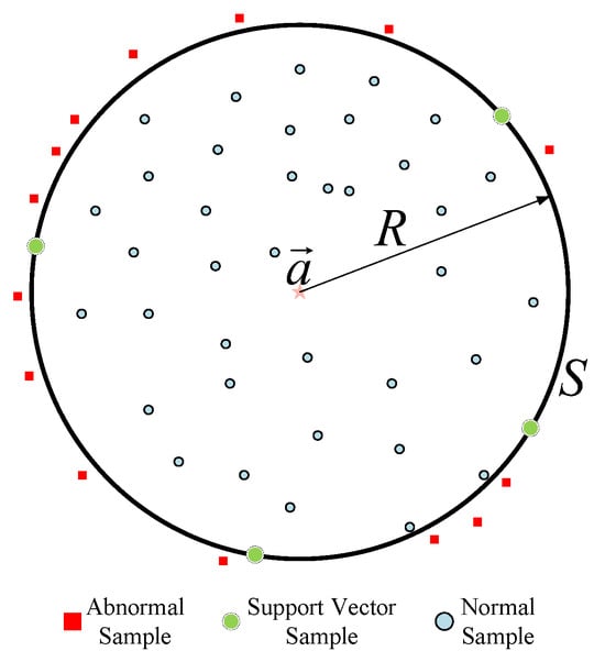
Figure 2.
Diagram of the SVDD method of detecting anomalies.
Suppose that vector is a column vector, and we have a training set of normal samples with the sample label . Our goal is to find the smallest hypersphere that can contain these samples, and this hypersphere model defines a closed boundary of the dataset, namely the hypersphere. The center and radius of the hypersphere are represented by and , respectively. This optimization problem is solved by minimizing on the premise that the hypersphere can contain all the training samples . For this purpose, the principle of minimizing the structural risk in statistical machine learning theory was adopted, that is, the following error functions were minimized:
The constraints can be expressed as
Considering that there may be abnormal data in the training set, the relaxation variable was introduced to accommodate the abnormal data to a certain extent. At the same time, a penalty factor was introduced to find the balance point between the hypersphere’s volume and the sample’s misclassification ratio. In general, the smaller is, the more sample points become the support vector, and the smaller the hypersphere that is formed. In this way, the above minimization problem transforms into
By introducing the Lagrangian function, Equation (6) transforms to
where the Lagrange coefficient is , .
The Lagrange function should be minimized with respect to , and , with the constraint that the partial derivative is equal to 0:
According to , , and Formula (10), when satisfies the following formula,
the Lagrange coefficient can be omitted, and Formulas (8)–(10) can be combined into
Equation (6) can be transformed into its dual form:
where is the kernel function, which is equivalent to the inner product of the samples in the feature space.
This formula can be calculated with KKT conditions, and the Lagrange coefficient corresponding to each sample can be obtained. The sample satisfying is called the support vector.
Finally, for the test sample , the distance from the center of the hypersphere is shown to be
If , it indicates that the test sample is on or inside the hypersphere and belongs to the class of normal samples; if , it is an abnormal sample.
2.2. A Method of Detecting Anomalies Based on M1D_ResNet and GA_SVDD
2.2.1. Method Workflow of This Study
To solve the problem that the existing feature extraction ability of 1D_ResNet is insufficient when processing the original one-dimensional vibration signal, this study proposed a three-channel M1D_ResNet algorithm to extract the state-sensitive features from the vibration signals at multiple scales. Then, the output of the last fully connected hidden layer of the M1D_ResNet algorithm was used as the feature set for training the SVDD model for detecting anomalies. In this process, to reduce the chance of artificially selecting SVDD hyperparameters, this study used GA to select the hyperparameters’ value. Finally, the anomaly-detecting algorithm combined with M1D_ResNet and GA_SVDD was verified in an experiment detecting the abnormalities in a hydraulically adjusted servomotor.
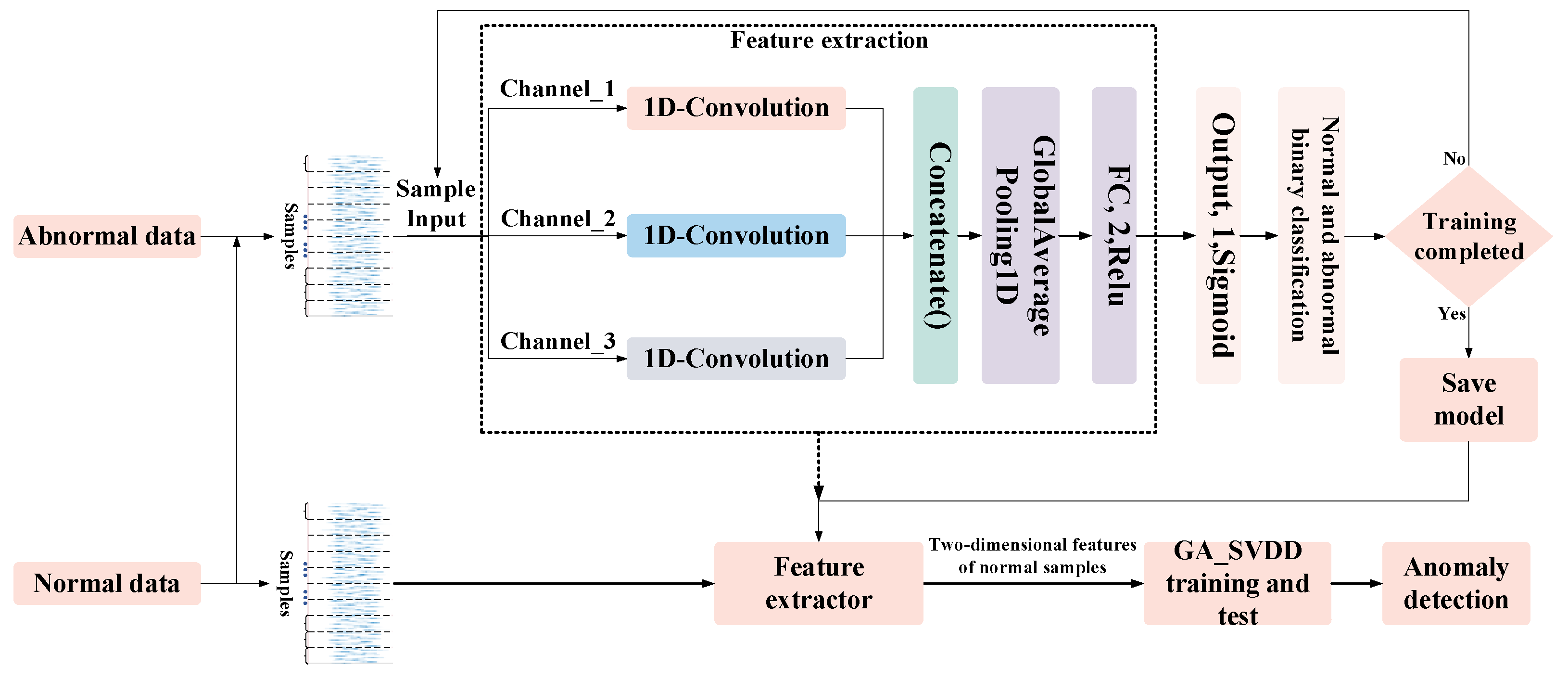
The process of detecting anomalies via this method based on M1D_ResNet and GA_SVDD is shown in Figure 3. It consists of three main parts: construction of the dataset, training and testing the M1D_ResNet feature extraction model, and training and testing the GA_SVDD anomaly-detecting model.
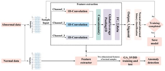
Figure 3.
Workflow of the method of this study.
(1) Building the dataset. The sample of one-dimensional original vibration signals was intercepted by a sliding window. After that, the dataset was divided into the training set, the verification set, and the test set by means of hierarchical sampling partitioning. The training, verification, and test sets used for M1D_ResNet contained the same number of normal and abnormal samples, while the training and verification sets used for the GA_SVDD algorithm only contained normal samples, and the test set was the same as the former.
(2) M1D_ResNet was trained to carry out binary classification of normal and abnormal states. When its effect on the test set was excellent, the feature extraction part of the model was considered able to accurately extract state-sensitive features in the samples, and the feature extraction layer of the trained M1D_ResNet model was extracted for constructing the feature set of the GA_SVDD algorithm.
(3) The training set and verification set with only normal samples were input into the M1D_ResNet feature extractor for feature extraction. The GA_SVDD algorithm was iterated and optimized by using the two-dimensional features output from the final fully connected layer. Finally, the anomaly-detecting model was evaluated regarding its performance in generalization with the test set containing both normal and abnormal samples.
2.2.2. The M1D_ResNet Model’s Structure and Parameter Settings
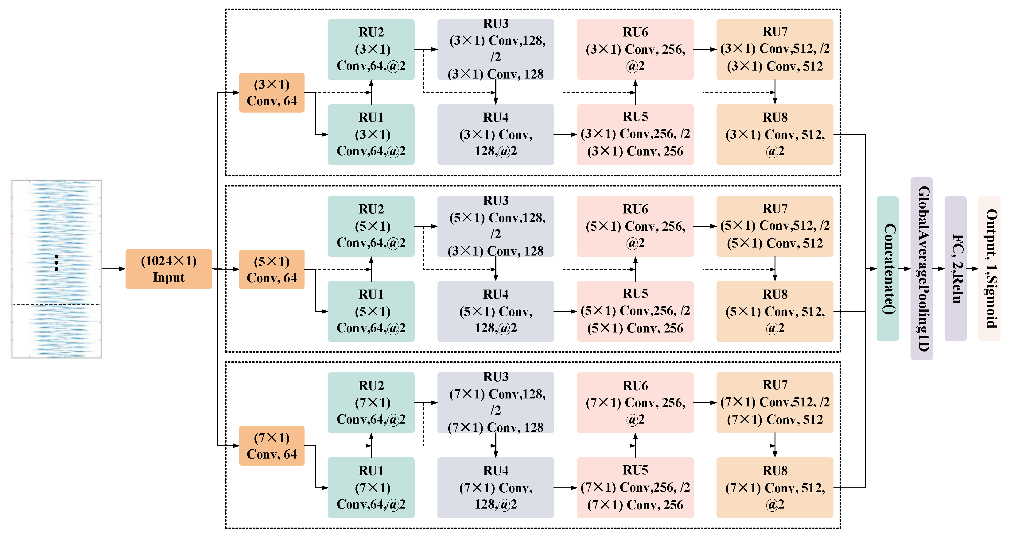
In fully extracting the multi-scale features of one-dimensional vibration signals, the ability of the traditional 1D_ResNet to extract features is weak, and the size of the convolution kernel is difficult to determine. In this study, the original single channel was improved into three channels, and different sizes of convolution kernels were used in different channels, and the size of the convolution kernels inside each channel were consistent. The network’s structure is shown in Figure 4.
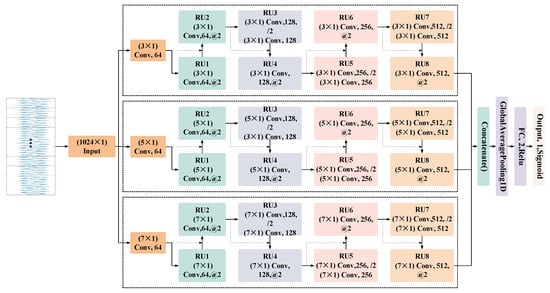
Figure 4.
Structure of the M1D_ResNet network.
Specifically, the samples input into the network on the leftmost side were fed into three channels. Each channel was composed of a convolution layer with the same size convolution kernels and eight RUs. Every two RUs, the number of convolution cores was doubled, while the size of the output features’ graph space was halved. From top to bottom, the sizes of the convolution kernel of each channel were 3 × 1, 5 × 1, and 7 × 1, which were used to extract more diverse features at different scales. The concatenation layer was used to integrate the features extracted from the three channels, and the global average pooling layer was added to reduce the features’ dimensions and the number of network parameters. After that, there was a fully connected feature output layer with two neurons, and the output two-dimensional features could be directly used in the construction of the GA_SVDD model. This was convenient for visualizing the distribution of the samples of features and the decision boundary of the SVDD hypersphere model, and could intuitively display the fitting effect of the SVDD model. Finally, there was an output layer of neurons and its sigmoid activation function, which could realize the binary classification of normal and abnormal states by matching the binary cross-entropy loss function. It should be noted that the internal structure of all RUs in the M1D_ResNet network, such as the batch normalization layer, the pooling layer, and the ReLU activation function, was the same as that of the residual units in 1D_ResNet, except for the size of the convolution kernel.
2.2.3. GA Optimization of the SVDD Process (Including Specific Parameter Settings)
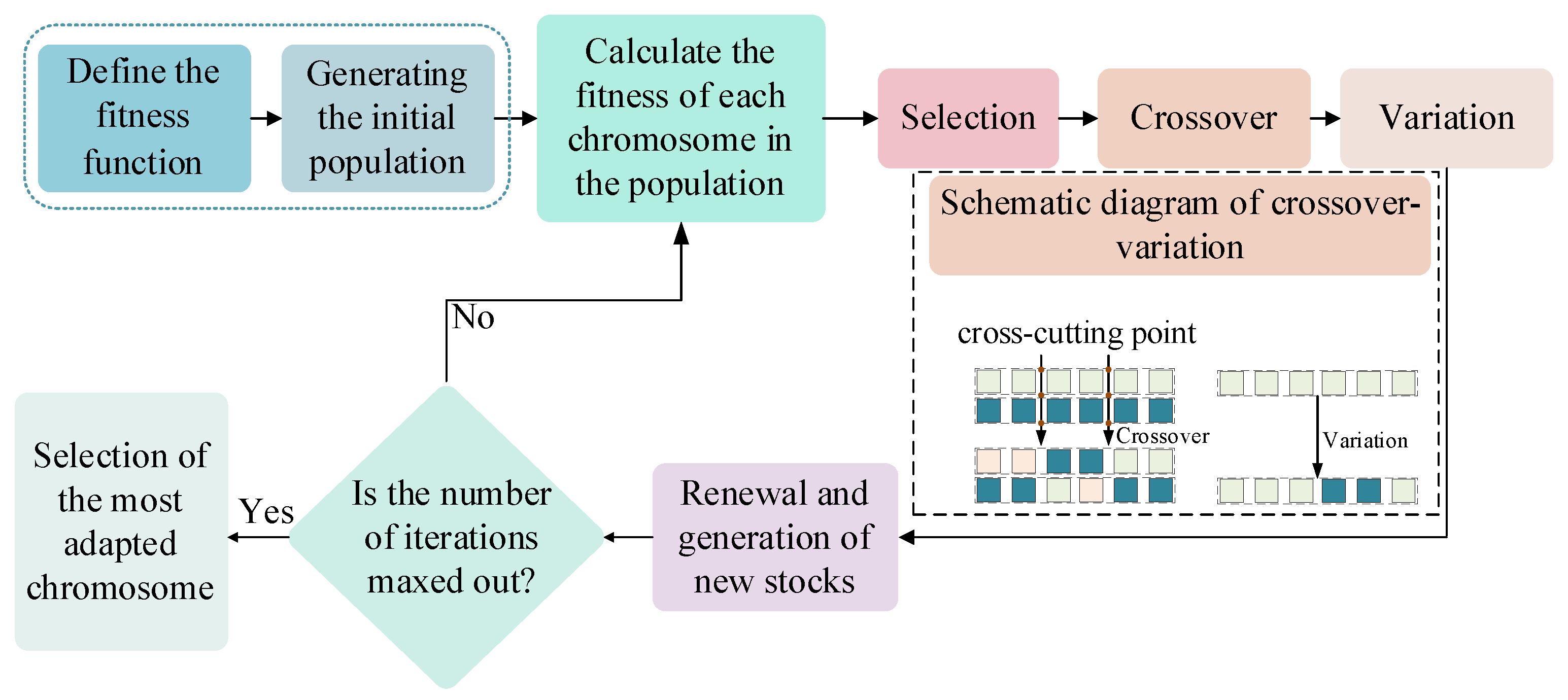
The SVDD itself has a hyperparameter: the positive case penalty factor . At the same time, the radial basis kernel function was selected to solve the problem of the linear indivisibility of low-dimensional features. The value of its gamma hyperparameter needed to be determined, and the number of hyperparameters increased to 2. To obtain the optimal solution of these hyperparameters, the GA was used in this study. The specific process of the GA’s optimization of the SVDD hyperparameters is shown in Figure 5.
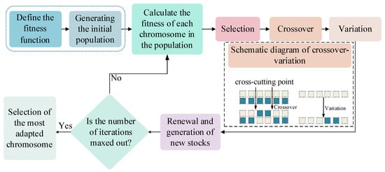
Figure 5.
Flow chart of the genetic algorithm used for optimization.
Step 1: To define the fitness function of the GA, Assuming that the accuracy (the total number of correct predictions/total number of predictions) of the SVDD model for the validation set was , define the fitness value of the GA as , and the iterative goal of the GA was to minimize the fitness value of chromosomes in the validation set.
Step 2: Encode a binary hyperparameter combination (, gamma) into a chromosome, where the values of the parameters and gamma are in the range [0.0001, 10]. Then, randomly generate an initial population with 500 chromosomes was, and set the maximum number of iterations to 100. The crossover_2point_bit crossover mechanism was adopted, and the mutation probability was set to 0.001.
Step 3: Initialize the SVDD model based on the chromosomes in the population, then train the model on the training set, and obtain the fitness values of each chromosome from the verification set.
Step 4: Use the fast tournament selection strategy to select chromosomes that enter the next generation of the population, and cross and mutate the chromosomes according to the two-point crossover strategy and the probability of mutation, and add the newly generated chromosomes to the next generation’s population. Then, renew and create new populations.
Step 5: Determine whether the maximum number of iterations is reached. If no, return to Step 3. If yes, proceed to Step 6.
Step 6: Calculate and select the chromosome with the highest fitness value in the new population, decode it into a combination of hyperparameters, and then initialize the SVDD model. Finally, retrain the model on the training set and the verification set, and calculate the accuracy value of the model using the test set.
3. Experimental Verification
To validate the effectiveness of the anomaly-detecting method based on M1D_ResNet and GA_SVDD in detecting the abnormal state of hydraulically adjusted servomotors, this study designed and conducted experiments using a test bench for simulating faults in a high-pressure hydraulically adjusted servomotor, as shown in Figure 6. The structure of the hydraulically adjusted servomotor consisted of a single-side acting symmetrical cylinder, primarily composed of springs, electro-hydraulic servo valves, throttle orifices, oil filters, displacement and pressure sensors, electrical junction boxes, and a valve block for installing quick-closing solenoids and cartridge check valves. Specifically, the pressure sensor M3 was installed between the non-working chamber of the hydraulically adjusted servomotor and the B port of the cartridge valve; pressure sensor M4 was installed between the C0 throttle orifice and the working chamber; and pressure sensor M5 was installed between the D0 throttle orifice and the A port of the cartridge valve. They all using threaded installations. Regarding the vibration signals, since the piston rod moved reciprocally in a direction perpendicular to the end cover, the impact component of the signal collected by the z-axis accelerometer was more pronounced compared with that in the x and y directions; hence the z-axis accelerometer was used as the data source in this study.
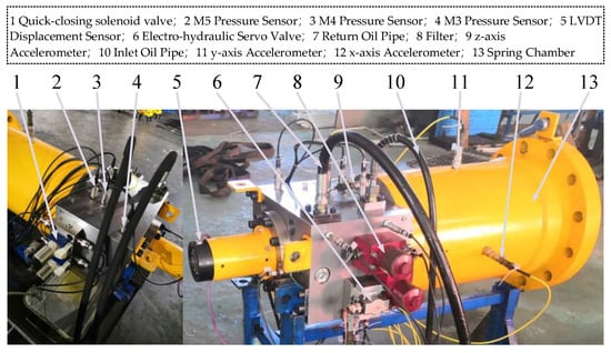
Figure 6.
Test bench for simulating faults in a high-pressure hydraulically adjusted servomotor.
3.1. Signal Acquisition
This study injected faults into the hydraulically adjusted servomotor by replacing faulty components or deliberately damaging normal parts, establishing nine types of faults, including internal leakage at the zero position in the electro-hydraulic servo valve, internal leakage in the solenoid valve (mild and severe), blockage before the solenoid valve’s throttle, blockage in the C0 throttle (mild and severe), internal leakage in the cylinder (mild and severe), and breakage of the spring in the hydraulically adjusted servomotor, as shown in Figure 7. Normally, the servo valve leaks at a rate of 0.70 L/min, but, when worn, it leaks at 12.32 L/min. Internal leakage faults of the solenoid valve were simulated by replacing valves to create mild and severe leakages; the normal diameter of the throttle’s hole before the solenoid valve is φ = 0.8 mm, which was reduced to φ = 0.5 mm in the simulations. The C0 throttle’s normal diameter is φ = 3 mm, which was adjusted to φ = 1 mm and φ = 2 mm to simulate mild and severe blockages, respectively. Leaks in the cylinder were simulated by varying the wear of the sealing rings, and breakage of the spring was simulated by either damaging the internal springs or partially cutting them.
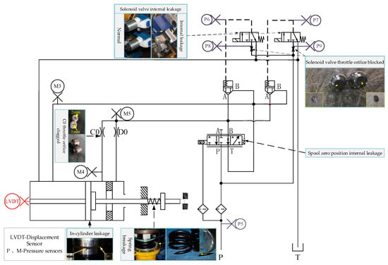
Figure 7.
Principles of the hydraulic system and establishment of faults for the hydraulically adjusted servomotor.
Finally, for describing the nine fault conditions and the normal condition, the EH oil supply system’s pressure was first adjusted to 15 MPa, and then the hydraulically adjusted servomotor was operated under a frequency of 0.1 Hz and 5% amplitude, which was controlled by LabVIEW. The sampling frequency was set to 12.5 kHz using Machine Condition Monitoring (MCM_2.1.2.0) software, with a duration of 30 s for each sample, and each condition was sampled three times. When making the dataset, the lengths of the sliding window and sliding step of the sample were set to 1024, and the samples were extracted from the vibration signals sequentially. The resulting experimental parameters are shown in Table 1.

Table 1.
Arrangement of the experimental data collection.
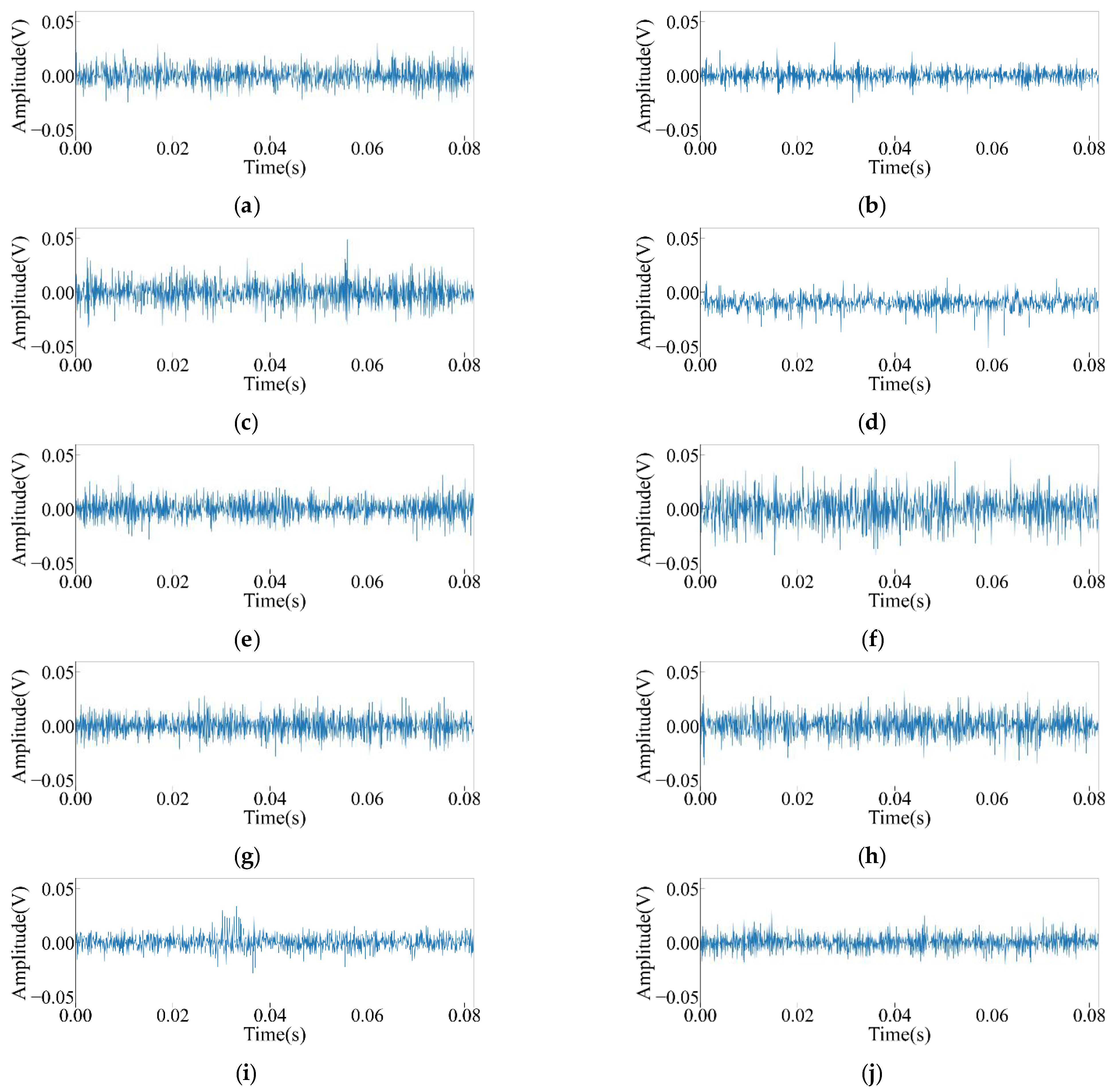
Figure 8 shows the time-domain diagram corresponding to a single sample of each state of the hydraulic servomotor (duration: 0.08192 s), where the vertical coordinate represents the amplitude of the voltage in V. It was found that the amplitudes of the three states of mild internal leakage in the cylinder, broken springs in the hydraulic servomotor, and the mildly blocked C0 throttle orifice were relatively small, and the time-domain signals of the broken spring of the hydraulic servomotor shifted to the negative half-axis of the vertical axis as a whole. The amplitude of leakage of the servo valve’s spool at the zero position was relatively large, and there were some differences in the waveforms of various states, which could be effectively distinguished by the diagnostic model.
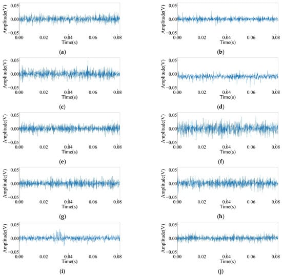
Figure 8.
Time-domain diagram of vibration signals in the z-direction for various types of faults in the throttle motor: (a) normal; (b) light in-cylinder leakage; (c) heavy in-cylinder leakage; (d) breakage of the spring; (e) blocking of the solenoid valve’s throttle orifice; (f) internal leakage of the servo valve’s spool at zero position; (g) light internal leakage of the solenoid valve; (h) heavy internal leakage of the solenoid valve; (i) light clogging of the C0 throttle orifice; (j) heavy clogging of the C0 throttle orifice.
3.2. Ablation Experiment
To validate the superiority of M1D_ResNet over the conventional 1D_ResNet and the effectiveness of each channel within M1D_ResNet, this study conducted a comparative study based on the principles of ablation experiments. M1D_ResNet was compared with the original 1D_ResNet, Channel_1 (retaining only the first channel), Channel_2 (retaining only the second channel), and Channel_3 (retaining only the third channel). It should be noted that although both the Channel_1 network and the original 1D_ResNet contained RUs with convolution kernels with a size of 3 × 1; the size of the kernels in their first convolutional layer and the configurations of the final output layer differed.
All the experiments and analyses for this study were conducted on the same computer with the following specifications: Intel Core i5-12400F (2.50 GHz), 32 GB RAM, and NVIDIA GeForce RTX 3060Ti (8 GB). The development environment consisted of scikit-learn 0.24.2, tensorflow-gpu 2.6.0, and Python 3.6.13.
3.2.1. Settings of the Ablation Hyperparameters
In this study, the same hyperparameter settings were used for training each algorithm, as shown in Table 2. To enhance the stability of the model during training, this study used a simple and reliable SGD optimizer to update the model’s parameters, setting the learning rate at 0.001. Additionally, a smaller batch size of 32 was adopted to refine the iteration process of the model, and the number of epochs was set to 150 to ensure that the model was adequately trained.

Table 2.
Hyperparameter settings for training the model.
3.2.2. Analysis of the Results of the Ablation Experiment
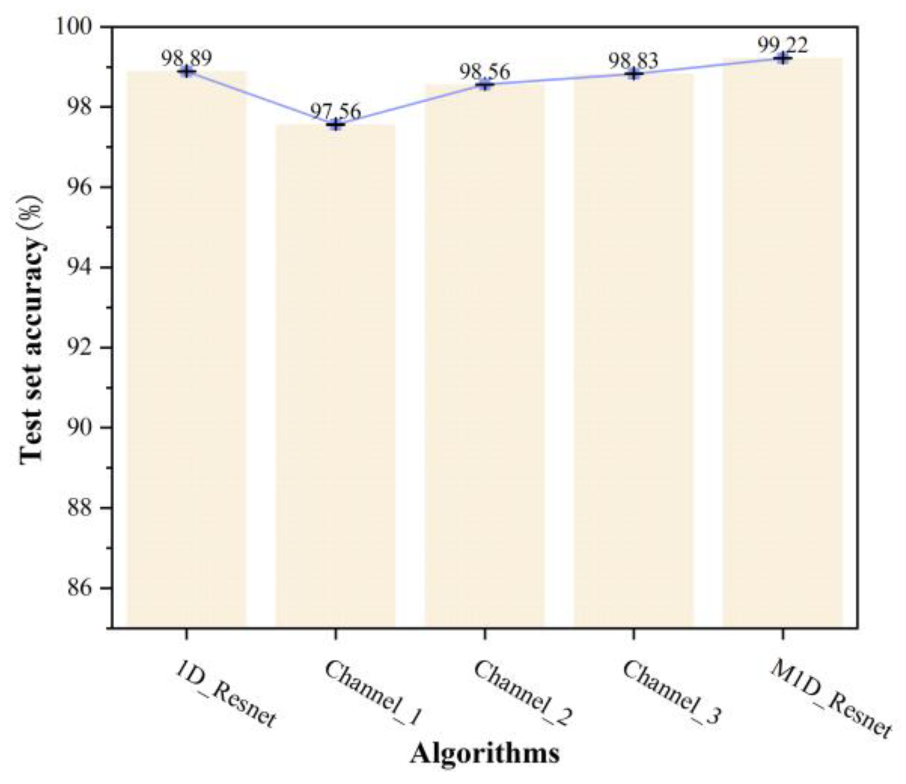
On the basis of the hyperparameter settings described above, to eliminate the impact of the division of the dataset on the experimental outcomes, this study conducted fivefold cross-validation for M1D_ResNet and four other algorithms. During the cross-validation process, the dataset was first shuffled to enhance the model’s capabilities for generalization. Then, in each iteration, stratified sampling was used to allocate 80% as the training set and the remaining 20% as the test set. The mean and standard deviation of the accuracy metrics for each model on the test set are displayed in Figure 9.
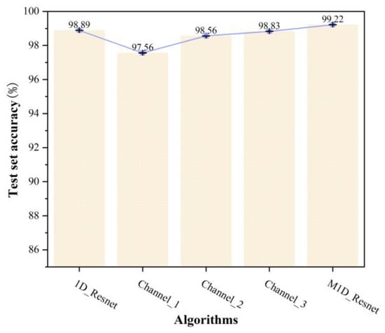
Figure 9.
Mean and standard deviation of the accuracy of cross-validation for each algorithm.
As can be seen from Figure 9, M1D_ResNet had the highest mean accuracy, followed by 1D_ResNet, Channel_3, and Channel_2. Channel_1 not only had the lowest mean accuracy but also the highest standard deviation, indicating that it performed the worst during the fivefold cross-validation process. In the case of 1D_ResNet, it initially used a convolution layer with a kernel with a size of 7 × 1 to capture the spatial context of the initial input across a large receptive field, followed by a smaller (3 × 1) kernel to capture the local features in a smaller receptive field. This global-to-local network structure and the choice of the kernels’ sizes provided strong capabilities for feature extraction, making its accuracy second only to M1D_ResNet. However, the other three single-channel networks had kernels of only one size, which did not adequately address both the global and local features, leading to less effective classification. The trend of mean accuracy decreasing from Channel_3 to Channel_2 to Channel_1 indicated that the state-sensitive features of the hydraulically adjusted servomotor’s vibration signals needed to be extracted from larger receptive fields, as smaller kernels tended to lose information on significant features. Finally, these results strongly supported the superiority of M1D_ResNet, which directly extracted and fused global and local features across multiple channels from the raw samples, compared with the global-to-local structure of 1D_ResNet. The local features in 1D_ResNet were extracted on the basis of the global features, which inevitably involved some loss of information. In contrast, M1D_ResNet’s local features were directly extracted from the raw samples, avoiding the loss of information. Furthermore, M1D_ResNet incorporated kernels with a size of 5 × 1, thus enriching the feature information further.
To analyze and demonstrate the specific training processes of each model, this study selected the cross-validation process corresponding to the accuracies closest to the mean for each algorithm, and the curves of training loss and accuracy are shown in Figure 10.

Figure 10.
Curves of training loss and accuracy for each algorithm.
As shown in Figure 10a, M1D_ResNet exhibited the fastest decrease in training loss, approximately converging to the minimum value in around 30 epochs. Compared with other algorithms, it demonstrated smaller fluctuations in training loss throughout the training process, maintaining a minimal loss, thereby reflecting the superior performance of M1D_ResNet. Although Channel_3 converged slowly at the beginning, it tended to stabilize at around 60 epochs. In contrast, Channel_2 showed the slowest convergence. Figure 10b reveals that the algorithms reflected the same convergence trend as the training loss in terms of training accuracy, and it can be seen from their localized plots that although the accuracy of each algorithm fluctuated during the training process at the later stage, the fluctuation of M1D_ResNet was the smallest and basically stayed at the highest level. If we also consider Figure 9, it can be seen that the accuracy of M1D_ResNet was similar on both the training and test sets; therefore, the model did not suffer from overfitting in any of the training processes, which fully explained its network’s structure as well as the reasonableness of the training hyperparameters.
In addition, to visualize the size and inference speed of each model, this study selected three key performance indicators, namely, the number of parameters, the amount of computation, and the inference time of the model on a single sample, for a comparative analysis. The number of parameters, as an inherent attribute of the model itself, reflects the amount of disk storage space required by the model. Computation FLOPs, on the other hand, reflect the complexity of the model and the consumption of resources during the actual inference process, and this metric was determined with fixed input data. The inference time for a single sample, on the other hand, reflects the actual processing speed of the model for a specific sample. In light of this, this study used the test set of the hydraulically adjusted servomotor’s vibration signals 10 times for each algorithm, and the average value of each index was taken, which are summarized in Table 3.

Table 3.
Comparison of the size and inference speed of the models.
According to Table 3, considering that the size of most of the convolutional kernels in 1D_ResNet was the same as that in Channel_1, the performances of 1D_ResNet and Channel_1 were basically comparable across the three metrics. For the other three models, as the size of the convolutional kernel increased and the number of network branches increased, the number of parameters of the model, the amount of computation, and the average time consumed to process a single sample also increased incrementally. Although the M1D_ResNet model proposed in this study did not have an advantage over the other four single-scale networks in terms of the model’s size and inference speed, its significant improvement in diagnostic performance as well as its stability in training could achieve a higher accuracy with complex and diverse datasets, which, in turn, reduced the number of false alarms and omissions, and ultimately improved the reliability and safety of the fault diagnosis system. Meanwhile, M1D_ResNet automatically extracts features with a dimension of only two, which is extremely convenient compared with the traditional manual feature extraction in the time and frequency domains, as well as the cumbersome process of feature selection.
3.2.3. Comparison of the Capabilities of Different Algorithms for Feature Extraction
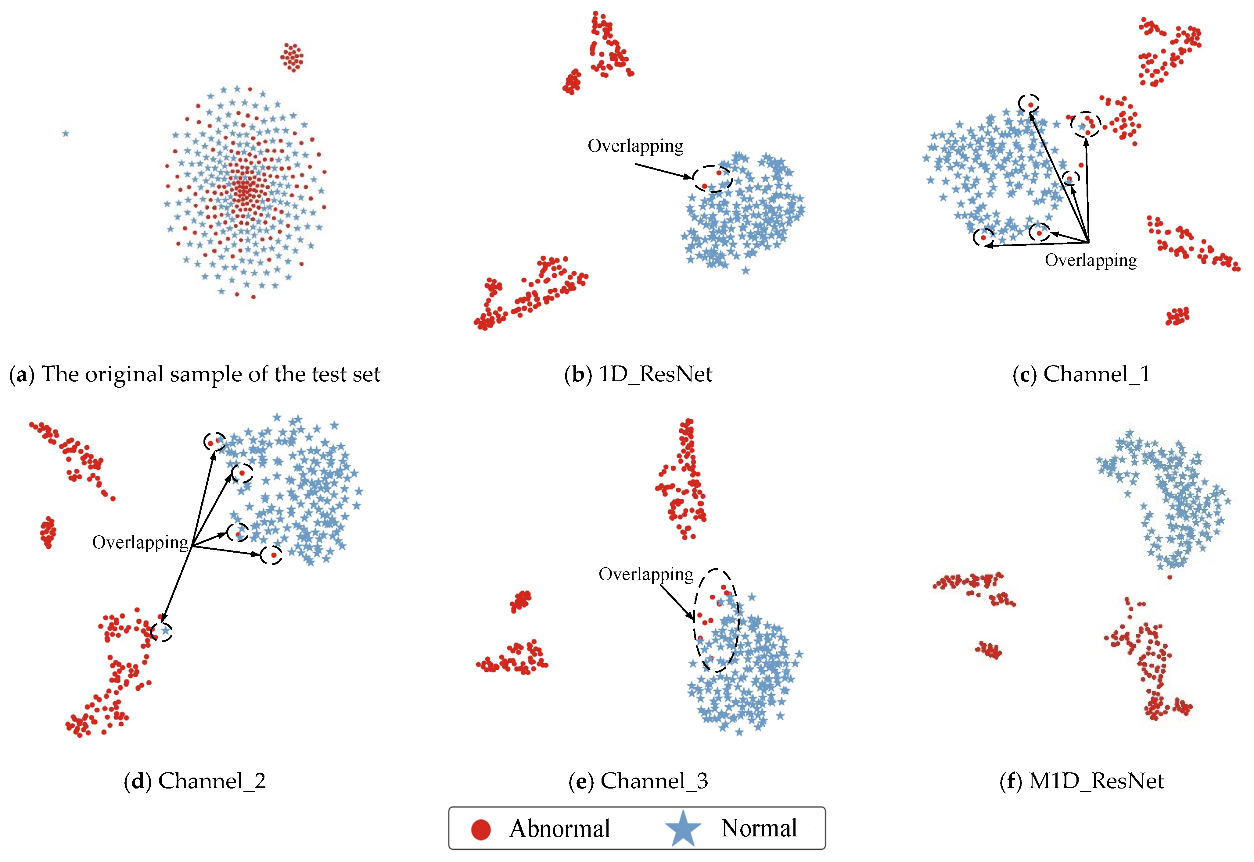
The persistent issue of “black boxes” in deep learning makes it difficult to understand and explain the internal workings of networks. To investigate the learning methods and capabilities of M1D_ResNet and its comparative algorithms for feature extraction, this study re-sampled the dataset into training, validation, and test sets in a 3:1:1 ratio for training and testing each model. Subsequently, t-SNE was used to reduce the dimensionality and visualize the original samples from the test set. Finally, for the comparative analysis, the trained models were used to make predictions on the test set. This allowed for collection of the feature data output by the global average pooling layer during the forward propagation process of each network, which were then subjected a reduction in dimensionality and visualization using the t-SNE algorithm. The results are shown in Figure 11.

Figure 11.
Visualization of the raw data and features of each model.
From Figure 11a, it is evident that the original normal and abnormal samples in the test set were severely mixed. However, as can be seen in Figure 11b–f, after the feature extraction process of each model, the samples of the two states could basically be distinguished. However, except for the proposed M1D_ResNet algorithm, the feature distributions of the other algorithms still showed varying degrees of overlap, reaffirming the strong feature extraction capability of M1D_ResNet. Among these, 1D_ResNet exhibited the least overlap in the features’ distributions, while the features extracted by Channel_1 showed the most significant overlap. Additionally, the clustering centers of the two states were remarkably close, which can lead to poor classification performance, consistent with the conclusions drawn from Figure 9.
3.3. Experimental Analysis of GA-SVDD
3.3.1. Arrangement of the Experimental Data of GA-SVDD
The feature extraction part of the trained M1D_ResNet model was used as the feature extractor for the GA-SVDD algorithm. By extracting features from samples of various categories, data samples with a dimensionality of two were obtained. Normal samples were divided into the training, validation, and test sets in a 3:1:1 ratio. Additionally, when conducting tests on the performance of the SVDD model in generalization using samples from various categories, it was essential to ensure that the total numbers of normal and abnormal samples in the test set were balanced and that the numbers of each type of abnormal sample were equal. The final experimental data for GA-SVDD are presented in Table 4.

Table 4.
Arrangement of the experimental data for GA-SVDD.
3.3.2. Analysis of the Hyperparameter Optimization Process of GA-SVDD
The features extracted from the training and validation sets were used for training the SVDD hypersphere model and for optimization of the hyperparameters. The specific process of GA-based optimization of the hyperparameters for the SVDD is illustrated in Figure 12.

Figure 12.
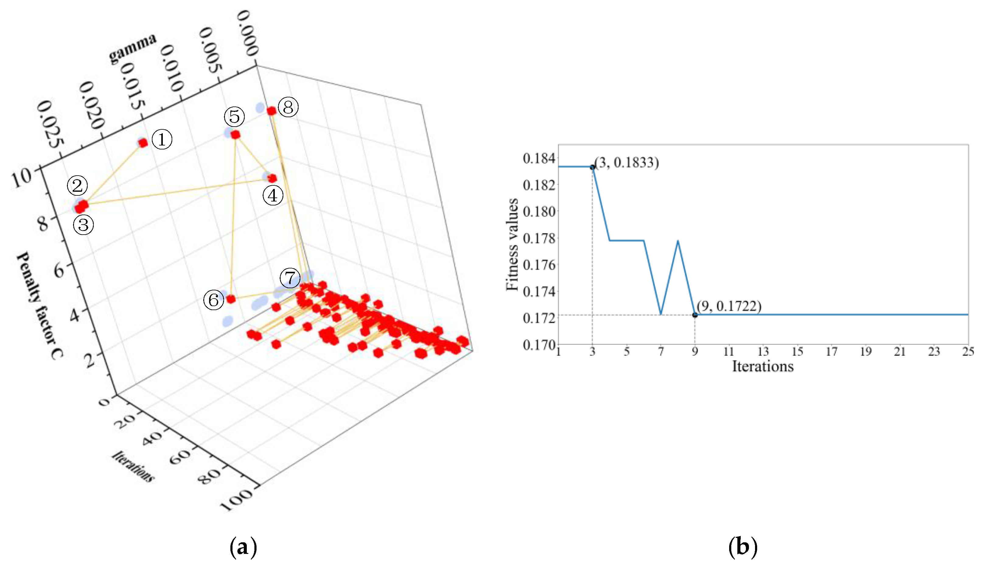
The GA optimization process. (a) Process of optimizing the parameters. The red squares indicate the combinations of hyperparameters obtained in a certain iteration, and the combinations of hyperparameters obtained in the first eight iterations are indicated by 1–8, respectively; the dots indicate the specific values of the penalty factor C and the gamma parameter in the combinations of hyperparameters. (b) Changes in the fitness values.
The GA performed 100 iterations on the hyperparameters of SVDD. Figure 12a shows the combinations of hyperparameters with the highest fitness values selected by the GA after each iteration. It is evident that in the initial iterations, the changes in the two hyperparameters were significant, indicating that the GA was searching for the global optimum. As the iterations progressed, after only seven iterations, the two hyperparameters largely converged to the global optimum, particularly the penalty factor, which remained almost unchanged throughout the process. Figure 12b shows that the fitness function values displayed a strong downward trend in the first seven iterations, indicating continuous improvement in the accuracy of the SVDD model and demonstrating the powerful optimization capability of the GA. At the eighth iteration, Figure 12b shows a significant fluctuation in the fitness value. Observation of Figure 12a reveals that this was because the combination of hyperparameters deviated from the area of the global optimum, but it returned to be close to the global optimum in the subsequent (ninth) iteration. In subsequent iterations, the combination of hyperparameters oscillated near the global optimum, with a decreasing amplitude. However, the fitness values had already converged to a minimum and remained unchanged, which is reasonable, considering the limited effect of fine-tuning the SVDD hypersphere’s boundaries through the penalty factor and the kernel parameter gamma. A combination of hyperparameters was finally selected and the specific attributes of the SVDD hypersphere trained on the training set and validation set are shown in Table 5.

Table 5.
Final hyperparameters and attributes of the SVDD model.
3.3.3. Analysis of SVDD’s Effect on Detecting Anomalies
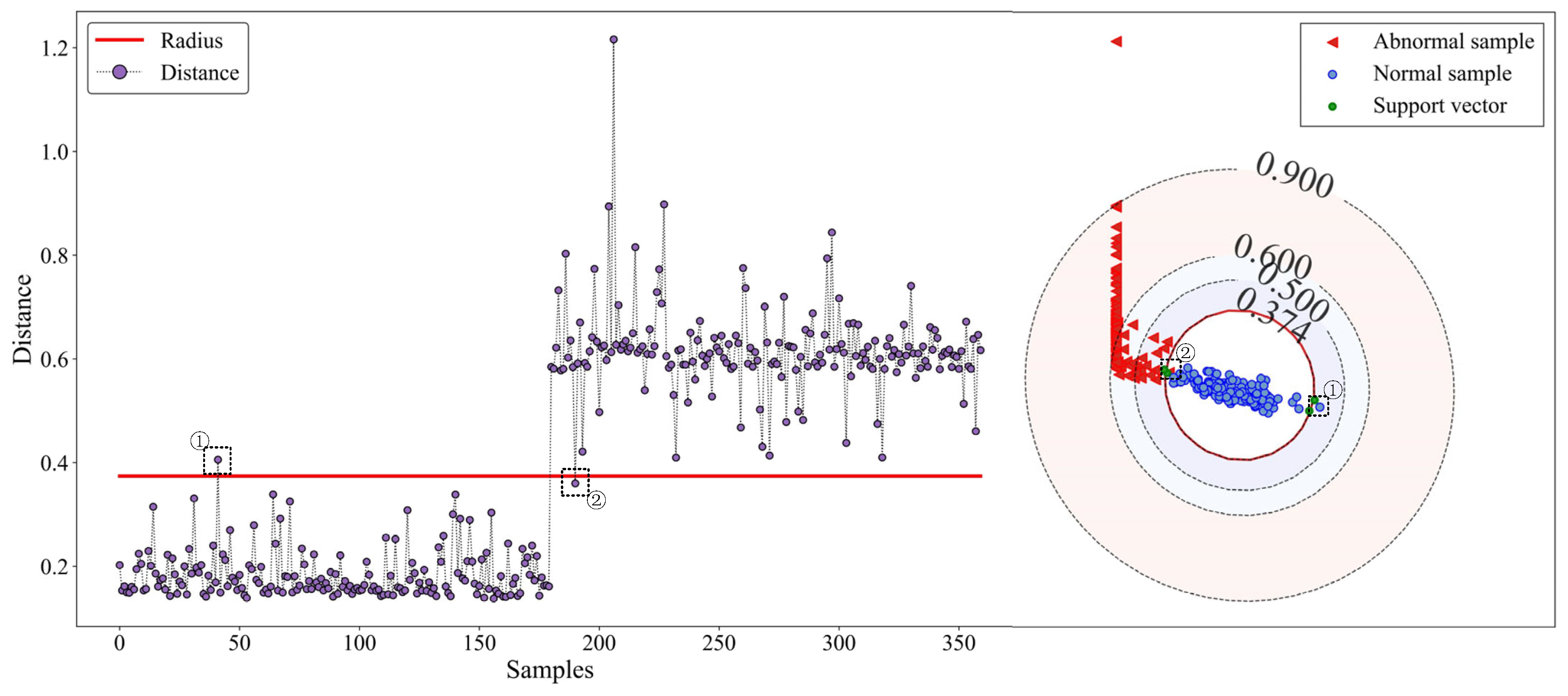
To visually demonstrate the performance of the SVDD anomaly-detecting model trained in the previous section, we evaluated it on the test set. Initially, the distance–radius curve and decision boundaries of the model on the test set were plotted, as shown in Figure 13. From the radius–distance curve on the left side of Figure 13, it can be observed that the normal and abnormal samples were generally distributed on either side of the radius line. Only one normal sample was located above the radius line, and only one abnormal point was below it. The spatial positions of these two misjudged samples are shown on the right side of Figure 13. A mild fault is not much different from the normal state, which inevitably leads to a closer distribution of the samples with a normal state, so it led to two misjudgments by the model; however, on the whole, the model still made a good distinction between these two states, which verified the applicability of the SVDD model in the field of detecting abnormalities in hydraulically adjusted servomotors.
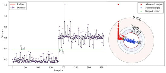
Figure 13.
Diagram of the distance–radius curve and the decision boundary: ① misclassified normal samples; ② misclassified abnormal samples.
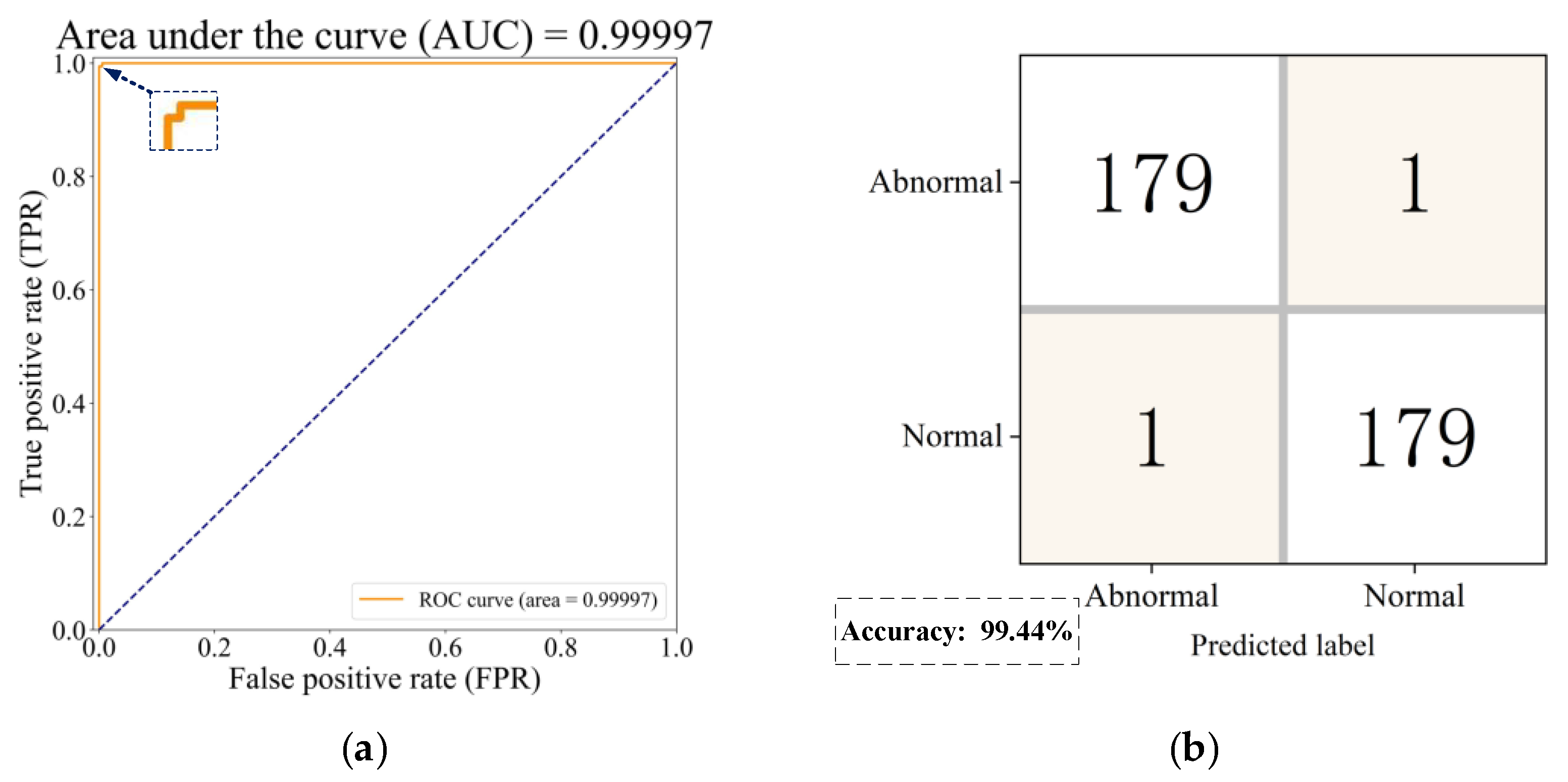
Figure 14a shows the ROC curve of the current SVDD model on the test set. The AUC did not reach 1 because there was a small zigzag in the upper left corner of the ROC curve, but the AUC of 0.99997 indicated that the model’s performance in detecting faults was already excellent, which verified the superiority of the GA in optimization to search for the hyperparameters of SVDD. Figure 14b shows a confusion matrix that yielded the same results as Figure 13, with an overall model accuracy of 99.44%.
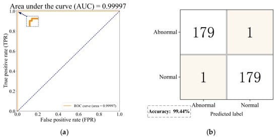
Figure 14.
Tests of the SVDD model’s performance: (a) receiver operating characteristic curve; (b) confusion matrix.
In addition, to visualize the inference speed of the SVDD model, this study ran the trained SVDD model on the test set 10 times, and the statistics of the time consumed by the model during the inference of a single sample are shown in Table 6. If we consider these results alongside those in Table 3, the processing speed of the SVDD model, a traditional machine learning model, was much faster than M1D_ResNet, and the time it consumed for processing small datasets was negligible.

Table 6.
Testing time of the SVDD model for a single sample.
4. Conclusions
This study introduced M1D_ResNet for extracting the features of the operational states of high-pressure hydraulically adjusted servomotors, addressing the issue of the traditional 1D_ResNet failing to adequately extract features at different scales. Subsequently, features extracted from the vibration signals of the hydraulically adjusted servomotor during normal operation using M1D_ResNet were used to construct a model for detecting anomalies in a hydraulically adjusted servomotor using SVDD, meeting the needs of practical engineering applications to build such models on the basis of normal data alone. Additionally, the GA was used to automatically optimize the hyperparameters of SVDD, addressing the issue of needing manual intervention for adjusting the hyperparameters. The conclusions are as follows:
(1) Compared with the traditional 1D_ResNet and three other single-scale one-dimensional residual networks, M1D_ResNet achieved the highest classification accuracy. The feature learning effects of each network were analyzed visually using t-SNE, revealing that M1D_ResNet’s feature learning was superior to that of the other networks.
(2) The iterative paths of combinations of hyperparameters during the GA optimization process were visually analyzed, demonstrating that GA could effectively optimize the hyperparameters of SVDD.
(3) Experimental validation was conducted on the SVDD-based detection of anomalies for hydraulically adjusted servomotors, and the decision boundaries were visualized, proving the effectiveness of the SVDD hypersphere model in detecting anomalies in hydraulically adjusted servomotors in different operational states. This lays a solid foundation for constructing models for detecting anomalies in hydraulically adjusted servomotors in practical engineering applications based solely on normal data.
In the future, in-depth research on methods of fusing multi-source information based on vibration and pressure signals can be conducted to improve the accuracy of detecting anomalies in adjusted hydraulic servomotors. In addition, research on reducing the weight of the M1D_ResNet network could be conducted to reduce the size of the model and improve its operational efficiency.
Author Contributions
Conceptualization, X.Y.; data curation, X.Y. and E.T.; formal analysis, A.J.; methodology, X.Y.; project administration, W.J.; resources, W.J.; software, X.Y. and Y.Z.; supervision, W.J.; validation, E.T. and Z.Q.; visualization, Y.Z.; writing—original draft, X.Y.; writing—review and editing, A.J. All authors have read and agreed to the published version of the manuscript.
Funding
This research was supported by the National Natural Science Foundation of China (Grant No. 52275067) and the Province Natural Science Foundation of Hebei, China (Grant No. E2023203030).
Informed Consent Statement
Informed consent was obtained from all subjects involved in the study.
Data Availability Statement
The data presented in this study are available on request from the corresponding author due to privacy.
Conflicts of Interest
The authors declare no conflicts of interest.
References
- Li, T. Development and prospect of turbine fault diagnosis technology. Equip. Maint. Technol. 2019, 14. [Google Scholar] [CrossRef]
- Li, Y.; Lu, Z.; Liang, X.; Zhou, Y. Analyzing the causes of internal leakage defects in the main regulator and their treatment. Equip. Manag. Maint. 2020, 33–34. [Google Scholar]
- Mu, X. Research on Servo Control, Performance Test and Reliability of Hydraulic Servomotor. Master’s Thesis, Shanghai Jiao Tong University, Shanghai, China, 2018. [Google Scholar]
- Jin, S.X.; Wu, S.L.; Zhang, Z.Y.; Tong, M.F.; Wang, F.L. Analysis of the causes of faulty load shedding and overspeed tripping of heating units. Power Eng. 2002, 2034–2039. [Google Scholar]
- Yu, D.; Xu, J. Simulation analysis of the effect of insensitivity of turbine regulation system on system performance. Power Eng. 1991, 46–52+67–68. [Google Scholar]
- Yu, D.; Xu, J.-Y.; Li, Y.-W. Model-based fault detection in hydraulic speed control system of steam turbine. Chin. J. Electr. Eng. 1993, 64–69. [Google Scholar] [CrossRef]
- Li, W.Z. Research on Networked Fault Diagnosis System for Turbine Regulation System. Master’s Thesis, North China Electric Power University, Beijing, China, 2000. [Google Scholar]
- Wang, Q. FMEA and FTA Based Fault Diagnosis and Its Application in DEH System. Master’s Thesis, North China Electric Power University (Beijing), Beijing, China, 2004. [Google Scholar]
- Wang, X.; Li, X.; Li, F. Analysis on Oscillation in Electro-Hydraulic Regulating System of Steam Turbine and Fault Diagnosis Based on PSOBP. Expert Syst. Appl. 2010, 37, 3887–3892. [Google Scholar] [CrossRef]
- Xu, P. Model-Based Fault Diagnosis of Turbine Regulation System. Master’s Thesis, Harbin Institute of Technology, Harbin, China, 2011. [Google Scholar]
- Feng, Y.X.; Cai, S.; Song, C.M.; Wei, S.J.; Liu, J.F.; Yu, D.R. The Research of the Jam Fault Features and Diagnostic Methods of the Slide Valve Oil Motive Based on DEH Data. Adv. Mat. Res. 2013, 860–863, 1791–1795. [Google Scholar] [CrossRef]
- Zhang, Z. Development of Turbine Oil Supply Control System and Hydraulic Servomotor Fault Diagnosis. Master’s Thesis, Dalian University of Technology, Dalian, China, 2019. [Google Scholar]
- Gawde, S.; Patil, S.; Kumar, S.; Kamat, P.; Kotecha, K.; Abraham, A. Multi-Fault Diagnosis of Industrial Rotating Machines Using Data-Driven Approach: A Review of Two Decades of Research. Eng. Appl. Artif. Intell. 2023, 123, 106139. [Google Scholar] [CrossRef]
- Yang, X.; Jiang, A.; Jiang, W.; Zhao, Y.; Tang, E.; Chang, S. Abnormal Detection and Fault Diagnosis of Adjustment Hydraulic Servomotor Based on Genetic Algorithm to Optimize Support Vector Data Description with Negative Samples and One-Dimensional Convolutional Neural Network. Machines 2024, 12, 368. [Google Scholar] [CrossRef]
- Zhou, W.J.; Hu, Y.H.; Tang, J. Research on early warning of hydraulic servomotor failure based on support vector data description. Thermal Turbine 2022, 51, 290–294. [Google Scholar] [CrossRef]
- Jiang, W. Intelligent Information Diagnosis and Monitoring of Hydraulic Failures; Machinery Industry Press: Norwalk, CT, USA, 2013; ISBN 978-7-111-41583-1. [Google Scholar]
- Jiang, W.-L.; Zhao, Y.-H.; Zang, Y.; Qi, Z.-Q.; Zhang, S.-Q. Feature Extraction and Diagnosis of Periodic Transient Impact Faults Based on a Fast Average Kurtogram–GhostNet Method. Processes 2024, 12, 287. [Google Scholar] [CrossRef]
- Krizhevsky, A.; Sutskever, I.; Hinton, G.E. ImageNet Classification with Deep Convolutional Neural Networks. Commun. ACM 2017, 60, 84–90. [Google Scholar] [CrossRef]
- He, K.; Zhang, X.; Ren, S.; Sun, J. Deep Residual Learning for Image Recognition. In Proceedings of the 2016 IEEE Conference on Computer Vision and Pattern Recognition (CVPR), Las Vegas, NV, USA, 27–30 June 2016; pp. 770–778. [Google Scholar]
- Wang, H.; Dai, X.; Shi, L.; Li, M.; Liu, Z.; Wang, R.; Xia, X. Data-Augmentation Based CBAM-ResNet-GCN Method for Unbalance Fault Diagnosis of Rotating Machinery. IEEE Access 2024, 12, 34785–34799. [Google Scholar] [CrossRef]
- Liu, Z.; Guo, B.; Wu, F.; Han, T.; Zhang, L. An Improved Burr Size Prediction Method Based on the 1D-ResNet Model and Transfer Learning. J. Manuf. Process. 2022, 84, 183–197. [Google Scholar] [CrossRef]
- Tan, A.; Wang, Y.; Zhao, Y.; Zuo, Y. 1D-Inception-Resnet for NIR Quantitative Analysis and Its Transferability between Different Spectrometers. Infrared Phys. Techn. 2023, 129, 104559. [Google Scholar] [CrossRef]
- Liu, R.; Wang, F.; Yang, B.; Qin, S.J. Multiscale Kernel Based Residual Convolutional Neural Network for Motor Fault Diagnosis Under Nonstationary Conditions. IEEE Trans. Ind. Inform. 2020, 16, 3797–3806. [Google Scholar] [CrossRef]
- Pan, H.; Xu, H.; Zheng, J.; Tong, J.; Cheng, J. Twin Robust Matrix Machine for Intelligent Fault Identification of Outlier Samples in Roller Bearing. Knowl.-Based Syst. 2022, 252, 109391. [Google Scholar] [CrossRef]
- Pan, H.; Sheng, L.; Xu, H.; Tong, J.; Zheng, J.; Liu, Q. Pinball Transfer Support Matrix Machine for Roller Bearing Fault Diagnosis under Limited Annotation Data. Appl. Soft Comput. 2022, 125, 109209. [Google Scholar] [CrossRef]
- Moya, M.M.; Koch, M.W.; Hostetler, L.D. One-Class Classifier Networks for Target Recognition Applications. NASA STI/Recon Tech. Rep. N 1993, 93, 24043. [Google Scholar]
- Bishop, C.M. Novelty Detection and Neural Network Validation. In Proceedings of the ICANN ’93, Amsterdam, The Netherlands, 13–16 September 1993; Gielen, S., Kappen, B., Eds.; Springer: London, UK, 1993; pp. 789–794. [Google Scholar]
- Cabral, G.G.; Oliveira, A.L.I. One-Class Classification Based on Searching for the Problem Features Limits. Expert Syst. Appl. 2014, 41, 7182–7199. [Google Scholar] [CrossRef]
- Tax, D.M.J.; Duin, R.P.W. Support Vector Domain Description. Pattern Recognit. Lett. 1999, 20, 1191–1199. [Google Scholar] [CrossRef]
- Zou, Y.; Wu, H.; Guo, X.; Peng, L.; Ding, Y.; Tang, J.; Guo, F. MK-FSVM-SVDD: A Multiple Kernel-Based Fuzzy SVM Model for Predicting DNA-Binding Proteins via Support Vector Data Description. Curr. Bioinf. 2021, 16, 274–283. [Google Scholar] [CrossRef]
- Huang, C.; Min, G.; Wu, Y.; Ying, Y.; Pei, K.; Xiang, Z. Time Series Anomaly Detection for Trustworthy Services in Cloud Computing Systems. IEEE Trans. Big Data 2022, 8, 60–72. [Google Scholar] [CrossRef]
- He, Z.; Zeng, Y.; Shao, H.; Hu, H.; Xu, X. Novel Motor Fault Detection Scheme Based on One-Class Tensor Hyperdisk. Knowl.-Based Syst. 2023, 262, 110259. [Google Scholar] [CrossRef]
- Zhang, Y.; Du, Y.; Gao, Z.; Qin, Y.; Wei, X. PSO-SVDD Normal Domain-Based Hidden Bearing Disease Monitoring under Fault-Free Data Conditions. Mod. Manuf. Eng. 2019, 94–99, 107. [Google Scholar] [CrossRef]
- Xu, E.; Li, Y.; Peng, L.; Yang, M.; Liu, Y. An Unknown Fault Identification Method Based on PSO-SVDD in the IoT Environment. Alex. Eng. J. 2021, 60, 4047–4056. [Google Scholar] [CrossRef]
- Luo, D.; Xue, X. PSO-SVDD-based fault diagnosis of gearbox. Ship Electron. Eng. 2023, 43, 119–122. [Google Scholar]
- Bai, Q. Analysis of Particle Swarm Optimization Algorithm. Stud. Comp. Intell. 2010, 3, 180. [Google Scholar] [CrossRef]
- Guo, Y.; Xiao, H. Genetic Algorithm-Tuned Adaptive Pruning SVDD Method for HRRP-Based Radar Target Recognition. Int. J. Remote Sens. 2018, 39, 3407–3428. [Google Scholar] [CrossRef]
- Tax, D.M.J.; Duin, R.P.W. Support Vector Data Description. Mach. Learn. 2004, 54, 45–66. [Google Scholar] [CrossRef]
Disclaimer/Publisher’s Note: The statements, opinions and data contained in all publications are solely those of the individual author(s) and contributor(s) and not of MDPI and/or the editor(s). MDPI and/or the editor(s) disclaim responsibility for any injury to people or property resulting from any ideas, methods, instructions or products referred to in the content. |
© 2024 by the authors. Licensee MDPI, Basel, Switzerland. This article is an open access article distributed under the terms and conditions of the Creative Commons Attribution (CC BY) license (https://creativecommons.org/licenses/by/4.0/).

