Article

Dynamics Parameter Identification of Articulated Robot

1
College of Astronautics, Nanjing University of Aeronautics and Astronautics, Nanjing 210016, China
2
China Aerodynamics Research and Development Center, Mianyang 621050, China
*
Author to whom correspondence should be addressed.
Machines 2024, 12(9), 595; https://doi.org/10.3390/machines12090595
Submission received: 14 June 2024 / Revised: 13 July 2024 / Accepted: 23 August 2024 / Published: 27 August 2024
(This article belongs to the Section Automation and Control Systems)

Abstract

:
Dynamics parameter identification in the establishment of a multiple degree-of-freedom (DOF) robot’s dynamics model poses significant challenges. This study employs a non-symbolic numerical method to establish a dynamics model based on the Newton–Euler formula and then derives a proper dynamics model through decoupling. Initially, a minimum inertial parameter set is acquired by using QR decomposition, with the inclusion of a friction model in the robot dynamics model. Subsequently, the least squares method is employed to solve for the minimum inertial parameters, forming the basis for a comprehensive robot dynamics parameter identification system. Then, after the optimization of the genetic algorithm, the Fourier series trajectory function is used to derive the trajectory function for parameter identification. Validation of the robot’s dynamics parameter identification is performed through simulation and experimentation on a 6-DOF robot, leading to a precise identification value of the robot’s inertial parameters. Furthermore, two methods are employed to verify the inertia parameters, with analysis of experimental errors demonstrating the effectiveness of the robot dynamics parameter identification method. Overall, the effectiveness of the entire calibration system is verified by experiments, which can provide valuable insights for practical engineering applications, and a complete and effective robot dynamics parameter identification scheme for a 6-DOF robot is established and improved.

1. Introduction

The accurate control of a robot requires an in-depth understanding of its dynamics characteristics, which relies heavily on the precise acquisition of dynamics parameters. These parameters are typically obtained through meticulous parameter identification experiments, which involve several steps, such as establishing the dynamics model, decoupling it, obtaining the minimum inertial parameters set, planning the trajectory of excitation, conducting identification experiments, and, finally, solving parameters to obtain the accurate dynamics parameters.
In previous research, various methods have been proposed for the dynamics parameter identification in robots. Gautier M [1,2] proposed a method applicable to determine the minimum inertial parameter set of the robot, which was developed by recombining the classical parameters affecting the dynamics model. Most of the parameters were determined by the robot’s closed-form function of geometric parameters. It was also shown that the minimum number of inertial parameters was smaller than 7n − 4, where n is the number of joints. Their work formed the basis of today’s dynamics parameter calibration methods, which are the most widely used. Qin Z [3] adopted a sequential identification method to convert friction parameters into joint position and velocity functions. Also, inertial measurement units were used to estimate joint motion and identify dynamics parameters; a 1-DOF and a 2-DOF robot were discussed. Jun Yang [4] presented a dynamics modeling and validation method for hybrid-driven continuum robots; established a full dynamic model (FDM) without system friction, using the Euler–Lagrange approach; and simplified the model for practical application needs, with experimental validation of its effectiveness. P. Franceschi [5] presented an online method using the extended Kalman filter (EKF) to identify the time-varying human control law during physical human–robot interaction (pHRI) in practical experiments, demonstrating its feasibility and effectiveness through simulations and experiments, and the result was highly sensitive to noise. M. R. J. Harand [6] presented an adaptive trajectory tracking controller for a specific 3-DOF redundant cable-driven robot, with uncertain kinematic and dynamics, relying only on position feedback of joint and task space variables, featuring simple implementation, separation of adaptation laws for dynamics and kinematic parameters, and a reduction in the number of adaptation laws, and a complicated representation method of the inverse of the Jacobian matrix was proposed. Additionally, Y. Huang [7] proposed an iterative hybrid least square (IHLS) algorithm combined with a backpropagation neural network (BPNN) for dynamics parameter identification of industrial robots, enhancing the accuracy of model-based control. Ph. Robet [8] used the least square method to simplify the model by using the linear properties of the inverse dynamics model and used the least square method to simplify the problem by using the linear properties of the inverse dynamics model. The DIDIM method used in the parameters identification of the kinematic model needs to use practical experience for parameter estimation. Loris Roveda [9] discussed the need for increased autonomy in industrial manipulators, proposing a Bayesian optimization algorithm to automate the tuning of manipulator controller parameters for trajectory tracking, achieving comparable results to manual tuning with reduced human intervention. In the experiment, the process was interrupted many times due to the instability of the robot. Meryem Taghbalout [10] performed parameter estimation with a simple friction model used in the last three joints for the robot arm based on the inverse dynamics model and least square method. Finally, he verified the accuracy of the physical parameters of the YuMi cooperative robot through experimental dynamics identification. Adolfo Perrusquía [11] presented an online parametric estimation method for stable robot manipulator identification using a closed-loop input error approach, estimating parameters with input errors between the robot and a parallel estimated model, with the stability of the closed-loop dynamics related to the estimated model assessed via Lyapunov stability theory. The extended Kalman filter (EKF) used in the study is sensitive to initial conditions and has a slow convergence rate. Additionally, the effectiveness of the method is highly dependent on the quality of experimental data and measurement accuracy. P. Aivaliotis [12] proposed a method for robot recognition based on physical simulation models by using digital methods and motion data from an actual robot and used intelligent algorithms to estimate the robot’s dynamics parameters to adjust the robot’s motion control and achieve greater accuracy. The least square method for parameters estimation was used, and the results show that it is possible to obtain multiple sets of estimates of the elastic damping coefficients through this process. Y. Han [13] introduced an iterative approach for the accurate identification of dynamics models for industrial robots, enhancing robustness and accuracy by integrating weighted least squares, iteratively reweighted least squares, and nonlinear friction models. Experimental results demonstrate the efficacy of the proposed method in addressing model uncertainties and ensuring the physical feasibility of model parameters. In the study, some assumptions about error vectors and residuals, such as zero mean, constant covariance matrix, and normal distribution, are made. Siwek M [14] identified the mathematical model parameters of the differential drive two-wheel mobile robot, which is a low-cost laboratory robot, by offline and online methods. By comparing the identification results of the parameters and proposing the offline identification results supporting the recursive least square method, he verified the identification process of the parameters of the robot dynamics model and the operation of the control system. Meseret A. Tadese [15] introduced an accurate dynamics friction model for a 2-DOF robot that incorporates the effects of temperature fluctuations on joint friction, aiming to enhance the precision of identified dynamics parameters. Alexander Lomakin [16] presented a method for accurately identifying the dynamics parameters of rigid robots using polynomial approximation, ensuring numerical stability and physical feasibility without the need for singular value decomposition. Yanjiang Huang [7] introduced an iterative hybrid least squares (IHLS) algorithm for estimating the dynamics parameters of industrial robots, enhancing the accuracy of model-based control. He used the Stribeck friction model for the calculation of friction objects, which only focuses on estimation of friction torque at high speeds.
Despite advances in the identification of dynamics parameters, the research often lacks a coherent overview of the process, or misses friction options, or is specific to low-DOF robotic arms. This paper aims to propose an integrated recognition system for a robot with 6-DOF and friction, and to develop a complete calibration system from theory to experiment. The system includes the whole process, from establishing the initial theoretical model, to obtaining the final inertial parameters, adding friction objects, and using a genetic algorithm to optimize the Fourier series excitation trajectory. The whole process simulation of robot parameter identification is realized, which provides an important reference for the experiment. The dynamics parameters of the robot are determined, and the causes of errors are analyzed. Finally, the identification experiment of a 6-DOF rotary joint robot is carried out. Two verification methods are used to verify the effectiveness of the proposed method.
2. Robot Kinematic Model

2.1. Kinematics Parameters

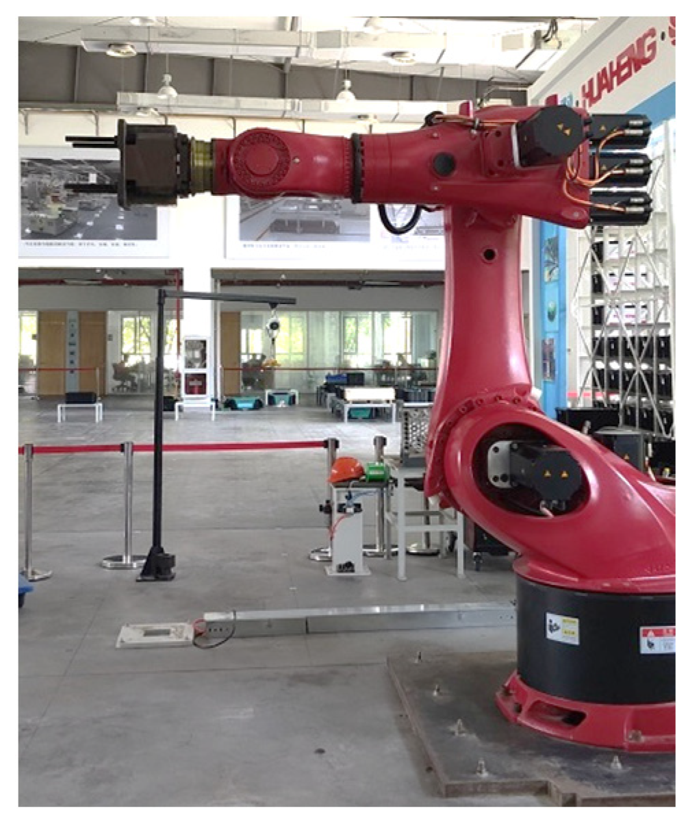
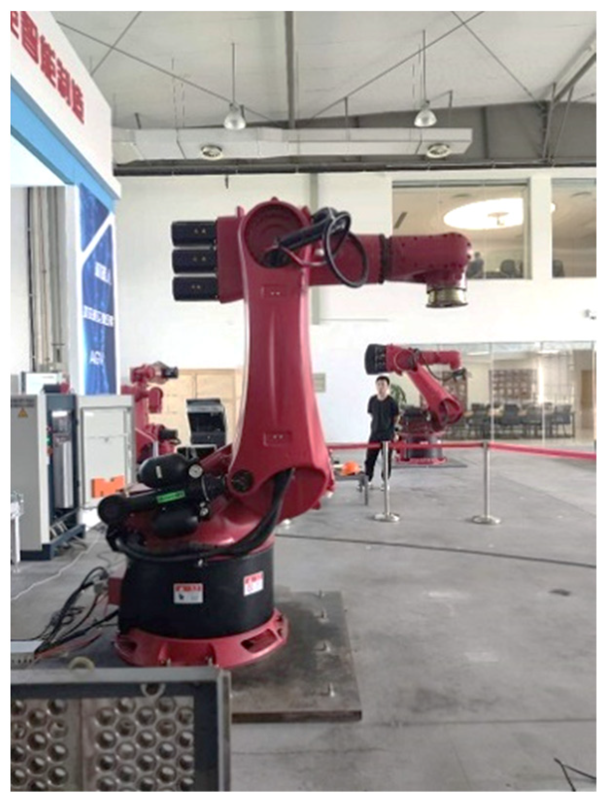
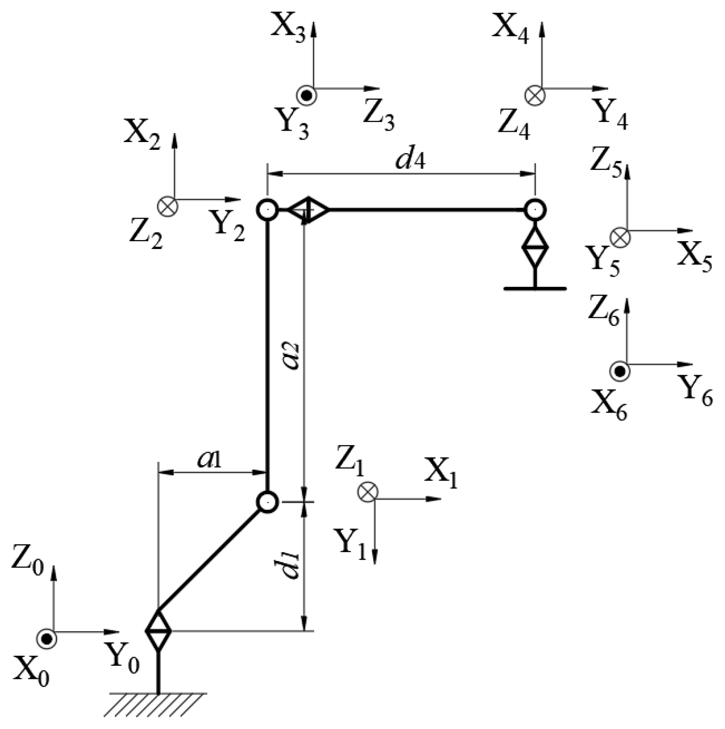
The D-H method is applied to establish the kinematic model of the research object, which is the industrial robot. The D-H parameters of the robot are listed in Table 1. The industrial robot is illustrated in Figure 1, and the coordinate systems of the robot are illustrated in Figure 2.
Regarding the D-H method, there exists a homogeneous transformation matrix, where i represents the number of the coordinate system i :
A i i 1 = [ cos ( θ i ) cos ( α i ) sin ( θ i ) sin ( α i ) sin ( θ i ) a i cos ( θ i ) sin ( θ i ) cos ( α i ) cos ( θ i ) sin ( α i ) cos ( θ i ) a i sin ( θ i ) 0 sin ( α i ) cos ( α i ) d i 0 0 0 1 ]

2.2. Dynamics Model

According to the kinematic model established using the D-H method, recurrence formulas of the dynamics equation based on the Newton–Euler formula are expressed as follows:
Forward recursion: i goes 1 to n ; the angular velocity, angular acceleration, linear acceleration, and enter-of-mass acceleration are calculated by the initial conditions.
Assuming that the base does not move, the initial conditions are as follows:
ω 0 = 0   0   0 T ,   ε 0 = 0   0   0 T ,   g = g x   g y   g z
For the angular velocity:
ω i = R i 1 i ω i 1 + q ˙ i
The angular acceleration can be calculated after Equation (2) is obtained:
R i i 1 = cos q i cos α i sin q i sin α i sin q i sin q i cos α i cos q i sin α i cos q i 0 sin α i cos α i
The linear acceleration can be calculated after Equation (4) is obtained:
p i = a i     d i sin α i     d i cos α i T
a O i = R a O i 1 i 1 i + ε i × p i + ω i × ω i × p i ,
Then, the enter-of-mass acceleration can be obtained by the following equation:
a C i = a O i + ε i × r C i + ω i × ω i × r C i
For the backward recursion: i goes n to 1; forces and torque are calculated from initial conditions.
Assuming there is no external force at the end, the initial condition is as follows:
f n + 1 = τ n + 1 = 0
For the angular velocity:
f i = m i a C i + R i + 1 i f i + 1
The output torque can be calculated after Equation (8) is obtained:
N i = I C i ε i + ω i × I C i ω i
n i = N i + R i + 1 i n i + 1 + p i + r C i × m i a C i + p i × ( R i + 1 i f i + 1 )
τ i = ( R i 1 i z ) T n i
where the meanings of the above symbols are shown in Table 2:

Establishment of Dynamics Model

The establishment of the dynamics model plays a pivotal role in parameter identification. In the systems, analytical solutions can be obtained using the Newton–Euler formula. However, the complexity of the solution increases significantly for the robots with four or more degrees of freedom, which makes it difficult to obtain analytical solutions. To address this challenge, a numerical method is used in this study to establish the dynamics model. Specifically, with the Newton–Euler formulas as the framework, each operation is solved through numerical substitution. This numerical approach is applicable to the joint series robots with any DOF. In comparison to analytical solutions, the higher the degree of freedom (DOF) of the robot, the greater the efficiency of the numerical method relative to the analytical one.
Generally speaking, the Newton–Euler formula is a common form of nonlinear dynamics model in robot dynamics:
M ( q ) q ¨ + C ( q , q ˙ ) q ˙ + g ( q ) = τ
where M q is the inertia matrix in joint space; C ( q , q ˙ ) includes the Coriolis and centrifugal forces, which are nonlinear terms; and g ( q ) is the gravity vector. τ is the joint torque vector. Start by choosing an appropriate operating point. Typically, this is a stable or commonly used posture within the robot’s workspace.
The Newton–Euler model is a nonlinear model with respect to the joint angles, but at the same time a linear model with respect to the parameters. So, the parameters can be decoupled by rearranging the equations. The mathematic results are presented as follows [17]:
τ = Y q , q ˙ , q ¨ P r = Y P r
where Y is the regression matrix, which is a function of q , q ˙ , q ¨ . It represents the nonlinear terms in the dynamics equations. P r represents the parameters vector, which includes the inertial parameters, friction parameters, and other physical parameters of the robot.
Equation (12) is a dynamics model constructed using the Newton–Euler formula, in which the number of columns in the observation matrix Y is identical to that of inertial parameters. The calculation result obtained by using this formula for torque is consistent with that of the backward derivation equation, which means that the inertial parameters P r can be solved by a simpler algorithm.

3. Identification Scheme Design

The robot dynamics model is the basis of parameter identification, and the minimum inertia parameters can greatly simplify the solving process of the robot arm dynamics equation, which is widely used in the robot dynamics model. The minimum inertia parameters usually refer to a set of parameters that can describe the inertia characteristics of the robot joint with a minimum number of parameters. The accurate solution to these parameters is very important for the accuracy of the whole dynamics model.

3.1. Minimum Inertial Parameters

Equation (12) is a linearized form of the dynamics model with respect to the dynamics parameters. With a large number of motion data substituted, it can be found that the observation matrix Y exists in the following form:
Y = y 11 0 y 1 i 0 y 1 × 10 n y 21 0 y 2 i 0 y 2 × 10 n y 31 0 y 3 i 0 y 3 × 10 n y n 1 0 y n i 0 y n × 10 n
The process of solving the parameters is significantly affected by the presence of zero elements in certain columns of the observation matrix, along with linear correlations between columns. To ensure accuracy and robustness, these columns, along with their corresponding inertial parameters, must be discounted. Through this refinement, it is ensured that only relevant and independent data contribute to identification. Thus, the efficiency and effectiveness of the process are enhanced.
If the columns containing zero elements comprise m 1 columns and linear correlation results in the removal of m 2 columns, the observation matrix is downsized accordingly. Therefore, the new size of the observation matrix is obtained as n 10 n m 1 m 2 , where n represents the number of rows in the matrix.
A method for obtaining minimum inertial parameters is described in the symPybotics toolkit based on Python 3.2 [18]. The method is based on QR decomposition, and the obtained result contains only the symbol expression of the inertia parameters, which can be used in this research. With the minimum inertial parameters obtained, a new dynamics model is developed as follows:
τ = Y m P m r
where Y m and P m r represent the observation matrix and inertial parameters sets, respectively, in the form of their minimum inertia parameters.

3.2. Friction Force Model

The friction in robots occurs primarily in rotating joints, which has a significant impact on the experimental results. In terms of robot control, the main factors to consider for friction include Coulomb friction and viscous friction, as the frictional effects can be adequately addressed [19]. The Coulomb–viscous friction model is expressed as follows:
τ f i = s i g n q ˙ i k i 1 + q ˙ i k i 2 τ f = τ f 1 τ f 2 τ f n T
where τ f i is the friction moment of No. i joint, k i 1 is the Coulomb friction coefficient of No. i joint, k i 2 is the viscosity friction coefficient of No. i joint, and s i g n x is a symbolic function.
In the identification with friction force, the friction force will produce extra torque when the robot is moving, and this torque needs to be overcome by the robot joint drive. So, in the calculation, the friction torque is a component of the total torque. After adding it to the dynamics model, the new dynamics model can be expressed as follows:
τ = Y m P m r + τ f
The coefficient of friction can be obtained at the same time through the identification of robot dynamics parameters, and the joint torque can be solved through the inverse dynamics calculation based on this model.

3.3. Parameters Identification System

If the kinematic model is known, the kinematic parameters can be solved using the parameter identification Equation (17) as obtained by the least square method.
P ^ m f r = Y S T Y S 1 Y S T Γ
where P ^ m f r is the inertial parameters sets including friction object.
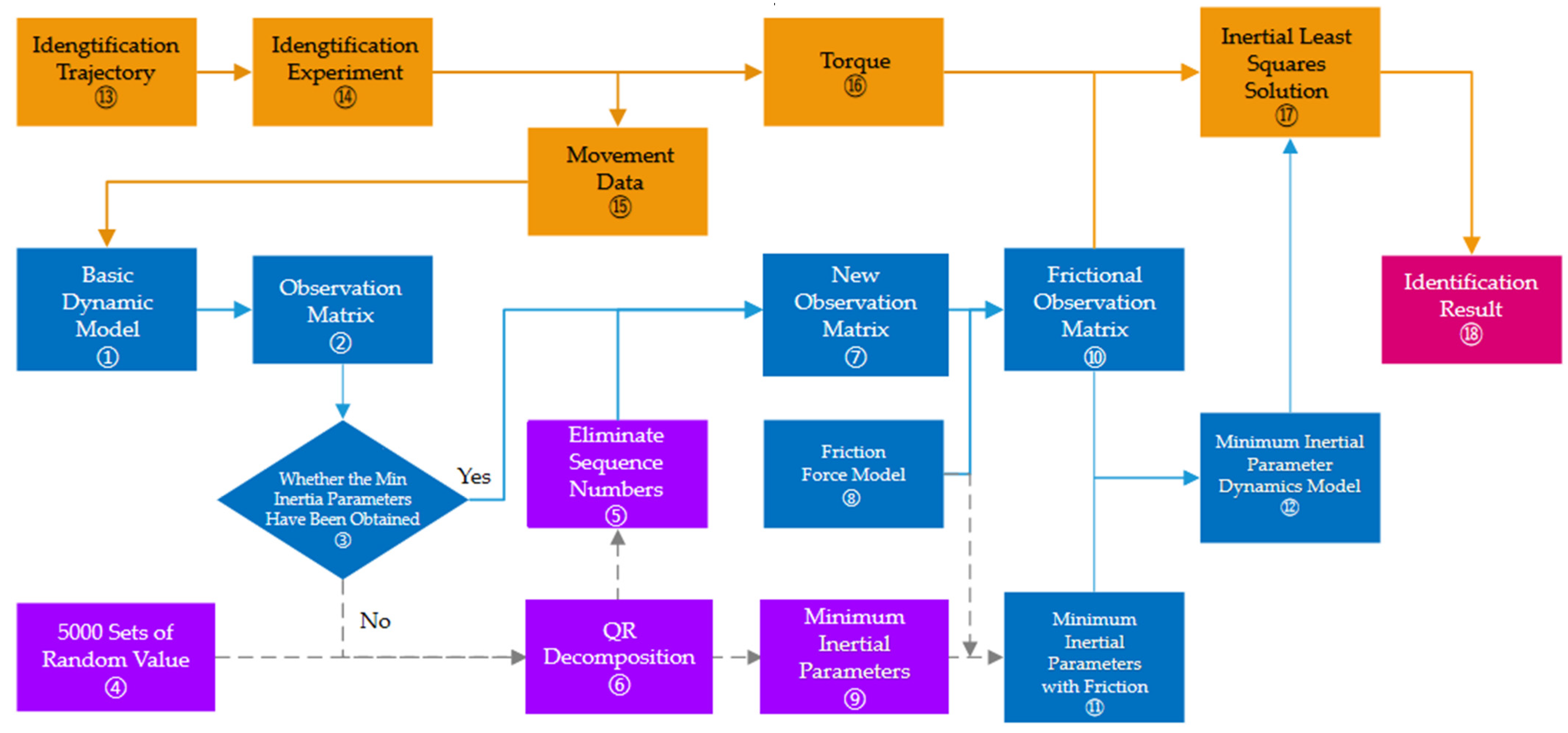
According to Equation (17) and the contents described in the previous parts, the whole parameter identification process and system can be summarized. The system includes three steps: the dynamics model, solution to the inverse dynamics problem, and identification of minimum inertia parameters.
For the sake of illustration, Figure 3 illustrates the dynamics parameter identification system developed for a robot with multiple DOF, which is based on a previous summary of the theoretical basis and identification process.
Figure 3 illustrates the dynamics parameter identification system developed for a robot with multiple DOF, highlighting three main pathways:
Pathway 1 (Steps ① to ⑪): This pathway aims to obtain a preliminary dynamics model of the minimum inertial parameters. It starts from the basic dynamics model, and a simplified dynamics model with friction force objects is obtained through mathematical transformation. The simplified model includes only minimum internal parameters, which lays a foundation for the subsequent dynamics analysis. In this pathway, QR decomposition is used for obtaining the minimum internal parameters. Furthermore, the Coulomb friction model is also added and discussed.
Pathway 2 (Steps ① to ③, ⑦, ⑧, and ⑩ to ⑫): The pathway is used to solve the inverse dynamics of the robot, which involves various steps. Its main goal is to calculate the torque and force required by the robot joint to achieve the desired motion trajectory through the inverse kinematic equations. This part is the core of this system.
Pathway 3 (Steps ⑬ to ⑮, ① to ③, ⑦, ⑧, ⑩, and ⑯ to ⑱): This pathway, which involves orange blocks, is dedicated to identifying the minimum inertial parameters. It intersects with the blue block pathway at certain steps. In general, the motion data of the robot arm obtained through identification experiments in this path need to be input into pathway 2, through which the output dynamics model includes only the minimum inertia parameters; the final identification parameters are obtained by the least square method.
According to the parameters identification system, the description of the steps and process is shown in Table 3.

4. Incentive Trajectory Planning

For the identification of robot dynamics parameters, the periodic finite Fourier series is commonly adopted for the excitation trajectory of the experiment [20], as described in Equations (18)–(20). Because of the periodicity of the Fourier series, the robot can improve the signal-to-noise ratio by means of multiple sampling to obtain ideal data. Through the periodic nature of the trajectory, each joint can return to its initial position simultaneously after a cycle of movement is complete. By operating the robot through multiple cycles, any inherent random errors can be reduced by averaging multiple samples. Thus, experimental data of greater accuracy can be obtained
q i t = l = 1 N a l i ω f l sin ω f l t b l i ω f l cos ω f l t + q i 0
q ˙ i t = l = 1 N a l i cos ω f l t + b l i sin ω f l t
q ¨ i t = l = 1 N a l i ω f l sin ω f l t + b l i ω f l cos ω f l t
where q i t is the displacement of the No. i link as a function of time, N is the number of harmonics considered in the Fourier series, and a l i , b l i , q i 0 are the coefficients to be optimized. More precisely, a l i and b l i are the sine and cosine coefficients of the No. l harmonic component for the No. i link. These coefficients determine the contribution of each harmonic to the total displacement, and ω f is the base frequency of the Fourier series. w f l is the angular frequency of the No. l harmonic, which can determine the frequency of each harmonic.
q t 0 = q t f = 0 q ˙ t 0 = q ˙ t f = 0 q s min q t q s max q ˙ t | q ˙ | max q ¨ t | q ¨ | max
Equation (21) represents the boundary condition for trajectory planning. Table 2 lists the joint design parameters, including the angle limit, rated angular velocity, and maximum angular acceleration. The angle limit is defined as the increment in the zero position of the robot, as shown in Table 4.
The base frequency of the Fourier series ω f is 0.1 Hz, and the running time of the trajectory is 10 s. In Equations (18)–(20) above, N = 5 is taken, that is, the fifth-order Fourier series is adopted. The main problem in obtaining the optimal trajectory is to find the coefficients in Equation (18). Each joint contains 11 coefficients, and there are 66 unknown parameters to be solved. In the case of multiple coefficients, a genetic algorithm can be used to solve them.
If the population size is set to 100 and there are 66 random parameters in one individual, there will be 6600 parameters in one generation. At the same time, the binary coding method is adopted. The number of conditions of the observation matrix is taken as the optimization index. The formula for calculating the condition number is as follows:
cond ( Y ) = Y Y 1
where Y is the norm of matrix.
The condition number is usually used to describe the stability of a linear system. The smaller the condition number, the better the stability of the system and the smaller the error of the solution.
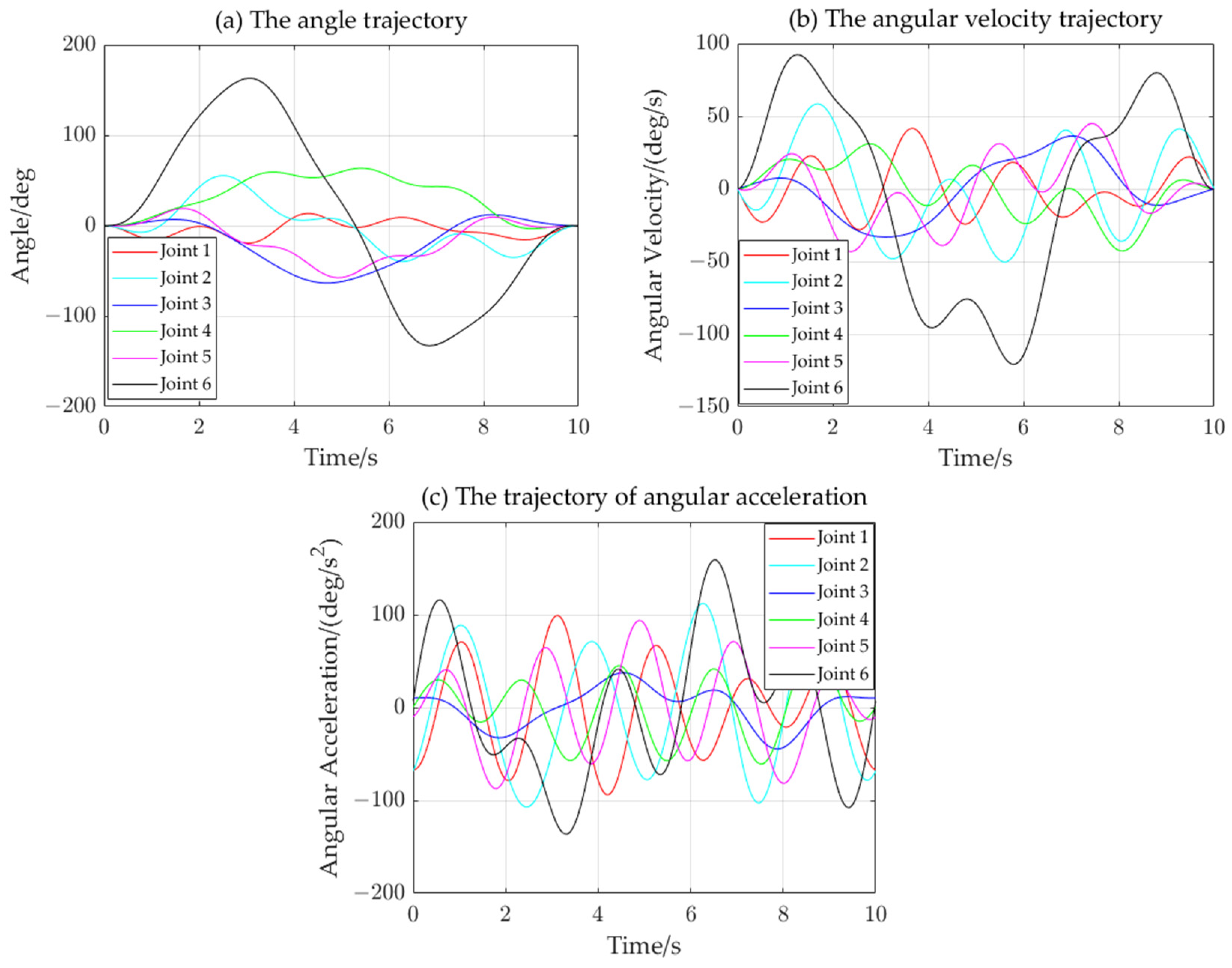
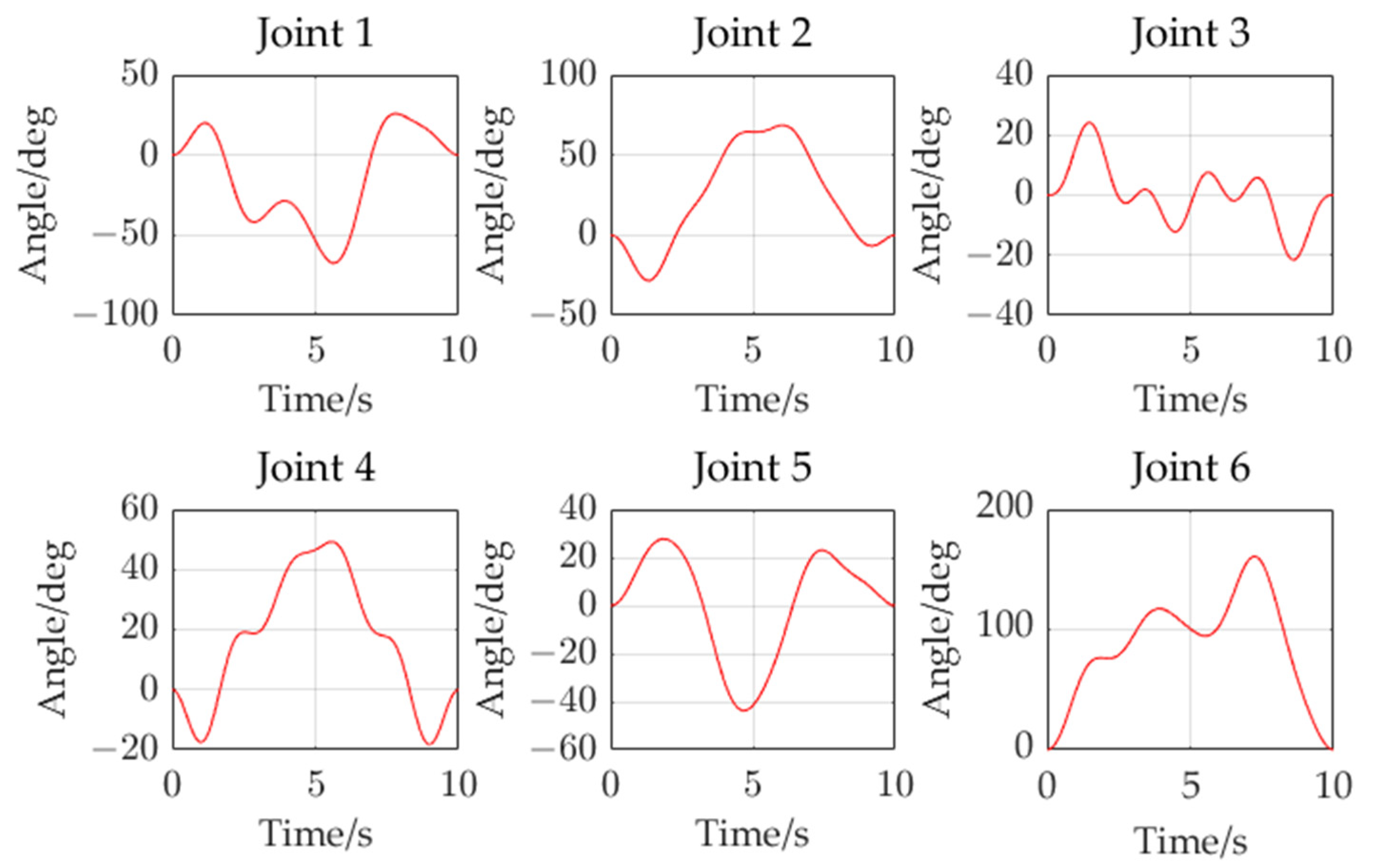
MATLAB R2020b was used to solve genetic algorithm and output the results. After the end of the solution, the angle at the zero moment sometimes has a small zero shift, and q i 0 in the coefficient can directly affect the zero position. The adjustment of q i 0 according to this offset can make the angle at the zero moment closer to zero. The results are shown in Figure 4.

5. Simulation and Experiment

5.1. Parameters Identification Simulation

Simulation is required for comprehensive application and verification of the theoretical framework. The parameter identification system can be theoretically validated through simulation, which provides a significant reference for conducting field experiments.
Dynamics simulation was performed using Adams 2020. In an Adams simulation, each coordinate system relates to each link. Finally, it should be noted that in an Adams simulation, the centroid coordinates and inertia tensors need to be modified relative to the link coordinate system, and all values should be consistent with those given in the MATLAB dynamics model. At the same time, the position of the centroid coordinates is also relative to the link coordinate system. The robot model consists only of rotating joints and joint rotation drives, and the base is fixed to the ground.
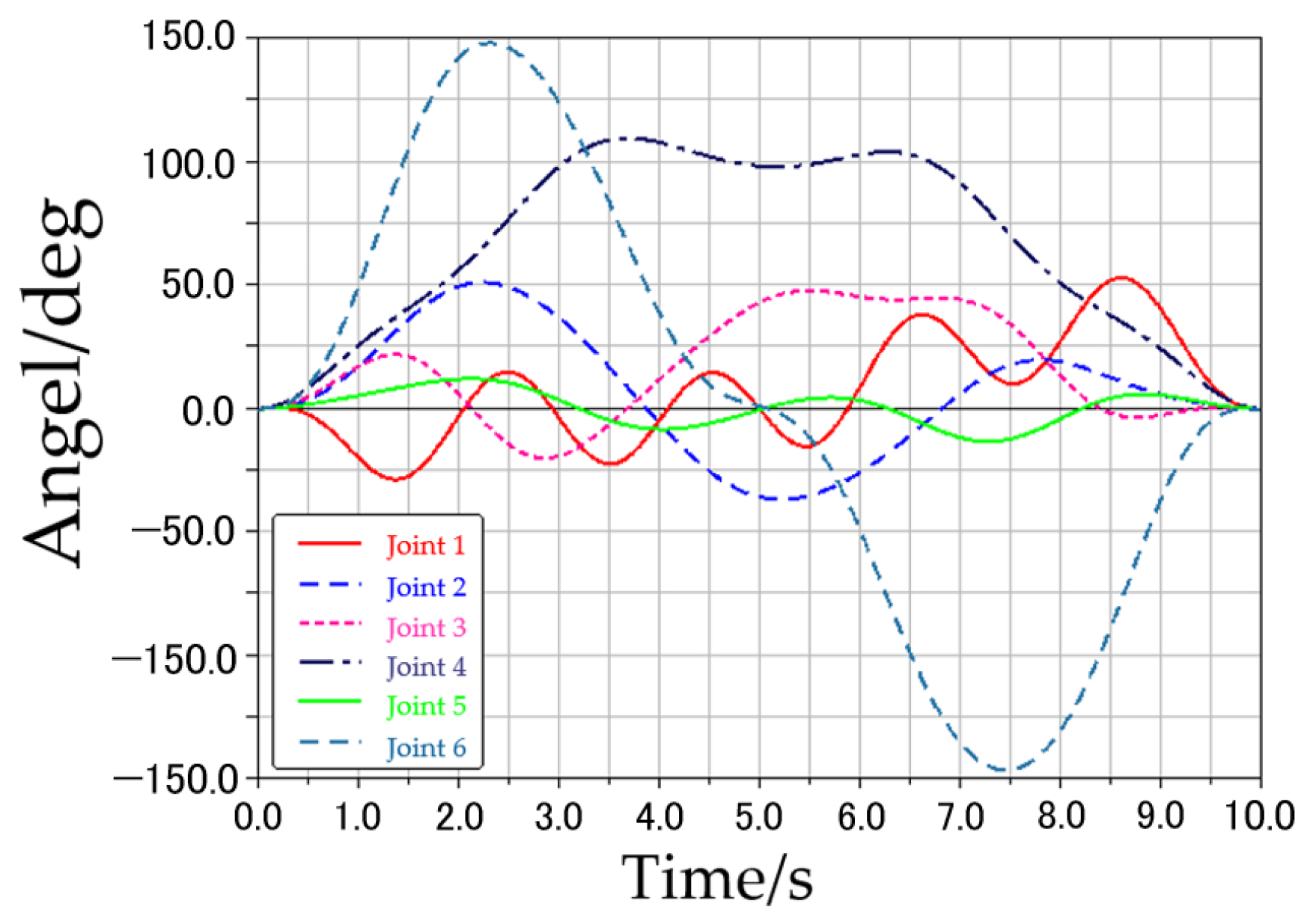
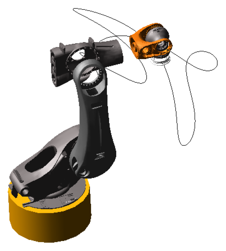
In order to verify the accuracy and universality of the calibration method, another trajectory was selected for simulation. Figure 5 shows the input of angle values in Adams, while Figure 6 illustrates the spatial trajectory obtained through simulation. Regarding the control strategy for the robot, the joint angle control strategy is used, which refers to the direct control of the rotation angles to ensure that the robot’s joints move along a predetermined trajectory.
In the simulation, the robot moves continuously for several periods according to the planned trajectory. The average value of identification results is obtained through multiple simulations. The parameters identification system proposed in this study is adopted to carry out the identification process, which ignores friction force. The results of parameter identification are obtained, as shown in Table 5, where Δ P is the absolute value of the difference between the theoretical and simulated values.
As shown in Table 5, only five parameters have a difference between theory and practice. Among them, except for the error of the fourth parameter, the error of the remaining four parameters is less than 0.1% of the actual value, which is in the allowable range of error. The results verify that the theory behind the identification system is correct.

5.2. Experimental Procedure

The experiment was conducted using the industrial robot system. The robot used the LAFERT B1028I-04208 servo motor as the power producer and the servo motor built-in encoder for coding, and the NI software system was used for control with the NI controller cRIO-9055. To accurately track and position the robotic arm, an API laser tracker, specifically API-T3, was used, which can achieve an accuracy of 0.01 mm.
A unified identification method was applied, where the robot joints move simultaneously along a planned trajectory of continuous movement for several cycles. The data were collected and processed accordingly. Finally, the least squares method was used to estimate the dynamics parameters.
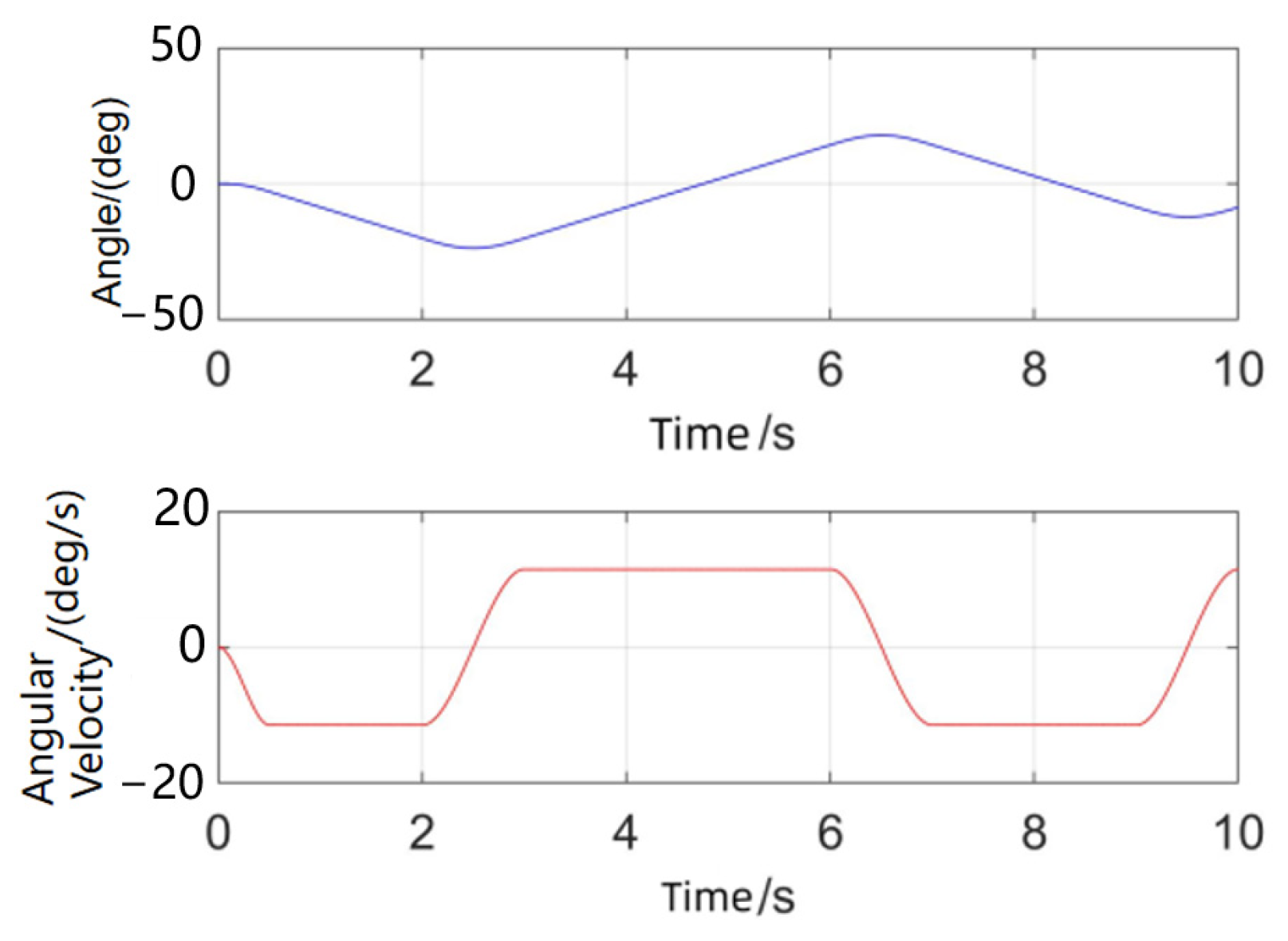
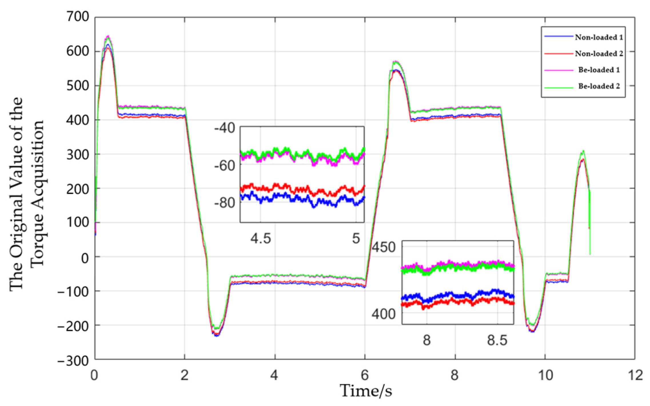
The torque values obtained from the motor driver during the experiment are the motor torque coefficients listed in Table 6, determined using the software of the motor driver. These coefficients were used to convert the obtained values into real torque. To ensure the accuracy of the coefficients, on-site verification was necessary. To calibrate the motor torque coefficient for joint 3, the real torque was first obtained under both no-load and load conditions. Then, the theoretical torque was calculated by converting the collected drive data using the motor torque coefficient and deceleration ratio. Finally, the theoretical torque was compared with the real torque. To initiate the calibration process, joint 5 was rotated from the vertical state to the horizontal one, aligning joints 6 and 4 horizontally, as shown in Figure 7, representing the no-load state. The load comprised a counterweight and connecting parts, totaling 15.5 kg, as illustrated in Figure 8. It was mounted at the end of the robot. The distance between the center of mass and the axis of joint 3 was determined as 1.405 m, with a torque of 213.42 N·m.
When connecting rod 3 reaches a horizontal position, the torque exerted by the load on joint 3 equals the one generated by the gravitation of the load. The trajectory of the angle and angular velocity are depicted in Figure 9.
During this process, the horizontal position was passed twice during one cycle. Additionally, both the no-load and load conditions were operated for two cycles each to ensure comprehensiveness in data collection and analysis.
Figure 10 illustrates the dimensionless torque values obtained. Specifically, at the horizontal position of joint 3, the corresponding time instances are recorded at 4.75 s and 8.25 s. To ensure accuracy, an average duration of 50 ms is considered before and after these time points. Subsequently, the data obtained from “no load 1” and “no load 2”, respectively, are subtracted from the averaged results of “load 1”. The same procedure was followed to produce eight distinct results Δ T ¯ 1 ~ Δ T ¯ 8 for “load 2”, as detailed in Table 7.
The average of the data shown in Table 7 was found to be 22.69. With this value multiplied by the torque constant and the deceleration ratio of joint 3, which is shown in Table 5, theoretical torque was obtained as 209.96 N·m, which represents the force of the load on the joint. This value is comparable to the actual value of 213.42 N·m, which is calculated in the field calculation mentioned above. The result demonstrates the accuracy of the motor torque coefficient.
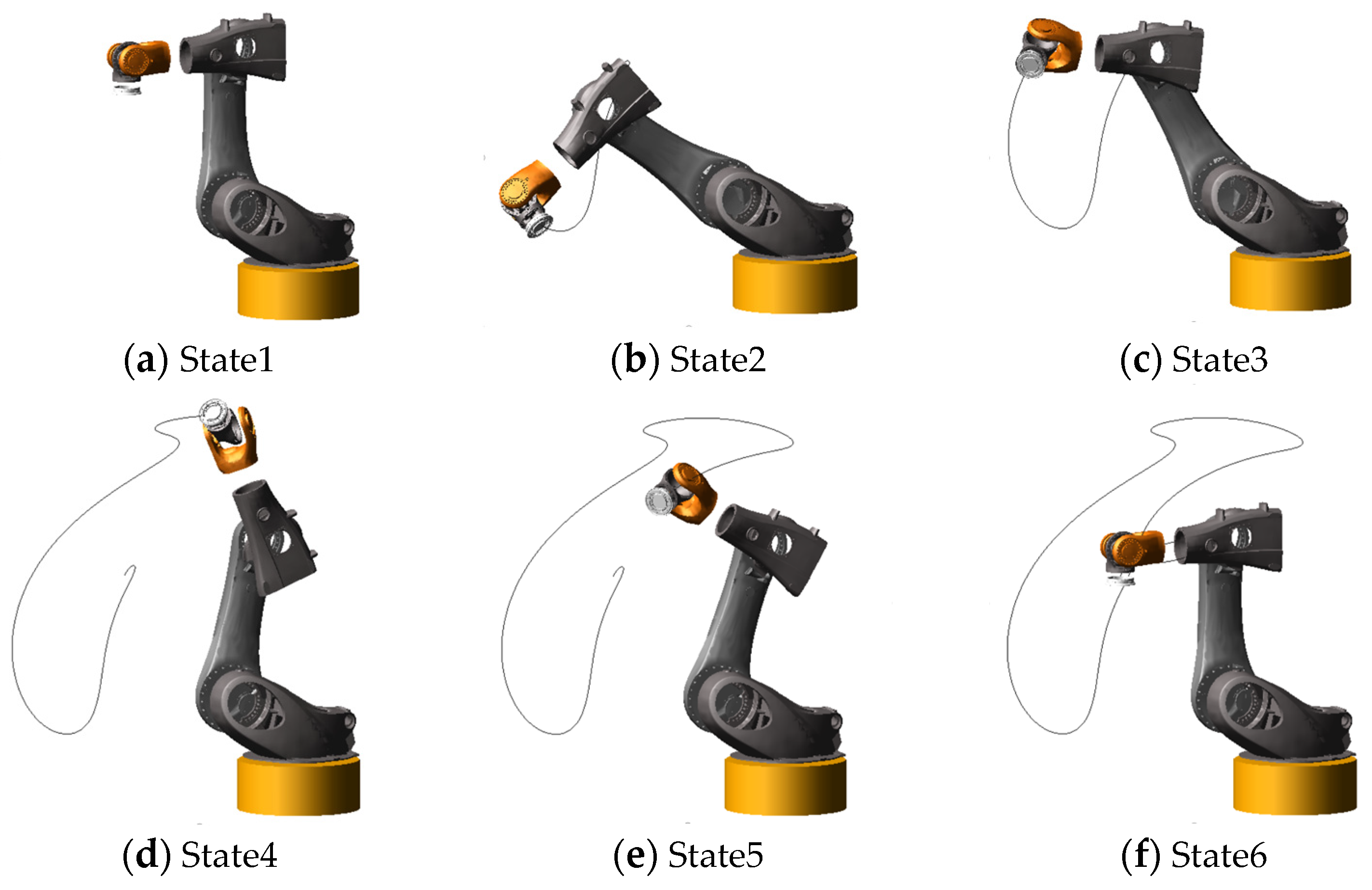
In the experiment, the trajectory illustrated in Figure 4 was adopted. To ensure safety during the experiment, Adams was applied to simulate the trajectory in advance. The simulation trajectory is shown in Figure 11, from which any potential robot interference or collisions can be observed.
Adams visual trajectory was observed, which ensures that the robot is operated safely. In general, it is difficult to input the point position of the trajectory directly into the program of the upper computer. Instead, the data of position need to be multiplied by the corresponding encoder transmission ratio. This is because the final response of the robot would be very weak if the planned angle value were directly inputted. The transmission ratio of encoders at each joint is listed in Table 8.
Each operation proceeded for three cycles. Thus, the angular trajectory is discretized into 30,001 points, given a pulse control interval of 1 ms and a trajectory period of 10 s.
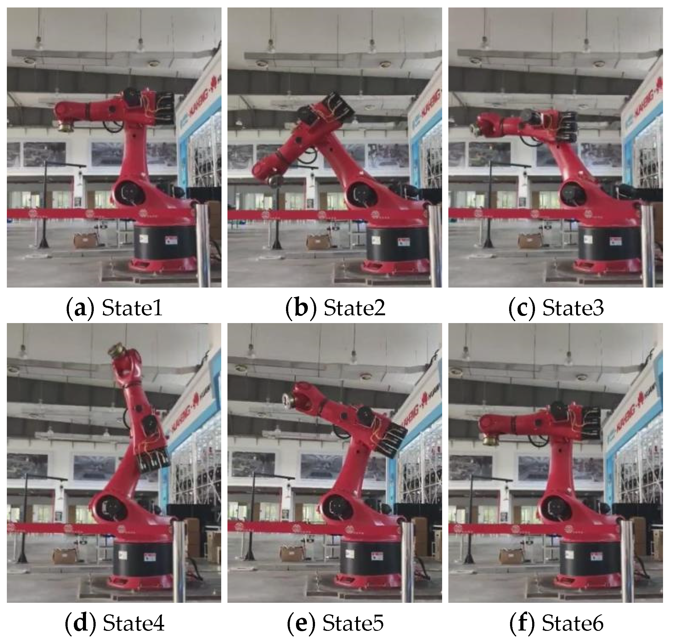
The process of operating the robot is shown in Figure 12. Its trajectory is completely consistent with that in Figure 11, indicating that the input is accurate.

5.3. Experimental Data Processing and Analysis

Angle and angular velocity data are subject to averaging and smoothing filtering, which leads to results that are consistent with those shown in Figure 4a,b.
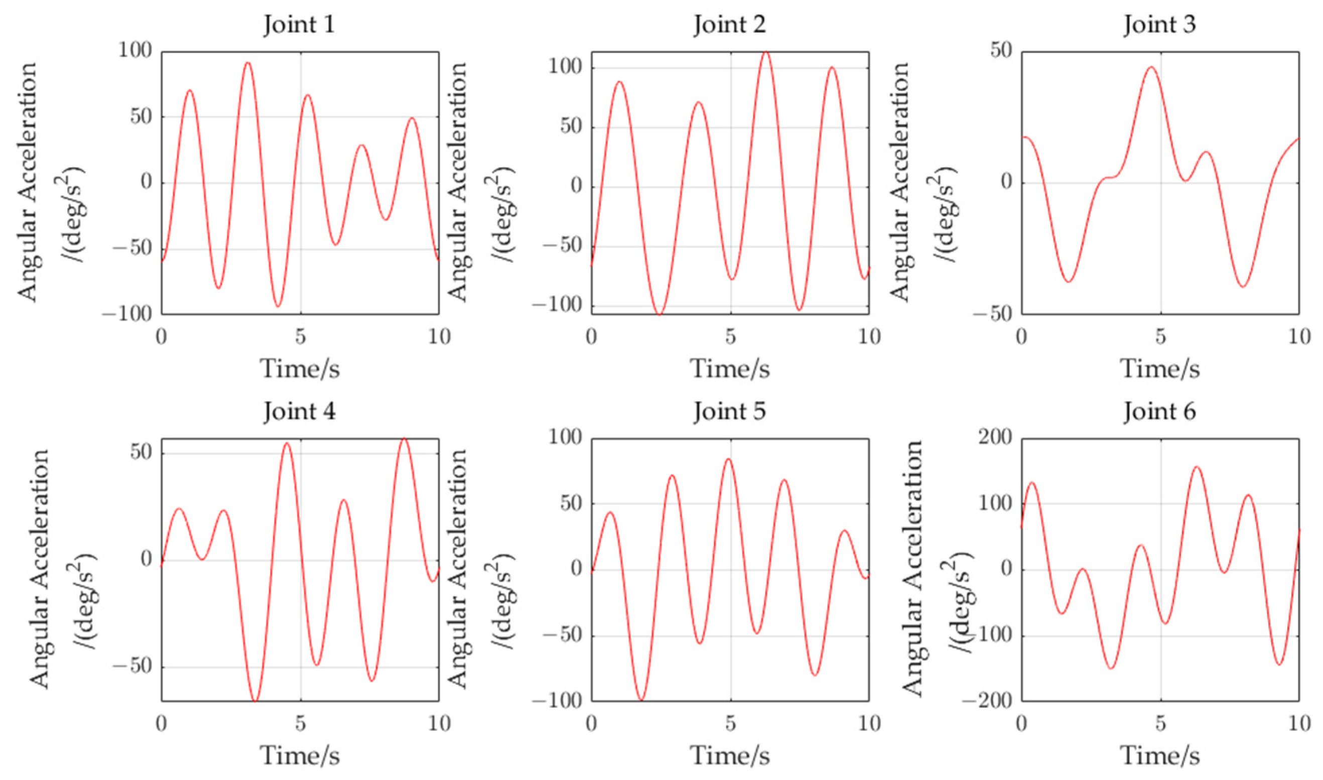
Since joint acceleration cannot be obtained directly, it is determined through the trajectory of motion, which is a continuous function. Through numerical calculation, acceleration can be determined by applying a difference algorithm to known angular velocity data.
In numerical differentiation, the sampling interval h is used to facilitate the derivative calculation of discrete functions [21].
f x = f x + h f x h 2 h + O h 2
By ignoring error O h 2 , the following is obtained:
f x f x + h f x h 2 h
Based on Equation (15), the joint angular acceleration is obtained by using angular velocity, as shown in Figure 13.
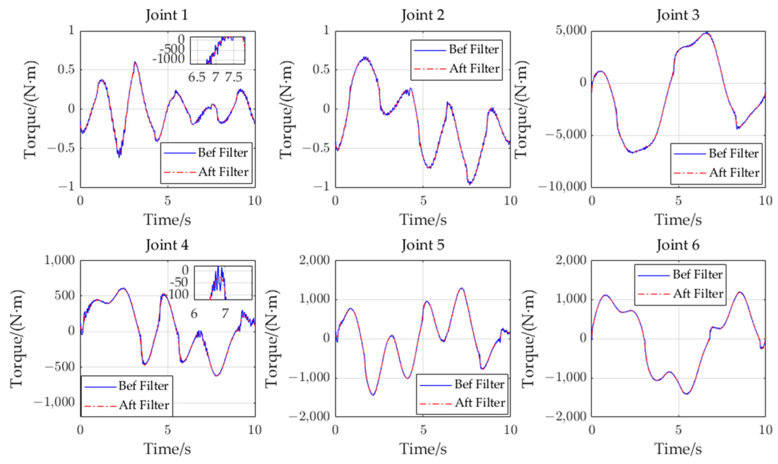
The torque was averaged and filtered. Figure 14 shows the comparison of results obtained before and after filtering.

5.4. Obtaining Minimum Inertial Parameters

By substituting the motion data into the dynamics model of parameter identification, the observation matrix can be obtained. The minimum inertial parameter set of the robot was obtained, as listed in Table 9.
According to the results in Table 9, a total of 48 minimum inertial parameters were obtained, among which the first 36 are the original minimum inertial parameters, and the last 12 are the coefficients of friction. These values are the dynamics parameters of the robot, which can be used for inverse dynamics operations.

6. Experimental Verification

After solving for the minimum inertial parameters, two methods of self-trajectory verification and general trajectory verification were adopted.
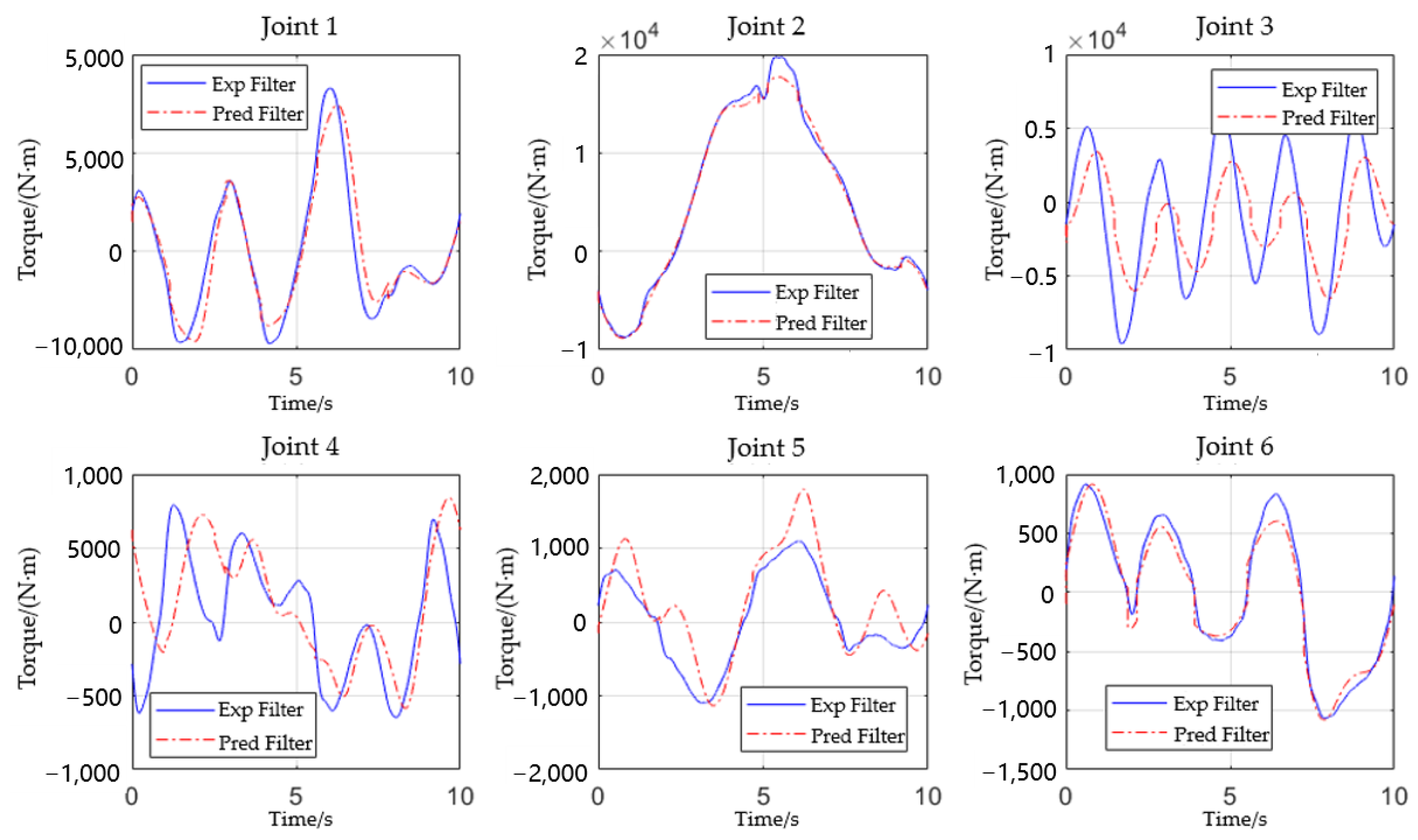
(1) Self-trajectory verification: The minimum inertial parameters identified by a set of trajectories were taken as new dynamics parameters and substituted into the dynamics model as the minimum inertial parameters. Subsequently, the angle, angular velocity, and angular acceleration of the trajectories were inputted to solve the theoretical torque, which is also known as the predicted torque. The prediction results were compared with the experimental results, as shown in Figure 15.
According to the comparison results shown in Figure 15, the predicted torque of joints 1, 2, and 6 are consistent with the experimental torque. Although the predicted torque of joints 3, 4, and 5 exhibit a significant local deviation from the experimental torque, the trend of torque prediction is consistent.
(2) General trajectory verification: Parameter identification is purposed mainly to ensure the identified inertial parameters are applicable in all trajectory scenarios and can be used to predict joint output torque under different conditions. To achieve this purpose, the inertial parameters identified in the experiment were taken as known quantities to forecast the output torque given a different set of trajectories. This predicted torque was then compared with the experimental torque to evaluate the experimental results.
An alternative set of trajectories, as illustrated in Figure 16, was used for this purpose. Adams software was applied to demonstrate the motion envelope of these trajectories in a safe way. Subsequently, the trajectories were inputted into the robot control system, with data collected on angle, angular velocity, angular acceleration, and experimental torque. The data on angle, angular velocity, and angular acceleration were inputted into the dynamics model containing the identified inertial parameters for calculation of the predicted torque. Finally, the experimental torque was compared with the predicted torque, as shown in Figure 17.
As shown in Figure 17, the overall effect of torque prediction for joint 1, 2, and 6 is satisfactory and comparable to the experimental torque. The torque trends of joint 3, 4, and 5 are similar, but the amplitude error is significant. Overall, this method plays a certain role in the identification of robot dynamics parameters, despite some persistent errors that need to be analyzed according to the phenomena occurring in the experiment.
In the process of experimental verification, the outcomes of identification performed using the two verification methods were found to be unsatisfactory. Therefore, tentative analysis was performed to determine the causes of the above errors:
(1)
Coupling of joint drive structure:
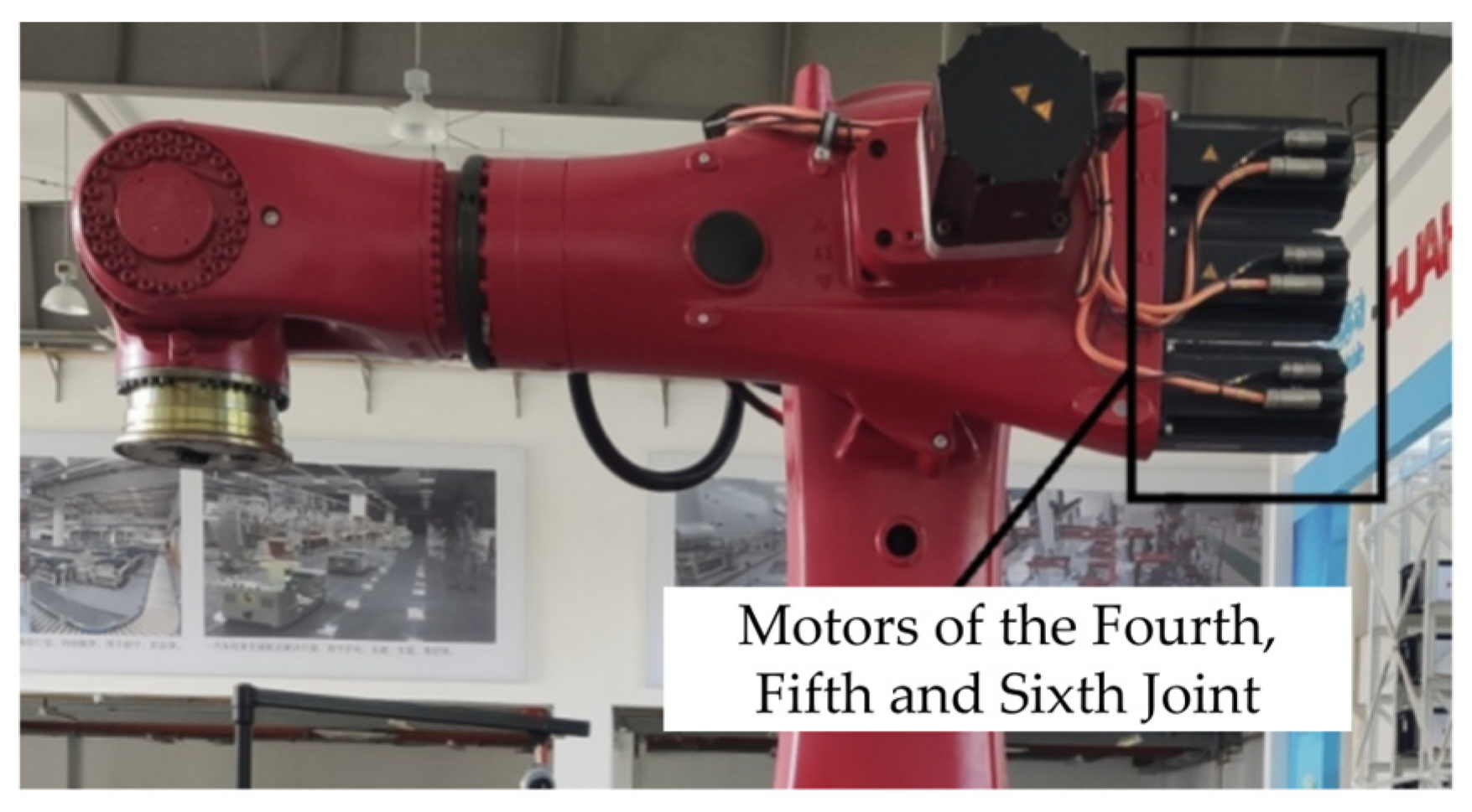
In the process of deduction and simulation, each connecting rod is assumed to be an independent model and the satisfactory outcome of identification is produced. However, in the experimental robot, the motors of the back three joints are all positioned at the first end of connecting rod 3, as shown in Figure 18. The torque is transmitted to joints 4, 5, and 6 through the transmission mechanism. As the identified objects are not independent linkages, the dynamics model is not as accurate as required.
(2)
Torque acquisition is inaccurate:
The torque value is obtained directly by the motor driver, and the calculation is based on the current. However, when the robot is operated at variable acceleration and high speeds, the current of the driver fluctuates significantly, which causes random errors in the obtained values. By introducing an external torque sensor, the accuracy of torque acquisition can be enhanced, thus mitigating the impact of fluctuations and improving the overall quality of the data.

7. Conclusions

This paper primarily develops a system for dynamics parameter identification in robots. By establishing and verifying a robot dynamics model, combining the minimum inertia parameter set and friction model, the inertial parameters of the robot are accurately identified by least square method, genetic algorithm, and Fourier series. By making a comparative analysis of simulation and experiment results, the following is concluded:
  • Through simulation experiments, the validity of the model was verified. The simulation results showed that the predicted dynamics response was highly consistent with the experimental data, which proves the accuracy of the simulation model and the theoretical model;
  • In the identification experiment phase, 48 minimum inertia parameters were successfully identified, including joint parameters and friction parameters. Self-trajectory verification showed that the predicted torques of joints 1, 2, and 6 were consistent with the experimental data;
  • In the experimental verification stage, two verification methods were adopted. The results show that the predicted torque was consistent with the experimental torque in the trend, and the inertia parameters were generally used under different trajectory conditions.
However, there are limitations to this study. The inaccurate torque acquisition and the coupling of the robot joint structure cause slight errors. In the future, the model can be improved to more accurately reflect the coupling effect of the robot, and the applicability of the method to other types of robots and application scenarios can be explored. The system can be applied to most 6-DOF rotary joint robots with high precision, low cost, and fast calculation speed, and can be used in high-torque application scenarios. It can be applied to industrial practice and provides valuable insights for practical engineering applications

Author Contributions

Conceptualization, Q.Y. and Z.Y.; methodology, Z.Y. and Q.Y.; software, Z.Y. and Q.Y.; writing—Z.Y. and K.Z.; writing—review and editing, Z.Y. and Y.Q.; supervision, Z.Y. and Y.Q. All authors have read and agreed to the published version of the manuscript.

Funding

This research received no external funding.

Data Availability Statement

Due to privacy or ethical constraints, the data require contacting the author for access.

Conflicts of Interest

The authors declare no conflicts of interest.

References

  1. Gautier, M.; Khalil, W. A Direct Determination of Minimum Inertial Parameters of Robots. In Proceedings of the 1988 IEEE International Conference on Robotics and Automation, Philadelphia, PA, USA, 24–29 April 1988; pp. 1682–1687. [Google Scholar]
  2. Gautier, M.; Khalil, W. Direct calculation of minimum set of inertial parameters of serial robots. IEEE Trans. Robot. Autom. 1990, 6, 368–373. [Google Scholar] [CrossRef]
  3. Qin, Z.; Baron, R.; Birglen, R. A New Approach to the Dynamic Parameter Identification of Robotic Manipulators. Robotica 2010, 28, 539–547. [Google Scholar] [CrossRef]
  4. Yang, J.; Harsono, E.; Yu, H. Dynamic modeling and validation of a hybrid-driven continuum robot with antagonistic mechanisms. Mech. Mach. Theory 2024, 197, 105635. [Google Scholar] [CrossRef]
  5. Franceschi, P.; Pedrocchi, N.; Beschi, M. Identification of human control law during physical Human–Robot Interaction. Mechatronics 2023, 92, 102986. [Google Scholar] [CrossRef]
  6. Harandi, M.R.J.; Hassani, A.; Hosseini, M.I.; Taghirad, H.D. Adaptive Position Feedback Control of Parallel Robots in the Presence of Kinematics and Dynamics Uncertainties. IEEE Trans. Autom. Sci. Eng. 2024, 21, 989–999. [Google Scholar] [CrossRef]
  7. Huang, Y.; Ke, J.; Zhang, X.; Ota, J. Dynamic Parameter Identification of Serial Robots Using a Hybrid Approach. IEEE Trans. Robot. 2023, 39, 1607–1621. [Google Scholar] [CrossRef]
  8. Robet, P.; Gautier, M.; Jubien, A.; Janot, A. A new output error method for a decoupled identification of electrical and mechanical dynamic parameters of DC motor-driven robots. IFAC Proc. Vol. 2012, 45, 25–30. [Google Scholar] [CrossRef]
  9. Roveda, L.; Forgione, M.; Piga, D. Robot control parameters auto-tuning in trajectory tracking applications. Control Eng. Pract. 2020, 101, 104488. [Google Scholar] [CrossRef]
  10. Taghbalout, M.; Antoine, J.F.; Abba, G. Experimental Dynamic Identification of a YuMi Collaborative Robot. IFAC-PapersOnLine 2019, 52, 1168–1173. [Google Scholar] [CrossRef]
  11. Perrusquía, A.; Garrido, R.; Yu, W. Stable robot manipulator parameter identification: A closed-loop input error approach. Automatica 2022, 141, 110294. [Google Scholar] [CrossRef]
  12. Aivaliotis, P.; Papalitsa, E.; Michalos, G.; Makris, S. Identification of dynamic robot’s parameters using physics-based simulation models for improving accuracy. Procedia CIRP 2021, 96, 254–259. [Google Scholar] [CrossRef]
  13. Han, Y.; Wu, J.; Liu, C.; Xiong, Z. An Iterative Approach for Accurate Dynamic Model Identification of Industrial Robots. IEEE Trans. Robot. 2020, 36, 1577–1594. [Google Scholar] [CrossRef]
  14. Siwek, M.; Panasiuk, J.; Baranowski, L.; Kaczmarek, W.; Prusaczyk, P.; Borys, S. Identification of Differential Drive Robot Dynamic Model Parameters. Materials 2023, 16, 683. [Google Scholar] [CrossRef] [PubMed]
  15. Tadese, M.A.; Yumbla, F.; Pico, N.; Moon, H. Application of A Reliable Dynamic Friction Model for Accurate Dynamic Model Parameters Estimation of Robot Manipulators. In Proceedings of the 2022 22nd International Conference on Control, Automation and Systems (ICCAS), Jeju, Republic of Korea, 27 November–1 December 2022; pp. 1916–1923. [Google Scholar]
  16. Lomakin, A.; Deutscher, J. Identification of Dynamic Parameters for Rigid Robots based on Polynomial Approximation. In Proceedings of the 2020 IEEE/RSJ International Conference on Intelligent Robots and Systems (IROS), Las Vegas, NV, USA, 24 October 2020–24 January 2021; pp. 7271–7278. [Google Scholar]
  17. Huo, W. Robot Dynamics and Control; Higher Education Press: Beijing, China, 2005; pp. 100–102. [Google Scholar]
  18. Xu, C. Research on Dynamic Parameter Identification and Feed forward Control of Articulated Robots. Ph.D. Dissertation, Southeast University, Nanjing, China, 2017. [Google Scholar]
  19. van Duijkeren, N.; Verschueren, R.; Pipeleers, G.; Diehl, M.; Swevers, J. Path-following NMPC for Serial-link Robot Manipulators Using a Path-parametric System Reformulation. European Control Conference. In Proceedings of the 2016 European Control Conference (ECC), Aalborg, Denmark, 29 June–1 July 2016; pp. 477–482. [Google Scholar]
  20. Reynoso-Mora, P.; Chen, W.; Tomizuka, M. A convex relaxation for the time-optimal trajectory planning of robotic manipulators along predetermined geometric paths. Optim. Control Appl. Methods 2016, 37, 1263–1281. [Google Scholar] [CrossRef]
  21. Sun, Z.; Yuan, W.; Wen, Z. Numerical Analysis, 3rd ed.; Southeast University Press: Nanjing, China, 1993; pp. 321–326. [Google Scholar]
Figure 1. Industrial robot.
Machines 12 00595 g001
Figure 2. Robot coordinate systems.
Machines 12 00595 g002
Figure 3. Robot kinematics parameter identification system.
Machines 12 00595 g003
Figure 4. Fourier series trajectories.
Machines 12 00595 g004
Figure 5. Angle change curves of joints 1 to 6 in Adams.
Machines 12 00595 g005
Figure 6. Spatial motion trajectory.
Machines 12 00595 g006
Figure 7. No load at the end of the robot.
Machines 12 00595 g007
Figure 8. With a load at the end of the robot.
Machines 12 00595 g008
Figure 9. Angle and angular velocity of joint 3.
Machines 12 00595 g009
Figure 10. Verification of torque coefficient of joint 3.
Machines 12 00595 g010
Figure 11. Theoretical Spatial Trajectory.
Machines 12 00595 g011
Figure 12. Space trajectory field experiment.
Machines 12 00595 g012
Figure 13. Angular accelerations of each joint.
Machines 12 00595 g013
Figure 14. Comparison of torque before and after filtering.
Machines 12 00595 g014
Figure 15. Comparison of the experimental and prediction values of torque for the self-trajectory.
Machines 12 00595 g015
Figure 16. Angle change curves of the general trajectory.
Machines 12 00595 g016
Figure 17. Comparison of the theoretical and simulated values of torque for the general trajectory.
Machines 12 00595 g017
Figure 18. Position of the rear three-joint motor.
Machines 12 00595 g018
Table 1. D-H parameters of the industrial robot.
Link Number i a i /mm α i /rad d i /mm θ i /rad
1350 π / 2 684 θ 1 π / 2
2120000 θ 2 π / 2
30 π / 2 0 θ 3 0
40 π / 2 1050 θ 4 0
50 π / 2 0 θ 5 π / 2
6000 θ 6 π / 2
Table 2. Symbol meanings.
SymbolsMeaning
m i Mass of the connecting rod i
ω i The angular velocity of relative coordinate system of the connecting rod i
ε i The angular acceleration of the relative coordinate system of the connecting rod i
z 0   0   1 T
r C i The center of mass coordinate of the connecting rod in the coordinate system i
a O i The origin acceleration of the coordinate system i
a C i The center of mass acceleration of the connecting rod in the coordinate system i
F i The total external force of the center of mass of the connecting rod in the coordinate system i
f i The force of connecting rod i 1 acting on the connecting rod in the coordinate system i
N i The total external moment acting on the connecting rod in the coordinate system i
I C i The inertial tensor of the connecting rod i about its center of mass
p i The vector of the coordinate system pointing to the origin of the coordinate system i , and p i = a i     d i sin α i     d i cos α i T
τ i The output torque of the joint i
R i i 1 The rotation matrix of the coordinate system i 1 to the coordinate system i ; R i i 1 = cos q i cos α i sin q i sin α i sin q i sin q i cos α i cos q i sin α i cos q i 0 sin α i cos α i
Table 3. The process of parameter identification.
NumberDescription
Obtain the transformation matrix by substituting D-H parameters into Equation (1), and then calculate with the values of q , q ˙ , q ¨
It is the observation matrix obtained in ①
Determine whether the minimum habitus has been obtained, and if so, the observation matrix can be directly used for subsequent calculations
It’s 5000 random sets of data, made up of angles, angular velocity, and angular acceleration. For a 6-DOF robot, it would consist of 5000 matrices of type 6 × 3.
After obtaining the minimum inertial parameter, the column to be removed from the observation matrix is obtained
The process of obtaining minimum parameters by QR decomposition
Obtain a new observation matrix by removing irrelevant columns from the original observation matrix
According to the Coulomb–viscous friction model, the submatrix added to the observation matrix and the column added to the minimum habitual parameters can be obtained
It is the minimum habitual parameters set obtained in ⑥
Add a matrix corresponding to the friction force after the last column of the observation matrix of ⑦
Add the coefficient of friction to the end of the minimum reference of ⑨
From ⑩ and formula ⑪ through Equation (14)
Excitation trajectory planning is used in experiments
Parameter identification experiment
The values of angle, angular velocity, and angular acceleration obtained by experiment
The torque value obtained by experiment
It is the least square solution of the dynamics parameters, shown as Equation (17)
The final parameter identification results
Table 4. Motion design parameters of robot.
JointAngle Limit/degRated Angular Velocity/(deg/s)Maximum Angular Acceleration/(deg/s2)
1−90~9080.5120
2−42–7058.3120
3−180–5139.0120
4−360~36057.3180
5−190–3051.8270
6−360~360129.4270
Table 5. Comparison of theoretical and simulated values of minimum habitus.
Minimum Inertial ParametersTheoretical ValueSimulated Value Δ P Minimum Inertial ParametersTheoretical ValueSimulated Value Δ P
I y y 1 b /(kg·m2)486.5484.61.9 I y y 4 b /(kg·m2)1.61.60
I x x 2 b /(kg·m2)1010.51010.50 I y z 4 b /(kg·m2)000
I x y 2 b /(kg·m2)−133−1330 m x 4 b /(kg·m)000
I x z 2 b /(kg·m2)0.41.30.9 m z 4 b /(kg·m)1.21.20
I y z 2 b /(kg·m2)20.520.50 I x x 5 b /(kg·m2)1.91.90
I z z 2 b /(kg·m2)872.3872.20.1 I x y 5 b /(kg·m2)000
m x 2 b /(kg·m)722.8722.80 I x z 5 b /(kg·m2)000
m y 2 b /(kg·m)93.393.20.1 I y y 5 b /(kg·m2)2.62.60
I x x 3 b /(kg·m2)146.5146.60.1 I y z 5 b /(kg·m2)000
I x y 3 b /(kg·m2)0.40.40 m x 5 b /(kg·m)000
I x z 3 b /(kg·m2)0.90.90 m z 5 b /(kg·m)2.82.80
I y y 3 b /(kg·m2)156.7156.70 I x x 6 b /(kg·m2)000
I y z 3 b /(kg·m2)−3−30 I x y 6 b /(kg·m2)000
m x 3 b /(kg·m)5.25.20 I x z 6 b /(kg·m2)000
m z 3 b /(kg·m)112.2112.20 I y z 6 b /(kg·m2)000
I x x 4 b /(kg·m2)1.21.20 I z z 6 b /(kg·m2)0.20.20
I x y 4 b /(kg·m2)000 m x 6 b /(kg·m)000
I x z 4 b /(kg·m2)000 m y 6 b /(kg·m)000
Table 6. Torque coefficient and deceleration ratio.
Number123456
Torque factor/N·m0.0220.040.01720.014480.014480.01448
Joint deceleration ratio268−206−538−262−290−116
(Note: The torque coefficient in the table is not a motor torque constant in N·m/A).
Table 7. Difference between load and no load.
Collect Value for Difference Δ T ¯ 1 Δ T ¯ 2 Δ T ¯ 3 Δ T ¯ 4 Δ T ¯ 5 Δ T ¯ 6 Δ T ¯ 7 Δ T ¯ 8
Results22.8124.5517.6919.4223.2921.4327.1025.24
Table 8. Encoder drive ratio of each joint.
Joint Number123456
Encoder gear ratio97,693.374,903.9195,962.395,454.5105,474.042,203.6
Table 9. Minimum inertial parameters results.
Minimum Habitual ReferenceIdentify the ValueMinimum Habitual ReferenceIdentify the ValueMinimum Habitual ReferenceIdentify the Value
I y y 1 b /(kg·m2)8098.2 I x y 4 b /(kg·m2)246.92 I y z 6 b /(kg·m2)50.642
I x x 2 b /(kg·m2)−6566.6 I x z 4 b /(kg·m2)16.375 I z z 6 b /(kg·m2)38.654
I x y 2 b /(kg·m2)−1561.3 I y y 4 b /(kg·m2)298.11 m x 6 b /(kg·m)−12.244
I x z 2 b /(kg·m2)233.86 I y z 4 b /(kg·m2)82.774 m y 6 b /(kg·m)3.1533
I y z 2 b /(kg·m2)216.04 m x 4 b /(kg·m)43.453 k 11 /(N·m)425.92
I z z 2 b /(kg·m2)7424.9 m z 4 b /(kg·m)14.611 k 12 /(N·m·s/rad)3102.7
m x 2 b /(k g·m)−1898.2 I x x 5 b /(kg·m2)−312.72 k 21 (N·m)504.66
m y 2 b /(kg·m)1.1909 I x y 5 b /(kg·m2)−77.426 k 22 /(N·m·s/rad)3808.3
I x x 3 b /(kg·m2)−99.854 I x z 5 b /(kg·m2)−37.86 k 31 /(N·m)603.07
I x y 3 b /(kg·m2)268.44 I y y 5 b /(kg·m2)338.99 k 32 /(N·m·s/rad)6897.0
I x z 3 b /(kg·m2)16.402 I y z 5 b /(kg·m2)−73.063 k 41 /(N·m)29.74
I y y 3 b /(kg·m2)−200.5 m x 5 b /(kg·m)−5.4443 k 42 /(N·m·s/rad)868.07
I y z 3 b /(kg·m2)231.07 m z 5 b /(kg·m)−18.736 k 51 /(N·m)49.128
m x 3 b /(k g·m)44.243 I x x 6 b /(kg·m2)−55.705 k 52 /(N·m·s/rad)1292.6
m z 3 b /(kg·m)177.37 I x y 6 b /(kg·m2)−26.87 k 61 /(N·m)167.63
I x x 4 b /(kg·m2)348.7 I x z 6 b /(kg·m2)10.093 k 62 /(N·m·s/rad)547.94
Disclaimer/Publisher’s Note: The statements, opinions and data contained in all publications are solely those of the individual author(s) and contributor(s) and not of MDPI and/or the editor(s). MDPI and/or the editor(s) disclaim responsibility for any injury to people or property resulting from any ideas, methods, instructions or products referred to in the content.