Article

On the Optimization of Robot Machining: A Simulation-Based Process Planning Approach

Laboratory for Manufacturing Systems and Automation, Department of Mechanical Engineering and Aeronautics, University of Patras, 26504 Patras, Greece
*
Author to whom correspondence should be addressed.
Machines 2024, 12(8), 521; https://doi.org/10.3390/machines12080521
Submission received: 1 July 2024 / Revised: 26 July 2024 / Accepted: 28 July 2024 / Published: 31 July 2024

Abstract

:
The use of industrial robots for machining operations is pursued by industry lately, since they can increase the flexibility of the production system and reduce production costs. However, their industrial adoption is still limited, mainly due to their insufficient structural stiffness and posture-dependent dynamic behavior, leading to limited machining process accuracy. For this purpose, the Digital-Model of a machining robot has been developed, providing a tool for virtual commissioning of the process that can be used during the process planning stage. The Multi-Body Simulation method combined with a Component Mode Synthesis have been adopted, considering flexibility of both the joints and links. On top of that, and motivated from robotic-based machining systems’ flexibility and versatility, two optimization algorithms have been developed, attempting to increase the process accuracy. A workpiece placement optimization algorithm, attempting to maximize the robot stiffness during the process acquiring knowledge from the robot stiffness maps, and a feed-rate scheduling algorithm, attempting to constrain the contour error by regulating the generated cutting forces. The capabilities and functionality of the developed model and optimization algorithms are showcased in two different case studies, with the results proving the improvements on the process accuracy after the application of the optimization algorithms. Finally, an experimental validation of the Digital-Model has been performed, to confirm the consistency between model outputs and real experimental data.

1. Introduction

In recent years, manufacturing systems are becoming more and more complex, increasing the demand for modeling and simulation tools. For this purpose, the concept of Digital-Twin (DT) has been extensively studied in Industry 4.0, becoming the focus of global, digital transformation of manufacturing [1]. A DT consists of three main building blocks: (i) the physical system; (ii) the virtual system; and (iii) the data and information that interconnect and integrate the two systems. The development of the Digital-Model (DM) is the first step toward the development of a DT, which can be defined as the virtual representation of the real objects, when there is no automatic exchange of data between the digital and physical systems. Such models must incorporate the physical properties, geometries, behaviors, and constraints of the physical assets [2]. During this work, the Digital-Model of a machining robot has been developed for the evaluation and optimization of the process without the need of physical testing, enabling easy process adaptation during the process planning stage, without additional costs.
Machining is still a new application for robots, and, until now, their industrial adaptation is restricted to tasks with low cutting force requirements (e.g., drilling and polishing). However, their use for more challenging tasks, such as milling, is driven by the multiple advantages they present over conventional CNC machines. Specifically, robots offer larger working spaces at lower cost, providing an excellent base for cost-efficient machining, while flexibility is also added to the manufacturing system from the industrial robots’ incorporation, since they can execute different tasks with minor adjustments. Finally, due to their flexible kinematics, robots are capable of moving in tight areas and machine parts with complex geometries, without the need of any special techniques or fixtures [3,4]. Along with the introduction of robots to machining, the use of robots for hybrid manufacturing has also emerged. Hybrid manufacturing presents a high potential of surpassing conventional manufacturing technologies, being able to reduce production times, achieve the desirable geometric accuracy and surface characteristics, create multiple material parts, and repair damaged parts [5]. The use of robots for hybrid manufacturing is a much more flexible alternative compared to hybrid machine tools, reducing the challenges and complexities regarding equipment integration; as a result, it is highly pursued [6].
On the other hand, robots have an inherent problem with structural stiffness, sourcing from their design as open, serial kinematic chains, supported by rotational joints. The compromised static and dynamic stiffness of the robot components compared to machine tools leads to insufficient rigidity, which in turn impacts the accuracy of the process. Additionally, the low natural frequencies of the robot structure due to the serially linked kinematics increase the risk for the chatter effect to arise, leading to unacceptable surface quality of the machined part [7]. Therefore, research on dynamic simulation methods that enables toolpath planning and process parameters optimization, to compensate the generated positional error from arm deflections during the process, in addition to real-time process monitoring, is crucial. However, a simulation tool must be linked with the CAM system in an interoperable way, to enable the process optimization during the process planning stage and to have benefits for real industrial scenarios [3,4].
Extensive efforts to establish complete robotic stiffness modeling methods for high-precision processes such as milling are demanded, considering the compromised posture-dependent stiffness of industrial robots. For machining processes, robot deflections are a function of the magnitude and frequency of the generated cutting forces. Several different modeling methods can be found in the literature for the robot dynamics modeling (e.g., finite elements analysis, virtual joint method, matrix structural analysis), each of them with their own advantages and limitations, while optimal method selection for every occasion can be seen as a balance between the demanded accuracy and the computational cost [4,8]. Except robot stiffness, models predicting the robot dynamic behavior are crucial for milling operations, where high cutting forces are applied in a periodic manner, leading to oscillations or even chatter and consequent machining errors. Research on robot machining stability and generation of the stability lobe diagrams has been performed mainly using experimental modal analysis (EMA) and finite elements analysis (FEA) [9]. In conclusion, knowledge of the robot stiffness and dynamic behavior is a key requirement for the optimization of the process during the process planning stage, and for the development of offline positional error compensation algorithms, induced from robot compliance.
To increase the accuracy of robotic-based machining systems and, subsequently, their industrial adoption, various optimization strategies have been proposed in the literature. Several researchers attempted to extend the conventional CAD–CAM process planning chain with simulations and optimization strategies, to achieve deflection-dependent toolpath planning, or even develop error compensation algorithms able to calculate the compensated robot trajectory [10,11]. Based on the advantage of industrial robots to have one redundant degree of freedom (DOF), even when performing five-axis machining, significant efforts have been made to improve process accuracy through the optimization of the robot posture. This redundancy provides an opportunity to optimize the robot posture for a given cutter location (CL) and, subsequently, for the whole toolpath, without demanding modifications of the toolpath itself [12,13]. Workpiece placement optimization algorithms can be considered as an extension to this category of optimization strategies, attempting to minimize the vibrations and deflections of the robot during the process by optimizing the robot configuration for a given task through the workpiece placement position and orientation [14,15,16]. Finally, both offline and online feed-rate scheduling methods have been studied in an effort to regulate the maximum generated cutting forces to a constant allowable value, ensuring high enough material removal rate while avoiding excessive deformations and vibrations of the robot [17,18].
To this end, this work presents the development of a DM for a robot performing machining operations, using the Multi-Body Simulation (MBS) method to simulate its dynamic behavior throughout the process and the development of two different optimization strategies, to increase the process accuracy by making modifications during the process planning stage.
The paper is organized as follows. First, a review of the related works regarding robot dynamics modeling for machining operations is presented. Next, the methodology followed for the development of the simulation model and the optimization algorithms is analyzed. Moreover, two simulated experiments and their results are presented to demonstrate the model and algorithms’ usability and capabilities. The experimental validation of the model that has been performed is presented afterwards. Finally, the conclusions from this work and the potential for future work are outlined.

2. Literature Review

Since robot dynamics are of utmost importance for high-precision processes such as milling, there has been a wide range of publications in the literature that investigate the influence of robots’ compromised structural stiffness and the mode shapes with low natural frequencies to the final process accuracy. Cordes et al. [19] investigated the process stability limits, concluding that for high-speed-machining operations the pose-dependent modes of the tool-spindle system are the main source of instability, while the pose-dependent modes of the robot structure are causing the chatter at lower cutting speeds. Li et al. [20] investigated the relation between the effect of mode coupling chatter and the surface quality of the workpiece, finding that better results were obtained in cases where the feed motion of the cutting tool is along y-axis. Finally, they mentioned that proper workpiece placement can prevent chatter in robotic machining operations. Wu et al. [21] investigated the dynamic characteristics of a milling robots, using the R2-based compliance identification criterion, identifying joints as the compliance source of the milling robot, and subsequently characterized the robot mode shapes from the joint deformations. Finally, they identified the existence of weak excitation direction at the Tool Center Point (TCP). Mohammani and Ahmadi [22] studied regenerative chatter when machining with robots that exhibit structural nonlinearities, using a two DOF vibratory system to model robot dynamics at the TCP, including cubic stiffness and damping terms to account for the robot’s structural nonlinearities. Swan et al. [23] investigated the effect of low and high-frequency vibration modes in robotic milling, concluding that their parallel presence will lead to large surface accuracy error, but it is independent to the spindle speed. Tunc and Gonul [24] investigated the stability of robot milling operations, concluding that the vibration response of industrial robots under quasi-static motion conditions differs from that of static conditions, which in turn affects the stability limits at low-frequency chatter conditions. Finally, Busch et al. [25] attempted to quantify the uncertainties imported to the natural frequencies’ prediction from the joint parameters used in the machining robot model.
To overcome the challenges and complexities introduced from robot posture-dependent dynamic behavior, several methods have been proposed in the literature. Huynh et al. [26] proposed a method to fit the elastic damping parameters of a MBS model used for a machining robot with flexible joints, using a genetic algorithm which was fed with data from Frequency Response Functions (FRFs) produced through impact testing. Chen et al. [9] proposed a method that uses several measured FRFs and the inverse distance weight method, to predict the posture-dependent FRFs of a machining robot and generate the correspondent stability lobe diagrams. Chen and Ahmadi [27] proposed the combination of multibody dynamics and Gaussian Process Regression, to model the posture-dependent FRFs of machining robots, concluding that this approach presents more advantages compared to purely physics-based or data-driven methods. Wang et al. [28] proposed the use of a random forest based multimode prediction method to obtain the posture-dependent modal properties within the whole robot working space. Based on that, a multiple DOF dynamic equation was constructed and solved to predict the stability limits within the whole working area. Karim et al. [29] performed an extensive EMA for the measurement of robot dynamic behavior by performing experiments in the entire working space of the robot with different poses. Mejri et al. [30] also performed EMA to generate the stability lobe diagrams, observing that process stability is affected from the robot posture, the cutting tool orientation, and the feed direction. Xu et al. [31] presented a stiffness modeling method for robots, considering both joint and link compliances, in addition to the link weights and the gravity compensator. The model was later used for the calculation of deflections throughout the robot workspace, making it possible to estimate the contribution of external forces, link weights, and gravity compensator to the total deflections. Chen et al. [32] proposed an interactive coupling algorithm that integrated the robot dynamic model and cutting force model to predict the vibrations in robotic milling and assist the stability lobe generation process. For the robot dynamic model, only joint flexibility has been considered, and the rigid-flexible coupling dynamic model can be regarded as a superposition of rigid and flexible systems. Liao et al. [33] proposed a model that takes into account both the robot positioning error and the deformation error, introduced by the limited robot stiffness, for the prediction of the surface machining profile error. Additionally, a hierarchical error compensation algorithm that integrates offline and online approaches is introduced. Tepper et al. [34] developed the compliance model for an industrial robot considering the gear’s stiffness parameters. For the aforementioned parameters’ calculation, optimal design of experiments for variance–minimal Bayesian inference has been used. Celikag et al. [35] developed the compliance model of a machining robot based on the virtual joint method, modeling the joints as virtual springs while the links are considered to be rigid. The developed model has been used later for the robot posture optimization in 5-DOF milling operations, in an effort to increase the robot stiffness and to achieve error compensation and enhanced machining stability. Finally, Doukas et al. [36] developed the finite elements (FE) model of the robot and used it to create its deflections map over its working space, to be used during the process planning stage.
However, most of the developed models for robotic machining are not connected with the process planning stage or with the CAM system, preventing their adaptation to real industrial cases and exploration of their full capabilities [37]. For this purpose, this work aims to develop a complete Digital-Model for a machining robot, linked directly with the CAM to enable easy process assessment and adaptations or even optimizations.

3. Approach

3.1. Robot Kinematics

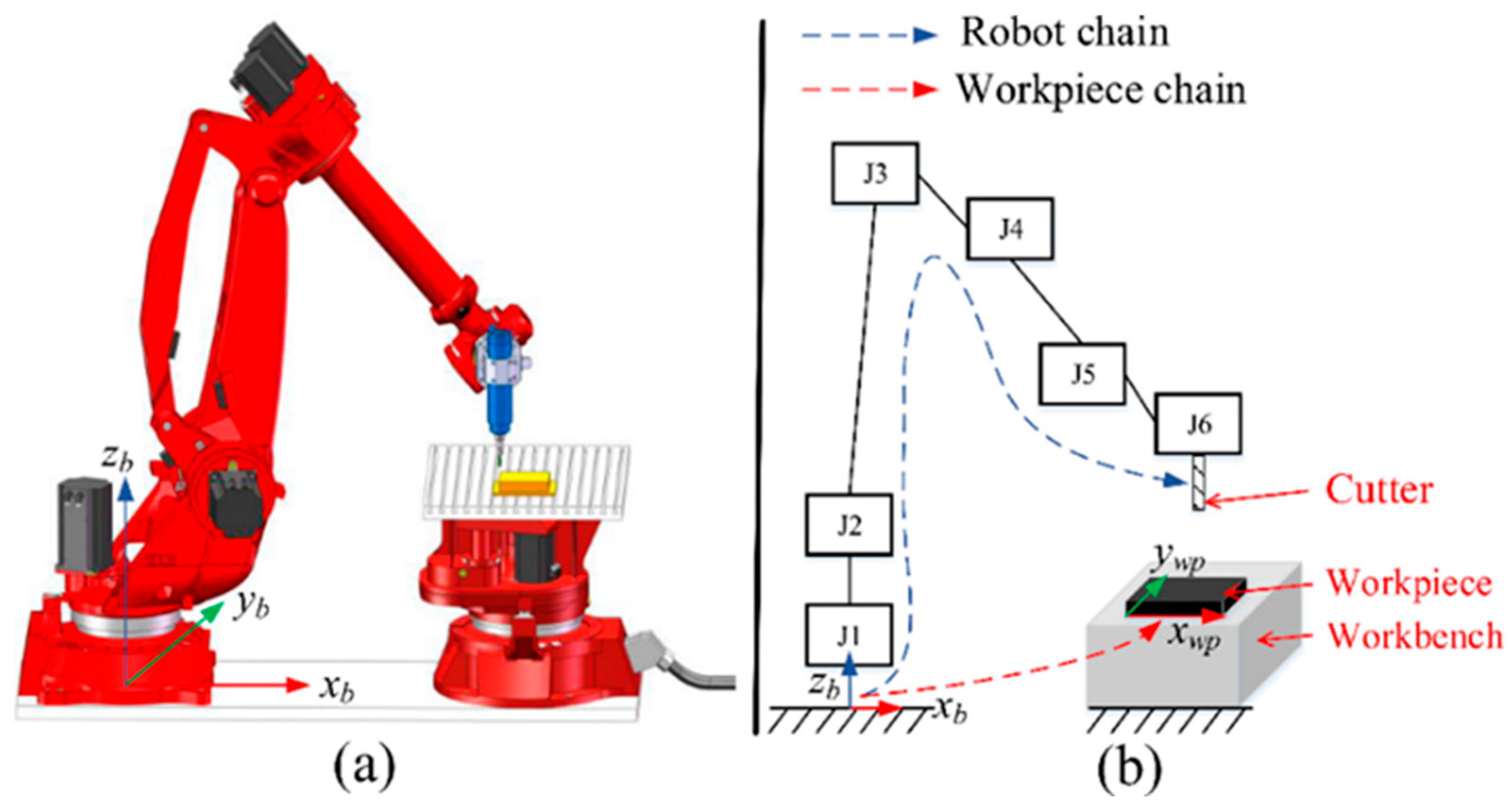
For machining operations, the CL data that are generated from the CAM system are usually expressed in the workpiece frame and require transformation to the robot frame before the process execution [19]. The homogenous transformation of the workpiece frame relative to the robot base frame is
T w p b = T w b b T w p w b
where T w p b is the transformation from the workpiece frame to the robot base frame, T w b b is the transformation between the workbench frame and the robot base frame, and T w p w b is the transformation between the workpiece frame and the workbench frame. An example of the aforementioned frames is depicted in Figure 1. Additionally, in the robot kinematic chain, the transformation matrix of the tool tip frame relative to the robot base frame is calculated as follows:
T t o o l b = T 1 b T 2 1 T 3 2 T 4 3 T 5 4 T 6 5 T t o o l 6
where 1–6 represent the joint numbers, respectively. The Denavit-Hartenberg (DH) approach has been used for the calculation of the transfer matrices between the adjacent coordinate systems, and the transformation matrix T i i 1 can be formulated as:
T i i 1 = cos θ i sin θ i cos a i sin θ i sin a i a i cos θ i sin θ i cos θ i cos a i cos θ i sin a i a i sin θ i 0 sin a i cos a i d i 0 0 0 1
Combining Equations (1) and (2), the transformation of the tool frame relative to the workpiece frame can be expressed as:
T t o o l w p = T w p b 1 T t o o l b
After having defined the workpiece placement position and the CLs along the toolpath, the robot joint values throughout the process can be calculated using the inverse kinematics of the robot as follows:
θ = I K x w p , y w p , a w b
where θ = θ 1 , θ 2 , θ 3 , θ 4 , θ 5 , θ 6 Τ is the motion of the robot joints, x w p , y w p is the positional offset of the workpiece from the workbench, and a w b is the rotational offset of the workbench relative to the robot base frame [14,38].

3.2. Robot Dynamics

The Multi-Body Simulation methods have been adopted extensively for robot dynamic behavior modeling and simulation because of their high accuracy levels and time efficiency when compared to other simulation methods such as finite element. The two main approaches adopted for the modeling of the dynamic behavior of industrial robots are: (a) flexible joints and rigid links and (b) both flexible joints and links. For the model presented in this paper, the second modeling approach has been adopted, combined with the component mode synthesis (CMS) method, to enable accurate simulation of the robot dynamics, while keeping the computation time in acceptable limits for usage during the process planning stage.
In general, the equation describing the robot dynamics for a specific configuration x 0 in the Cartesian space can be expressed as follows:
M x x 0 δ x ¨ t + C x x 0 δ x ˙ t + K x x 0 δ x t = F t
where δ x t ,   δ x ˙ t , δ x ¨ t are the displacement, speed, and acceleration of the end-effector, respectively, with δ x t = x t x 0 the infinitesimal displacement relative to a configuration x 0 ; additionally M ,   C ,   K are the robot mass, damping, and stiffness matrices, respectively, and F t the cutting force vector applied to the cutting tool throughout the process. Moving on to the natural frequencies and mode shapes of the robot arm structure, they can be calculated using the following equation:
K ω 0 i 2 M p i = 0
where ω 0 i are the natural frequencies and p i the mode shapes of the robot [39].

3.2.1. Robot Links Modeling

When link flexibility must be taken into account, FE models have been proven to be an accurate solution, using a significant number of degrees of freedom (DOFs) to calculate the link deflections. However, the number of DOFs used to represent the flexible link must be decreased before their integration with the MBS, to keep the computational cost low. For this purpose, the Craig-Bampton method has been utilized to build the reduced order model of each link [40]. The modeling process followed for the links of the robot is presented extensively below.
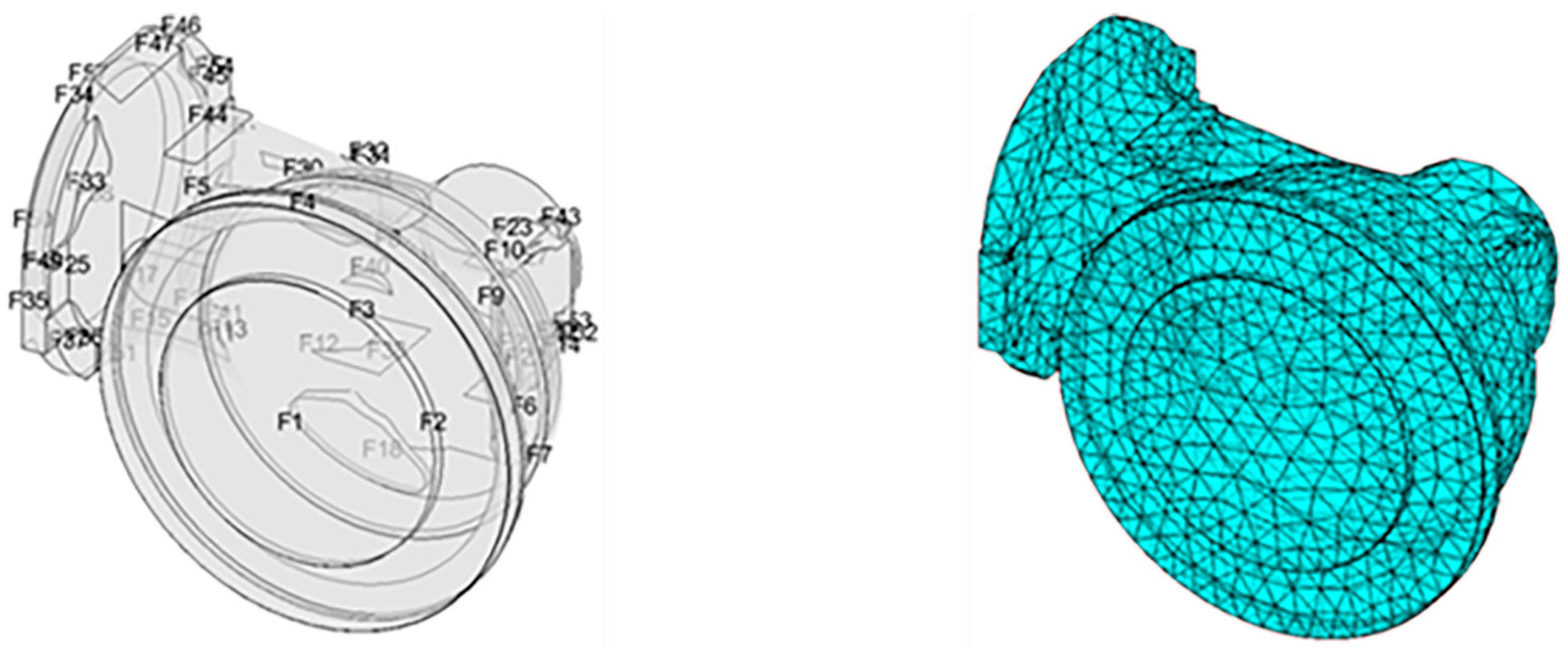
First, the FE models of all links must be created, so their elastic behavior under loading conditions, in addition to their natural frequencies and mode shapes can be considered. Following that, the reduction of the models can be performed using the Craig-Bampton (CB) method. The advantage of this method is that it includes both static and vibration modes to create a complete reduction basis and, subsequently, an appropriate representation of the subsystem’s dynamic behavior. Only vibration modes with natural frequencies in a selected frequency range from the user are retained to approximate the dynamics of the DOFs internal to the substructure, leaving behind only the DOFs at the interfaces, which in this case are connected to the adjacent links through rotational joints, and a certain number of internal DOFs related to the retained vibration modes in a clamped boundary configuration. After the CB method application, the reduced mass and stiffness matrices are obtained, which are known as Superelements in commercial FE packages and are being used to represent the dynamic behavior of flexible bodies [41]. The modeling procedure for the robot links is summarized in Figure 2 below.
Finally, modal damping has been adopted to represent the damping properties of the links, and the damping matrix of every link can be formulated as follows:
C = M Φ 2 ζ ω n Φ Τ M
where M is the mass matrix, 2 ζ ω n is a diagonal matrix, and Φ are the mode shapes of the link substructure.

3.2.2. Robot Joints Modeling

Joint elastic behavior has been identified by many authors as one of the main sources of end-effector positional error during robotic machining operations, affecting directly the process accuracy, and it cannot be neglected. Assuming that joints’ elastic deformation under loading conditions is a function of their stiffness and damping properties [42], the revolute joint of a robot can be modeled as a rotary spring—damper system along its rotation axis. The benefits of this modeling approach is that it can be fully described with only two parameters (spring stiffness and damping coefficient), while no considerable advantages from the use of more complex models with numerous parameters have been identified from the literature [8,43]. Additionally, the influence of servo motors’ inertias has also been taken into account during the modeling phase for the sake of completeness.
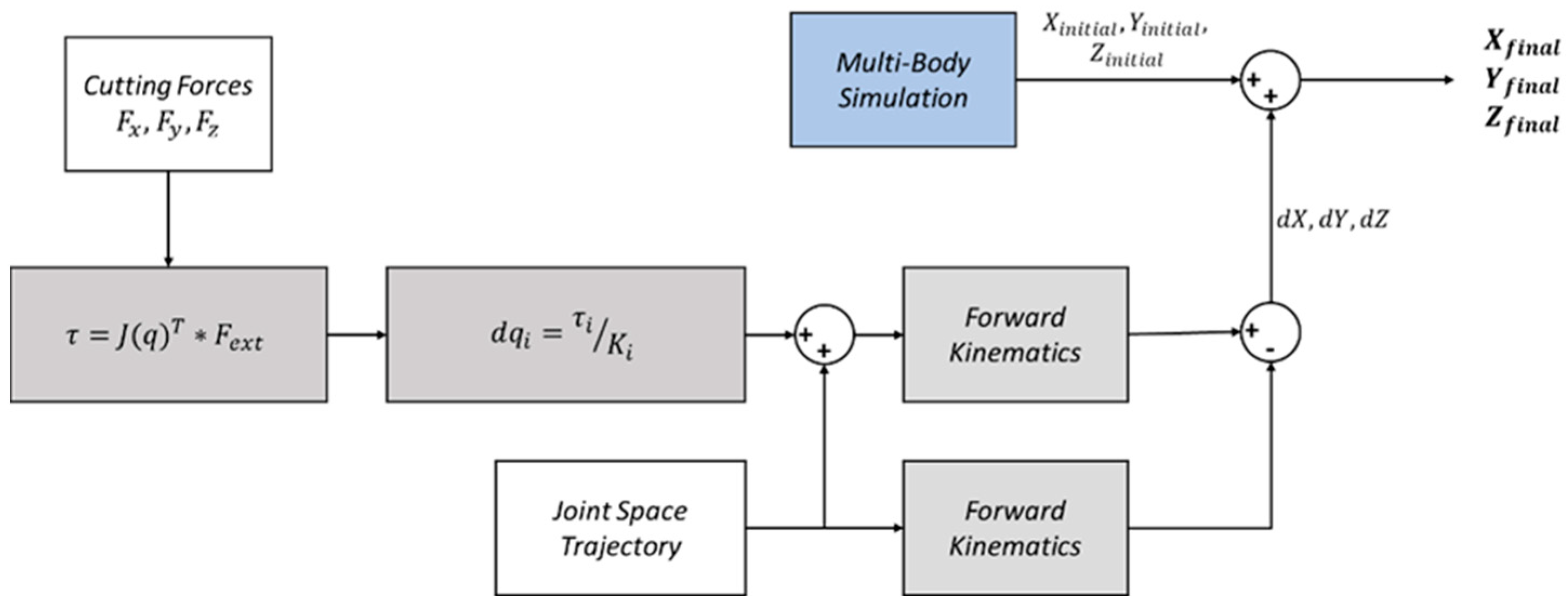
It is important at this point to explain a bit further the approach used to include the joint deformations inside the Multi-Body model. In general, the applied joint motor torques can be calculated as follows:
τ = τ m + τ e x t + τ f
where τ m are the torques demanded to hold position or cause a motion, τ e x t the resultant torques from external forces or torques that must be defeated, and τ f the friction-induced torques. However, since the robot controller does not receive any information regarding the cutting forces applied to the robot during the process and the joint position encoders are placed before the compliant transmission elements, the external forces exerted on the robot end-effector cannot be compensated, leading to joint deformation and, subsequently, to process accuracy loss. The torques applied to joints for a given set of cutting forces can be calculated using the transpose of the robot arm geometric Jacobian as follows [44]:
τ e x t = J q T F e x t
where τ e x t are the torques applied to motors and F e x t are the cutting forces applied to the robot end-effector. Because joints have been approximated with torsional springs, the angular deformation of every joint can be calculated from Hooke’s law as follows:
τ = k d θ   d θ = τ k    
where k is joint spring stiffness value of the joint in N m / r a d , while the minus sign has been omitted because for this model the deformation direction is defined from torque sign. After estimating all six angular deformations, the deformed cutting tool position can be calculated. Figure 3 summarizes the aforementioned procedure with a flowchart.

3.3. Control Logic

Robotic systems combine mechanical, electrical, and software parts to perform the commanded functions; as a result, the controller architecture has a significant impact on the manipulator performance and the applications it can accomplish. A joint space controller has been developed to further extend the robot multi-body model and lead to a more realistic digital representation of the real robot. In addition, a PD controller for every joint has been included to create a closed-loop control system. The architecture of the proposed controller is presented in Figure 4 below.
After taking into account the dynamics of an N non-fixed joints manipulator, the control torque vector can be expressed as follows:
u = M q q ¨ + C q , q ˙ q ˙ + G q ˙
where M q is the joint space mass matrix of the robot, C q , q ˙ q ˙ is the velocity product torque, and G q ˙ is the gravity torque for the specific configuration. Furthermore, due to the PD controllers the above equation can be transformed in the following form:
u = M q q ¨ K d q e ˙ K p q e + C q , q ˙ q ˙ + G q ˙
where q e = q q d is the positional error, q e ˙ = q ˙ q d ˙ is the velocity error, and K p , K d are the diagonal matrices of proportional and derivative gains, respectively [44].
Tuning of the PD controller’s parameters has been based on the requirement to achieve positional error in the order of micrometer, under no loaded motions. For a full description of the behavior of the robotic arm, the actual control algorithm of the robot should have been considered, also incorporating the dynamic response of the mechatronic system of the joints (drives, motors, etc.). However, it was not possible to acquire the knowledge of the actual control system parameters for the specific robot that has been modeled. As such, the minimization of the positional error at no-load motions enables accurately considering only the deflections introduced due to the machining process.

3.4. Implementation

Software implementation of the Digital-Model presented in this section has been performed in the Matlab (R2022b)-Simulink environment, in order to create a fully parametric model, applicable to any six-axis industrial robot. For this work, the developed model has been applied for a robotic cell consisting of a GP225 6-DOF robotic arm from Yaskawa, with a cutting tool and its tool-holder attached to the robot TCP, and a two-axis rotary table for the workpiece placement. The setup of the aforementioned cell is presented in Figure 5 below.
The robot Digital-Model presented in this work is an extension of the model presented in one of the previous works of the authors [45]. Analytical representation of the implementation strategy followed is also included in the aforementioned work. The complete implementation architecture of the DM is presented in Figure 6 below.

3.4.1. Multi-Body Model and Controller

Using the Simulink environment, it has been attempted to create an accurate digital representation of the robot structure by using different blocks for the dynamic behavior representation of its main components. From Section 3.2, it is becoming clear that the joints and the links are the most significant components of the robot to model when its dynamic behavior is examined; as a result, their modeling accuracy is of utmost importance for the MBS. The developed model requires as input the joint angles and the generated cutting forces, and returns the predicted Cartesian position of the cutting tool throughout the process. Those values can be used later for the estimation of the cutting tool positional error during the process, when compared with the toolpath reference positions. The Simulink blocks used for the flexible link representation demand as input the 3D CAD file, the interface node coordinates, and the reduced order mass, stiffness, and damping matrices, or, in other words, the link Superelement. As for the joints’ representative blocks, only the damping coefficient values are required, since the spring stiffness values are imported to the model through the process described in Section 3.2.2.
It is noted that due to a lack of experimental data for this specific Yaskawa robot, the values of Table 1 were obtained from a similar robot of the same manufacturer [12]. According to the literature, general-purpose robots with comparable reach and payload characteristics have similar joint stiffness and damping values [12,46,47]. The following approximations have also been done during the modeling process:
  • The robot base and flange have been modeled as rigid bodies, due to their increased stiffness compared to the robot links.
  • The cutting tool and tool holder have also been modeled as rigid bodies, as well as their interfaces.
  • The joint motors have been modeled as point masses, due to lack of data regarding their actual geometry.
The robot joints torque controller has also been developed in the Simulink environment together with the multi-body model presented above, using the Simulink Robotics System Toolbox. For the estimation of the PD controller parameters, the PID Tuner tool of Simulink has been used, according to the requirement mentioned in Section 3.3.

3.4.2. Auxiliary Software Modules

An integrated Matlab script has also been developed for the flexible links modeling procedure presented in Section 3.2.1. The code receives as input the link geometry, the material characteristics, and the demanded parameters to perform the CB reduction (interface nodes and frequency range) of the robot links FE models (Figure 7). As an outcome, the reduced mass, stiffness, and damping matrices are extracted. After the application of this code for every link of the robot arm, all the necessary Superelements are ready to be imported to the Simulink MBS tool.
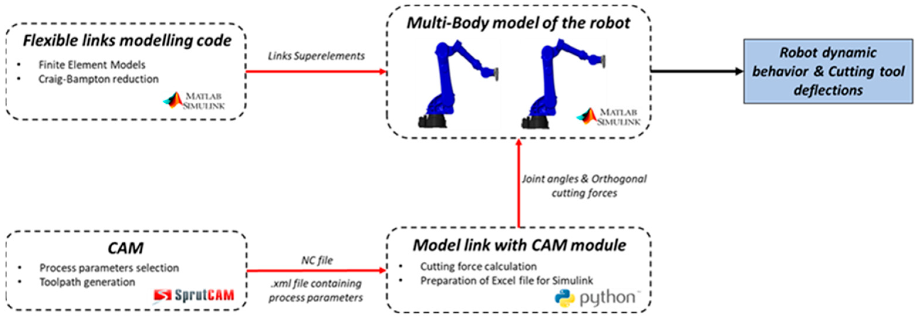
Finally, a Python software module dedicated to the interoperability between the simulation tool and the CAM software (SprutCAM X Robot v16) has been developed. This tool is responsible for the generation of an Excel file that contains the process joint angles and orthogonal cutting forces as a function of time, which serves as an input for the Simulink MBS, after having fully designed the process in the SprutCAM environment (robot and cutting tool geometry, toolpaths, and process parameters). The implementation workflow for the link between the MBS and SprutCAM is presented in Figure 8.
Since SprutCAM does not calculate the generated cutting forces, the Altintas [48] model has been adopted, which provides a fast and flexible modeling approach that takes into account the tool geometry and material, process parameters, workpiece material, and tool orientation. The formulation of the instantaneous cutting forces in the tangential d F t , j , radial ( d F r , j ) , and axial d F a , j direction is presented below:
d F t , j φ j , z = K t e d S z + K t c f z sin φ j d z d F r , j φ j , z = K r e d S z + K r c f z sin φ j d z d F a , j φ j , z = K a e d S z + K a c f z sin φ j d z
From the above equations, it is getting clear that this model considers the cutting forces to be linearly linked with the feed per tooth f z and axial depth of cut z , while being a function of the immersion angle of the j -th cutting edge of the cutting tool φ j . Finally, K   . c are the cutting force coefficients and K   . e the edge force coefficients.

4. Optimization Strategies

4.1. Workpiece Placement Optimization

The position of the machining workpiece relative to the robot has a significant impact on the robot configuration and the generated cutting forces during the process. Therefore, a task-dependent workpiece placement optimization tool is of utmost importance for robotic machining operations. Taking into consideration the posture-dependent dynamic behavior of the robot, and the one redundant DOF even when performing five-axis machining, optimal placement of the workpiece can be seen as an excellent optimization opportunity. A tool able to calculate the optimal position and orientation of the machining part in two stages with respect both to the robot dynamics and the workpiece geometry has been developed, attempting to maximize the robot stiffness along the cutting toolpath.
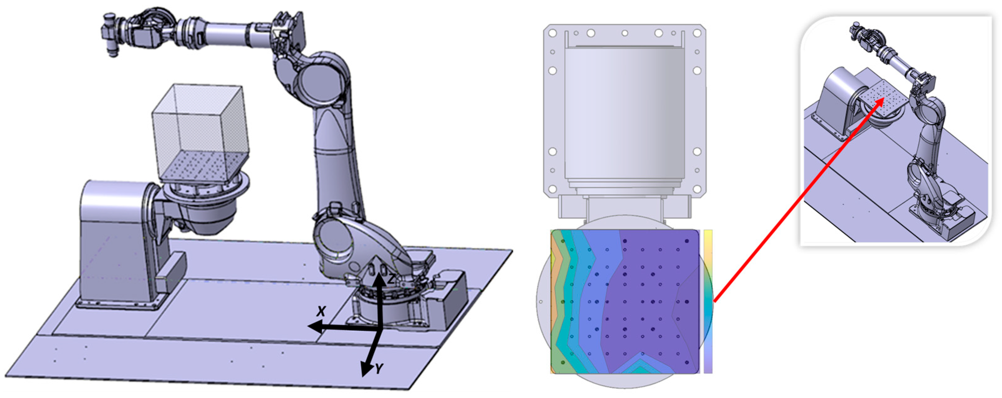
Identifying the stiffness values and how they fluctuate over the working space is essential for maximizing the robot’s stiffness along a trajectory. For this purpose, the stiffness maps of the robot for a cube above the rotary table have been created, using the developed Digital-Model. A series of static simulations in the aforementioned area have been performed in order to calculate the robot stiffnesses along x , y , and z directions. To achieve that, static simulations have been executed using the developed multi-body model to estimate all three axial deflection values in points every 100   mm in the previously mentioned cube and, subsequently, the axial stiffnesses.
The vector of the load applied in Newtons to the robot end-effector in all cases was F = 100 i 100 j + 100 k , with respect to the robot base coordinate frame (Figure 9). The robot stiffness values along x , y , and z directions for every point can now be defined as follows:
X S t i f f n e s s = l o a d x a x i s / d X = 100 / d X     N / m m Y S t i f f n e s s = l o a d y a x i s / d Y = 100 / d Y     N / m m Z S t i f f n e s s = l o a d x a x i s / d Z = 100 / d Z     N / m m
where d X , d Y , and d Z are the robot deflections to the correspondent axis from the initial position during the static simulations. Some of the generated stiffness maps are presented in Figure 10 below, while it is noted that all the coordinate values are measured from the robot base system, and all the simulations have been performed for robot poses that the cutting tool axis is aligned with the robot z axis. It is evident that with the approach followed for the stiffness map generation, the kinematic redundancy of the robot is not taken into account. As such, this tool is not suitable for robot pose optimization applications, but only for selection of the optimal workpiece placement position when machining parts with the aforementioned configuration.
Based on the generated stiffness maps and the part geometrical features, the user can first define and then clamp the workpiece at the stiffer regions before the actual process execution. The goal of this algorithm is to assist the user in the selection of the workpiece placement position and not to define a single optimal position, providing him with the whole background information about the stiffer positions of the robot and giving him the flexibility to consider during the placement selection process and other parameters except robot stiffness (e.g., available working space and ease of stock part clamping).
From the above stiffness maps it is becoming clear that the stiffness values along the robot x-axis are much greater compared to the y-axis. As a result, the orientation of the workpiece can be tuned, so that the highest machining loads are aligned with the x-axis of the robot. Due to the increased stiffness in the x-axis, less machining error and increased part quality is expected. Based on that, an integrated MATLAB script has been developed to estimate the workpiece optimal orientation, using the toolpath points of a finishing process, and attempting to align in an efficient way the robot x axis with the contour error vector. Specifically, the normal vectors along the given toolpath, the angles between those vectors and robot x axis, and the mean value of the angles are calculated. Then, the rotation of the machined part starting from the x axis and moving counterclockwise is calculated from the following equation in degrees:
R o t a t i o n _ A n g l e = 180 M e a n _ V a l u e
In the next section, an optimization strategy for one for most influential process parameters is presented, in an attempt to further increase the accuracy of robotic machining applications.

4.2. Feed-Rate Scheduling

As already discussed, industrial robots are seldom used by industry for machining applications, mainly due to their compromised stiffness when compared with conventional CNC machines. Feed-rate scheduling algorithms applied in robotic machining operations attempt to calculate a proper upper limit for the feed rate, to eliminate excessive contour error values outside the demanded part tolerance, due to deformation and vibration of the robot structure, while maintaining a high enough material removal rate [17].
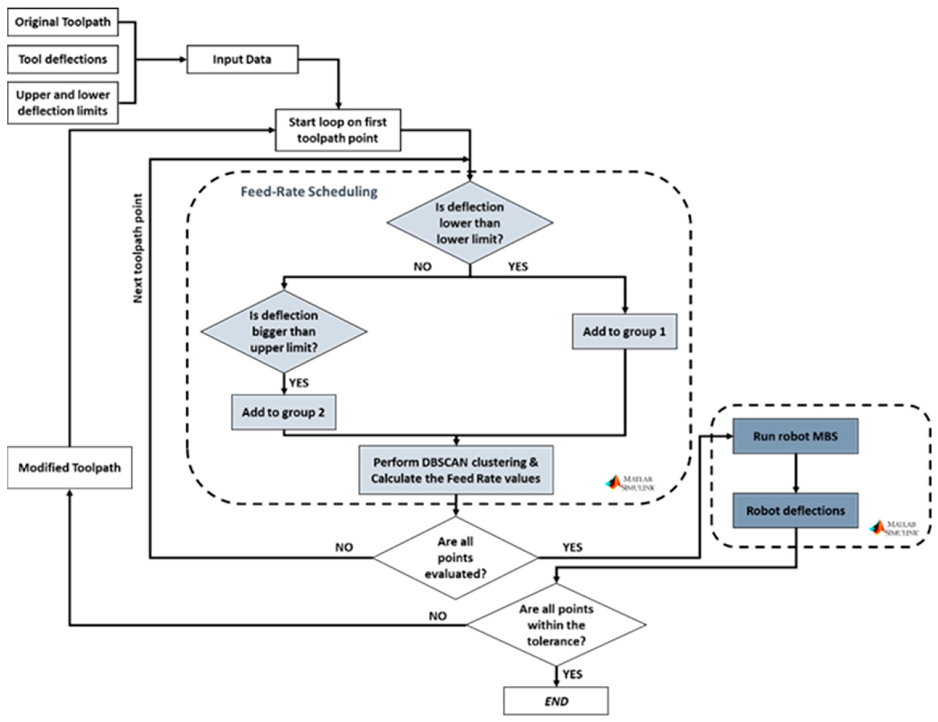
An offline feed-rate scheduling method based on a set of precalculated cutting tool deviations along a milling toolpath has been developed using Matlab environment. The algorithm calculates an optimized feed-rate profile for the process, in order to fulfill the user-predefined tolerance requirements, while not sacrificing process productivity. This work is backed up by the Altintas model [48], according to which by lowering the feed rate and lower generated cutting forces can be achieved, due to their linear relationship, which is visible from Equation (14). Lower cutting forces lead to smaller cutting tool positional errors, due to robot limited stiffness. The developed algorithm first performs a two-stage clustering procedure to the toolpath points based on their calculated position deflections and their Cartesian position, to generate regions along the toolpath with similar deflection values, whose feed-rate values must subsequently be modified in a similar way. For points with positional error greater than a user-defined upper limit, the feed rate will be decreased, while for points with error values below a desired lower limit, the feed rate will be increased, in order to enable higher productivity when the accuracy of the part is not that critical. The flowchart of the feed-rate scheduling algorithm is presented in detail in Figure 11 below.
A linear relationship between the cutting forces and the feed rate has been assumed for the calculation of the adjusted feed-rate values, since this approach has been proved to return reasonable results for the new feed-rate values, without introducing any additional complexities [49]. The calculation formula used for the calculation of the new feed rate is:
F R n e w = F R o l d × F max _ d e s i r e d F max _ a p p l i e d
where F max _ a p p l i e d is the maximum force applied along the y-axis between the points of every cluster and F max _ d e s i r e d is a user-selected value based on the demanded tolerance and robot stiffness maps for the y axis and F R o l d the initial selected feed-rate value. It is evident that this algorithm aims to reduce the cutting forces at points with big loads along the robot y axis, due to the compromised robot stiffness at this direction. The above equation is being used only for the points whose feed rate needs to be decreased, while the feed rate of all points with deflections lower than the lower limit is increasing by 50 % from the initial value that the user has selected for the feed rate.
It is noted that the algorithm has been proven to efficiently reduce the number of points with unacceptable deflection values; however, it is not able to eliminate them. This lies in the fact that the contribution of the feed rate to the generated cutting forces values is limited, while other parameters (axial depth of cut, radial engagement) are also important to the overall cutting force value. Significantly wrong selection of these parameters cannot be compensated by only tweaking the feed rate.

5. Case Studies for Model and Optimizations Testing

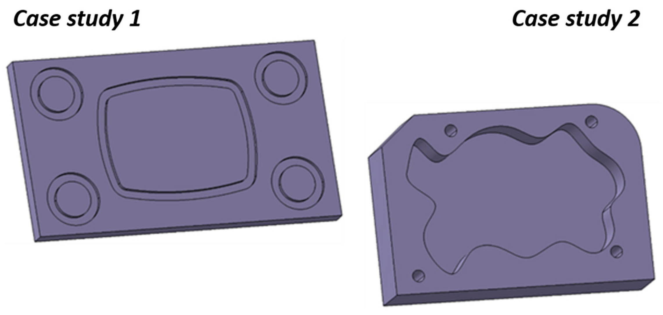
Two different case-studies are presented in this section to demonstrate the abilities of the developed model and optimization algorithms. The 3D CAD models of the case-study parts are shown in Figure 12. Case Study 1 aims to highlight the robot posture-dependent dynamic behavior using the developed model, while Case Study 2 attempts to present the effect of the optimization algorithms to the process accuracy.
The process parameters used for the process design in the SprutCAM environment are presented in Table 2 below, while it is noted that a cutting tool with a 10   mm diameter has been used in all cases.

5.1. Case Study 1

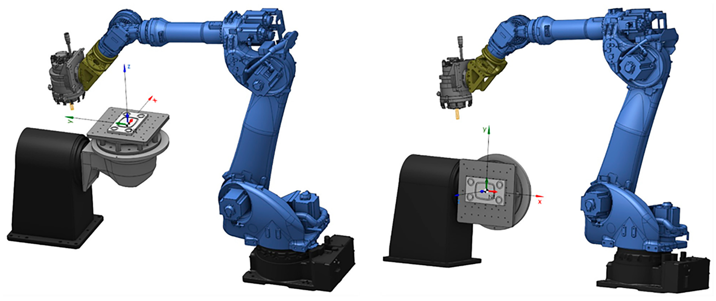
Two different simulations have been executed in this case study for the same part with two different workpiece placement setups, to investigate the effect of the robot posture and workpiece placement position to the final process accuracy.
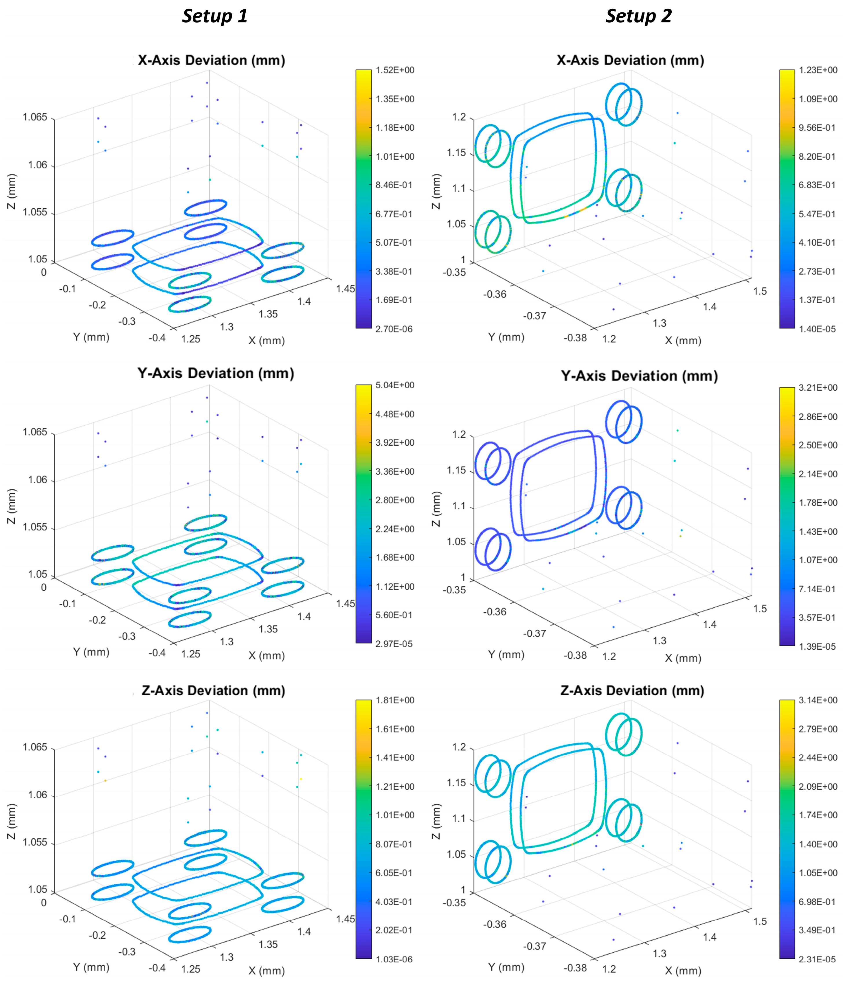
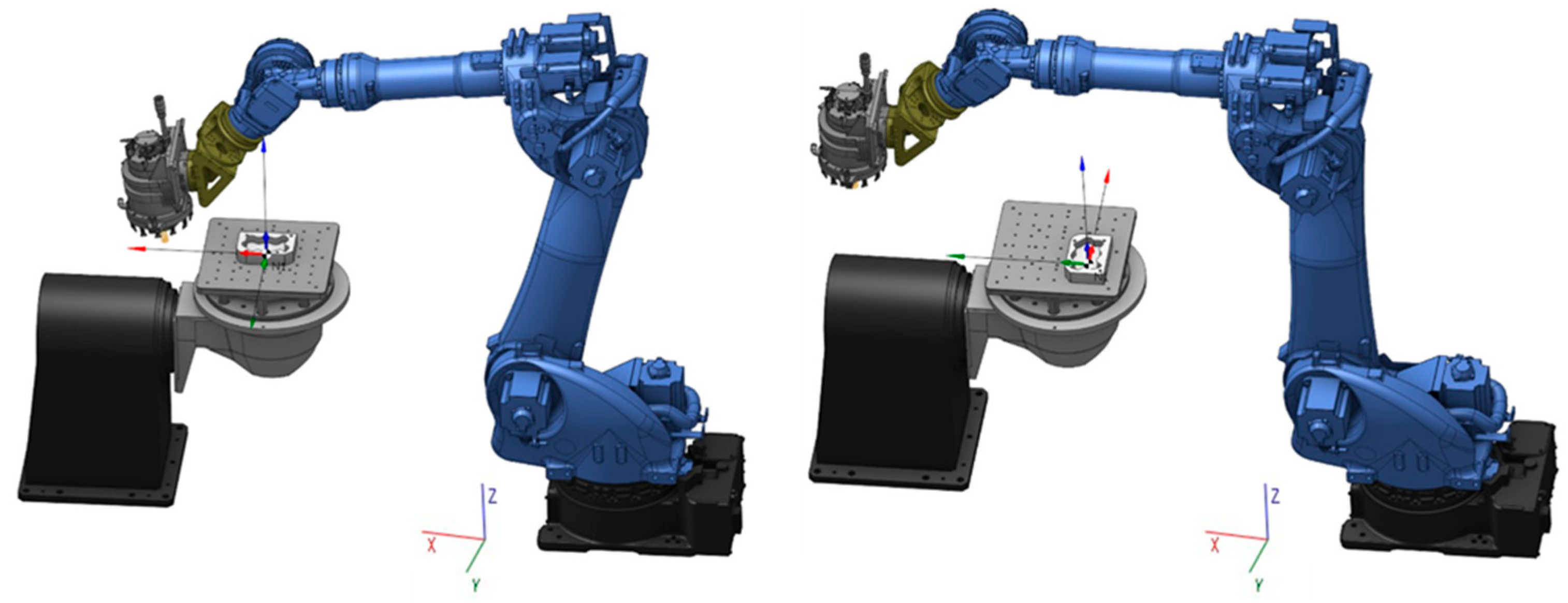
The calculated maximum and mean positional deviations of the cutting tool in all three directions ( x ,   y ,   z ) are displayed in Table 3. It is noted that for this case the x , y and z directions are referring to the local rotating coordinate system of the part ( x y z as shown in Figure 13).
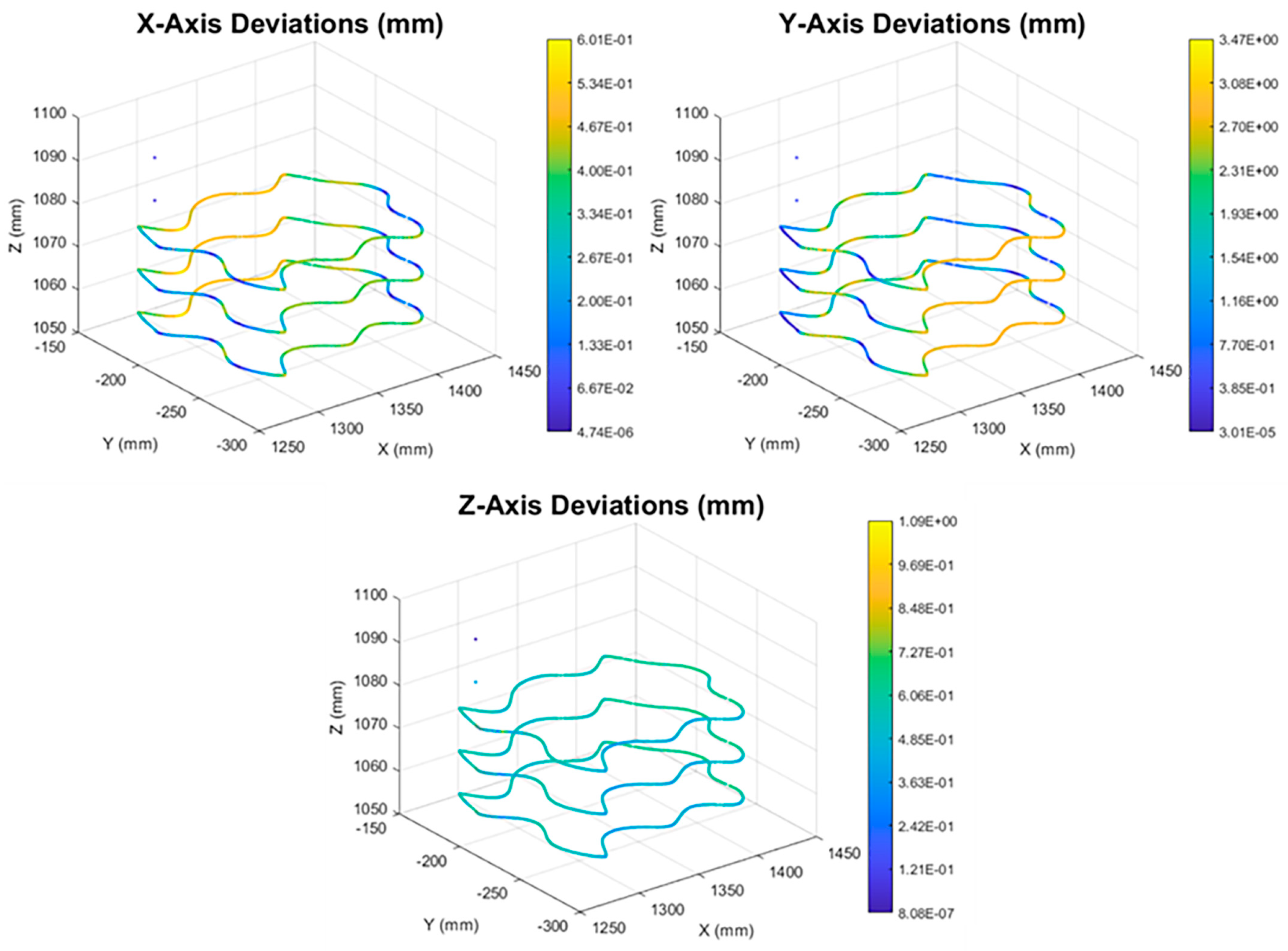
From the results above, it is evident that the deviations are comparable for both setups; however, the variations between the cases range from 0.06   mm up to almost 2   mm . Since the only difference between the two simulated setups is the workpiece clamping position, it is concluded that those variations are introduced only from the robot posture-dependent dynamic behavior. The deviation values along the cutting toolpath are also presented in the colormaps below (Figure 14) to enable better understanding and comparison of the simulation results. It is noted that the toolpaths that are presented in the figure below are also the toolpaths used for the machining of the correspondent part. These toolpaths correspond to the finishing operations of the pockets, since these are the ones of interest to be modeled.

5.2. Case Study 2

Simulation of the machining process demanded to generate the part of Case Study 2 has been executed twice. First, by placing the workpiece in the center of the rotary table and with an arbitrary orientation, and, subsequently, after the application of both optimization algorithms discussed in Section 4, in an effort to calculate the process accuracy improvements introduced from their application during the process planning stage.
Initially, the workpiece placement optimization has been applied, attempting to increase the process accuracy by placing the workpiece at the region with the greater robot stiffness, while the workpiece optimal orientation algorithm has estimated that the part must be rotated by 89.9   degrees clockwise. Following that, the feed-rate scheduling algorithm has been applied for further improvement of the process accuracy. For this case, the tolerance value has been selected to be 1.5   mm and the lower limit to be 0.75   mm . With the application of the algorithm, the toolpath points with deviations above the tolerance value have been decreased from 1287 to 597 , while the process time has been increased from 48 to 60   s . The results from the simulations before and after the application of the optimization algorithms are summarized in Table 4 below, with x , y and z directions referring to the global coordinate system of the robot ( x y z as shown in Figure 15).
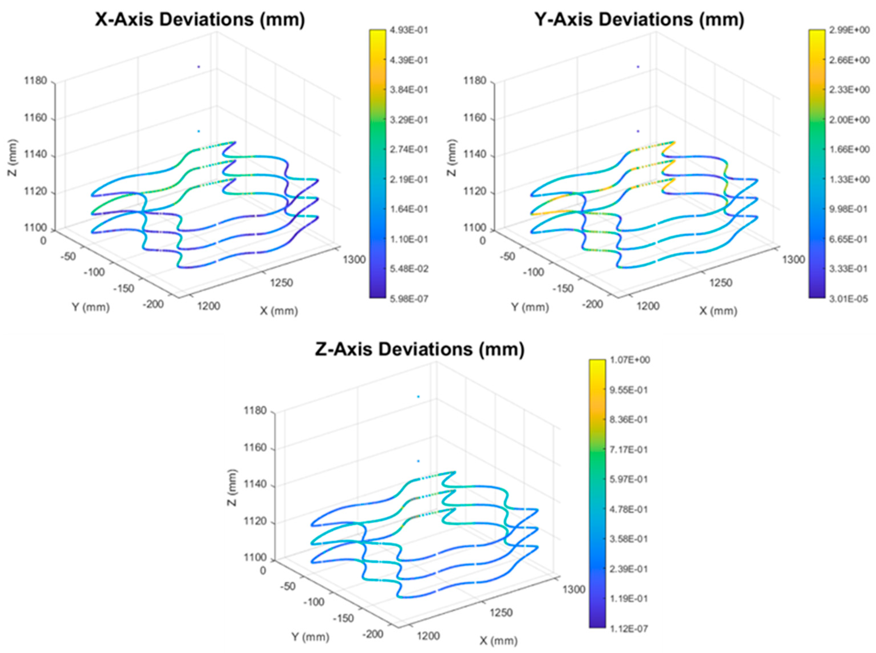
It is noted that any of the two optimization algorithms proposed in this work can also be implemented on its own; however, from the simulation experiments conducted it is concluded that the best process accuracy is obtained when both optimization algorithms are applied. The deviation colormaps for the two scenarios are presented below in Figure 16 and Figure 17. It is noted that the toolpaths that are presented in the two figures below are the finishing toolpaths required for the machining of the parts, which are also the simulated toolpaths.
From Case Study 2, the two following conclusions can be extracted regarding the effect of the optimization algorithms to the process accuracy obtained from the process simulation:
  • Deviations along the robot y axis are the main source of positional error, both before and after the application of the optimization algorithms.
  • Deviations along the robot x axis are improved the most from the application of the process optimization algorithms.

6. Experimental Validation

After having completed the development of the machining robot DM, it is essential to verify that the model’s outputs closely match actual experimental data and the optimization algorithms can improve the parts’ accuracy in real machining scenarios. Experimental validation of the model is necessary to ensure its accuracy and reliability by comparing the model outputs with real-world data and should be performed before the adoption of the model by any potential industrial users. To achieve this, a significant number of side milling experiments were conducted for various sets of process parameters, with different cutting directions and robot configurations, to collect a comprehensive dataset for the dynamic behavior of the robot during milling operations. The side milling experiments were always machining passes in a straight line. Each experiment number corresponds to a single machining pass performed with the process parameters described in Table 5. The selection of different cutting parameters (and thus different induced cutting forces) examines the linearity of the physical system, in response to the load variation. The DM, implemented in Simulink, is inherently linear due to the use of the linear spring damper systems for the joints and the method of generating the stiffness and damping matrices of the members. Additionally, the inclusion of experiments with various cutting directions and robot configurations aims to verify the model’s ability to successfully predict the pose-dependent stiffness of the robot arm throughout the working space.
The material used in all experiments was Aluminum 7075-T651, while the cutting tool was a R390-016A16-11L indexable end mill from Sandvik Coromant (Sandviken, Sweden) with R390-11 T3 04E-NL H13A inserts from the same manufacturer. In order to evaluate the dependence of the robot dynamic behavior with the robot configuration, experiments were carried with four different configurations:
  • Robot Configuration 1: Movement of the robot along the robot y axis (angle R Z = 0 )
  • Robot Configuration 2: Movement of the robot along the robot x axis (angle R Z = 0 )
  • Robot Configuration 3: Movement the robot along the y axis (angle R Z = 30 ° )
  • Robot Configuration 4: Move the robot along the robot x axis with the table rotated −30° (angle R Z = 60 ° )
The aforementioned robot configurations are presented in Figure 18, while the cutting parameters for each of the 23 total milling experiments can be found in Table 5. All process parameters values (feed per tooth, cutting speed, axial and radial depths of cut) were selected based on the working parameters window provided by the cutting tool manufacturer. There was no specific design of experiments methodology (e.g., factorial, Taguchi) selected for the identification of process parameter combinations, as the point of these experimental tests was just to compare the results against the simulation and not do any further statistical analysis afterwards.
It is noted that in addition to the process parameters mentioned in the table above, for all the experiments the feed per tooth was 0.09   mm and the spindle speed 11,000   RPM .
At the end of every experiment, the dimensions of the machined workpiece were measured to the perpendicular direction of the feed (M1) and to the axial direction of the cutting tool (M2). Those measurements were used later for comparison with the positional error predicted by the DM. The results of the comparison are presented in Table 6 below.
It is evident that, with certain exceptions, the error predictions of the DM have small deviations from the measured values. It is noted that during experiments 22 and 23 the effect of chatter was present during the machining process; therefore, the robot was in a resonant state. The linear approach of the Multi-Body simulation adopted for the development of this DM is not able to simulate this situation with sufficient accuracy. The non-linearity of the robot vibrations when chatter takes place is something that is not yet accounted for in the proposed approach.
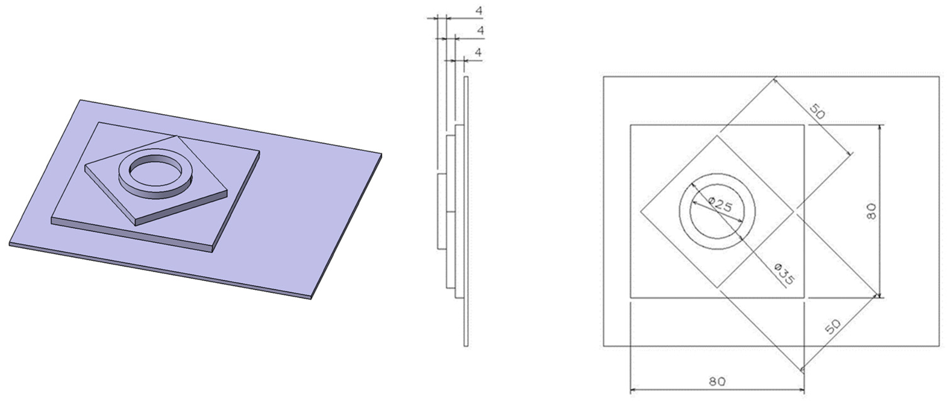
In order to further extend the validation of the developed model, the machining of a standardized part has been simulated and the optimization algorithms have been applied afterwards to validate their added value to real machining scenarios. The part that has been selected follows the NAS979 standard [50] and is widely known as Circle-Diamond-Square (Figure 19), due to its distinctive geometry. The aforementioned part has been selected since it is a standardized specimen for evaluating the accuracy of CNC machine tools.
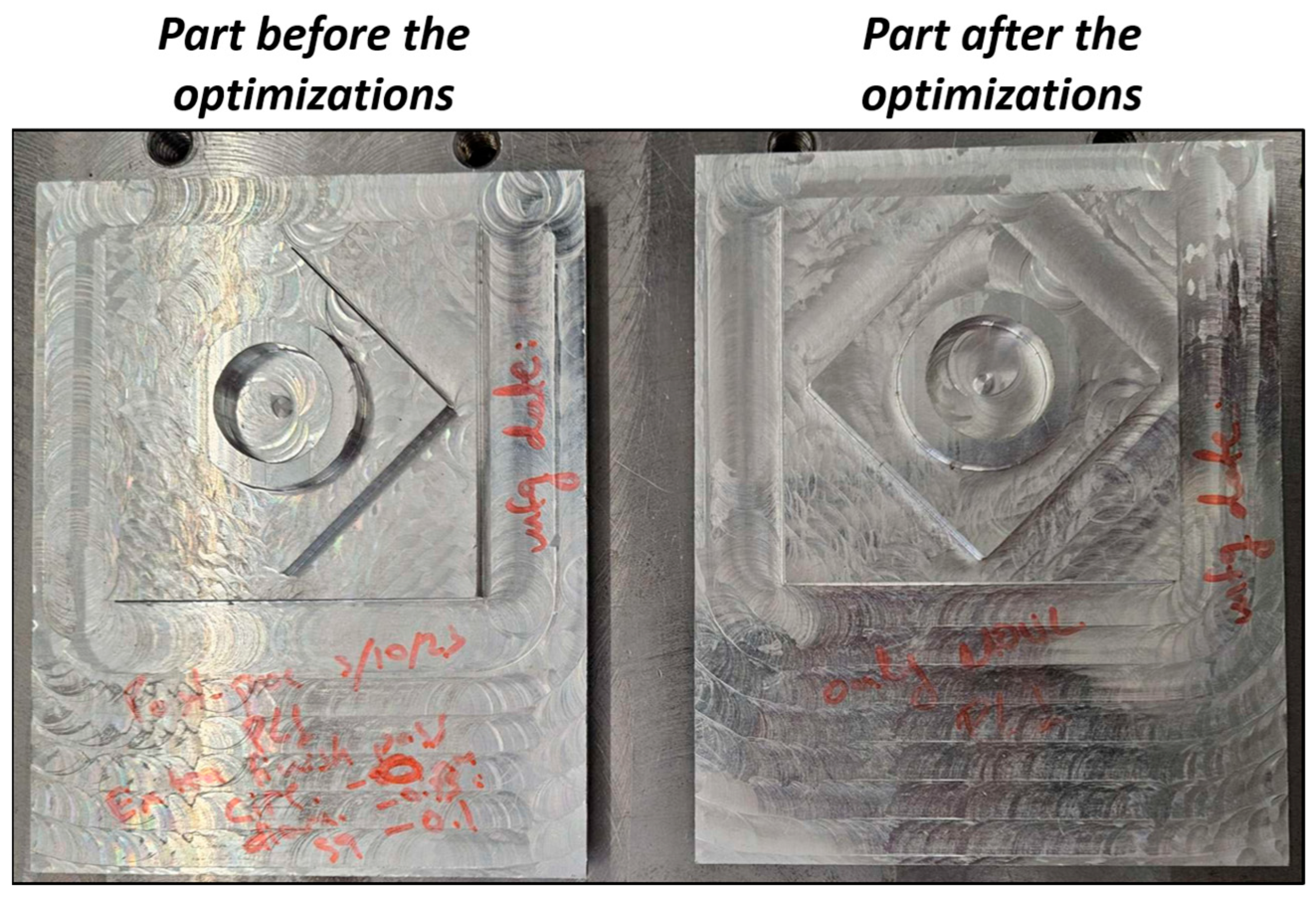
A first test part has been machined using an arbitrary placement position, and its dimensions have been measured. Afterwards, the optimization algorithms were applied and a part has been manufactured again, to prove the part accuracy improvement after their application. Figure 20 presents the setup of the machining experiments before and after the application of the optimization algorithms.
After the machining of the Circle-Diamond-Square parts with both the initial and the optimized setup, their dimensions per feature were measured (Figure 21) for comparison with the DM calculated accuracy results. It is noted that both parts have been manufactured with the same process parameters, except the feed rate which for the part after the optimizations was variable, according to the correspondent algorithm output.
For the results comparison, the mean values of the DM calculated robot deviations in the machining plane per feature (circle, diamond, square) have been used. The simulation results are summarized in Table 7 below.
It is evident that after the application of the optimization algorithms, the manufactured part accuracy has been improved both in the simulations as well as in the actual machining experiments. The two manufactured Circle-Diamond-Square parts are presented in Figure 22 below.
7. Conclusions

This work presents the development of a complete module for robotic machining, which can be coupled with the process planning stage and evaluate the process results and increase its accuracy, decreasing the demand of costly and time-consuming experiments. The DM for a machining robot that is able to simulate its posture-dependent dynamic behavior during the process has been developed, along with two process optimization algorithms. Based on the investigations that have been performed within this work and the results obtained, the following conclusions can be drawn:
  • Link of the DM with the CAM system is mandatory to enable easy implementation of changes during the process planning stage, providing a tool for virtual assessment and optimization of the process.
  • The robot arm has been proven to be much more compliant along its y-axis compared to x-axis, and this must be considered during the process planning.
  • The simulation results validate the increase of the process accuracy after the application of the two optimization algorithms during the process planning stage.
  • From the experimental model validation, it is concluded that the DM can effectively predict the robot positional error for stable machining operations.
  • From the experimental validation of the optimization algorithms, it is concluded that the parts accuracy can be improved, both in simulations and in real machining experiments.
  • The proposed DM is not suitable for the simulation of milling operations where chatter effect is present, due to excess calculation errors. This is sourced from the linear approach adopted for the Multi-Body simulation.
  • Explicit coupling of the machining forces estimation module and the dynamics simulation of the robot has been assumed, meaning that fluctuation in the forces with variation to chip thickness is ignored. However, from experimental validation results it is evident that the experimental and estimated deviations are close; as such, this assumption does not reduce significantly the model’s accuracy. Implicit coupling will be required in order to perform surface morphology analysis.
The most important step that should be taken toward future work is the expansion of the experimental validation of the DM with more and more complex milling geometries and the experimental calculation of the robot joint stiffness and damping values for the used robot. Finally, connection protocols that enable automatic exchange of information between the real robot and the Digital-Model should be developed to construct the complete Digital-Twin of the machining system.

Author Contributions

C.G.: Formal analysis, Methodology, Investigation, Data Curation, Software, Visualization, Writing—original draft, T.S.: Formal analysis, Methodology, Investigation, Data Curation, Writing—original draft, H.B.: Formal analysis, Validation, Visualization, Writing—original draft, P.S.: Conceptualization, Funding acquisition, Validation, Project administration, Resources, Writing—review and editing. All authors have read and agreed to the published version of the manuscript.

Funding

This research received no external funding.

Data Availability Statement

The datasets presented in this article are not readily available because of confidentiality issues. Requests to access the datasets should be directed to the corresponding author.

Acknowledgments

This work has been partially supported by the European Regional Development Fund of the European Union and Greek national funds through the Operational Program Competitiveness, Entrepreneurship and Innovation, under the call RESEARCH—CREATE—INNOVATE (project code: Τ2EDK-03896).

Conflicts of Interest

On behalf of all authors, the corresponding author states that there are no conflicts of interest.

References

  1. Liu, J.; Zhou, H.; Liu, X.; Tian, G.; Wu, M.; Cao, L.; Wang, W. Dynamic Evaluation Method of Machining Process Planning Based on Digital Twin. IEEE Access 2019, 7, 19312–19323. [Google Scholar] [CrossRef]
  2. Stavropoulos, P.; Mourtzis, D. Digital twins in industry 4.0. In Design and Operation of Production Networks for Mass Personalization in the Era of Cloud Technology; Elsevier: Amsterdam, The Netherlands, 2022; pp. 277–316. [Google Scholar] [CrossRef]
  3. Verl, A.; Valente, A.; Melkote, S.; Brecher, C.; Ozturk, E.; Tunc, L.T. Robots in machining. CIRP Ann. 2019, 68, 799–822. [Google Scholar] [CrossRef]
  4. Wang, W.; Guo, Q.; Yang, Z.; Jiang, Y.; Xu, J. A state-of-the-art review on robotic milling of complex parts with high efficiency and precision. Robot. Comput. Manuf. 2023, 79, 102436. [Google Scholar] [CrossRef]
  5. Stavropoulos, P.; Bikas, H.; Avram, O.; Valente, A.; Chryssolouris, G. Hybrid subtractive–additive manufacturing processes for high value-added metal components. Int. J. Adv. Manuf. Technol. 2020, 111, 645–655. [Google Scholar] [CrossRef]
  6. Stavropoulos, P.; Manitaras, D.; Bikas, H.; Souflas, T. Integration of Machining Process Digital Twin in Early Design Stages of a Portable Robotic Machining Cell. In Flexible Automation and Intelligent Manufacturing: The Human-Data-Technology Nexus; Kim, K.-Y., Monplaisir, L., Rickli, J., Eds.; Lecture Notes in Mechanical Engineering; Springer International Publishing: Cham, Switzerland, 2023; pp. 301–315. [Google Scholar] [CrossRef]
  7. Pandremenos, J.; Doukas, C.; Stavropoulos, P.; Chryssolouris, G. Machining with Robots: A Critical Review. In Proceedings of the DET2011 7th International Conference on Digital Enterprise Technology, Athens, Greece, 28–30 September 2011; pp. 1–9. [Google Scholar]
  8. Huynh, H.N.; Assadi, H.; Rivière-Lorphèvre, E.; Verlinden, O.; Ahmadi, K. Modelling the dynamics of industrial robots for milling operations. Robot. Comput. Manuf. 2020, 61, 101852. [Google Scholar] [CrossRef]
  9. Chen, C.; Peng, F.; Yan, R.; Fan, Z.; Li, Y.; Wei, D. Posture-dependent stability prediction of a milling industrial robot based on inverse distance weighted method. Procedia Manuf. 2018, 17, 993–1000. [Google Scholar] [CrossRef]
  10. Brüning, J.; Denkena, B.; Dittrich, M.; Park, H.-S. Simulation Based Planning of Machining Processes with Industrial Robots. Procedia Manuf. 2016, 6, 17–24. [Google Scholar] [CrossRef]
  11. Ma, S.; Deng, K.; Lu, Y.; Xu, X. Robot error compensation based on incremental extreme learning machines and an improved sparrow search algorithm. Int. J. Adv. Manuf. Technol. 2023, 125, 5431–5443. [Google Scholar] [CrossRef]
  12. Chen, Q.; Zhang, C.; Hu, T.; Zhou, Y.; Ni, H.; Xue, X. Posture optimization in robotic machining based on comprehensive deformation index considering spindle weight and cutting force. Robot. Comput. Manuf. 2021, 74, 102290. [Google Scholar] [CrossRef]
  13. Xu, L.; Mao, W.; Zhu, L.; Xu, J.; Sun, Y. Tool orientation and redundancy integrated planning method constrained by stiffness for robotic machining of freeform surfaces. Int. J. Adv. Manuf. Technol. 2022, 121, 8313–8327. [Google Scholar] [CrossRef]
  14. Ye, C.; Yang, J.; Zhao, H.; Ding, H. Task-dependent workpiece placement optimization for minimizing contour errors induced by the low posture-dependent stiffness of robotic milling. Int. J. Mech. Sci. 2021, 205, 106601. [Google Scholar] [CrossRef]
  15. Zerun, Z.; Chen, C.; Fangyu, P.; Xianyin, D.; Dequan, W. Identification of joint position-dependent stiffness parameters and analysis of robot milling deformation. Int. J. Adv. Manuf. Technol. 2022, 118, 4179–4193. [Google Scholar] [CrossRef]
  16. Gotlih, J.; Brezocnik, M.; Karner, T. Stiffness-Based Cell Setup Optimization for Robotic Deburring with a Rotary Table. Appl. Sci. 2021, 11, 8213. [Google Scholar] [CrossRef]
  17. Sun, Y.; Jia, J.; Xu, J.; Chen, M.; Niu, J. Path, feedrate and trajectory planning for free-from surface machining: A state-of-the-art review. Chin. J. Aeronaut. 2021, 35, 12–29. [Google Scholar] [CrossRef]
  18. Xiong, G.; Li, Z.-L.; Ding, Y.; Zhu, L. Integration of optimized feedrate into an online adaptive force controller for robot milling. Int. J. Adv. Manuf. Technol. 2020, 106, 1533–1542. [Google Scholar] [CrossRef]
  19. Cordes, M.; Hintze, W.; Altintas, Y. Chatter stability in robotic milling. Robot. Comput. Manuf. 2019, 55, 11–18. [Google Scholar] [CrossRef]
  20. Li, J.; Li, B.; Shen, N.; Qian, H.; Guo, Z. Effect of the cutter path and the workpiece clamping position on the stability of the robotic milling system. Int. J. Adv. Manuf. Technol. 2017, 89, 2919–2933. [Google Scholar] [CrossRef]
  21. Wu, J.; Peng, F.; Tang, X.; Yan, R.; Xin, S.; Mao, X. Characterization of milling robot mode shape and analysis of the weak parts causing end vibration. Measurement 2022, 203, 111934. [Google Scholar] [CrossRef]
  22. Mohammadi, Y.; Ahmadi, K. Chatter in milling with robots with structural nonlinearity. Mech. Syst. Signal Process. 2022, 167, 108523. [Google Scholar] [CrossRef]
  23. Swan, R.; Penney, J.; Corson, G.; Nazario, J.; Schmitz, T. Surface location error in robotic milling: Effect of combined low frequency and high frequency vibration modes. CIRP J. Manuf. Sci. Technol. 2024, 49, 203–215. [Google Scholar] [CrossRef]
  24. Tunc, L.T.; Gonul, B. Effect of quasi-static motion on the dynamics and stability of robotic milling. CIRP Ann. 2021, 70, 305–308. [Google Scholar] [CrossRef]
  25. Busch, M.; Schnoes, F.; Elsharkawy, A.; Zaeh, M.F. Methodology for model-based uncertainty quantification of the vibrational properties of machining robots. Robot. Comput. Manuf. 2022, 73, 102243. [Google Scholar] [CrossRef]
  26. Huynh, H.N.; Assadi, H.; Dambly, V.; Rivière-Lorphèvre, E.; Verlinden, O. Direct method for updating flexible multibody systems applied to a milling robot. Robot. Comput. Manuf. 2021, 68, 102049. [Google Scholar] [CrossRef]
  27. Chen, H.; Ahmadi, K. Estimating pose-dependent FRF in machining robots using multibody dynamics and Gaussian Process Regression. Robot. Comput. Manuf. 2022, 77, 102354. [Google Scholar] [CrossRef]
  28. Wang, R.; Li, F.; Niu, J.; Sun, Y. Prediction of pose-dependent modal properties and stability limits in robotic ball-end milling. Robot. Comput. Manuf. 2022, 75, 102307. [Google Scholar] [CrossRef]
  29. Karim, A.; Hitzer, J.; Lechler, A.; Verl, A. Analysis of the dynamic behavior of a six-axis industrial robot within the entire workspace in respect of machining tasks. In Proceedings of the 2017 IEEE International Conference on Advanced Intelligent Mechatronics (AIM), Munich, Germany, 3–7 July 2017; pp. 670–675. [Google Scholar] [CrossRef]
  30. Mejri, S.; Gagnol, V.; Le, T.-P.; Sabourin, L.; Ray, P.; Paultre, P. Dynamic characterization of machining robot and stability analysis. Int. J. Adv. Manuf. Technol. 2016, 82, 351–359. [Google Scholar] [CrossRef]
  31. Xu, P.; Yao, X.; Liu, S.; Wang, H.; Liu, K.; Kumar, A.S.; Lu, W.F.; Bi, G. Stiffness modeling of an industrial robot with a gravity compensator considering link weights. Mech. Mach. Theory 2021, 161, 104331. [Google Scholar] [CrossRef]
  32. Chen, K.; Xu, P.; Li, B. Interactive coupling of structural dynamics and milling forces for high-frequency stability prediction in robotic milling. Robot. Comput. Manuf. 2024, 86, 102676. [Google Scholar] [CrossRef]
  33. Liao, Z.-Y.; Wu, J.-Z.; Wu, H.-M.; Xie, H.-L.; Wang, Q.-H.; Zhou, X.-F. Profile Error Estimation and Hierarchical Compensation Method for Robotic Surface Machining. IEEE Robot. Autom. Lett. 2024, 9, 3195–3202. [Google Scholar] [CrossRef]
  34. Tepper, C.; Matei, A.; Zarges, J.; Ulbrich, S.; Weigold, M. Optimal design for compliance modeling of industrial robots with bayesian inference of stiffnesses. Prod. Eng. 2023, 17, 643–651. [Google Scholar] [CrossRef]
  35. Celikag, H.; Sims, N.D.; Ozturk, E. Cartesian Stiffness Optimization for Serial Arm Robots. Procedia CIRP 2018, 77, 566–569. [Google Scholar] [CrossRef]
  36. Doukas, C.; Pandremenos, J.; Stavropoulos, P.; Foteinopoulos, P.; Chryssolouris, G. On an Empirical Investigation of the Structural Behavior of Robots. Procedia CIRP 2012, 3, 501–506. [Google Scholar] [CrossRef]
  37. Kratena, T.; Vavruska, P.; Sveda, J.; Valasek, M. Postprocessor for Verification of Robot Movements with Additional Axis after Toolpath Optimization. Procedia CIRP 2021, 101, 154–157. [Google Scholar] [CrossRef]
  38. Lin, J.; Ye, C.; Yang, J.; Zhao, H.; Ding, H.; Luo, M. Contour error-based optimization of the end-effector pose of a 6 degree-of-freedom serial robot in milling operation. Robot. Comput. Manuf. 2021, 73, 102257. [Google Scholar] [CrossRef]
  39. Mousavi, S.; Gagnol, V.; Bouzgarrou, B.C.; Ray, P. Stability optimization in robotic milling through the control of functional redundancies. Robot. Comput. Manuf. 2018, 50, 181–192. [Google Scholar] [CrossRef]
  40. Zimmermann, S.A.; Berninger, T.F.C.; Derkx, J.; Rixen, D.J. Dynamic modeling of robotic manipulators for accuracy evaluation. In Proceedings of the 2020 IEEE International Conference on Robotics and Automation (ICRA), Paris, France, 31 May–31 August 2020; pp. 8144–8150. [Google Scholar] [CrossRef]
  41. Géradin, M.; Alberto, C. Flexible Multibody Dynamics: A Finite Element Approach; Wiley: New York, NY, USA, 2001. [Google Scholar]
  42. Baglioni, S.; Cianetti, F.; Braccesi, C.; De Micheli, D.M. Multibody modelling of N DOF robot arm assigned to milling manufacturing. Dynamic analysis and position errors evaluation. J. Mech. Sci. Technol. 2016, 30, 405–420. [Google Scholar] [CrossRef]
  43. Abele, E.; Rothenbücher, S.; Weigold, M. Cartesian compliance model for industrial robots using virtual joints. Prod. Eng. 2008, 2, 339–343. [Google Scholar] [CrossRef]
  44. Siciliano, B.; Sciavicco, L.; Villani, L.; Oriolo, G. Robotics: Modelling, Planning and Control; Springer: London, UK, 2009. [Google Scholar]
  45. Stavropoulos, P.; Gerontas, C.; Bikas, H.; Souflas, T. Multi-Body dynamic simulation of a machining robot driven by CAM. Procedia CIRP 2022, 107, 764–769. [Google Scholar] [CrossRef]
  46. Huynh, H.; Kouroussis, G.; Verlinden, O.; Rivière, E. Modal Updating Of A 6-Axis Robot For Milling Application. In Proceedings of the 25th International Congress on Sound and Vibration (ICSV25), Hiroshima, Japan, 8–12 July 2018; p. 9. [Google Scholar]
  47. Dumas, C.; Caro, S.; Cherif, M.; Garnier, S.; Furet, B. Joint stiffness identification of industrial serial robots. Robotica 2012, 30, 649–659. [Google Scholar] [CrossRef]
  48. Altintaş, Y.; Lee, P. A General Mechanics and Dynamics Model for Helical End Mills. CIRP Ann. 1996, 45, 59–64. [Google Scholar] [CrossRef]
  49. Karunakaran, K.; Shringi, R. A solid model-based off-line adaptive controller for feed rate scheduling for milling process. J. Am. Acad. Dermatol. 2008, 204, 384–396. [Google Scholar] [CrossRef]
  50. NAS 979; Uniform Cutting Tests. National Standards Association: Washington, DC, USA, 1969.
Figure 1. Kinematics of robotic machining environment: (a) 3D model of robot cell; (b) comparison of robot and workpiece kinematic chains [38].
Machines 12 00521 g001
Figure 2. Flexible links modeling procedure.
Machines 12 00521 g002
Figure 3. Calculation of the cutting tool deflections due to joints’ compliant behavior.
Machines 12 00521 g003
Figure 4. Proposed joints controller architecture.
Machines 12 00521 g004
Figure 5. Robotic machining cell setup.
Machines 12 00521 g005
Figure 6. Implementation overview of the developed model [45].
Machines 12 00521 g006
Figure 7. FE model of arbitrary robot link.
Machines 12 00521 g007
Figure 8. Multi-Body Simulation model link with the CAM software.
Machines 12 00521 g008
Figure 9. Robot’s workspace area for which the stiffness maps were generated and base axis system (blue color in the colormap corresponds to low stiffness value and yellow to high values).
Machines 12 00521 g009
Figure 10. Indicative generated stiffness maps.
Machines 12 00521 g010
Figure 11. Feed-rate scheduling algorithm flowchart.
Machines 12 00521 g011
Figure 12. Case-study parts.
Machines 12 00521 g012
Figure 13. Simulation setups used for Case Study 1 (setup 1 in the left picture and setup 2 in the right picture).
Machines 12 00521 g013
Figure 14. Deviation colormaps for Case Study 1.
Machines 12 00521 g014
Figure 15. Simulation setup before the process optimization (left) and after the optimization (right).
Machines 12 00521 g015
Figure 16. Deviation colormaps before the process optimization.
Machines 12 00521 g016
Figure 17. Deviation colormaps after the process optimization.
Machines 12 00521 g017
Figure 18. Robot configurations used for the experiments (SprutCAM environment).
Machines 12 00521 g018
Figure 19. Geometry and dimensions of the NAS979 specimen.
Machines 12 00521 g019
Figure 20. Circle-Diamond-Square parts machining experiments setups.
Machines 12 00521 g020
Figure 21. Dimensions of the manufactured Circle-Diamond-Square parts.
Machines 12 00521 g021
Figure 22. Manufactured Circle-Diamond-Square parts.
Machines 12 00521 g022
Table 1. Joint stiffness and damping values adopted [12,46].
Joint Stiffness [Nm/rad] × 106Joint Damping [Nm·s/rad]
Joint 1885.252371.92
Joint 21991.52918.17
Joint 31994.4670.37
Joint 4166.63316.03
Joint 5302.4377.51
Joint 64.855.89
Table 2. Case study simulation process parameters.
Axial Depth of Cut [mm]Radial Depth of Cut [mm]Feed Rate [mm/min]Spindle Speed [RPM]Milling Mode
Case 12.510250015915.494Climb
Case 2101.5250015915.494Climb
Table 3. Simulation results for Case Study 1.
Setup 1Setup 2
Max x axis deviation [mm]1.521.32
Max y axis deviation [mm]5.043.14
Max z axis deviation [mm]1.812.86
Mean x axis deviation [mm]0.430.49
Mean y axis deviation [mm]1.861.37
Mean z axis deviation [mm]0.660.42
Table 4. Comparison of the results for the initial process setup and the optimized process setup.
Deviations when Initial Setup [mm]Deviations after Optimizations [mm]Improvement Percentage [%]
Max x-axis 0.60.4920.18
Max y-axis 3.472.9914.86
Max z-axis 1.091.071.85
Mean x-axis 0.350.1580
Mean y-axis 1.941.2245.56
Mean z-axis 0.530.3832.96
Table 5. Cutting parameters of the model validation milling experiments.
Axial Depth of Cut [mm]Radial Depth of Cut [mm]Milling ModeRobot Configuration
Setup 121Climb1
Setup 223Climb1
Setup 323Conventional1
Setup 425Conventional1
Setup 528Conventional1
Setup 6214Conventional2
Setup 783Conventional2
Setup 883Climb2
Setup 921Climb3
Setup 1028Conventional3
Setup 11210Climb3
Setup 1229Conventional3
Setup 1346Conventional3
Setup 1446Climb3
Setup 15410Conventional3
Setup 16414Conventional3
Setup 1728Conventional4
Setup 18210Climb4
Setup 1929Conventional4
Setup 2046Conventional4
Setup 2146Climb4
Setup 22410Conventional4
Setup 23414Conventional4
Table 6. Results of the model validation milling experiments.
M1 Calculated [mm]M1 [mm]M2 Calculated [mm]M2 [mm]M1 Absolute Difference [mm]M2 Absolute Difference [mm]
Setup 1−0.047−0.050.0200.0030.02
Setup 2−0.1−0.1−0.048−0.0500.002
Setup 30.150.05−0.0200.10.02
Setup 4−0.23−0.15−0.015−0.150.080.135
Setup 5−0.34−0.10−0.150.240.15
Setup 6−0.48−0.1−0.07−0.10.380.03
Setup 7−0.39−0.20.200.190.2
Setup 80.60.40.060.30.20.24
Setup 9−0.045−0.050.0300.0050.03
Setup 100.1120.2−0.16300.0880.163
Setup 11−0.176−0.2−0.01−0.20.0240.19
Setup 120.110.3−0.1700.190.17
Setup 130.220.2−0.2800.020.28
Setup 14−0.3−0.3−0.12−0.200.08
Setup 150.210.35−0.35−0.20.140.15
Setup 160.160.4−0.3100.240.31
Setup 170.120.05−0.12−0.250.070.13
Setup 180.050.5−0.02−0.20.450.18
Setup 19−0.12−0.50.130.30.380.17
Setup 200.210.25−0.200.040.2
Setup 210.130.6−0.03−0.150.470.12
Setup 22−0.25−0.9−0.29−0.40.650.11
Setup 230.2−1.1−0.3−0.91.30.6
Table 7. DM simulation results for the manufactured parts.
Initial SetupOptimized Setup
Mean Circle deviation [mm]0.230.12
Mean Diamond deviation [mm]0.170.13
Mean Square deviation [mm]0.220.1
Disclaimer/Publisher’s Note: The statements, opinions and data contained in all publications are solely those of the individual author(s) and contributor(s) and not of MDPI and/or the editor(s). MDPI and/or the editor(s) disclaim responsibility for any injury to people or property resulting from any ideas, methods, instructions or products referred to in the content.