Abstract
Predictive maintenance (PdM) is the most suitable for production efficiency and cost reduction, aiming to perform maintenance actions when needed, avoiding unwanted failures and unnecessary preventive actions. The increasing use of 4.0 technologies in industries has allowed the adoption of recent advances in machine learning (ML) to develop an effective PdM strategy. Then again, production efficiency not only considers production volumes in terms of pieces or working hours, but also product quality (PQ), which is an important parameter to also detect possible defects in machines. In fact, PQ can be used as a parameter to predict possible failures and deeply affects manufacturing costs and reliability. In this context, this study aims to create a product performance-based maintenance framework through ML to determine the optimal PdM strategy based on the desired level of product quality and production performance. The framework is divided into three parts, starting from data collection, through the choice of the ML algorithm and model construction, and finally, the results analysis of the application to a real manufacturing process. The model has been tested within the production line of electromechanical components. The results show that the link between the variables representing the state of the machine and the qualitative parameters of the production process allows us to control maintenance actions based on scraps optimization, achieving an improvement in the reliability of the machine. Moreover, the application in the manufacturing process allows us to save about 50% of the costs for machine downtime and 64% of the costs for scraps.
1. Introduction
Maintenance, production, and product quality are strictly interconnected concepts [1]. Industries’ target is to produce high-quality products with flexible productions at minimum costs. Maintenance has been seen as a necessary and inconvenient activity for many years, and nowadays is still mainly seen as a cost, as it requires time, manual labor, and spare parts, as well as production loss. However, maintenance should be seen as a tool to improve and maintain production effectiveness and efficiency, even if all its benefits are not so easy to quantify [2,3]. Maintenance strategies aim to reduce equipment failure, decrease production shutdowns, and improve production efficiency and equipment effectiveness. The main maintenance strategies are corrective maintenance, i.e., when maintenance action occurs after failure; preventive maintenance (PvM), i.e., when maintenance action occurs before failure with a predetermined frequency; and predictive maintenance (PdM), i.e., when maintenance action occurs before failure following the condition monitoring of equipment. PdM is always receiving more attention since it allows us to carry out maintenance actions, if it is necessary when a breakdown is more likely, and consequently, it allows us to reduce costs related to spare parts and to improve the scheduling of production and downtime for maintenance.
The increasingly widespread use of Industry 4.0 technologies (I4Ts) allowed the collection of large amounts of data from manufacturing processes, which can be used for PdM and failure prediction [4], in particular, for monitoring the health state of machinery. In fact, within I4T, the data that modern industrial machinery can collect and communicate are allowing a constant evolution of predictive maintenance strategies (PMSs) to anticipate possible machine failures or increase the mean time between maintenance—MTBM [5]. The prediction of such behaviors can be achieved with artificial intelligence (AI) techniques using machine learning (ML) algorithms. The machine’s health state can be approximated with the use of ML, which will help reduce machine downtime and maintenance costs, while making the maintenance frequency as low as possible [6].
In order to achieve efficient and effective production, maintenance activities, production planning, and quality control should be integrated with each other. The goal of maintenance is not just limited to warrant the continuity of production, minimizing downtime, and optimizing stops, but also to maintain, as much as possible, good product quality (PQ) [7]. A product can also be characterized by specific levels of performance, and this concept is especially suitable for those products in which the PQ specifications are defined by international standards. According to the concept of fitness for use, these levels may be discriminable, even at the commercial level, due to differences in the performance they request for certain areas of use. Consequently, PQ parameters should be related to a machine’s operating parameters, in order to define machinery health state through PdM. The work of Chen and Jin [8] proposed a quality–reliability chain in order to investigate the relationship between production machinery reliability and product quality, proving that product quality improvement may orient maintenance actions and strategies. Thus, the PQ parameters should also be one of the entry data options that an AI model can consider when defining PdM strategy.
This work aims to investigate the use of models based on AI techniques that allow us to determine the optimal PdM strategy based on the desired level of quality and performance of the final product. It proposes a new product performance-based maintenance framework, which guides researchers and practitioners in ML applications with the goal of combining performance and quality parameters in order to optimize the PdM strategy. Moreover, with PdM strategy optimization, it is expected to reduce the total number of failures and, consequently, reduce unnecessary maintenance actions, downtime, and scraps; the costs related to this aspect are discussed to demonstrate the benefits of the PdM application. Compared to previous works, this paper aims to combine data obtained with I4T and the desired level of quality, to carry out optimal PdM strategies through ML algorithms, in order to improve efficiency and reduce costs.
The paper is organized as follows: Section 2 presents the literature review analysis related to predictive maintenance, product quality, and machine learning; then Section 3 will present the research methodology and the framework, while Section 4 is about the framework’s application and case study. Finally, a cost analysis is presented in Section 5, while the conclusion and further research are discussed in Section 6.
2. Literature Review
As explained above, the aim of this work is to propose a new tool to guide PdM implementation through the use of ML algorithms, based on the data derived from I4T and taking into account product quality. The following sections analyze these aspects in detail.
2.1. Predictive Maintenance
Preventive maintenance (PvM) is a common strategy for scheduling maintenance actions to avoid failures. Although an effective strategy, it is not optimal in terms of cost and often leads to unnecessary exchanges and unwanted failures [9]. Instead, the main objective of predictive maintenance is to detect failures in advance by periodically monitoring the condition of processes, machines, materials, and products in manufacturing systems to develop just-in-time maintenance actions. This strategy allows us to maintain equipment availability, quality, and safety, and reduces costs associated with breakdowns and unnecessary maintenance activities [10,11].
For this purpose, predictive maintenance uses the actual operating conditions of equipment, materials, and systems to optimize manufacturing operations. Thermography, tribology, vibration and process parameter control, and visual inspections are tools used by traditional predictive maintenance approaches to determine the actual operational conditions of critical plant systems and to identify potential faults.
The resulting production data are used to plan all maintenance activities as required.
Predictive maintenance can be divided into two specific subcategories [12]:
- -
- Statistics-based predictive maintenance. Develop statistical models using information generated from all failures to estimate the remaining useful life (RUL) of monitored components and enable the development of PvM plans.
- -
- Condition-based predictive maintenance related to the study of wear processes of mechanical parts. Wear processes are believed to be associated with changes in mechanical behavior that can lead to mechanical failure.
2.2. I4T and Machine Learning
Predictive maintenance requires an adequate amount of data from the manufacturing process to be effective. Data availability is often the main drawback of PdM strategy implementation in manufacturing systems. The greater the amount of data, the higher the accuracy of the health status of the system and the prediction of pending failures. Using integrated sensors, predictive maintenance avoids the unnecessary replacement of equipment, reduces machine downtime, identifies the main cause of the error, and therefore saves costs by improving efficiency. Unlike conventional preventive maintenance, predictive maintenance planning activities are based on data collected by sensors and analysis algorithms [13,14]. The PdM strategy can be divided into three key phases [15,16]: data acquisition, usually carried out automatically; data processing, where the dataset is cleaned and analyzed; and the maintenance decision-making phase, where maintenance action is planned. Machine learning (ML) approaches can support the application of PdM strategies [17,18] as they are a useful tool for analyzing data and monitoring operational models. ML is a selection of different algorithms aimed at analyzing and processing data for the purposes of clustering, classification, and prediction [19]. The final goal of ML approaches is to look for complex relationships in the data that can be difficult to capture with current tools, detect errors as they occur, and determine greater accuracy when predicting the RUL of a system [20]. ML techniques applied to PdM strategies are of increasing interest in both academia and the industry as they demonstrate interesting modeling and predictive capabilities, even in highly complex and heterogeneous problem domains [21]. Several authors, in recent years, have proposed maintenance models using machine learning. Rivas et al. [22] created a model to establish the RUL of a machine through a recurrent neural network; Jimenez et al. [23] presented an approach to optimize the sensors in a condition monitoring system employing ultrasonic waves and to classify some features through machine learning and a neural network. Sangje Cho et al. [24] describe a hybrid machine learning approach that combines unsupervised learning and semi-supervised learning for the lack of data relating to the state of the machine or the maintenance history in the amount of data available in modern manufacturing companies. Salmaso et al. [25] use a DOE step before the usual big data analytics and machine learning modeling phase to reduce the difficulty of finding causal relationships among variables.
All these models, and many others, are fundamentally based on data collection. Big manufacturing companies are able to collect and process huge quantities of both from manufacturing processes and from control activities, but also from top levels of management. This trend is strictly connected to the integration of Industry 4.0 technologies into production [26], and these data, especially those from manufacturing processes, may be a good baseline for the implementation of predictive maintenance [4] and ML approaches.
I4T mainly focuses on the manufacturing sector. This is because it is the sector most involved in the efficiency and sustainability of industrial processes, including maintenance [27]. Internet of Things and big data used in manufacturing companies provide large amounts of data from manufacturing processes exploitable for predictive maintenance or failure prediction [28]. In this context, thanks to certain I4Ts, it is possible to collect and monitor data for the entire use of a product [29]. The last decade was abundant in these I4Ts, such as radio-frequency IDentification (RFID) [30], optoelectronic sensors, micro-electro-mechanical system (MEMS) and wireless telecommunications, and product embedded information devices (PEIDs), to cite a few. Such developments in information technology have enhanced the progress in the maintenance sector, enabling network bandwidth, data collection and retrieval, data analysis, and decision support capabilities for large time-series of databases, allowing the diagnosis of the state of degradation of the product [31]. Therefore, the use of this information may provide the opportunity to improve the efficiency of product maintenance procedures, since it is possible to diagnose the product’s status, predict product anomalies, and perform proactive maintenance [32]. Paolanti et al. [21,33] define three types of approaches based on the data, model, and hybrid. They also explain that the data-based approach is usually defined as data mining or machine learning. In this context, Wang et al. [34] and Susto et al. [35] used historical data for learning to evaluate the behavior of the system. These data are used in a sustainable manner in areas where data availability increases, for example, in the industrial sector [21,36]. This approach can be classified into (i) supervised, where information relating to errors or faults is present in the modeling dataset, and (ii) non-supervised, where information on the logistics and/or the process is available, but of which there are no maintenance data. The model-based approach uses an analytical model to figure out the behavior of the system, while the hybrid one combines supervised and unsupervised learning. The possibility of obtaining information about maintenance depends on the choice of the existing maintenance management policy, and, whenever possible, supervised solutions are preferred [37]. However, the solutions based on machine learning techniques seem to be among the most used, as shown by Heng et al. [38] and Su et al. [39], which carry out a maintenance analysis for the production of semiconductors.
2.3. Quality and Maintenance
The efficiency of manufacturing systems is, of course, strongly related to the availability of production systems. Another important parameter is the quality of the throughput. In fact, the most used efficiency index in the world, the OEE index, considers both availability and quality. In order to reduce defective products, PdM of production systems can help to keep machinery in good condition to carry out the standard outputs; maintenance should be used jointly with sampling the output to screen out defective units. Kuo [40] investigated the machine maintenance and quality control problem, using a Markov decision process, to carry out the optimal maintenance and quality control strategy to minimize total costs. The work of Colledani and Tolio [41] analyzed the relationship between the production rate of conforming products and the progressive deterioration of machines and preventive maintenance. Rivera-Gomez et al. [42], instead, focused on the optimal production plan and schedule determination, considering both maintenance and production quality, in order to minimize costs; Ait-El-Cadi et al. [43] proposed an integrated production, maintenance, and quality control policy with a dynamic sampling plan. Many studies investigate the relationship between preventive or predictive maintenance and production quality rate, using models and tools to minimize costs and optimize planning and schedule activities [7,44,45]. The ever-increasing diffusion of I4T in industries leads to an increasing number of connected machines, systems, equipment, and goods on the shop floor. This is providing new opportunities, especially in production system analysis and modeling. In this context, PdM and PQ can be analyzed jointly with the use of I4T and ML algorithms. Tambe et al. [46] developed an integrated approach to optimize maintenance, quality control, and production scheduling, using simulated annealing (SA) and genetic algorithm (GA) approaches. Spendla et al. [47] described an approach to build a data storage platform that integrates maintenance parameters and process quality to support analysis and decision phases. Sezer et al. [48] developed Industry 4.0 low-cost architecture focusing on PdM, which was able to predict machining quality through the recursive partitioning and the regression tree model techniques; finally, Zhou et al. [49] propose an ML approach for monitoring the quality of welding. Despite the widespread use of I4T in industries and the increased confidence in using machine learning algorithms for the definition of production planning, scheduling, and maintenance strategies, the use of these available data in combination with the production quality rate is still poor. In particular, many works investigate joint models for maintenance activities and production planning problems considering PQ, but few of them use novel techniques, such as ML algorithms based on data derived by I4T; Tercan and Meisen [50] provide a review of scientific publications concerning the prediction of quality based on process data. Figure 1 represents the main research area of this study, showing a lack of studies that consider I4T, ML algorithms, maintenance, and PQ at the same time (gray area).
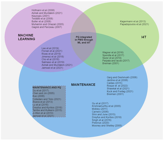
Figure 1.
Domains and references in the literature review [2,4,5,6,7,8,9,10,11,12,16,19,22,23,24,25,29,40,41,42,44,45,46,47,48,51,52,53,54,55,56,57,58,59,60,61,62,63,64,65,66,67].
According to the literature analysis, this study aims to investigate the use of ML algorithms to perform optimal PdM strategies considering PQ.
This analysis highlights the gap between the use of maintenance data through ML and the real-time control of product quality through a single framework; furthermore, appropriate PdM strategy approaches may be finalized to improve at the same time the efficiency and reliability of the manufacturing system and the PQ. These approaches should relate certain PQ features to the maintenance status of the machine and, through data collection and monitoring with I4T, dynamically define the appropriate PdM strategy.
This paper focuses on how a model integrates the key PQ variables in the PdM strategy and investigates the quality deviation that characterizes the PQ level, based on the co-effect between manufacturing system component reliability and product quality. The optimal maintenance strategy is determined by optimizing the quality cost, the repair cost, maintenance cost, and the interruption cost simultaneously, through a fuzzy real-time agent.
3. Research Methodology and Framework
Based on the existing literature, this study attempts to answer some basic questions about the connection between PdM and PQ.
The first research question aims to address the feasibility of a model that considers PQ parameters as potential variables for PdM. The basic investigation focuses on the potential relationships of machine data with predictive maintenance indicators and PQ.
RQ1: How can product quality parameters influence the problem of predictive maintenance?
The second research question aims to investigate the potential impact of PdM according to a certain level of PQ. This part of the research has been carried out by investigating the real-world ability of the model to “learn” from the PQ data and to suggest the optimal PdM.
RQ2: May we improve the MTBM and decrease maintenance and production costs through PQ optimization?
The goal of our research framework (Figure 2) is to incorporate product quality into the management of maintenance activities and to implement a suitable PdM according to a variable threshold that describes the quality level the manufacturing process must guarantee. The framework can be divided into three main steps, which provides the input variables’ definition, the predictive analysis model’s definition, and finally, validation and utilization.
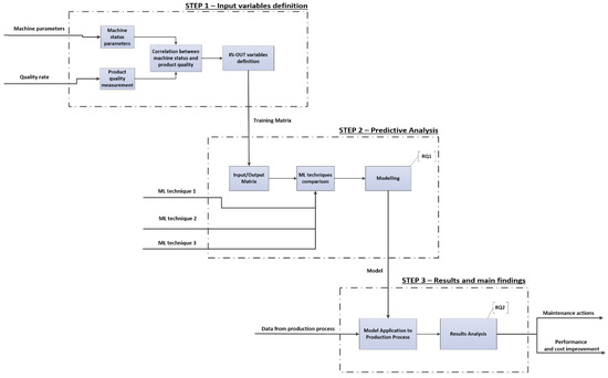
Figure 2.
Research framework.
3.1. Step 1. Input Variables’ Definition
The first step aims to define a set of variables concerning the machine status and PQ according to the application case. In this step, it is necessary to take into account the machine parameters that can be related both to the continuity of the process and the compliance of the product with the quality requirements, and to define PQ variables that follow, in a timely manner, the variations in the quality rate of the process. This step is finalized to relate the PdM to the PQ parameters or, in other words, to define which parameters will be the input and output of our model. It is important to define which parameters are important to establish the health of the machine; these can vary depending on the machines, industrial sector, or products. We can have physical parameters, such as temperature or pressure, or dynamic parameters, such as vibrations. For example, the work of Moreno et al. [68] used torque and speed as the input data to monitor the industrial system; instead, in the work of Bachraty et al. [69], the input parameters are depth of cut, cutting speed, and feed. The other important variable that we need to define is the quality variable; this one can be generally described as defected products, or can be more detailed by defining products that need to be reworked or products that are wasted. Once all variables have been defined, they are classified as input variables (if they represent machine status) or output variables (if they describe the quality rate).
3.2. Step 2. The Predictive Analysis Model’s Definition
Once the input–output data are defined, in the second step, the model structure is defined through combining the monitoring of the variables that represent the machine’s status and the prediction of the quality rate, elaborated by artificial intelligence techniques; the model will enable us to select the maintenance strategy according to the desired level of product quality. Different ML techniques are explored to build a model able to learn the behavior of the system and to detect the potential relations between the performances of the machine and the PQ parameters. In this phase, the comparison of the forecast phase, in terms of accuracy, is used between different ML techniques, each trained with the same input/output matrix defined in step 1, to validate the algorithm choice. There are many ML algorithms that can be used for this kind of system. For example, in the work of Caldas [56], the random forest algorithm is applied to the predictive maintenance of an electrical substation; Roque et al. [57] use the gradient boosting technique to perform failure detection in rotating machines through machine learning. The choice of which ML algorithm should be considered depends on the characteristics of the considered application, the available data, and the desoldered accuracy. The work of Shawkat et al. [58] proposed a new framework for learning algorithm assessment and selection, based on empirical results. Also, the work of Singh et al. [59] can be used to individuate the most interesting and suitable algorithms; it proposes a detailed review and classification of ML algorithms based on accuracy, speed of learning, complexity, and risk of over fitting measures. Finally, the work of Pistorious et al. [60] proposes a useful evaluation matrix for ML algorithm choice based on efficiency criteria, such as accuracy, model complexity, and scalability. In particular, they consider the following parameters: accuracy, training time, prediction time, resource consumption, stability, comprehensibility, scalability, complexity, and number of hyperparameters.
The final output of this step is the model that will be used to monitor the system and prevent failures.
3.3. Step 3. Validation and Results
The final step of the research framework is the application of the model in reality and the validation of the results. The input data are based on the values obtained from the process; the output includes the maintenance actions suggested by the implemented model and the impacts on the performances deriving from the process in terms of cost, maintenance parameters, and quality rate.
4. Framework Application and Case Study
In this section, the research framework was applied to a real case study. The company produces electromechanical breakers, it has 10 production lines distributed on 5 different plants, and a production capacity of about 1.3 million pcs per year.
For the application, a production line for the assembly of power transformers was chosen.
4.1. Implementation of Step 1
In this part, input variables need to be defined. The production cycle of the power transformers assembly line has the following operations (Figure 3):

Figure 3.
Production flow.
- Assembling the primary and secondary cores in the case.
- Soldering the input cable.
- Application of resin in a vacuum chamber mixer.
- Resin drying.
- Assembling the output connection.
- Insulation test.
- Functional test (check the output current).
In this manufacturing process, the vacuum mixer machine is the most critical in terms of impact on the product quality rate; the impact of this operation on the total waste generated by the manufacturing process is about 85%, while the remaining part is due to soldering (operation #2). This operation concerns the manufacture of a resin layer between the cores of the current transformer that should guarantee the electrical insulation of the product, and it is made by a vacuum mixer machine, where the working cycle is composed of three phases: loading, degassing and dosing.
During this operation, the vacuum pressure in the tanks and in the chamber is significant for the success of the phase and then for the product quality, because the vacuum casting needs to create an insulating layer without voids, bubbles, and/or porosity (Figure 4).
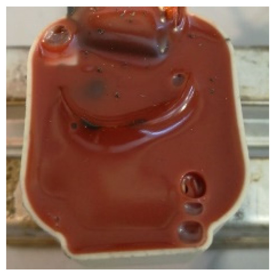
Figure 4.
Bubbles on the insulating layer.
After the final assembly, the insulation of the product is tested at a high voltage according to the customer’s specifications.
Since the product quality in our case study is related to operation #3, this study focused on the maintenance in the mixer machine that runs this operation, and specifically of the vacuum pumps (VPs) that perform the working cycle.
Vacuum pumps have the function of decreasing the pressure of a gas in a certain volume. Consequently, they must remove some gas particles from the volume.
The VPs in our mixer machine consisted of two primary parts: an electric motor and a vacuum pump. The predictive maintenance and condition monitoring of vacuum pumps is the main topic of many papers; Mooney and Shelley [61] summarize how pump predictive maintenance evolves through the use of networked monitoring systems. Konishi and Yamasawa [70] considered the issue of process by-products accumulating in the pumping system. Deposits within the pump cause friction, exceeding current limits and blocking the pump; an ARMAX model was used to predict the vacuum pump motor current. Twiddle et al. [62] tested the condition monitoring of a dry vacuum pump through a fuzzy logic scheme to identify mechanical inefficiency and exhaust system blockage through exhaust pressure. Butler et al. [63] uses artificial neural networks to estimate the degradation and RUL (remaining useful life) of the pump, using as inputs pump process data regarding all the steps in the pump cycle. Muhaimin and Ghazali [64] described a method for detecting vacuum leaks through thermography, based on IR thermography image analysis to detect leaks represented by a cold spot. Vinogradov and Kostrin [71] investigate the aspects related to oil characteristics to be monitored to establish the correct frequency of oil replacement; a visual color scale is used to determine the oil condition and maintenance action. In contrast to these results, our study used predictive maintenance as a methodology to investigate possible pump failure after the IA model predicted a deviation in product quality connected to a difference of one or more parameters with respect to the normal operating ranges of the machine.
The machine that performs operation#3 in our production cycle is equipped with 4 pumps (Figure 5):
- Resin drum pump VP1.
- Resin tank pump VP2.
- Hardener tank pump VP3.
- Dosing chamber pump VP4.
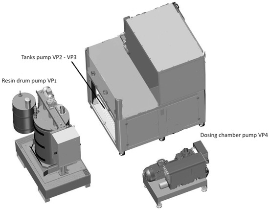
Figure 5.
Vacuum pumps in the mixer machine.
The vacuum level in the loading, degassing, and dosing phases ensures that the mixture is able to guarantee the insulation of the product. The lack of reliability of the pumps could be the cause of insufficient pressure in the tanks and in the dosing chamber, thus affecting the quality of the final product.
The pressures can be monitored by the control panel and are stored in the machine control unit. A typical maintenance indicator for vacuum pumps is the engine temperature that is stored in the machine control unit. Therefore, the parameters that allow us to define the machine’s status are pressure and temperature for each VP; the inputs of our model are presented in Table 1.

Table 1.
Machine status input variables.
The first pass yield (FPY) was chosen as the PQ variable; this index represents the percentage of pieces that do not need to be reworked, with respect to total daily production.
4.2. Implementation of Step 2
Step 2 concerns the prediction analysis, where the FPY is estimated based on the input variables, and a decision stage and a decision phase, which suggest a maintenance action based on the output of the previous stage (Figure 6).

Figure 6.
Model structure.
To choose the best ML technique to implement the predictive phase, the accuracies of a naive Bayes classifier (NBC), a nearest-neighbor classifier (NNC), and a bagged tree classifier (BTC) were compared because, from the literature review previously analyzed, it emerged that they are the most commonly used techniques for classification problems. Cakir et al. [72] compared popular ML algorithms in the design of an IoT condition-based monitoring system.
The NBC is both a supervised learning method and a statistical method for classification [73] and is used as a classifier in commercial and open source antispam e-mail filters [74]. This classification is based on the Bayes theorem and allows us to determine uncertainty by calculating probabilities of outcomes.
The NNC is a supervised learning technique used for pattern recognition [65]; this type of classifier has been used for demand forecasting production planning [66], and also as a reference system to compare other classifiers. A NNC needs, in the design stage, a set of prototype vectors, a classification rule, and a neighborhood proximity measure. The prototypes are symbolic data used by the classifier to attribute class labels. NN classification essentially consists of selecting the label of the nearest neighbor of an unknown input vector.
The bagged tree classifier (BTC) uses bagging or bootstrap aggregations to improve the variance reduction in the prediction function [75], and finds its main applications in statistical classification, predictions, and decision tree systems [76]. Random forests consist of several decision-making trees, which work as a group of de-correlated and averaged trees [67]. Averaging many noisy but roughly unbiased models allows us to reduce the variance and to use the ability of trees to capture complex interaction structures in the data.
The NBC, NNC, and BTC were trained through the MATLAB Classification Learner App with an 8 × 150 matrix input matrix and a 1 × 150 output matrix, representing the observation of 150 working days:
The pressure values of the pumps and the dosing chamber were stored on the machine control unit, the temperature values of the pumps were read by sensors and stored on the machine control unit, and the FPY index was calculated automatically by a line performance software, where operators enter data on daily production and non-compliant pieces.
The FPY output variable has been classified according to 3 categories:
- FPY < 90%.
- 90% ≤ FPY ≤ 95%.
- FPY > 95%.
Figure 7 shows the confusion matrix for the NBC trained thorough the IN and OUT matrices:
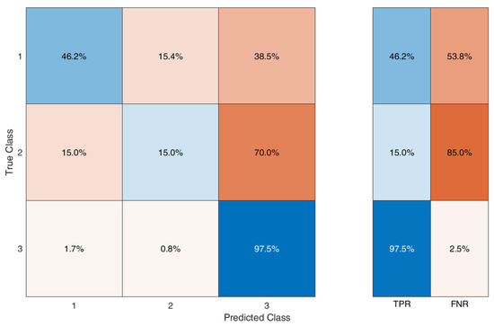
Figure 7.
Confusion matrix for the naive Bayes classifier.
In this case, the FNR is high for classes 1 and 2 (representing, respectively, FPY = 2 and FPY = 1). This indicates that the naive Bayes classifier should not predict the correct output when the input variables should suggest an FPY index in these two classes.
In the scatter plot (p4 vs. t4) in Figure 8, the yellow, orange, and blue dots represent, respectively, FPY = 1, FPY = 2, and FPY = 3. In addition, the yellow and orange dots overlap in some areas of the plot (X represents incorrect predictions).
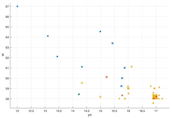
Figure 8.
Scatter plot for the naive Bayes classifier (p4 vs. t4).
This indicates the NNC is unable to predict the right output. The overall accuracy for the NBC is 75%.
Figure 9 shows the confusion matrix for an NNC (K = 1) trained with IN and OUT matrices.
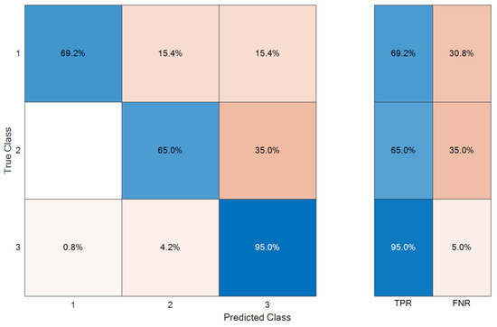
Figure 9.
Confusion matrix for the nearest neighbor classifier.
In this case, the FNR is better for classes 1 and 2 (representing, respectively, FPY = 2 and FPY = 1), but the accuracy is lower in the prediction of class 3; the scatter plot (Figure 10) shows overlapping for classes 1 and 2.
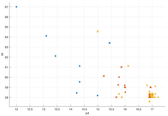
Figure 10.
Scatter plot for the nearest neighbor classifier (p4 vs. t4).
The overall accuracy for the NNC is 88%.
For the BTC, the best accuracy result (91%) was obtained, with 30 as the number of learners (the number of decision trees in the random forest) and 151 splits (the depth of the decision tree); Figure 11 displays the confusion matrix for the BTC.
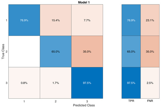
Figure 11.
Confusion matrix for the bagged tree classifier.
In this case, the FNR is better for class 3 with respect to the NBC and NNC.
The scatter plot (Figure 12) shows overlapping for classes 1 and 2, and displays the confusion matrix for the BTC.
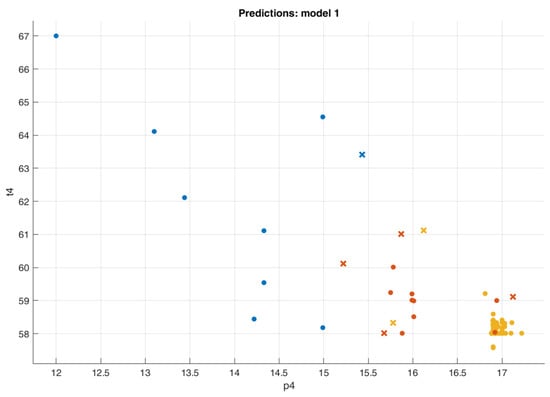
Figure 12.
Scatter plot for the bagged tree classifier (p4 vs. t4).
We compared the overall accuracy of the naive Bayes classifier and nearest neighbor classifier with that of the BTC (Table 2).

Table 2.
Accuracy comparison among ML techniques.
The latter was chosen as the predictor of our model.
The predictive phase was completed by combining the bagged tree classifier (BTC) with a fuzzy inference engine (FIE). Variables that describe the state of the machine were used as the inputs of the BTC and FIE, and the predicted FPY (BTC output) represents an additional input to the FIE to determine the appropriate maintenance action for each pump (Figure 13).
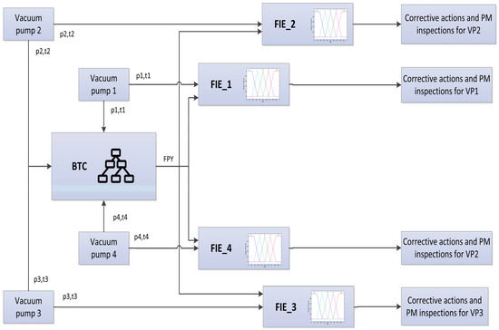
Figure 13.
Model flow.
In summary, the BTC elaborates a prediction, based on the machine status, of the quality rate of the process, and the FIE suggests which corrective action should be carried out on the process according to the BTC output and to the machine status parameters. This strategy uses the BTC to predict the behavior of the system and the objectivity of the fuzzy rules to decide the action to be taken [77].
In more detail, the FIE receives as an input normalized the pressure and temperature of each VP the and normalized FPY level estimated by the BTC, and elaborates a criticality index IC according to a set of rules (Figure 14).

Figure 14.
FIE flow.
The rules are designed to assess whether FPY index deviation is caused by human error or an actual anomaly in the pump. In the first case, a low-pressure value (VL), not corresponding to an increase in temperature (L), and an FPY = 2 (M) indicate a setup error (IC = M), as expressed by the following rule:
if (Pressure is VL) and (Temperature is L) and (FPY is M) then (Ic is M)
In the second case, the pressure drop combined with a high temperature (VH), and an FPY = 1, leads to a high IC (H):
if (Pressure is VL) and (Temperature is VH) and (FPY is L) then (Ic is H)
Through the index value, a corrective action (after defuzzification) is suggested to the user as follows:
- IC = L → no action.
- IC = M → setup error—check the pump’s setup.
- IC = H → possible engine failure—check the temperature in the vacuum pump’s engine).
This portion of the study responds to the need, expressed through RQ1, to include the quality parameters of the product within the problem of predictive maintenance. In fact, the prediction of the FPY is used, together with the operating parameters of the machine, as one of the variables that guides the decision of the model with respect to the choice of maintenance actions.
4.3. Implementation of Step 3
In step 3, we analyze how the model predicts the quality rate and suggests a maintenance action through 3 different cases:
- The parameters of all VPs are in the normal operating range:In this case, no action is required on VP1, VP2, VP3, or VP4.
- The pressure of VP4 is low:In this case, the FIE suggests checking the pressure setup of VP4 (the low pressure may be caused by an operator error).
- The pressure of VP4 is low and the temperature is high:
The FIE considers the association between the pressure drop and the temperature increase as an anomaly that causes the failure of the pump; the suggested action is to inspect the overheated area with a thermographic camera (Figure 15).
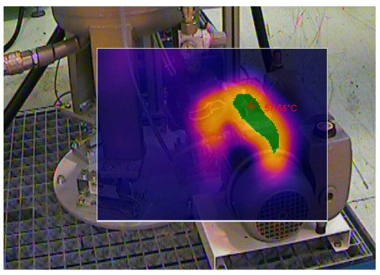
Figure 15.
Thermographic inspection of a VP.
In case 1, the model evaluates the input data as an optimal situation; in case 2 the low pressure, not being correlated to an increase in engine temperature, is judged as a setup error by the operator. In case 3, the temperature increase is considered as a signal of a possible pump failure.
The model was applied to the manufacturing process for a period of 6 months, corresponding to an observation period of 150 working days, each with two shifts.
During this period, 46 anomalies were detected in the 4 vacuum pumps, of which 32 were considered to be resolved with checking the machine parameters, and 14 were evaluated as possible pump failures.
Table 3 shows the difference between real events and the predicted events in the 2 categories of anomalies.

Table 3.
Real events vs. predicted events.
In summary, 96.9% of setup errors were correctly predicted by the model, and 92.8% of possible failures were reported and confirmed by a thermographic inspection of the vacuum pump. In one case, failure was not even predicted (with serious damage to the pump), because the anomaly had not generated an increase in temperature, and consequently the model was not able to anticipate failure.
An interesting result concerns the variations in MTBF and FPY by comparing the “before PdM” data and the period of the first application of the model to the manufacturing process, i.e., “after PdM”. Table 4 shows the results and benefits, referring to a period of 150 days, in terms of number of maintenance events (NMEs), MTBM, MTTR, availability A, and FPY, where the MTBM is calculated as [78] in (3):
and availability as in (4):

Table 4.
Process parameters during data collection and model application.
The comparison shows an evident improvement in the MTBM (from 37.8 to 48.6 h) (Figure 16).
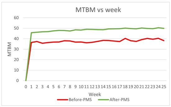
Figure 16.
MTBM comparison between data collection and model application.
At the same time, the optimization of the FPY index (Figure 17) confirms that the inclusion in the model of a production quality index, which must be monitored and optimized, effectively leads to an improvement in the continuity of operation of the machine (availability increases from 93.1% to 96.6%), when this index is dependent on some operating parameters of the machine itself (RQ2).
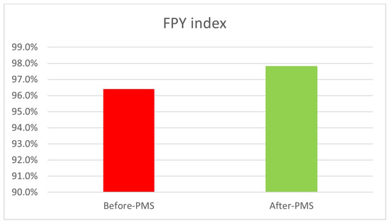
Figure 17.
FPY comparison between As-Is phase and model application.
Calculated as [78] in (1): the naive Bayes classifier and nearest neighbor classifier.
5. Cost Analysis
Finally, this section aims to evaluate the costs that can be reduced by the application of a PdM model considering PQ. The total cost of the situation before the framework’s application is calculated in the case study and compared with the result achieved after the framework’s application. The total cost, , is calculated as the sum of cost related to the lack of production during machine downtime, ; the cost of maintenance interventions, ; the cost of the time necessary for the reworking of waste pieces, ; and the cost related to the implementation of the AI model, , in a certain period, T (usually one year), as expressed in (5):
The “Cost of Downtime ()” is expressed as:
where K1 is the missed production hourly cost, NME corresponds to the number of maintenance events in the considered period, T, and the MTTR parameter is the mean time to repair (Table 5).

Table 5.
Data for cost calculation.
Maintenance cost is calculated as the number of maintenance events that happened in the considered period multiplied by the average maintenance hourly cost (K2), the MTTR, and the average cost of spare parts, , multiplied by the number of maintenance events in the considered period.
The scraps cost is evaluated as:
where K3 is the manual labor hourly cost, V is the production during the considered period, FPY is defined as the “First Pass Yield First Pass Yield”, i.e., the percentage of pieces that don not need to be reworked, and finally, RWT is the reworking time needed for each piece.
Finally, the “Cost of Implementation ()” is:
where K4 is the depreciation cost for the implementation of the model (sensors, software, thermographic tools, etc.) and K5 is the managing cost of the tools referring to the considered period, T.
Cost evaluation is applied to the case study, and Table 5 summarizes the used data referring to the observation period of T = 150 days.
In Table 6, the costs of the data collection phase and the period of first application of the model to the manufacturing process are reported (T = 150 days).

Table 6.
Cost comparison between “Before PdM” and “After PdM”.
The application of the model to the manufacturing process allows us to save about 50% of the cost for machine stops and 64% of costs for scraps (Figure 18).
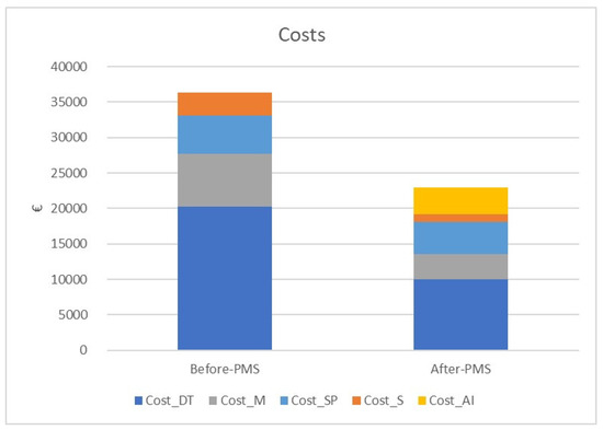
Figure 18.
Cost comparison between data collection and model application.
6. Discussion
The application of the framework to a real case study demonstrates the utility of linking the PQ parameter to the PdM definition using ML models. The results show the benefits not only in terms of time and performance, as the MTBM and the FYP increase by about 28.6% and 2.3%, respectively, but also the economic ones in terms of saving about 37% less of the total cost. Also, the operating time and the NME improve, the MTTR decreases by about 40%, and the overall availability increases from 93.1% to 96.6%. The first step, i.e., the data collection, is the most time consuming, if I4Ts are not implemented yet. After that, the choice of the ML algorithm and the model construction depends on the criticalities of the system.
The application of the model to the production line of electromechanical components allows us to respond to the RQs:
- RQ1: the relation of machines’ data to predictive maintenance indicators and PQ is implemented through a prediction stage of the quality rate based on the machine variables and a “decisional” stage through fuzzy logic;
- RQ2: the link between the variables that describe the status of the machine and the qualitative rate of the manufacturing process allows us to control maintenance actions based on scraps optimization, achieving an improvement in the operation of the machine. Moreover, this results in an estimated saving of about 50% of the costs for machine downtime and 64% of the costs for scraps.
To verify that the developed framework is of general application, it was also tested on a different production process; specifically, how it worked on a CNC turning process was verified.
According to the results of the study by [79], one of the machine parameters that can affect the quality of the final product (in terms of dimensions and surface roughness) is the cutting speed; based on the results of the experiments reported in this research, variations in the cutting speed impact the heat gradient between the tool and raw material, causing dimensional and roughness variations in the product.
The emulsion system of CNC lathes has the function of delivering cutting oil to the tools to avoid overheating and control tool wear; this system, however, is also one of the components most vulnerable to failures in this type of machines [80].
Based on these considerations, the model has been trained with a matrix, built through 150 working shifts of observation, which has as input variables the cutting speeds SC and TC (expressed as percentage override [0–150%]) and the temperature in the cutting chamber, and as output the FPY rate, classified according to three categories:
- FPY < 50%.
- 50% ≤ FPY ≤ 90%.
- FPY > 90%.
Also, in this application, the model predicts the quality rate and suggests a maintenance action through three different cases:
SC and TC are in the normal range:
SC and TC are high:
TC is high:
This second application shows how the framework works correctly on a different production process, after having trained the system with a matrix in which the input variables are the system parameters that directly impact the quality of the final product.
The use of the model on the turning process was carried out for a period of 6 weeks on five machines, with the results shown in Table 7.

Table 7.
Results of model application to turning process.
Preliminary data show a link between the number of anomalies found in the emulsion system and the decrease in FPY, in particular for machine 3 (which has the highest number of working hours); however, the link between machine performance, product geometry, and the type of material processed should be investigated with more data, and it should be taken into account that the machines have different characteristics (speed, bar channel, and control module). The analysis must also be completed with the evaluation of the costs.
7. Conclusions and Further Research
Predictive maintenance is of course a strategic tool to optimize production, reducing the machine’s downtime and scraps. With respect to preventive maintenance, it allowed us to maximize the RUL of components through the continuous monitoring of the production system’s behavior, reducing not only the failures, but also unnecessary maintenance activities. The high use of I4T in industries has made it possible to considerably improve PdM applications, making available a large amount of data that can be used as the input for AI. AI, with the application of different ML algorithms, is a novel and successful tool applied in PdM. An important parameter that can be considered for maintenance prediction is the quality of the product. In fact, machines can continue to work without failures, but produce more and more scraps; this can be a signal of an imminent failure.
To combine the PQ parameter and PdM, this study proposed a new framework, with the aim of guiding practitioners and the research on this issue. According to the results of the literature review, the novelty of the approach adopted in this framework is the possibility of managing the process performance in an integrated way, both in terms of the number and duration of stops and quantity of waste pieces. The identification of a link between the state of the machine and the quality of the pieces produced makes it possible, through the use of ML techniques, to obtain a combined improvement in production continuity and the quality rate, with savings on the overall costs of the production process. The framework has been applied to a real case study and a costs analysis has been carried out.
The results are encouraging, as it is possible to obtain an indication of the predictive maintenance action to anticipate possible failures related to the state of the machine and the production quality rate, and achieve a saving of about 37% of actual costs.
The application of the model to the production line leads to the assertion that, when there is a link between the variables that describe the operating status of the machine and the qualitative parameters of the production process, it is possible to control maintenance actions on the basis of the optimization of waste, obtaining, at the same time, an improvement in the operation of the machine and cost optimization.
In the Industry 4.0 context, the model can be used as a tool to improve the maturity of the company in data collection and data handling. In fact, the model requires collecting data in a structured way, identifying critical components, and, through data analysis, basing decisions on the data. So, according to the classification presented in [81], this scenario represents an intermediate level of maturity for data handling and allows one to jump to an advanced level if the continuous improvement loop is implemented.
7.1. Managerial Implications
This research resulted from industrial activities aimed at developing a framework for the management of maintenance activities in relation to quality targets. The model has been developed through ML to support maintenance manager and production manager in planning of maintenance actions according to the real-time monitoring of machine parameters and a prediction of quality rate, with the goals of guaranteeing the continuity of production flow and a low percentage of not-compliant pieces.
From a managerial perspective, this study and its activities have addressed the mutual effect of machine performances and quality requirements based on the process data, supporting the company in evaluating the impact of maintenance costs and quality costs within a single framework. This is not mandatory but may be added if there are patents resulting from the work reported in this manuscript.
7.2. Future Research
Future research will address the following points:
- The use of additional machine variables that make the prediction of failures more accurate and can exploit, with a continuous improvement loop, the knowledge generated by the analysis of maintenance interventions data.
- The use of ML in step 1 of the research framework as a tool to detect the correlation between machine parameters and the quality rate of the process.
- The inclusion in the comparison with other ML techniques and an analysis of how the configuration parameters of these techniques affect the behavior of the model in terms of prediction accuracy.
- The introduction of a second output variable representing the product’s performance in the prediction stage.
- The application of the framework to different types of production processes.
- Comparison of the accuracy of the prediction phase considering the use of the fast Fourier transform (FFT).
Author Contributions
Conceptualization, C.R. and M.M.; Methodology, C.R., M.M. and I.Z.; Software, C.R. and M.M.; Validation, C.R., M.M. and I.Z.; Formal analysis, C.R., M.M. and I.Z.; Investigation, C.R. and M.M.; Resources, C.R., M.M. and I.Z.; Data curation, C.R. and M.M.; Writing—original draft preparation, C.R. and M.M.; Writing—review and editing, I.Z. and M.M.S.; Supervision, I.Z. and M.M.S. All authors have read and agreed to the published version of the manuscript.
Funding
This research received no external funding.
Data Availability Statement
The raw data supporting the conclusions of this article will be made available by the authors on request.
Conflicts of Interest
The authors declare no conflicts of interest.
Nomenclature
| Abbreviation | Description |
| PdM | Predictive Maintenance |
| ML | Machine Learning |
| PQ | Product Quality |
| I4Ts | Industry 4.0 Technologies |
| PMSs | Predictive Maintenance Strategies |
| MTBM | Mean Time Between Maintenance |
| AI | Artificial Intelligence |
| RUL | Remaining Useful Life |
| RFID | Radio-Frequency IDentification |
| MEMS | Micro-Electro-Mechanical System |
| PEIDs | Product Embedded Information Devices |
| SA | Simulated Annealing |
| GA | Genetic Algorithm |
| VPs | Vacuum Pumps |
| FPY | First Pass Yield |
| NBC | Naive Bayes Classifier |
| NNC | Nearest Neighbour Classifier |
| BTC | Bagged Tree Classifier |
| FIE | Fuzzy Inference Engine |
| NMEs | Number of maintenance events |
| Total cost | |
| Machine downtime | |
| Cost of maintenance interventions | |
| Scraps cost | |
| Cost related to the implementation of the AI model | |
| Cost of downtime | |
| Cost of spare parts | |
| K1 | Average missed production hourly cost |
| K2 | Average maintenance hourly cost |
| K3 | Average manpower hourly cost |
| K4 | Implementation cost |
| K5 | Managing cost of the tools |
| V | Production volume |
| RWT | Reworking time |
| MTTR | Mean time between repair |
References
- Bouslah, B.; Gharbi, A.; Pellerin, R. Joint production, quality and maintenance control of a two-machine line subject to operation-dependent and quality-dependent failures. Int. J. Prod. Econ. 2018, 195, 210–226. [Google Scholar] [CrossRef]
- Garg, A.; Deshmukh, S.G. Maintenance management: Literature review and directions. J. Qual. Maint. Eng. 2006, 12, 205–238. [Google Scholar] [CrossRef]
- Faccio, M.; Persona, A.; Sgarbossa, F. Industrial maintenance policy development: A quantitative framework. Int. J. Prod. Econ. 2014, 147 Pt A, 85–93. [Google Scholar] [CrossRef]
- Kagermann, H.; Wahlster, W.; Helbig, J. Recommendations for Implementing the Strategic Initiative Industrie 4.0; Acatech National Academy of Science and Engineering: Frankfurt, Germany, 2013. [Google Scholar]
- Papadopoulos, T.; Singh, S.P.; Spanaki, K.; Gunasekaran, A.; Dubey, R. Towards the next Generation of Manufacturing: Implications of Big Data and Digitalization in the Context of Industry 4.0. Prod. Plan. Control 2021, 33, 101–104. [Google Scholar] [CrossRef]
- Lee, W.J.; Wu, H.; Yun, H.; Kim, H.; Jun, M.B.; Sutherland, J.W. Predictive maintenance of machine tool systems using artificial intelligence techniques applied to machine condition data. Procedia CIRP 2019, 80, 506–511. [Google Scholar] [CrossRef]
- Gu, C.; He, Y.; Han, X.; Chen, Z. Product quality oriented predictive maintenance strategy for manufacturing systems. In Proceedings of the IEEE Prognostics and System Health Management Conference, Harbin, China, 9–12 July 2017. [Google Scholar]
- Chen, Y.; Jin, J. Quality-reliability chain modeling for system-reliability analysis of complex manufacturing processes. IEEE Trans. Reliab. 2005, 54, 475–488. [Google Scholar] [CrossRef]
- Florian, E.; Sgarbossa, F.; Zennaro, I. Machine learning-based predictive maintenance: A cost-oriented model for implementation. Int. J. Prod. Econ. 2021, 236, 108114. [Google Scholar] [CrossRef]
- Krishnamurthy, L.; Adler, R.; Buonadonna, P.; Chhabra, J.; Flanigan, M.; Kushalnagar, N.; Nachman, L.; Yarvis, M. Design and deployment of industrial sensor networks: Experiences from a semiconductor plant and the North Sea. In Proceedings of the 3rd International Conference on Embedded Networked Sensor Systems, San Diego, CA, USA, 2–4 November 2005; pp. 64–75. [Google Scholar]
- Mobley, R.K. Maintenance Fundamentals, 2nd ed.; Butterworth-Heinemann: Oxford, UK, 2011. [Google Scholar]
- Carnero, M.C. An evaluation system of the setting up of predictive maintenance programmes. Reliab. Eng. Syst. Saf. 2006, 91, 945–963. [Google Scholar] [CrossRef]
- Wu, D.; Jennings, C.; Terpenny, J.; Gao, R.X.; Kumara, S. A comparative study on machine learning algorithms for smart manufacturing: Tool wear prediction using random forests. J. Manuf. Sci. Eng. 2017, 139, 071018. [Google Scholar] [CrossRef]
- Paolanti, M.; Romeo, L.; Felicetti, A.; Mancini, A.; Frontoni, E.; Loncarski, J. Machine Learning approach for Predictive Maintenance in Industry 4.0. In Proceedings of the 14th IEEE/ASME International Conference on Mechatronic and Embedded Systems and Applications (MESA), Oulu, Finland, 2–4 July 2018. [Google Scholar]
- Martin, K.F. A review by discussion of condition monitoring and fault diagnosis in machine tools. Int. J. Mach. Tools Manuf. 1994, 34, 527–551. [Google Scholar] [CrossRef]
- Jardine, A.K.S.; Lin, D.; Banjevic, D. A review on machinery diagnostics and prognostics implementing condition-based maintenance. Mech. Syst. Signal Process. 2006, 20, 1483–1510. [Google Scholar] [CrossRef]
- Jang, Y.J.; Dai, P.; Fang, P.; Zhong, R.Y.; Zhao, X. A2-LSTM for predictive maintenance of industrial equipment based on machine learning. Comput. Ind. Eng. 2022, 172, 108560. [Google Scholar] [CrossRef]
- Rosati, R.; Romeo, L.; Cecchini, L.; Tonetto, F.; Viti, P.; Mancini, A.; Frontoni, F. From knowledge-based to big data analytic model: A novel IoT and machine learning based decision support system for predictive maintenance in Industry 4.0. J. Intell. Manuf. 2022, 34, 107–121. [Google Scholar] [CrossRef]
- Hofmann, T.; Schölkopf, B.; Smola, A.J. Kernel methods in machine learning. Ann. Stat. 2008, 36, 1171–1220. [Google Scholar] [CrossRef]
- Wagner, C.; Saalmann, P.; Hellingrath, B. An Overview of Useful Data and Analysing Techniques for Improved Multivariate Diagnostics and Prognostics in Condition-Based MaintenanceProce. In Proceedings of the Annual Conference of the Prognostics and Health Management Society, Denver, CO, USA, 3–6 October 2016; pp. 183–191. [Google Scholar]
- Romeo, L.; Loncarski, J.; Paolanti, M.; Bocchini, G.; Mancini, A.; Frontoni, E. Machine learning-based design support system for the prediction of heterogeneous machine parameters in industry 4.0. Expert Syst. Appl. 2020, 140, 112869. [Google Scholar] [CrossRef]
- Rivas, A.; Jesus, M.; Fraile, J.M.; Chamoso, P.; Gonzalez-Briones, A.; Sitton, I.; Corchado, J.M. A Predictive Maintenance Model Using Recurrent Neural Networks. In Proceedings of the 14th International Conference on Soft Computing Models in Industrial and Environmental Applications, Seville, Spain, 13–15 May 2019; pp. 261–270. [Google Scholar]
- Jimenez, A.A.; Gómez Muñoz, C.Q.; García Márquez, F.P. Machine Learning and Neural Network for Maintenance Management. In Proceedings of the International Conference on Management Science and Engineering Management, Melbourne, VIC, Australia, 1–4 August 2018. [Google Scholar]
- Cho, S.; May, G.; Tourkogiorgis, I.; Perez, R.; Lazaro, O.; de la Maza, B.; Kiritsis, D. A Hybrid Machine Learning Approach for Predictive Maintenance in Smart Factories of the Future. In Proceedings of the IFIP International Federation for Information Processing, Poznan, Poland, 17–21 September 2018; pp. 311–317. [Google Scholar]
- Salmaso, L.; Pegoraro, L.; Giancristofaro, R.; Ceccato, R.; Bianchi, A.; Restello, S.; Scarabottolo, D. Design of experiments and machine learning to improve robustness of predictive maintenance with application to a real case study. Commun. Stat.—Simul. Comput. 2019, 51, 1–13. [Google Scholar] [CrossRef]
- Lamban, M.J.; Morella, P.; Royo, J.; Sanchez, J.C. Using industry 4.0 to face the challenges of predictive maintenance: A key performance indicators development in a cyber physical system. Comput. Ind. Eng. 2022, 171, 108400. [Google Scholar] [CrossRef]
- Tortorella, G.L.; Fogliatto, F.S.; Cauchick-Miguel, P.A.; Kurnia, S.; Jurburg, D. Integration of Industry 4.0 technologies into Total Productive Maintenance practices. Int. J. Prod. Econ. 2021, 240, 108224. [Google Scholar] [CrossRef]
- Carvalho, T.P.; Soares, F.; Vita, R.; Francisco, R.; Basto, J.P.; Alcala, S.G. A systematic literature review of machine learning methods applied to predictive maintenance. Comput. Ind. Eng. 2019, 137, 106024. [Google Scholar] [CrossRef]
- Shin, J.H.; Jun, H.B. On condition-based maintenance policy. J. Comput. Des. Eng. 2015, 2, 119–127. [Google Scholar] [CrossRef]
- De Jesus Pacheco, P.A.; Jung, C.F.; De Azambuja, M.C. Towards industry 4.0 in practice: A novel RFID-based intelligent system for monitoring and optimisation of production systems. J. Intell. Manuf. 2021, 34, 1165–1181. [Google Scholar] [CrossRef]
- Prajapati, A.; Betchel, J.; Ganesan, S. Condition based maintenance: A survey. J. Qual. Maint. Eng. 2012, 18, 384–400. [Google Scholar] [CrossRef]
- Kobbacy, K.A.H.; Prabhakar Murthy, D.N. Complex System Maintenance Handbook; Springer Series in Reliability Engineering; Springer: Berlin/Heidelberg, Germany, 2008. [Google Scholar]
- Paolanti, M.; Frontoni, E.; Mancini, A.; Pierdicca, R.; Zingretti, P. Automatic Classification for Anti Mixup Events in Advanced Manufacturing System. In Proceedings of the ASME International Design Engineering Technical Conferences and Computers and Information in Engineering Conference, Boston, MA, USA, 2–5 August 2015. [Google Scholar]
- Wang, X.; Wang, H.; Qi, C. Multi-agent reinforcement learning based maintenance policy for a resource constrained flow line system. J. Intell. Manuf. 2016, 27, 325–333. [Google Scholar] [CrossRef]
- Susto, G.A.; Schirru, A.; Pampuri, S.; McLoone, S. Supervised Aggregative Feature Extraction for Big Data Time Series Regression. IEEE Trans. Ind. Inform. 2016, 12, 3. [Google Scholar] [CrossRef]
- Naspetti, S.; Pierdicca, R.; Mandolesi, S.; Paolanti, M.; Frontoni, E.; Zanoli, R. Automatic Analysis of Eye-Tracking Data for Augmented Reality Applications: A Prospective Outlook. In Lecture Notes in Computer Science; Springer International Publishing: Berlin/Heidelberg, Germany, 2016; p. 9769. [Google Scholar]
- Druck, G.; Mann, G.; McCallum, A. Learning from Labeled Features using Generalized Expectation Criteria. In Proceedings of the 31st Annual International ACM SIGIR Conference on Research and Development in Information Retrieval, Singapore, 20–24 July 2008; pp. 595–602. [Google Scholar]
- Heng, A.; Tan, A.C.C.; Mathew, J.; Montgomery, N.; Banjevic, D.; Jardine, A.K.S. Intelligent condition-based prediction of machinery reliability. Mech. Syst. Signal Process. 2009, 23, 1600–1614. [Google Scholar] [CrossRef]
- Su, Y.C.; Cheng, F.T.; Hung, M.H.; Huang, H.C. Intelligent Prognostics System Design and Implementation. IEEE Trans. Semicond. Manuf. 2006, 19, 195–207. [Google Scholar] [CrossRef]
- Kuo, Y. Optimal adaptive control policy for joint machine maintenance and product quality control. Eur. J. Oper. Res. 2006, 171, 586–597. [Google Scholar] [CrossRef]
- Colledani, M.; Tolio, T. Integrated quality, production logistics and maintenance analysis of multi-stage asynchronous manufacturing systems with degrading machines. CIRP Ann. 2021, 61, 455–458. [Google Scholar] [CrossRef]
- Rivera-Gómez, H.; Gharbi, A.; Kenné, J.P. Joint production and major maintenance planning policy of a manufacturing system with deteriorating quality. Int. J. Prod. Econ. 2013, 146, 575–587. [Google Scholar] [CrossRef]
- Ait-El-Kadi, A.; Gharbi, A.; Dhouib, K.; Artiba, A. Integrated production, maintenance and quality control policy for unreliable manufacturing systems under dynamic inspection. Int. J. Prod. Econ. 2021, 236, 108140. [Google Scholar] [CrossRef]
- Lu, B.; Zhou, X.; Li, Y. Joint modelling of preventive maintenance and quality improvement for deteriorating single-machine manufacturing systems. Comput. Ind. Eng. 2016, 91, 188–196. [Google Scholar] [CrossRef]
- Dreyfus, P.A.; Kyritsis, D. A Framework Based on Predictive Maintenance, Zero-Defect Manufacturing and Scheduling under Uncertainty Tools, to Optimize Production Capacities of High-End Quality Products. In Proceedings of the IFIP International Federation for Information Processing, Poznan, Poland, 18–19 September 2018; pp. 296–303. [Google Scholar]
- Tambe, P.P.; Kulkarni, M.S. A superimposition-based approach for maintenance and quality plan optimization with production schedule, availability, repair time and detection time constraints for a single machine. J. Manuf. Syst. 2015, 37, 17–32. [Google Scholar] [CrossRef]
- Spendla, L.; Kebisek, M.; Tanuska, P.; Hrcka, L. Concept of Predictive Maintenance of Production Systems in Accordance with Industry 4.0. In Proceedings of the IEEE 15th International Symposium on Applied Machine Intelligence and Informatics (SAMI), Herl’any, Slovakia, 26–28 January 2017; pp. 405–410. [Google Scholar]
- Sezer, E.; David Romero, D.; Guedeal, F.; Macchi, M.; Emmanouilidis, C. An Industry 4.0-enabled Low-Cost Predictive Maintenance Approach for SMEs: A Use Case Applied to a CNC Turning Centre. In Proceedings of the IEEE International Conference on Engineering, Technology and Innovation (ICE/ITMC), Stuttgart, Germany, 17–20 June 2018. [Google Scholar]
- Zhou, B.; Pychynski, T.; Reischl, M.; Kharlamov, E.; Mikut, R. Machine learning with domain knowledge for predictive quality monitoring in resistance spot welding. J. Intell. Manuf. 2022, 33, 1139–1163. [Google Scholar] [CrossRef]
- Tercan, H.; Meisen, T. Machine learning and deep learning based predictive quality in manufacturing: A systematic review. J. Intell. Manuf. 2022, 33, 1879–1905. [Google Scholar] [CrossRef]
- Ashek-Al-Aziz, M.; Muntakim, A.H. No relationship between rate of learning and other parameters of Neural Network—A Matlab experience. J. Multidiscip. Eng. Sci. Technol. 2021, 8. [Google Scholar]
- Kayzoglu, T. An Investigation of the Design and Use of Feed forward Artificial Neural Networks in the Classification of Remotely Sensed Images. Ph.D. Thesis, University of Nottingham, Nottingham, UK, 2001. [Google Scholar]
- Sun, J.-W.; Xi, L.-F.; Du, S.-C.; Pan, E.-S. Tool maintenance optimization for multi-station machining systems with economic consideration of quality loss and obsolescence. Robot. Comput.-Integr. Manuf. 2010, 26, 145–155. [Google Scholar]
- Jamwal, A.; Agrawal, R.; Sharma, M.; Kumar, A.; Kumar, V.; Garza-Reyes, J.A.A. Machine Learning Applications for Sustainable Manufacturing: A Bibliometric-Based Review for Future Research. J. Enterp. Inf. Manag. 2021, 35, 566–596. [Google Scholar] [CrossRef]
- Parpala, R.C.; Iacob, R. Application of IoT concept on predictive maintenance of industrial equipment. MATEC Web Conf. 2017, 121, 02008. [Google Scholar] [CrossRef]
- Caldas, A.N. Desenvolvimento de um Sistema de Apoio à Decisao Para a Manutencao Preditiva dos Ativos de Uma Subestacao Eletrica. Master’s Thesis, Faculdade de Engenharia, Universidade do Porto, FEUP, Porto, Portugal, 2015. [Google Scholar]
- Roque, A.S.; Krebs, V.W.; Figueiro, I.C.; Nasser Jazdi, N. An analysis of machine learning algorithms in rotating machines maintenance. IFAC-PapersOnLine 2022, 55, 252–257. [Google Scholar] [CrossRef]
- Shawkat, M.; Bin Risal, A.R.; Mahdi, N.J.; Safari, Z.; Naser, M.H.; Al Zand, A.W. Fluid Flow Behavior Prediction in Naturally Fractured Reservoirs Using Machine Learning Models. Technol.-Based Adv. Mach. Learn. Models Appl. Civ. Eng. 2021, 23, 7953967. [Google Scholar] [CrossRef]
- Singh, A.; Thakur, N.; Sharma, A. A review of supervised machine learning algorithms. In Proceedings of the 3rd International Conference on Computing for Sustainable Global Development, New Delhi, India, 16–18 March 2016; pp. 1310–1315. [Google Scholar]
- Pistorius, F.; Grimm, D.; Erdösi, F.; Sax, E. Evaluation matrix for smart machine-learning algorithm choice. In Proceedings of the IEEE 1st International Conference on Big Data Analytics and Practices (IBDAP), Bangkok, Thailand, 25–26 September 2020; pp. 1–6. [Google Scholar]
- Mooney, M.; Shelley, G. Data collection and networking capabilities enable pump predictive diagnostic. Solid State Technol. 2005, 48, 49–63. [Google Scholar]
- Twiddle, A.; Jone, N.B.; Spurgeon, S.K. Fuzzy model-based condition monitoring of a dry vacuum pump via time and frequency analysis of the exhaust pressure signal. Proc. Inst. Mech. Eng. Part C J. Mech. Eng. Sci. 2008, 222, 287–293. [Google Scholar] [CrossRef]
- Butler, S.W.; Ringwood, J.V.; MacGearailt, N. Prediction of Vacuum Pump Degradation in Semiconductor Processing. In Proceedings of the 7th IFAC Symposium on Fault Detection, Supervision and Safety of Technical Processes, Barcelona, Spain, 30 June–3 July 2009. [Google Scholar]
- Muhaimin, M.N.; Ghazali, K.H. IR thermography application for vacuum leak detection of absorption chiller in petrochemical plant. ARPN J. Eng. Appl. Sci. 2015, 10, 10686–10690. [Google Scholar]
- Gagné, C.; Parizeau, M. Coevolution of nearest neighbor classifiers. Int. J. Pattern Recognit. Artif. Intell. 2007, 21, 921–946. [Google Scholar] [CrossRef]
- Kuck, M.; Freitag, M. Forecasting of customer demands for production planning by local k-nearest neighbor models. Int. J. Prod. Econ. 2021, 231, 107837. [Google Scholar] [CrossRef]
- Breiman, L. Random Forests. Mach. Learn. 2001, 45, 5–32. [Google Scholar] [CrossRef]
- Moreno, R.; Pintado, P.; Chicharro, J.M.; Morales, A.L.; Nieto, A.J. Methodology for evaluating neural networks inputs for gear fault detection. In Proceedings of the 2009 IEEE International Conference on Mechatronics, Málaga, Spain, 14–17 April 2009. [Google Scholar]
- Bachratya, M.; Tolnaya, M.; Kovacb, P.; Pucovsky, V. Neural Network Modeling of Cutting Fluid Impact on Energy Consumption during Turning. Tribol. Ind. 2016, 38, 149–155. [Google Scholar]
- Konishi, S.; Yamasawa, K. Diagnostic system to determine the in-service life of dry vacuum pumps. In Proceedings of the IEEE Proceedings—Science, Measurement and Technology, San Juan, Puerto Rico, 10–13 November 1999; Volume 146, pp. 270–276. [Google Scholar]
- Vinogradov, M.L.; Kostrin, D.K. Characteristics, Rules of Replacement and Operation of Vacuum Pump Oils. AIP Conf. Proc. 2019, 2089, 020021. [Google Scholar]
- Cakir, M.J.; Guvenc, M.A.; Mistikoglu, S. The experimental application of popular machine learning algorithms on predictive maintenance and the design of IoT based condition monitoring system. Comput. Ind. Eng. 2021, 151, 106948. [Google Scholar] [CrossRef]
- Vijaykumar, B.; Vikramkumar, T. Bayes and naive-bayes classifier. arXiv 2014, arXiv:1404.0933. [Google Scholar]
- Metsis, V.; Androutsopoulos, I.; Paliouras, G. Spam filtering with naive bayes-which naive bayes? CEAS 2006, 17, 28–69. [Google Scholar]
- Hastie, T.; Tibshirani, R.; Friedman, J. The Elements of Statistical Learning; Springer Series in Statistics; Springer: Berlin/Heidelberg, Germany, 2009; pp. 587–604. [Google Scholar]
- Purnachand, K.; Shabbeer, M.; Rao, P.N.V.S.; Madhu Babu, C. Predictive Maintenance of Machines and Industrial Equipment. In Proceedings of the 10th IEEE International Conference on Communication Systems and Network Technologies (CSNT), Bhopal, India, 18–19 June 2021; pp. 318–324. [Google Scholar]
- Behfarnia, K.; Khademi, F. A comprehensive study on the concrete compressive strength estimation using artificial neural network and adaptive neuro-fuzzy inference system. Iran Univ. Sci. Technol. 2017, 7, 71–80. [Google Scholar]
- Mohamed, A.; Ben, J.; Muduli, K. Implementation of Autonomous Maintenance and Its Effect on MTBF, MTTR, and Reliability of a Critical Machine in a Beer Processing Plant. In Applications of Computational Methods in Manufacturing and Product Design; Springer: Singapore, 2022; pp. 511–521. [Google Scholar]
- Mihail, L.A. Robust Development of a CNC Turning Process. MATEC Web Conf. 2017, 94, 04008. [Google Scholar] [CrossRef][Green Version]
- Gherghea, I.C.; Bungau, C.; Indre, C.I.; Negrau, D.C. Enhancing Productivity of CNC Machines by Total Productive Maintenance (TPM) implementation. A Case Study. IOP Conf. Ser. Mater. Sci. Eng. 2021, 1169, 012035. [Google Scholar] [CrossRef]
- Sala, R.; Pirola, F.; Pezzotta, G.; Vernieri, M. Improving Maintenance Service Delivery Through Data and Skill-Based Task Allocation. In Proceedings of the IFIP International Conference on Advances in Production Management Systems, Nantes, France, 5–9 September 2021; pp. 202–211. [Google Scholar]
Disclaimer/Publisher’s Note: The statements, opinions and data contained in all publications are solely those of the individual author(s) and contributor(s) and not of MDPI and/or the editor(s). MDPI and/or the editor(s) disclaim responsibility for any injury to people or property resulting from any ideas, methods, instructions or products referred to in the content. |
© 2024 by the authors. Licensee MDPI, Basel, Switzerland. This article is an open access article distributed under the terms and conditions of the Creative Commons Attribution (CC BY) license (https://creativecommons.org/licenses/by/4.0/).