Abstract
The direct-shift gearbox is widely used in many applications, such as automotive and aerospace, due to its large transmission ratio and high transmission efficiency. Rough and heavy-duty working conditions induce various faults, such as scratches, fatigue cracks, pitting, and missing teeth due to breakage. These defects may lead to the failure of one or more components attached to an automatic transmission system. A fault identification scheme for the direct-shift gearbox has been developed, making use of variational mode decomposition (VMD) and convolutional neural network (CNN). The acquired raw signal from the gearbox under different health conditions (healthy, pitting, and chipping) is decomposed into different modes using VMD. The prominent mode is selected based on kurtosis, which is utilized to obtain scalograms. An image matrix is formed utilizing scalograms. Such matrices from different scalograms are divided into training and testing matrices. The training matrices train the CNN model, whereas the testing matrices validate the efficacy of the built CNN model. The proposed scheme identifies faults with 100% accuracy. The proposed scheme has also been compared with other neural networks. These results suggest that the proposed scheme outperforms other networks.
1. Introduction
The gearbox has a high positive transmission ratio. It plays a very significant role in an automobile, especially for power and motion transfer [1]. Automobiles are shifting to automatic gearboxes due to their ease for the driver as well as their quick response to power and torque requirements for changing acceleration. The automatic gearbox is categorized into the epicyclic gearbox, continuous variable gearbox, and direct-shift gearbox. In the present work, a direct-shift gearbox (DSG), which is also known as a dual-clutch transmission (DCT), is considered for the analysis. The DSG uses twin clutches for fast and seamless gear-shifting without any interruption of power and motion that generally occurs in manual as well as other types of automatic gearboxes. The clutches in the DSG receive the power from the engine and transfer it to the twin co-axial shaft of the gearbox. The twin shafts, i.e., inner or outer shafts, help in gear shifting. The inner shift gears are placed in odd positions, whereas the outer shaft shift gears are at even positions. The inner or outer shaft engages with the clutches, as required, in gear-shifting, and this process is controlled by an electronic control unit. In DSG, the next gear shift is pre-selected by the electronic control unit. The corresponding synchronizer can be engaged in the early stages for the successful actuation of the upcoming gear shift [2]. Apart from many advantages, this automatic gearbox also has some drawbacks, like its complex structure, which enhances the chances of the twin clutch locking up. Also, it consists of many components, so if any defect appears in any of the components of the DSG, it will lead to a complete failure of the gearbox. Hence, it is very necessary to monitor the operation of the DSG continuously [3]. Both vibration and acoustic signals help in monitoring the health of the DSG. Acoustic signals are generally affected by environmental noise. Therefore, the vibration-based fault identification method is preferred in the proposed work.
Researchers have proposed various signal processing schemes for identifying defects in rotating machinery, including vibration analysis, acoustic emission, oil analysis, thermography, electrical signal analysis, time-frequency analysis, model-based methods, etc. Huang et al. [4] introduced empirical mode decomposition (EMD) along with Hilbert transform, which adaptively analyzes the linearity and non-stationarity of the raw vibration signal. However, later on, it was found by various researchers that EMD has some issues, such as mode mixing, end effect of signal data, and impulse separation, while carrying out an analysis for various defects [5,6]. Different improvements have been proposed for EMD, such as EEMD (CEEMD), partly EEMD (PEEMD), and succinct-fast EMD, to address the issues faced while processing the signal by EMD [7,8,9]. The improvements have addressed the issues, to some extent but only for specific signals. Variational mode decomposition (VMD), proposed by Dragomiretskiy et al. [10], not only addressed the issues of mode mixing but also overcame the issues of impulse separation. VMD decomposes the vibration signal into different useful modes based on the frequency sub-band. It consists of Hilbert transformation, Wiener filtering, and frequency shifting theory [11]. Zhao et al. [12] also used VMD with the calibration of a convolutional neural network to identify the seismic vibration in the desert. With the development of the artificial neural network (ANN), the field of machine learning has observed remarkable progress. The convolutional neural network (CNN) is one of the most impressive types of ANN architecture. CNN is often used to solve multiple image-based pattern recognition tasks, but nowadays, CNN is also being used in fault identification of rotating machines [13,14]. Liu et al. [15] integrated VMD, singular value decomposition (SVD), and CNN for robust feature extraction while detecting defects in planetary gears. It provides superior performance for recognizing different fault states and can be efficiently trained with fewer iterations, making it a promising approach for practical applications in machinery condition monitoring and maintenance. Zhan et al. [16] proposed a method that is a combination of optimized VMD, CNN, CWT, and SVM that provides a robust and effective fault analysis method for diesel engines. Xu et al. [17] introduced the VMD-DCNNs method, which offers an efficient and effective solution for the fault diagnosis of rolling bearings, addressing the limitations posed by varying industrial environments. Wu et al. [18] integrated the CNN, VMD, and autocorrelation peak vector computation to provide a robust solution for small sample bearing fault diagnosis. He et al. [19] described an approach that integrated VMD, sparrow search algorithm (SSA), and inverted residual CNN (IRCNN) for fault diagnosis in flywheel energy storage system bearings that involves several advanced techniques to handle the complex nonlinear and non-stationary characteristics of bearing vibration signals.
In this study, we propose a novel approach that combines variational mode decomposition with convolutional neural networks for the fault identification of direct-shift gearboxes. VMD is an adaptive signal decomposition method that can effectively extract the intrinsic fault-related features from gearbox vibration signals, while CNN is a deep learning algorithm well-suited for automatically learning discriminative features from complex data. The combination of VMD and CNN holds great potential for accurately identifying faults in direct-shift gearboxes, offering advantages in terms of both feature extraction and classification. This approach can contribute to improved maintenance practices and reduced downtime by enabling early detection and diagnosis of gearbox faults. Initially, the raw vibration signal acquired from the test rig is decomposed into different modes by the VMD. The kurtosis is used as a measurement index and considered as a criterion to select the prominent mode. Further, the scalogram is obtained from the prominent mode, which helps in constructing the image matrix. The image matrices are further divided into training and test image matrices. The training image matrices help in modelling the CNN. The built CNN model is validated by the test image matrices, which provide the recognition accuracy of the different defects.
The key contributions of the research work are as follows:
- The use of VMD allows for a more refined analysis of vibration signals compared to traditional Fourier or wavelet transforms, capturing subtle changes in signal characteristics that are indicative of different fault types.
- By decomposing the signal into intrinsic mode functions (IMFs), this method facilitates the extraction of both time-domain and frequency-domain features that are crucial for distinguishing between normal and faulty conditions.
- The CNN architecture is tailored to process the extracted features, enabling robust classification even in the presence of noise and varying operational conditions. This adaptability is essential for real-world applications where gearbox operating environments can be highly dynamic.
- Extensive experiments were conducted to validate the effectiveness of the proposed method, including comparisons with existing techniques. The results demonstrate significant improvements in fault detection, accuracy, and reliability.
2. Preliminaries
2.1. Description of Variational Mode Decomposition (VMD)
VMD is a very simple and adaptive method of signal processing that has become popular in recent years. VMD can decompose any signal into many sub-signals or modes, such as [20]. VMD solves the problem optimally through iteration to obtain the modes in the finite bandwidth and separates the mode signals adaptively according to their respective center frequencies [21,22,23]. The steps followed while applying the VMD are:
Step 1: Hilbert transform is performed on mode for each modal function to compute the frequency spectrum.
Step 2: According to the central frequency of the frequency spectrum, each mode is shifted to the original “band base” exponentially.
Step 3: Finally, the frequency bandwidth is obtained by using the norm of the gradient.
The decomposition process of VMD is performed as per Equation (1).
where = { … } is k modal components; = {} is k center frequencies; ∗ represents convolution; is unit impulse function; is the partial derivative of ; and is the original signal.
After applying the Lagrangian multiplier and the second penalty factor , the constrained variational problem is converted into an unconstrained variational problem.
The saddle point of augmented Lagrangian, as per Equation (5), is calculated, which yields a solution to the original minimization problem shown in Equation (4). The optimization of Equation (5) is subdivided into two parts as shown below:
- (a)
- Minimization of (modes) and
- (b)
- Minimization of (center frequencies).
The quadratic optimization problem was solved in the literature [10]:
The optimization of quadratic Equation (5) is readily found by vanishing the first variation of positive frequencies, which is found in Equation (5).
Equation (6) is easily solved by putting the new at the center of the corresponding power spectrum of mode. Hence, the augmented Lagrangian formula for the saddle point is found by the alternating direction multiplier method (ADMM). The original signal is decomposed into modes.
Update :
The above Equation (7) is updated according to the number of modes.
Update :
2.2. Scalogram
The scalogram represents the signal in the 2D image using wavelet transform (WT). For representation, WTs use linear time-frequency with a wavelet basis in place of sinusoidal functions. WT is effective for the non-stationary or transient signal, as it uses scale series in addition to the time series. The WT of a signal with energy limit u(t) L2 (R) can be defined as:
where a, b, and are the scale parameter, time parameter, and analyzing wavelet, respectively [24].
2.3. Convolution Neural Network (CNN)
A convolutional neural network (CNN) is a deep neural network that is used to analyze images to obtain important information. The basic building block of the convolution neural network is shown in Figure 1.

Figure 1.
The basic structure of a CNN.
There are four basic layers in CNN, viz., the convolutional layer, pooling layer, fully connected layer, and classification output layer, that help in analyzing the image for further classification [25,26].
The input layer is where the raw data (e.g., an image) is fed into the network. For image data, the input is usually a three-dimensional matrix (height, width, channels), where the channels represent the color depth (e.g., RGB channels). The convolutional layer is referred to as the core layer of a CNN. This layer filters the element, which is small in size but covers the whole image through shifting. It performs the convolution operation, which involves: the application of a set of learnable filters (or kernels) to the input. Each filter slides (or convolves) across the input image, performing element-wise multiplication and summing the results to produce a feature map. This process helps in detecting various features, such as edges, textures, and patterns, in the input image. After each convolutional layer, an activation function is applied to introduce non-linearity into the model. The most commonly used activation function in CNNs is the Rectified Linear Unit (ReLU). It helps the network to learn complex patterns by allowing it to capture non-linear relationships. The pooling layer is used in the down-sampling operation for pooling the input matrix (obtained from the output of the convolution layer) for trimming the number of parameters in the whole neural network, and for shortening the input feature size. After several convolutional and pooling layers, the high-level reasoning in the network is conducted via fully connected layers. A fully connected layer links the neurons from the previous layer to each neuron of the succeeding layers. These layers are responsible for combining the features learned by convolutional layers to classify the input. At the output, the fully connected layer takes advantage of the softmax function for the activation function. The classification layer computes loss during training. The CNN’s objective function is a cost function that must be reduced for effective data prediction.
3. Fault Identification Scheme
The raw vibration signals acquired under different health conditions are decomposed into several VMFs using VMD. The prominent VMF is selected based on the highest kurtosis value of the VMFs. The prominent VMF from each health condition is converted into a 2D image in the form of a scalogram for training and testing in the CNN. The CNN classifier classifies the input image to identify the fault feature of the gearbox.
A flowchart consisting of the proposed technique for the analysis of the automatic gearbox fault is shown in Figure 2.
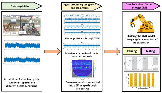
Figure 2.
Flow chart of proposed fault diagnosis method for gearbox.
4. Application of Fault Identification Scheme to DSG Test Rig Data
The raw vibration data was acquired from the DSG test rig shown in Figure 3. The DSG input shaft is driven by a 1.5 hp motor using a V-belt drive. A proximity sensor is used at the gearbox input shaft for measuring the speed. The vibration data is acquired by a uni-axial accelerometer sensor (PCB make) mounted on the casing of the gearbox with the help of a NI-DAQ system in the LabVIEW environment. The sampling rate for data acquisition was set at 20 kHz. Initially, the data was acquired for the healthy condition of the gearbox at three different input speeds of 972, 1205, and 1420 rpm.
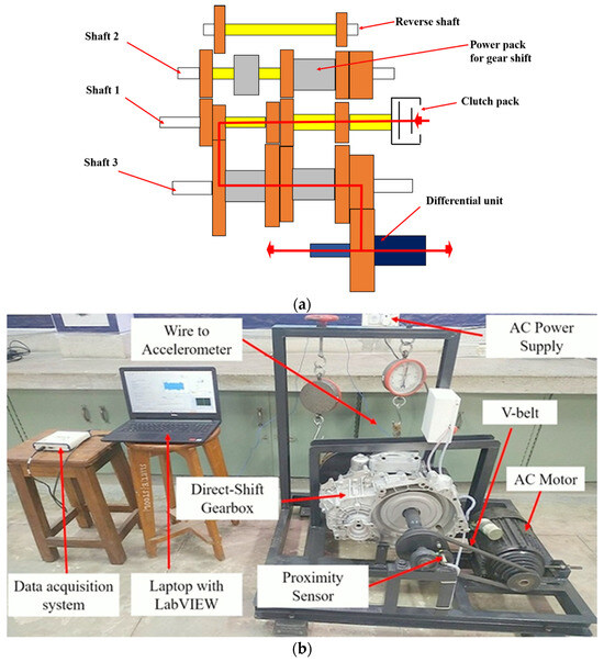
Figure 3.
Test rig (a) schematic view, and (b) pictorial view of an automatic transmission.
The raw vibration signal at 972 rpm under healthy conditions is shown in Figure 4a. It may include inherent defects (if any) present in the system. The acquired signal is processed by VMD, which decomposes it into different modes, as shown in Figure 4b. The statistical parameter, kurtosis, is used as a measurement index for identifying the consequences of impact in the signals. The kurtosis values obtained for six different modes of VMD are 2.95, 3.04, 3.00, 3.03, 2.92, and 3.02. It is observed that mode 2 has the highest value of kurtosis, i.e., 3.04. Thus, mode 2 is considered a prominent mode, which is further used to construct scalograms. The scalogram of the corresponding mode is shown in Figure 4c.

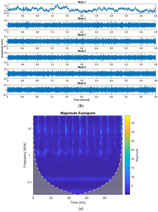
Figure 4.
(a) Raw signal; (b) decomposed signals; (c) scalogram of prominent mode (2) at 972 rpm under healthy conditions.
The other health condition that is used for analysis is tooth chipping. This defect is seeded in the DSG test rig to imitate the nature of chipping, which is induced by the localized stresses at the site of contact. In chipping, generally, some portion of the gear tooth is chipped off. The sensor mounted on the housing of the test rig acquires the raw vibration signal at 972 rpm, as presented in Figure 5a. The raw vibration signals under the chipping defect are further decomposed by the VMD, as shown in Figure 5b. The kurtosis value is computed for each mode, which is 2.96, 8.69, 2.97, 3.02, 2.91, and 3.03. As mode 2 has a maximum value of kurtosis, that means it represents the impact frequencies of the defects more effectively. Hence, to construct the scalogram, this particular mode is selected for further analysis. The corresponding scalogram is shown in Figure 5c.
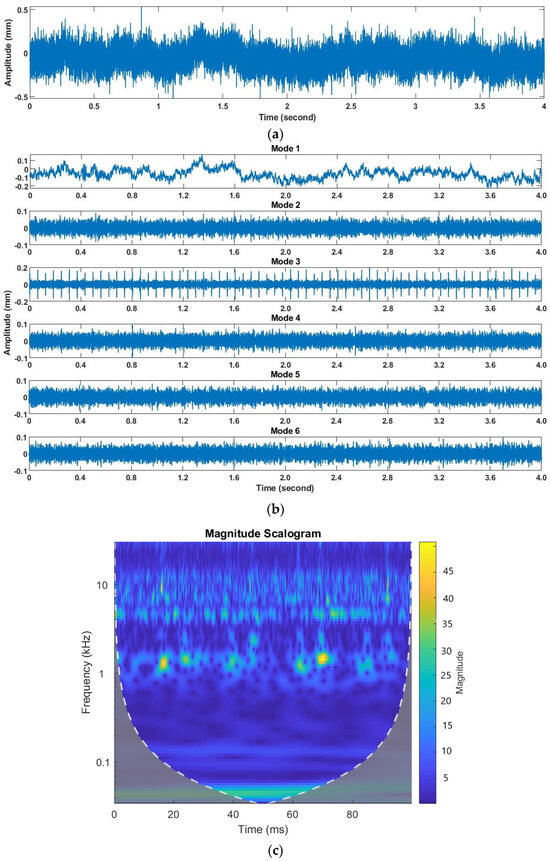
Figure 5.
(a) Raw signal; (b) decomposed signals; (c) scalogram at 972 rpm under tooth chipping condition.
Due to regular engagement and disengagement of the gear tooth, foreign particles, and burr, irregularities have been generated on the flank portion of the gear tooth. To seed this defect in the test rig, hammering or abrasive particles were used. The irregularities obtained at the flank portion of the gear tooth by the hammering or abrasive particles imitate the tooth-pitting defects. The test rig was operated at three different rpm, i.e., 972, 1205, and 1420. The raw vibration signal acquired at 972 rpm is shown in Figure 6a. VMD was used to process the raw vibration signal to decompose it into different modes, as shown in Figure 6b. The measurement index, i.e., kurtosis, was evaluated for each mode, whose values were 2.95, 3.02, 11.99, 3.04, 2.92, and 3.02. The kurtosis was maximum for mode 3, which means this particular mode contained high-impact frequencies. Thus, it was selected for constructing the scalogram for further analysis, as shown in Figure 6c.
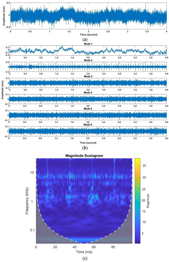
Figure 6.
(a) Raw signal; (b) decomposed signals; (c) scalogram at 972 rpm under tooth pitting condition.
5. Results and Discussion
Results of the CNN Model and Its Comparison with Other Classification Models
The methodology for identifying the different health conditions of the DSG test rig is explained in Section 4. Initially, the vibration data was acquired under different health conditions of the gearbox, and processed by the VMD technique. The parameters of VMD were obtained, as suggested in [27]. The scalogram was constructed for the prominent mode based on kurtosis. A total of 72 images were constructed with 24 images under each condition. Out of 72 images, 36 images (12 images under each health condition) were used for training the CNN model. The remaining 36 images were used as a testing data set. The size of each image was 227 × 227 × 3. The details of the training and testing data are provided in Table 1.

Table 1.
Detaining of Training and Testing data.
Table 2 briefly describes the CNN model’s design. The training accuracy of the developed CNN model is presented in Figure 7a,b as accuracy and loss, respectively. The model was then validated using test data. An attempt was also made to compare the proposed work to other classifiers, such as SVM and ELM. Table 3 shows that the CNN classifier performed better using the suggested method for all health conditions. The prediction results were also computed for various CNN sizes, which may be achieved by adding more convolution layers, as can be seen in Figure 8. The findings indicate that, when more than 5 convolution layers were utilized, the accuracy decreased but was recovered at a value of 8, implying that 5 convolution layers are sufficient for accurately forecasting the results.

Table 2.
Architect of CNN.
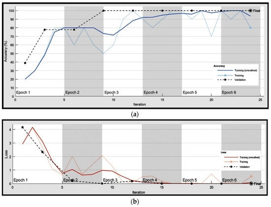
Figure 7.
(a) Training performance of CNN; (b) loss vs. iteration.

Table 3.
Comparison of CNN with SVM and ELM.
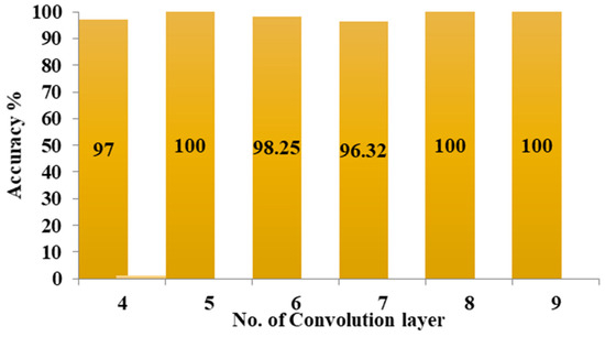
Figure 8.
Accuracy vs. no. of convolution layer.
The statistical analysis of the proposed method was carried out, in terms of accuracy, through one-way-ANOVA. The stated hypothesis of the one-way ANOVA are: H0 (null hypothesis). This suggests that there is no notable distinction in the accuracy of CNN compared to other algorithms. H1 (alternative hypothesis): there is a considerable distinction in accuracy between CNN and other methods.
To demonstrate the significance of the results obtained from the one-way ANOVA test, we compared the p-value with a specified value (α = 0.01 or α = 0.05).
- If the p-value is greater than 0.01, we accept the null hypothesis (H0) and reject the alternative hypothesis (H1), indicating that there is no significant difference between CNN and other methods of artwork.
- If the calculated p-value is below 0.05, then H1 is accepted and H0 is rejected, indicating a significant difference between CNN and other art methods.
Table 4 presents the findings of the one-way ANOVA test. The results indicate that the obtained p-value (0.0035) is lower than the significance level α (0.01), leading to the acceptance of the H1 hypothesis, indicating a significant difference in the results.

Table 4.
Statistical analysis of the proposed work.
6. Conclusions
In this work, vibration signal data was acquired from the DSG test rig, which was further processed by VMD. The prominent mode obtained through VMD, based on kurtosis, was used to construct a scalogram, and then an artificial intelligence-based CNN model was used to classify the different health conditions of the DSG. The following points have been concluded from the above study:
- (a)
- The signal-processing technique VMD, along with the statistical parameter kurtosis, plays a significant role in identifying the impact characteristics that are not observed in the raw vibration signal due to the transmission path.
- (b)
- The proposed fault identification scheme is capable of classifying the different health conditions with 100% accuracy.
- (c)
- The proposed fault identification scheme was compared with other classifiers in terms of classification accuracy. The results of the comparison show that the proposed fault identification scheme is at least 13.85% more reliable.
- (d)
- In the future, the authors will use techniques like synthetic data generation, noise addition, and signal transformation to create a more diverse and representative dataset. Also, the authors will attempt to tune the hyper-parameters of the CNN through optimization techniques.
Author Contributions
R.K. (Rishikesh Kumar): data curation and writing—original draft; P.K.: data curation and writing—original draft; G.V.: data curation, software, writing—original draft, and methodology; S.C.: data curation, software, writing—original draft, and methodology; R.Z.: writing—review and editing and supervision; S.K.: editing and methodology; R.K. (Rajesh Kumar): writing—review and editing and supervision; M.K.G.: writing—review and editing; N.S.R.: writing—review and editing. All authors have read and agreed to the published version of the manuscript.
Funding
This research received no external funding.
Data Availability Statement
Data can be made available at reasonable request.
Acknowledgments
The work is supported by the National Center of Science, Poland under Sheng2 project No. UMO-2021/40/Q/ST8/00024 “NonGauMech”—New methods of processing non-stationary signals (identification, segmentation, extraction, modelling) with non-Gaussian characteristics for the purpose of monitoring complex mechanical structures.
Conflicts of Interest
The authors declare no conflict of interest.
References
- Schmidt, S.; Zimroz, R.; Chaari, F.; Heyns, P.S.; Haddar, M. A simple condition monitoring method for gearboxes operating in impulsive environments. Sensors 2020, 20, 2115. [Google Scholar] [CrossRef]
- Schreiber, W.; Rudolph, F.; Becker, V. The new dual clutch gearbox from Volkswagen. ATZ Worldw. 2003, 105, 2–6. [Google Scholar] [CrossRef]
- Rathi, P.; Patil, P.A.J. Direct Shift Gear Transmission. In Proceedings of the 3rd International Conference on Ideas, Impact and Innovation in Mechanical Engineering (ICIIIME 2017), Pune, India, 1–2 June 2017; pp. 180–184. [Google Scholar]
- Huang, N.E.; Shen, Z.; Long, S.R.; Wu, M.C.; Shih, H.H.; Zheng, Q.; Yen, N.C.; Tung, C.C.; Liu, H.H. The empirical mode decomposition and the Hubert spectrum for nonlinear and non-stationary time series analysis. Proc. R. Soc. A Math. Phys. Eng. Sci. 1998, 454, 903–995. [Google Scholar] [CrossRef]
- Isham, M.F.; Leong, M.S.; Lim, M.H.; Ahmad, Z.A. Variational mode decomposition: Mode determination method for rotating machinery diagnosis. J. Vibroeng. 2018, 20, 2604–2621. [Google Scholar] [CrossRef]
- Singh, D.S.; Zhao, Q. Pseudo-fault signal assisted EMD for fault detection and isolation in rotating machines. Mech. Syst. Signal Process. 2016, 81, 202–218. [Google Scholar] [CrossRef]
- Chang, K.M. Ensemble empirical mode decomposition: A Noise-Assited. Biomed. Tech. 2010, 55, 193–201. [Google Scholar] [CrossRef]
- Yeh, J.R.; Shieh, J.S.; Huang, N.E. Complementary ensemble empirical mode decomposition: A novel noise enhanced data analysis method. Adv. Adapt. Data Anal. 2010, 2, 135–156. [Google Scholar] [CrossRef]
- Li, H.; Hu, Y.; Li, F.; Meng, G. Succinct and fast empirical mode decomposition. Mech. Syst. Signal Process. 2017, 85, 879–895. [Google Scholar] [CrossRef]
- Dragomiretskiy, K.; Zosso, D. Variational mode decomposition. IEEE Trans. Signal Process. 2014, 62, 531–544. [Google Scholar] [CrossRef]
- Zhao, Y.; Li, C.; Fu, W.; Liu, J.; Yu, T.; Chen, H. A modified variational mode decomposition method based on envelope nesting and multi-criteria evaluation. J. Sound Vib. 2020, 468, 115099. [Google Scholar] [CrossRef]
- Zhao, Y.X.; Li, Y.; Yang, B.J. Denoising of seismic data in desert environment based on a variational mode decomposition and a convolutional neural network. Geophys. J. Int. 2020, 221, 1211–1225. [Google Scholar] [CrossRef]
- O’Shea, K.; Nash, R. An Introduction to Convolutional Neural Networks. arXiv 2015, arXiv:1511.08458. [Google Scholar]
- Vashishtha, G.; Chauhan, S.; Kumar, S.; Kumar, R.; Zimroz, R.; Kumar, A. Intelligent fault diagnosis of worm gearbox based on adaptive CNN using amended gorilla troop optimization with quantum gate mutation strategy. Knowl.-Based Syst. 2023, 280, 110984. [Google Scholar] [CrossRef]
- Liu, C.; Cheng, G.; Chen, X.; Pang, Y. Planetary Gears Feature Extraction and Fault Diagnosis Method Based on VMD and CNN. Sensors 2018, 18, 1523. [Google Scholar] [CrossRef] [PubMed]
- Zhan, X.; Bai, H.; Yan, H.; Wang, R.; Guo, C.; Jia, X. Diesel Engine Fault Diagnosis Method Based on Optimized VMD and Improved CNN. Processes 2022, 10, 2162. [Google Scholar] [CrossRef]
- Xu, Z.; Li, C.; Yang, Y. Fault diagnosis of rolling bearing of wind turbines based on the Variational Mode Decomposition and Deep Convolutional Neural Networks. Appl. Soft Comput. 2020, 95, 106515. [Google Scholar] [CrossRef]
- Wu, Y.; Liu, L.; Qian, S. A small sample bearing fault diagnosis method based on variational mode decomposition, autocorrelation function, and convolutional neural network. Int. J. Adv. Manuf. Technol. 2023, 124, 3887–3898. [Google Scholar] [CrossRef]
- He, D.; Liu, C.; Jin, Z.; Ma, R.; Chen, Y.; Shan, S. Fault diagnosis of flywheel bearing based on parameter optimization variational mode decomposition energy entropy and deep learning. Energy 2022, 239, 122108. [Google Scholar] [CrossRef]
- Liu, Y.; Yang, G.; Li, M.; Yin, H. Variational mode decomposition denoising combined the detrended fluctuation analysis. Signal Process. 2016, 125, 349–364. [Google Scholar] [CrossRef]
- Lu, J.; Yue, J.; Zhu, L.; Li, G. Variational mode decomposition denoising combined with improved Bhattacharyya distance. Measurement 2020, 151, 107283. [Google Scholar] [CrossRef]
- Vashishtha, G.; Kumar, R. Centrifugal pump impeller defect identification by the improved adaptive variational mode decomposition through vibration signals. Eng. Res. Express 2021, 3, 035041. [Google Scholar] [CrossRef]
- Luo, J.; Wen, G.; Lei, Z.; Su, Y.; Chen, X. Weak signal enhancement for rolling bearing fault diagnosis based on adaptive optimized VMD and SR under strong noise background. Meas. Sci. Technol. 2023, 34, 064001. [Google Scholar] [CrossRef]
- Verstraete, D.; Ferrada, A.; Droguett, E.L.; Meruane, V.; Modarres, M. Deep learning enabled fault diagnosis using time-frequency image analysis of rolling element bearings. Shock Vib. 2017, 2017, 5067651. [Google Scholar] [CrossRef]
- Hoang, D.T.; Kang, H.J. Rolling element bearing fault diagnosis using convolutional neural network and vibration image. Cogn. Syst. Res. 2019, 53, 42–50. [Google Scholar] [CrossRef]
- Vashishtha, G.; Kumar, R. An amended grey wolf optimization with mutation strategy to diagnose bucket defects in Pelton wheel. Measurement 2022, 187, 110272. [Google Scholar] [CrossRef]
- Vashishtha, G.; Kumar, R. An effective health indicator for the Pelton wheel using a Levy flight mutated genetic algorithm. Meas. Sci. Technol. 2021, 32, 094003. [Google Scholar] [CrossRef]
Disclaimer/Publisher’s Note: The statements, opinions and data contained in all publications are solely those of the individual author(s) and contributor(s) and not of MDPI and/or the editor(s). MDPI and/or the editor(s) disclaim responsibility for any injury to people or property resulting from any ideas, methods, instructions or products referred to in the content. |
© 2024 by the authors. Licensee MDPI, Basel, Switzerland. This article is an open access article distributed under the terms and conditions of the Creative Commons Attribution (CC BY) license (https://creativecommons.org/licenses/by/4.0/).