Review

A Review on the Applications of Dual Quaternions

by
João Gutemberg Farias
1,*,
Edson De Pieri
2 and
Daniel Martins
3
1
Academic Unit of Cabo de Santo Agostinho, Federal Rural University of Pernambuco, Cabo de Santo Agostinho 54518-430, PE, Brazil
2
Department of Automation and Systems, Federal University of Santa Catarina, Florianópolis 88040-900, SC, Brazil
3
Department of Mechanical Engineering, Federal University of Santa Catarina, Florianópolis 88040-900, SC, Brazil
*
Author to whom correspondence should be addressed.
Machines 2024, 12(6), 402; https://doi.org/10.3390/machines12060402
Submission received: 20 March 2024 / Revised: 1 May 2024 / Accepted: 7 May 2024 / Published: 12 June 2024
(This article belongs to the Special Issue Control and Mechanical System Engineering)

Abstract

:
This work explores dual quaternions and their applications. First, a theoretical construction begins at dual numbers, extends to dual vectors, and culminates in dual quaternions. The physical foundations behind the developed theory lie in two important fundamentals: Chasles’ Theorem and the Transference Principle. The former addresses how to represent rigid-body motion whereas the latter provides a method for operating on it. This combination presents dual quaternions as a framework for modeling rigid mechanical systems, both kinematically and kinetically, in a compact, elegant and performant way. Next, a review on the applications of dual quaternions is carried out, providing a general overview of all applications. Important subjects are further detailed, these being the kinematics and dynamics of rigid bodies and mechanisms (both serial and parallel), control and motion interpolation. Discussions regarding dual quaternions and their applications are undertaken, highlighting open questions and research gaps. The advantages and disadvantages of using dual quaternions are summarized. Lastly, conclusions and future directions of research are presented.

1. Introduction

The general displacement of a rigid body can be represented in terms of points or in terms of lines. Although the most commonly adopted method to represent the displacement is point-based, which is the homogeneous matrix, it is not the only possible representation. In many cases, it is not the best [1]. On the other hand, arguably, lines are more fundamental than points since they can be used to represent rotations and forces. Also, their linear combination, screws, can represent twists and wrenches [2].
When investigating line-based methods, dual quaternions stand out as a powerful, concise and elegant tool to represent and operate on rigid-body movement, and, furthermore, they relate strongly to Screw Theory. Representing and operating on rigid motion allow using this tool in a great range of applications. Additionally, Screw Theory provides a paradigm shift in modeling problems that may result into new insights and simpler models.
However, dual quaternions require a theoretical background unfamiliar to most engineers, comprising concepts such as dual numbers, line vectors, dual vectors, quaternions, line transformations and Screw Theory [3]. And, as much as it provides advantages over other formulations with its creation being not recent [4], the use of this tool, although increasing, is below its potential.
Therefore, the authors herein aim to present dual quaternions with a solid background coming from dual numbers and showing the duality of vectors and lines, as well as its strong relation to Screw Theory. We introduce dual quaternions as a tool with many applications, conveying a systematic review of its applications dating from 1964 to 2024. We detail fundamental applications as kinematics, dynamics and control and motion interpolation, which, combined, place dual quaternions as a framework for working with mechanism and robotics. Lastly, dual quaternions are useful not only to researchers familiar with the tool and already applying it, but also to researchers looking enter the field. We hope to facilitate this not only by providing a solid foundation, but also by discussing more in depth its applications and providing open questions and research gaps.
To deal with the above considerations, this work is divided into three parts. The first part builds the theoretical background. The second part consists of a review of the applications using dual quaternions. We not only mention, but also to show how dual quaternions can be de facto used in some key applications. The third part discusses the applications, presents venues for new research and has the closing sections.
Chasles’ Theorem and the Transference Principle are the physical foundations behind the first part. Chasles’ Theorem exposes the close relation between twists (also lines and screws) and rigid-body motion. The Transference Principle provides us with a method to transition from a formulation to operate on vectors into one to operate on lines and twists using dual quantities.
Going through the theoretical background in the Section 2 of this work, we formalize the Transference Principle and present dual numbers and the concept of dual functions and dual angles. In Section 3, we introduce Chasles’ Theorem and present dual vectors as a means to represent lines, screws and twists. Finally, Section 4 defines dual quaternions and how to use them to operate on dual vectors.
After the theoretical background, the next part of this work, Section 5, reviews the applications using dual quaternions. We present a general overview of the applications, then we further explore important subjects; these subjects being rigid-body motion, serial mechanisms, parallel mechanisms, control and rigid-body motion interpolation.
The third part starts with Section 6 by adding relevant discussions over dual quaternions and their applications, showing unanswered questions and research gaps. We finalize the section by presenting a compilation of the advantages and disadvantages of dual quaternions mentioned throughout this review of its applications. The last two sections present the conclusions (Section 7) and future directions of research (Section 8).
This paper is the first review article focused on dual quaternions applications. The novel contributions coming from this work are the systematic review of applications dating from 1964 to 2024 and ranging from the first kinematics articles to new and unexpected applications like Origami Systems and Neural Networks. Additionally, there are discussions over important topics (related to dual quaternions and their applications) with the introduction of open questions and research gaps that can be exploited by both novice and experienced researchers on the field. Lastly, a dedicated section on the advantages and disadvantages of using dual quaternions is collated from the reviewed articles. These combined contributions reduce the initial barrier necessary for the accomplishment of any dual quaternion-related work.
Notation: We will represent scalar variables in lowercase, angles with Greek letters, vector quantities with bold letters and quaternions with q. Dual quantities will have a hat over them, in which their primary part will have the same notation as the quantity they represent and the dual part will have an underscore “o”, like in v ^ = v + v o . A real unitary entity will have an underbar, like in s ̲ . A dual unitary entity will also have an underbar but its parts will have an underbar for the primary part and an “underharpoon” for the dual part, as in q ^ ̲ = q ̲ + q o .

2. Dual Numbers

In this section we introduce the Transference Principle, which is one of the cornerstones of the theory developed throughout the first part of this work. After that, dual numbers are defined, followed by dealing with functions of dual numbers and their trigonometry.

2.1. Transference Principle

The Transference Principle was first stated by Kotelnikov [5] and soon after by Dimentberg [6]. Still, there have been equivalent statements from others like Rooney [7] and Martinez [8] (see this work for more on the history and proof of the principle). Although the statements are different, the core idea remains the same. We have made a version of the statement using the ideas in the articles cited above but making amends when necessary to due to the limitations pointed out by [9].
On one side, we have the intersecting lines, vectors, spherical geometry and rotation group ( S O ( 3 ) ). On the other side we have the skew lines, screws, spatial geometry and Euclidean group ( S E ( 3 ) ). The Transference Principle states that if we take one algebraic equation involving the components of the first side and apply a dualization process, we obtain a valid algebraic equation involving the components of the second side. The dualization process consists of replacing every real variable x for a corresponding dual variable x ^ = x + ε x o . (For a proof of the Transference Principle, look at [8,9,10]. According to the proofs in the cited works, the above statement falls short of the principle capabilities, it can comprehend also differential calculus and calculations in Lie groups.)
The Transference Principle can have a pure geometrical interpretation, but its practical implications are tremendous. One significant consequence of the principle of transference is that every algebraic equation involving only rotations becomes, after a dualization, a valid algebraic equation involving rotation and translation. Another equally important consequence is that operators of rotation, like orthogonal matrices and quaternions, become, after a dualization, operators of both rotation and translation, like dual orthogonal matrices and dual quaternions.

2.2. Definition of Dual Numbers

Dual numbers came to light in the same work where Clifford introduced dual quaternions [4], but what started as a simple algebraic tool soon had its potential realized independently by Kotelnikov [5] and Study [11] in the field of kinematics.
A dual number is defined around the dual operator ε , which has the property of ε 2 = 0 but ε 0 . It takes the form
a ^ = a + ε a o ,
where a , a o in R . We say that a ^ is a dual number (or a ^ D ), with a being its primary part and a o being its dual part. We can otherwise denote the primary part as R { a ^ } and the dual part as D { a ^ } . The dual operator commutes with real numbers, that is 1 ε = ε 1 = ε , also 0 ε = ε 0 = 0 . Taking a ^ = a + ε a o and b ^ = b + ε b o , dual numbers have the following algebraic properties [12]:
  • Equality: a ^ = b ^ iff a = b and a o = b o .
  • Addition: a ^ + b ^ = ( a + ε a o ) + ( b + ε b o ) = ( a + b ) + ε ( a o + b o ) .
  • Multiplication: a ^ b ^ = ( a + ε a o ) ( b + ε b o ) = a b + ε ( a b o + b a o ) .
  • Division: the division a ^ / b ^ is possible and unambiguous if b 0 and takes the form
    a ^ b ^ = a + ε a o b + ε b o = a b + ε a o b a b o b 2 , ( b 0 ) .

2.3. Functions of Dual Numbers

Let f be a smooth real number function, or f : R R , and we can extend/dualize its behavior to a dual number function f ^ : D D by [9]:
f ^ ( x ^ ) = f ^ ( x + ε x o ) = f ( x ) + ε x o f x ( x ) .
As these dual-valued functions are extensions of real-valued ones, we are going to drop the hat over the function and denote both functions the same way, so it should be straightforward to distinguish them by context.
For example, consider the square root function. Its extension for a function of dual numbers can be obtained as follows:
x ^ = x + ε x o 1 2 x .

2.4. Trigonometry

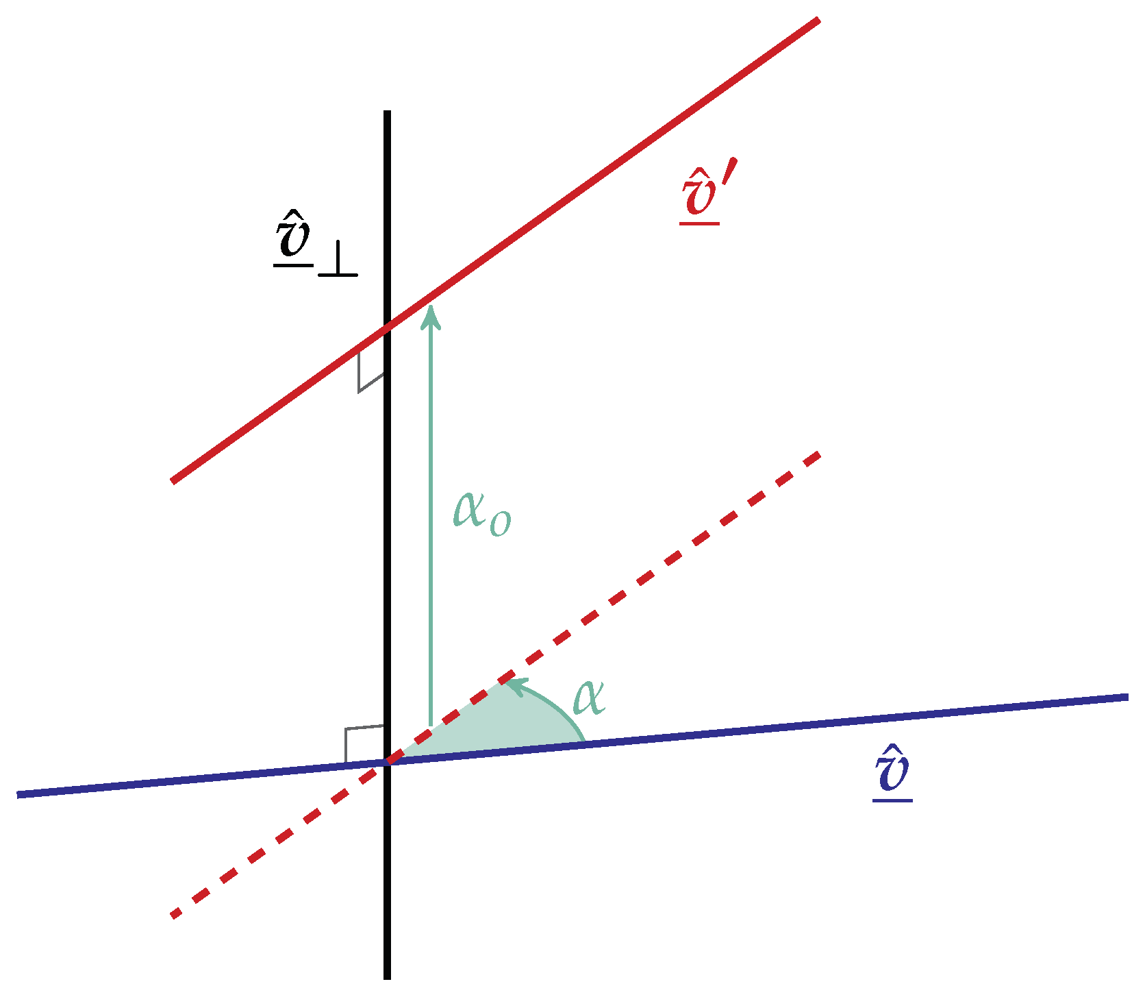
As the real angle expresses the relation between two vectors (Figure 1a), the dual angle expresses the relation between two straight lines in space. Take two lines and the common normal line between the two: if we rotate the first line around the common normal, we can make it become parallel to the second, and then we translate the first line toward the common normal to make the two lines coincide.
To relate two lines, we need a rotation and a translation. The dual angle is a quantity that can do both, where the primary part expresses the rotation and is the angle between the two lines (around the common normal) and the dual part expresses the translation and is the distance (along the common normal) between the two lines (Figure 1b).
According to Equation (3), we can compute the sine and cosine of a dual angle ( α ^ = α + ε α o ) by:
cos ( α ^ ) = cos ( α ) ε α o sin ( α ) ,
sin ( α ^ ) = sin ( α ) + ε α o cos ( α ) .
Using the Equations (5) and (6), all trigonometric identities valid for ordinary angles remain valid for dual angles [13].

3. Dual Vectors

We begin this section by briefly stating Chasles’ Theorem (the other cornerstone of the theory developed) before delving into Dual Vectors and their connection to lines and screws.

3.1. Chasles’ Theorem

Chasles’ Theorem statement:
Any given displacement of a rigid body can be effected by a rotation about an axis combined with a translation parallel to that axis.
There are many ways to represent the displacement of a rigid body, with displacement meaning a combination of rotation and translation. But Chasles’ Theorem stands apart from the other representations, as in the words of Sir Robert Ball [14], it is “the reduction of the displacement to its simplest form, in which no arbitrary element is involved”. Chasles’ statement makes us realize that something so simple and geometrically pure as a line is closely related to how a rigid body moves.

3.2. Definition of Dual Vectors

Dual vectors are vectors whose components are dual numbers instead of real numbers; they can also be thought of as a pair of vectors, one real and another dual. That is
v ^ = v x + ε v o x v y + ε v o y v z + ε v o z = v + ε v o ,
where v ^ is a dual vector, v = ( v x , v y , v z ) and v o = ( v o x , v o y , v o z ) .

3.3. Norm of a Dual Vector

The 2-norm of a general dual vector can be computed as a generalization of the function
| | v | | = f ( v ) = v · v
to the domain of the dual vectors. The operator · represents a vector dot product.
The same generalization/dualization process of Equation (3) can be applied to the domain of real/dual vectors, resulting in [8]
f ( v ^ ) = f ( v + ε v o ) = f ( v ) + ε v o · ( f ) ,
where f = f x , f y , f z .
So, using Equation (9),
| | v ^ | | = f ( v + ε v o ) = | | v | | + ε v o · v | | v | | .
Notice that | | v ^ | | is not well defined when | | v | | = 0 and the norm of a dual vector is a dual number. The same result can be obtained using Equation (4).

3.4. Representation of Lines by Dual Vectors

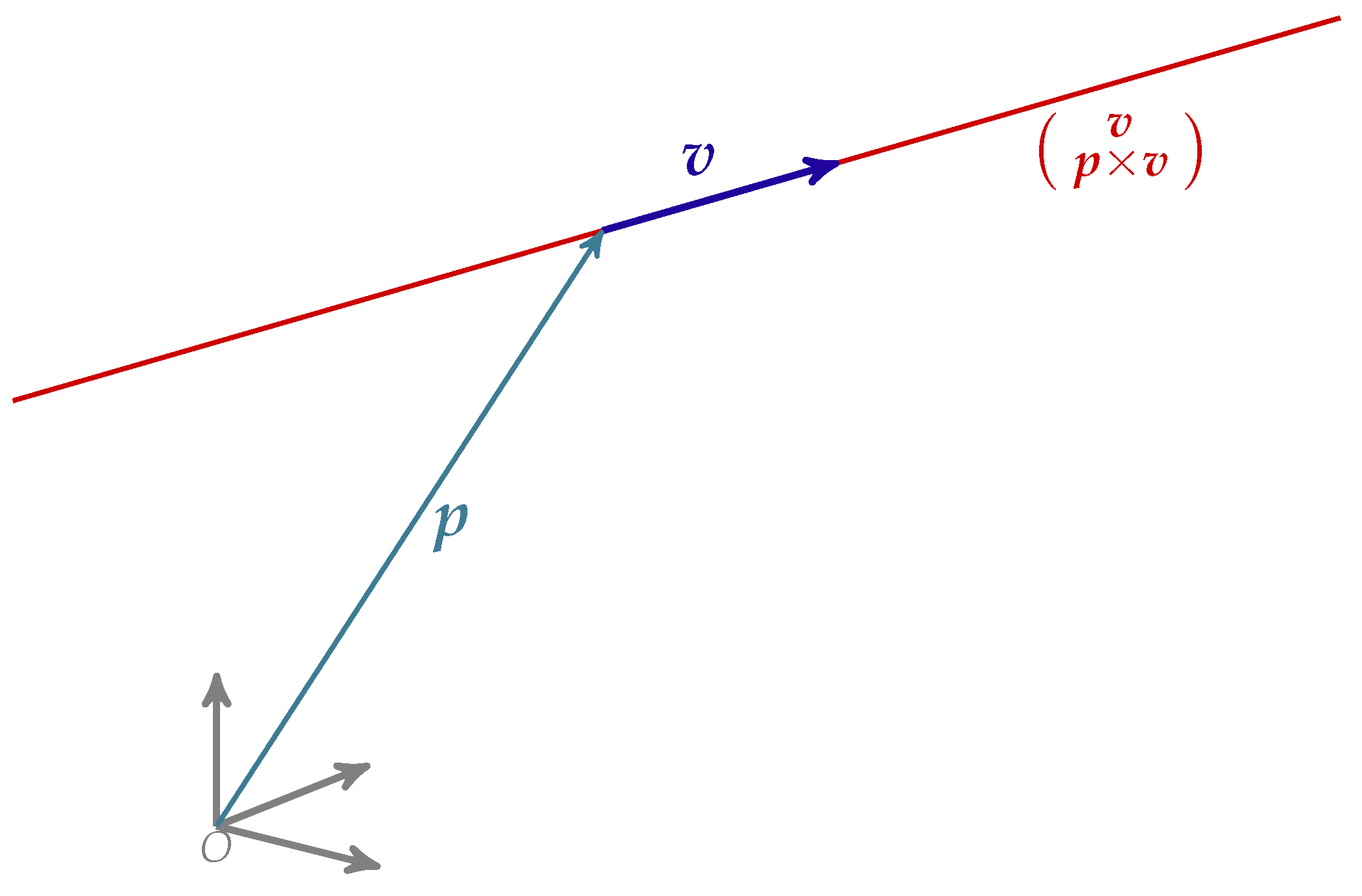
Dual vectors can represent straight lines (line vectors) like Plücker coordinates but with a complete set of algebraic tools. We use v to be the direction of the line and v o = p × v to be the moment of the line (Figure 2).
In fact, we can obtain lines from unit vectors using the generalization/dualization process of Equation (9). If we dualize the restriction for a unitary vector ( v · v = 1 ), we obtain, by applying Equation (9) to f ( v ) = v · v = 1
f ( v ^ ) = v · v + ε ( v o · 2 v ) = 1 + ε 0 ,
which can be separated into two conditions
v · v = 1 and v · v o = 0 .
The conditions of Equation (12) are the same that Plücker coordinates must adhere to represent a line. Actually, those are stronger conditions, and a weaker one is just v · v o = 0 ; as Plücker coordinates are homogeneous, they still represent the same line no matter the norm of v . As [8] stated, “the image of an arbitrary unit vector under the dual mapping is the set of lines whose direction is given by the original vector”. Observe that v ^ and v ^ represent the same line, and in fact each dual vector satisfying Equation (12) represents not only a line but also an oriented line with the orientation given by the primary component. Although it is important to remember that they are oriented lines, most of the time it is enough to treat them generically as lines.
With a dual vector representing a line, v o · v = 0 , and the norm from Equation (10) reduces to | | v ^ | | = | | v | | . That is, the dual norm is equal to the real norm.
The dot product and cross product of lines are similar to their counterpart for vectors [12]:
v ^ 1 · v ^ 2 = | | v ^ 1 | | | | v ^ 2 | | cos ( α ^ ) dot product of lines ,
v ^ 1 × v ^ 2 = | | v ^ 1 | | | | v ^ 2 | | sin ( α ^ ) v ^ ̲ cross product of lines .
where v ^ ̲ is a line intersecting and orthogonal to both v ^ 1 and v ^ 2 .

3.5. Representation of Screws and Twists by Dual Vectors

A twist is comprised by a rotation around an axis (a line), w ^ = w + ε ( p × w ) , with intensity | | w | | , and a translation toward the same axis, ν ^ = ε ν , with intensity | | ν | | .
The twist ( S ^ ) is then the sum of rotation and translation contributions. But as w and ν have the same direction, they are thought to be related by a pitch, much like the pitch of a real screw. So, we can write ν = h w , where h is the so-called pitch. This leads us to
S ^ = w + ε ( p × w + h w ) .
The screw is a pure geometrical entity created by Sir Ball, comprising a line associated with a pitch. It is the geometric entity carrying the twist, and the twist is nothing but a screw with physical meaning and the dimension of angular velocity in the primary part and linear velocity in the dual part, obtained by multiplying a screw by an angular velocity.
To obtain a screw from a twist, we need to separate it from its real norm (the norm of the rotation), i.e., S ^ = | | w | | s ^ . The term s ^ has the information of the axis and also the information of the pitch, so it is then the aforementioned screw. Expanding this,
s ^ = w ̲ + ε ( p × w ̲ + h w ̲ ) .
The representation of a screw is basically the same as a line, where the real part still has to be unitary; the difference is that the dual part needs not be orthogonal to the real part. The screw has five degrees of freedom, one more than the line due to the pitch. The twist has six, the five of the screw plus the rotation magnitude, thus encompassing the six degrees of freedom of a free rigid body.
Another way to think of a twist, besides as an intensity of rotation applied to a screw, is as a dual rotation applied to an axis. Let s ^ ̲ be the axis of the twist, then
S ^ = ( w + ε ν ) s ^ ̲ = ( w + ε h w ) s ^ ̲ .
Equation (17) gives us a clear idea of how dual numbers and twists go well together. A dual number multiplied by a dual vector line yields a twist in which the line gives the axis, the magnitude of rotation by the primary part of the dual number and the magnitude of translation by its dual part. The same goes for the screw, using dual numbers we can algebraically separate the pitch and the axis as s ^ = ( 1 + ε h ) s ^ ̲ .
This approach is very useful, as we already have the algebra of dual vectors representing lines (mainly the dot product of lines, Equation (13), and the cross product of lines, Equation (14)), so when we separate a screw or twist as a norm (dual number) and an axis (straight line), we can operate on them individually by treating them separately. So, for example, if we were to take the dot product of two twists S ^ 1 = | | S ^ 1 | | s 1 ^ and S ^ 2 = | | S ^ 2 | | s 2 ^ , the result can be computed simply by
S ^ 1 · S ^ 2 = | | S ^ 1 | | s 1 ^ · | | S ^ 2 | | s 2 ^ = | | S ^ 1 | | | | S ^ 2 | | ( s ^ 1 · s ^ 2 )
S ^ 1 · S ^ 2 = | | S ^ 1 | | | | S ^ 2 | | cos ( α ^ ) .

4. Dual Quaternions

We end the first part of this work, the theoretical background, by defining Dual Quaternions and showing how they operate on lines by means of the Left Operator (Section 4.3.1) and the General Twist Operator (Section 4.3.2).

4.1. Definition of a Dual Quaternion

Dual quaternions are quaternions (for a reminder of quaternions’ properties, see [2]; for a more comprehensive study, we recommend [15]) whose components are dual numbers instead of real numbers. They can also be thought as a dual scalar and a dual vector or as a pair of quaternions, one real and another dual. That is
q ^ = q ^ 0 + q ^ 1 i + q ^ 2 j + q ^ 3 k = q ^ 0 + q ^ = q + ε q o ,
where q ^ is the dual quaternion, q ^ = q ^ 1 i + q ^ 2 j + q ^ 3 k is a dual vector, q and q o are quaternions. Dual vectors can be considered dual quaternions whose dual scalar is zero. This notion will be used throughout the rest of this work. Also, mind the writing difference between the dual scalar q ^ 0 and the quaternion q o .
The operations on dual quaternions are straightforward: sum and subtraction are trivial and multiplication follows the multiplication of individual quaternions as
q ^ a q ^ b = ( q a + ε q a o ) ( q b + ε q b o ) = q a q b + ε ( q a q b o + q a o q b ) .

4.2. Norm of a Dual Quaternion

Analogously to the norm of a quaternion, the norm of a dual quaternion can be computed by
| | q ^ | | = q ^ q ^ * = q ^ * q ^ = q ^ 0 2 + q ^ · q ^ ,
notice that
q ^ q ^ * = q q * + ε ( q q o * + q o q * ) ,
q ^ * q ^ = q * q + ε ( q * q o + q o * q )
and we know that the real part q q * = q * q is a real number. But, it turns out that the dual part
q q o * + q o q * = q * q o + q o * q = 2 ( q 0 q o 0 + q · q 0 )
is also a real number, where q ^ * = q ^ 0 q ^ = q * + ε q o * is the conjugate of q ^ . This makes the identity q ^ q ^ * = q ^ * q ^ true and results in a dual number. Also, given two quaternions q and r, we can define a dot operation on quaternions by
q · r = q 0 r 0 + q · r .
With q ^ q ^ * being a dual number we have to take the square root considering a function of a dual number, which, remembering from Equation (3),
f ( x + ε x o ) = f ( x ) + ε x o f ( x ) .
So the resulting square root is
| | q ^ | | = q ^ q ^ * = q q * + ε q q o * + q o q * 2 q q * | | q ^ | | = q ^ q ^ * = | | q | | + ε q q o * + q o q * 2 | | q | | ,
notice that the norm is only well defined when | | q | | > 0 . Using Equation (25) and the dot product of quaternions defined at Equation (26), we can rewrite the equation as
| | q ^ | | = q ^ q ^ * = | | q | | + ε q · q o | | q | | .
It is possible to decompose a dual quaternion in its norm multiplied by a unit dual quaternion as
q ^ = | | q ^ | | ( | | q ^ | | 1 q ^ ) = | | q ^ | | q ^ ̲ ,
where q ^ ̲ is the unit dual quaternion associated with the dual quaternion q ^ .
We denote a unit dual quaternion by q ^ ̲ = q ̲ + ε q o , where the “underharpoon” in q o means that it satisfies q ̲ q o * + q o q ̲ * = 0 (or, q ̲ · q o = q 0 q o 0 + q · q o = 0 ), which leads to q ^ ̲ q ^ ̲ * = q ^ ̲ * q ^ ̲ = 1 + ε 0 . Unit dual quaternions are very important because they are the ones that operate on lines, where the unitariness comes in handy as they do not scale the lines or transform them into screws or twists.

4.3. Dual Quaternion Operations

Like quaternions, dual quaternions are not commutative. This results in different effects when applied from the right or from the left. The operators in dual quaternions take the form of a left operator (Section 4.3.1) and a left and right (often called sandwich) operator (Section 4.3.2).

4.3.1. Left Operator

As the left operator in quaternions is used to rotate vectors around an orthogonal vector, using the Transference Principle we can deduce that by a dualization, the same operator as a dual quaternion can be used to rotate and translate a line. To do that, we use a unit dual quaternion to left multiply a dual vector representing a line (unit dual vector). The dual quaternion axis (given by its vector part) and the axis of the line we are trying to operate on must be orthogonal and intersecting. The construction of the operator q ^ ̲ follows the quaternionic one by a dualization
q ^ ̲ = cos ( α ^ ) + sin ( α ^ ) v ^ ̲ ,
which accounts for a dual rotation α ^ around the axis v ^ ̲ , i.e., a rotation α around the axis and a translation α o along the axis, with the condition that v ^ ̲ is perpendicular to the line we are operating on and they intersect. Figure 3 illustrates the dual rotation given by the equation
v ^ ̲ = q ^ ̲ v ^ ̲ .
Note that dual vectors are treated as dual quaternions with only the vector part (scalar part is zero). That way, the above product makes sense.

4.3.2. General Twist Operator

The general twist operator in the dual quaternions, analogously to the case of the general rotation operator in quaternions, comes without the limitations of the left operator. Using this new operator, we can perform a twist in an arbitrary line.
We use the half dual angle and a line vector as a unit dual vector to construct the operator axis. The construction is made by
q ^ ̲ = cos α ^ 2 + sin α ^ 2 v ^ ̲ r ,
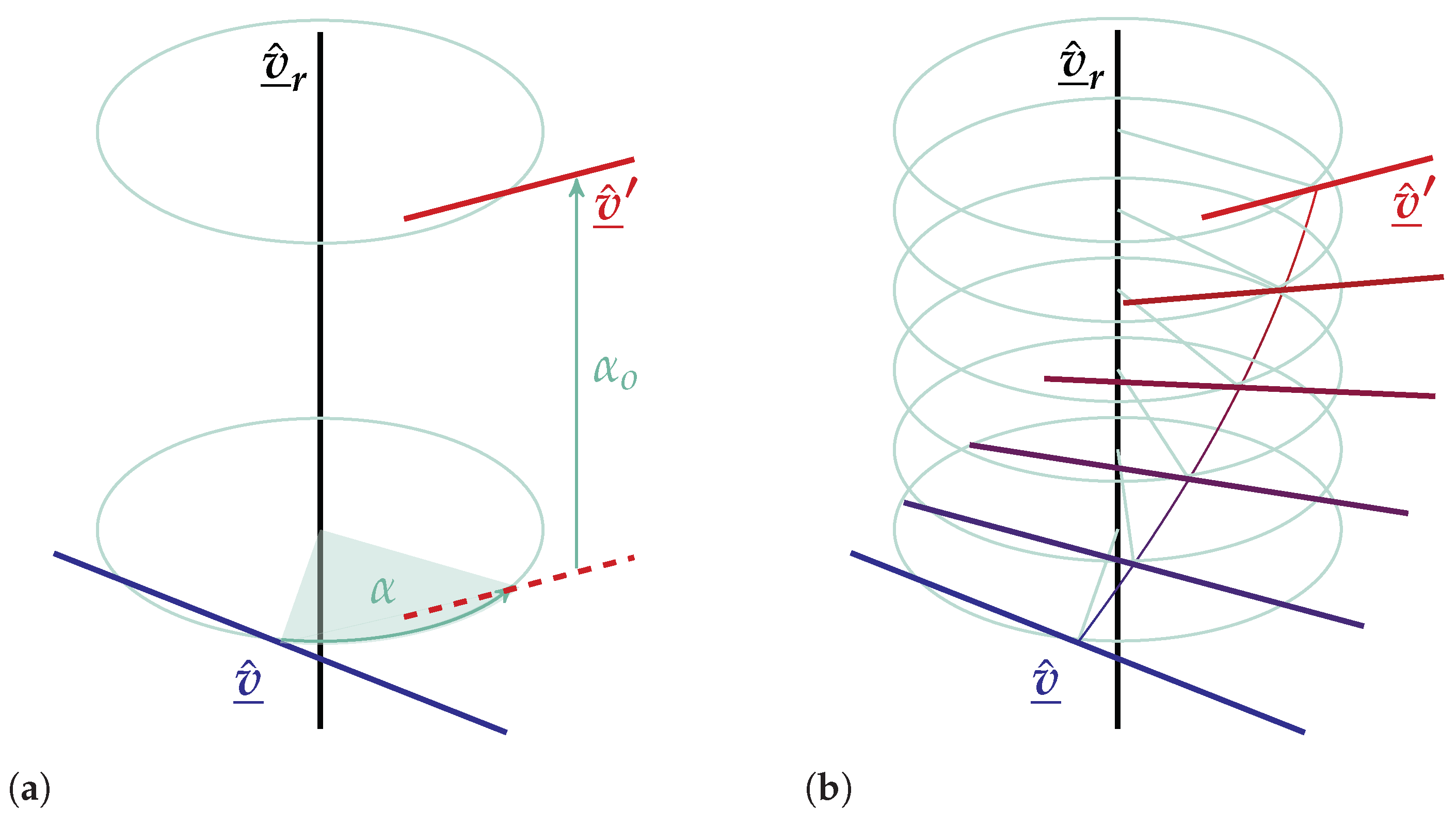
where α ^ = α + ε α o is the dual angle consisting of a rotation α and a translation α o , and v ^ ̲ r is the unit dual vector containing the axis of the operation. The operation aims to perform a twist given by a rotation α around the axis v ^ ̲ r and a translation α o along the same axis.
Once we have constructed q ^ ̲ , the operation comprises multiplying a dual vector on the left by q ^ ̲ and on the right by q ^ ̲ * ; because of this, it is sometimes referred to as a “sandwich operation”. The operation is computed by
v ^ ̲ = q ^ ̲ v ^ ̲ q ^ ̲ * ,
where v ^ ̲ is the operated dual vector and v ^ ̲ is the resulting dual vector. Figure 4 illustrates the dual rotation.
This operation is shown to be equivalent to the dual Euler–Rodrigues formula [16] for performing rigid-body motion (the general rotation operation using quaternions is likewise shown to be equivalent to the Euler–Rodrigues formula [17] for rotating vectors).

4.3.3. The “qt” Twist Operator

The qt twist operator is a very useful form of the general twist operator that allows us to rotate a line by a quaternion and translate it by a vector without the formalism of the twist. The operator construction is as simple as
q ^ ̲ = q ̲ + ε t q ̲ 2 ,
where q ̲ is a quaternion constructed using the quaternionic general rotation operation, which handles the rotation of the operated line, and t is a vector containing the desired translation.
The operation performs a rotation of the line done by the quaternion q ̲ . This corresponds to a rotation about a line going through the origin and having the direction of q ̲ , i.e., the operated line performs a circular motion about the origin. After the rotational motion, the line translates by t . Figure 5 illustrates the resulting motion of a qt twist operator. In the image v ^ ̲ r is the operating line ( v ^ r is the line made by the direction v r on quaternion q ̲ and passing through the origin).
The qt operation shares a special bond with the general twist operation, as it is possible to build one using the other, so they are two ways of representing the same operation. Also, as is evident from the qt formulation but hard to see from the other twist operator, we can compute the pure translation associated with a general twist operator q ^ ̲ = q ̲ + ε q o by
t = 2 q o q ̲ * .
Note that the vector t does not consider the translation due to the rotation around the origin of the reference frame, as shown in Figure 5. But, if the operated line crosses the origin, then t encompasses all the translation carried out by the operation.
Another way to apply this operator is to use it as q ^ ̲ = q ̲ + ε q ̲ t s 2 . The translation is applied before the rotation [18].

5. Dual Quaternions Applications

The second part of this work deals with the review of the applications of dual quaternions. We start by providing a chronological general overview of the applications, dating from 1964 to 2024. When focusing in one application, we follow its development in time before going to the next. After the general overview, key applications of dual quaternions are detailed, these being the kinematics and dynamics of rigid bodies and mechanisms, control and motion interpolation.

5.1. General Overview

The first obvious application of dual quaternions was to describe the kinematics of rigid bodies and mechanisms. Yang and Freudenstein [19] were among the first to apply dual quaternions, in 1964, to compute the kinematics of a parallel mechanism; in that case, the mechanism was a spatial four-link mechanism with one turning pair and three turn-slides; Yang also applied to a serial mechanism soon after [20].
More works on kinematics using dual quaternions were published [1,2,3,12,21], but now as a general technique for kinematics (kinematics of rigid bodies, direct kinematics of serial mechanisms and differential kinematics) and not as an analysis of a particular mechanism as Yang and Freudenstein did. Gupta [22,23] developed the method of Successive Screw Displacements. Özgür and Mezouar [24] follow the Screw Theory approach and use Successive Screw Displacements to propose a general framework for the kinematic modeling of serial robots.
To this day, kinematics is still a major research subject in dual quaternions. More specific works include the forward kinematics of parallel mechanisms [25,26,27,28,29] and the inverse kinematics of serial mechanisms using dual quaternions and screw theory, mainly based on Paden–Kahan sub-problems and extensions to the sub-problems [30,31,32,33], and overconstrained spatial mechanisms [34]. Recent works are experimenting with hyper-dual quaternions [35,36,37,38], which can compute both kinematics and differential kinematics at the same entity by exploiting the property of dual numbers called Automatic Differentiation. Figure 6 shows a timeline of the kinematics-related articles reported in this work.
Despite Yang [39] exploring the subject in his early works, the field of dynamics received little attention. Later, an important contribution was made by [43] introducing the dual inertia operator, creating a formulation that “unifies” twists and wrenches. Although this formulation is not widely used, it is gaining popularity. Nevertheless, interesting works are being carried out focusing on dynamics, like [52] describing a framework to derive the dynamics of a satellite and [53] completing a performance study on a Recursive Newton–Euler Inverse Dynamics Algorithm using dual quaternions. Silva [54] develops two approaches to the dynamics of mobile manipulators using dual quaternions: one approach uses Recursive Newton–Euler and the other uses Gauss’s Principle of Least Constraint. Recently, ref. [55] introduced for the first time Lagrange’s dynamic equations in dual quaternion form.
Non-kinematics-related works started modestly in the 1990s. Walker et al. [56] applied dual quaternions to estimate the pose of an object using visual data and [44] used them to interpolate rigid-body motion. Both became more active areas of research recently, the first (visual data processing and cloud points registration) being followed by [57,58,59,60] and the second (interpolation of rigid-body motion) followed by [61,62,63,64] (alternatively to motion interpolation, ref. [65] uses differential geometry and dual curvature theory). Relative to the topic of motion interpolation, ref. [66] developed, based on dual quaternions, a novel kinematic measure of mean (average) and variance of spacial displacements. Path planning of robots and manipulators are being accomplished through motion interpolation where global poses are defined previously and the path connecting theses poses is derived continuously through the dual quaternion’s Screw Linear Interpolation (Screw Linear Interpolation, or sclerp, will be discussed in more detail in Section 5.6) [67,68,69]. Another important work, at the end of the decade, was the hand–eye calibration in [70], which, together with robot–world and robot–robot calibration, is still an active research area in dual quaternions [71,72,73,74,75].
In the 2000s, ref. [76] applied dual quaternions to the problem of kinematic synthesis and [77] rewrote the equations for strapdown inertial navigation systems using dual quaternions and Screw Theory. Later in the same decade, the works of control using dual quaternions appeared as kinematic control [78]. After that, the number of works in this area increased rapidly, featuring dual quaternion PID [79], kinematic control [24,80,81], feedback linearization [82,83,84,85,86], model predictive control [69,87,88], adaptive control [47,89] (ref. [90] used adaptive control to perform kinematic-model-free control, in which no previous knowledge of the kinematic model or even joint variables is required to move the end-effector to the desired pose), sliding modes [91,92], H [46] and backstepping [93,94]. Figure 7 shows a timeline of the control-related articles reported in this work.
From 2010 to 2021, the number of articles applying dual quaternions increased rapidly. Works dealing with proximity operations on spacecrafts, like rendezvous and docking, using dual quaternions to model the relative pose between chaser and target spacecrafts ranges from different areas like visual data processing [57] and Kalman filter [101] for estimating the relative pose and controllers to guarantee a smooth approximation of the spacecrafts [47,93,99], ref. [51] presents a foundation to work with dual quaternions in the context of spacecraft robots kinematics. Some works deal with controlling the spacecraft with restrictions like maintaining line-of-sight or restricting the approach trajectory between a chaser and a target spacecraft [97,102] and dealing with satellite dynamics [52,103].
Modern robotics applications are being studied in the dual quaternionic framework. The whole-body concept involves a mobile robot with a manipulator [48,96] in a quadcopter with a coupled 2-DOF gripper, which is modeled and controlled using dual quaternions. Also, in [83,85], an omnidirectional vehicle with a 5-DOF manipulator is controlled. Dual-robot applications deal with two robots working together to accomplish a task [50]. Employing a deformable and flexible structure made of many segments, continuum robots are also being studied through dual quaternions [104]. Using motion polynomials with dual quaternions as coefficients, ref. [105,106,107,108] can synthesize and analyze reconfigurable multi-mode mechanisms, most of them being single-loop and overconstrained. Several forms of robot calibration use dual quaternions (besides the already-mentioned hand–eye calibration). Kinematics calibration delves into improving robot positionning accuracy by adjusting the kinematic model of the robot, which is subject to errors including manucfacturing tolerance, assembling deviation, wear and tear, etc. [109]. Kinematics calibration using dual quaternions has been accomplished both in serial robots [110,111] and parallel robots [112]. In [72], the coordinate calibration of a dual robot is completed, where they have two robot coordinate systems, one camera coordinate system and one coordinate system relative to the object being held. So, to relate all these coordinate systems and assure that they are calibrated, the authors calibrate a hand–eye, a robot–robot and a tool–flange transformation. Wang et al. [71] proposes a method for calibrating the transformation between the inertial frame and the robot frame; the use of dual quaternions resulted in higher precision, which the authors credit to the fact that it computes rotation and translation in a coupled fashion, so there is no error propagation when computing one and using the result to compute the other. Simultaneous Localization and Mapping, also known as SLAM [113,114], uses a mobile robot’s onboard sensors to make sense of its surroundings, building a map as it moves. Pose Estimation is also treated using dual quaternions using Moving Horizon Estimator [115], 6-DOF observer [98] and Particle Filter [116]. In formation control [92,117], using dual quaternions [118] provides a controller for a formation consisting of a ground vehicle being escorted by an aerial one.
Machining can also benefit from dual quaternions: [119] proposes a dual quaternion B-Spline approximation method for use in five-axis CNC machines. The method’s advantages are: reduced computation time, reduced storage consumption and reduced number of control points. Yacob and Semere [120] use dual quaternions to compensate for variations in the machining process. The variations are differences between the ideal/projected piece and the one obtained through machining.
As Selig [121] can represent points, lines and planes using Clifford Algebra, Radavelli [122] accomplishes the same feat using dual quaternions, which allows for the geometrical modeling of mechanical systems and to add geometrical constraints to tasks. For example, the movement of two robots in collaboration for a pick-and-place operation using pneumatic suction cups may need to be constrained by a plane, where the two actuators meet the piece to be picked at the proper height and alignment.
Dual quaternions Neural Networks are used by [123] to predict the behavior (physics) of a simulated system of masses inside a box. So the neural network predicts rigid-body movement. In this type of neural network neurons, weights and bias become dual quaternions instead of scalar values. The authors state that dual quaternions in a neural network allow physical bias into the prediction task. I.e., just by using the dual quaternions, we are already favoring the rigid-body movement prediction, due to how well it relates to this task. In the same subject [124] uses Mean of Multiple Computations (MMC) as a hierarchical recurrent neural network to model a redundant robot.
Additionally, the kinematic properties of dual quaternions can model Origami systems, as [49,125] studies the rigid foldability of cylindrical origami and [126] finds a correspondence between single-vertex rigid origami and spherical linkage to model it as quaternions and of multi-vertex rigid origami and spatial linkage to model it as dual quaternions, another example of the Transference Principle.
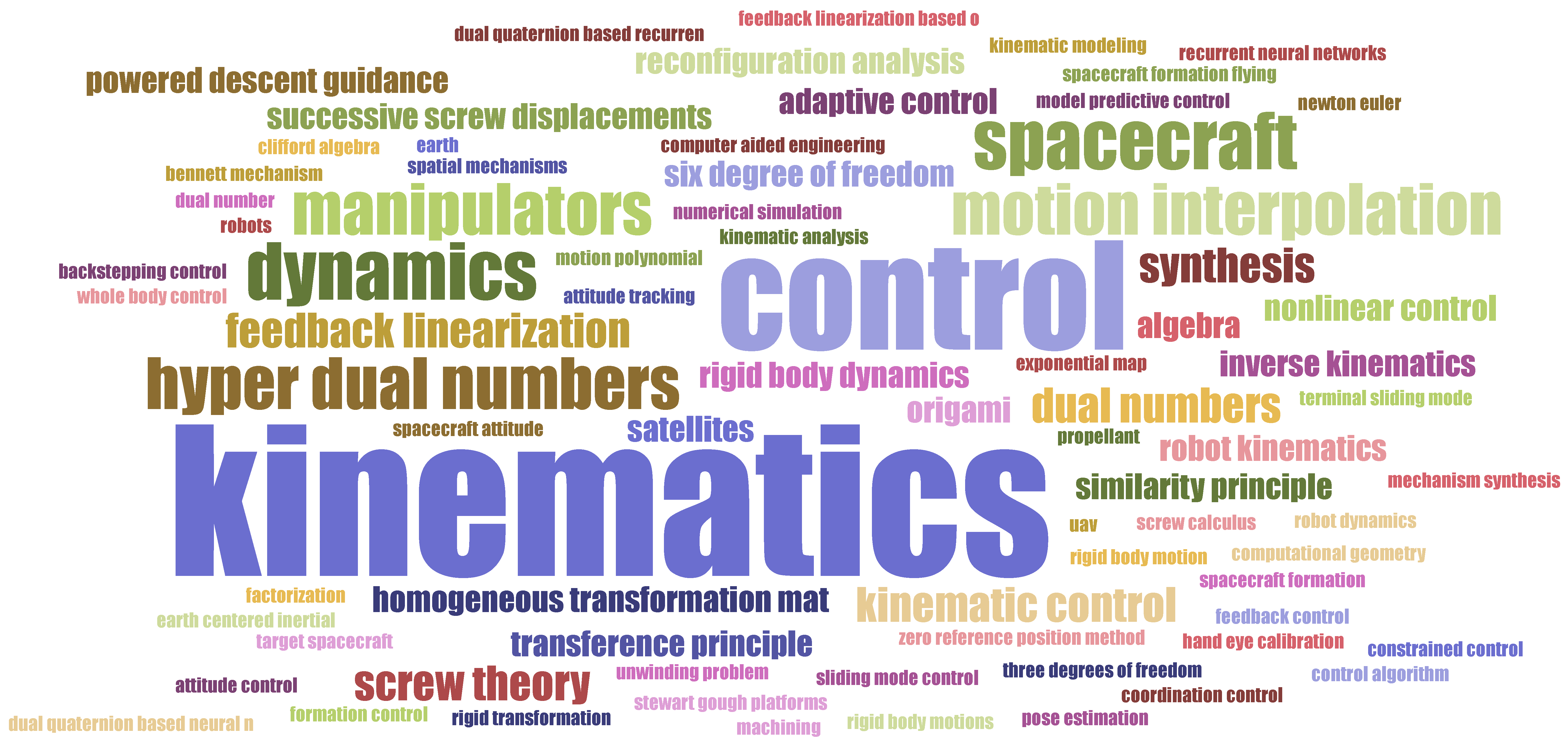
At last, we have two more figures: Figure 8, where we can see a wordcloud (made using https://www.jasondavies.com/wordcloud/; accessed on 23 February 2024) of the keywords from the articles cited in this work, and Figure 9: a bar graph showing the growth of articles containing dual quaternions in their title, from 1900 to 2023, according to Google Scholar (search was made for articles whose title contained one of the following words: “dual quaternion”, “dual-quaternion”, “dual quaternions”, “dual-quaternions”, “biquaternion” or “biquaternions”; accessed on 18 January 2024).

5.2. Free Rigid Bodies

The first application we explore in detail is free rigid bodies; we delve into its kinematics and dynamics, ending with the modeling of a free rigid body using dual quaternions.

5.2.1. Kinematics

In the case of free rigid bodies, all the kinematics of the body are compiled in a single dual quaternion. Consider the body initially aligned with an inertial reference frame, with its center of mass being the frame’s origin. Then, it undergoes a displacement (or several) which takes it to its current position. The dual quaternion q ^ ̲ is the operation that takes the body from its initial position to its current position, i.e., the dual quaternion represents the twist of the combined displacements that the body undertook.
Knowing q ^ ̲ = q ̲ + ε q o , the body’s orientation is given by the real quaternion q ̲ . The position is given by the pure translation associated with the operation as in Equation (35), i.e., t = 2 q o q ̲ * . As we consider the body initially aligned with the inertial frame, the initial position of the body is the actual origin of the frame; thus, the rotation q ̲ does not do any translation and the computed t is indeed the final position of the body.

5.2.2. Differential Kinematics of Rigid Bodies

To understand the differential kinematics using dual quaternions, it is advantageous to think of the displacements as if they were applied to a line. Consider first the more straightforward case of the rotation of a vector; using the same approach, the current vector v can be computed from the initial vector v by
v = q ̲ v q ̲ * .
From the study of classical mechanics, we know that the derivative of the vector v subject only to a rotational motion is given by
v ˙ = d v d t = ω × v ,
where ω is the angular velocity of the rotation.
The same equation in a quaternion framework takes the form
ω = 2 q ˙ ̲ q ̲ * or alternatively , q ˙ ̲ = 1 2 ω q ̲ .
Applying the Transference Principle to Equation (38), we arrive directly at (which is confirmed in [77])
ω ^ = 2 q ^ ˙ ̲ q ^ ̲ * = ω + ε ( t ˙ + t × ω ) .
As we can see, the resulting equation has the angular velocity in the primary part and the linear velocity in the dual part. The differential kinematics of a rigid body, both rotational and translational, are given by the following equation
ω ^ = 2 q ^ ˙ ̲ q ^ ̲ * or alternatively , q ^ ˙ ̲ = 1 2 ω ^ q ^ ̲ .
Notice that ω ^ is a twist: not a displacement twist, but a velocity twist. A displacement twist represents a combination of a rotation and a translation, whereas a velocity twist represents a combination of angular and linear velocity.
Equation (40) gives the core concept used in kinematic control, where the final pose of the body (given by q ^ ̲ ) is controlled by imposing a dual velocity to the motion, as seen in [78]. Also, articles that use of these kinematic concepts are the ones dealing with satellite proximity operations [47] and the relative pose of leader–follower formations [93].

5.2.3. Dynamics Using the Dual Inertia Operator

First, we need to introduce the concept of a wrench, which is the equivalent of a twist but instead of a pair of angular velocity and linear velocity, we have a pair of force and moment. We can write a wrench by
F ^ = F + ε ( t f × F + M o ) = F + ε M ,
where F ^ is the wrench, F is the force, t f × F is the moment generated by the force and M o is the pure moment in the direction of the force. Also, t f is the position of a point in the force’s line of action.
We will describe the dynamics of the body not in an inertial reference frame but in the body’s reference frame. To clarify the notation, we will denote a dual vector described in the body’s reference frame by a subscript b to the left, while keeping the ones described in the inertial frame without subscript. To relate the two reference frames, we use [1]
  b v ^ = q ^ ̲ * v ^ q ^ ̲ or v ^ = q ^ ̲   b v ^ q ^ ̲ * .
Using the body frame we can write the dual velocity [77] as
  b ω ^ = q ^ ̲ * ω ^ q ^ ̲ =   b ω + ε (   b t ˙ +   b ω ×   b t ) .
Back to the subject of the dynamics of rigid bodies, there are ways to obtain the equations of motion by using the wrench directly in the notation, as in [20]. But, they all turned out to be complicated and non-intuitive. An exception to this rule is the formulation derived by [43] and well developed in [127].
This formulation defines an operator d d ε , which acts like
d d ε ( a + ε a o ) = a o .
When we use both operators
ε + d d ε ( a + ε a o ) = a o + ε a ,
the effect is to swap the real and dual components.
The mass operator is defined by m ^ = m d d ε , i.e., the mass acts in a way to transform a vector in a rotor (line-vector). This behavior is cleverly explained by [127] by arguing that a vector attached to a mass has not only direction and magnitude, but also a position given by the mass, thus becoming a rotor. The inertia works the other way around, transforming a rotor in a vector.
Using those concepts, we can build a dual inertia operator as
I ^ = I ε + m d d ε ,
compute the dual momentum   b h ^ = I ^   b ω ^ and arrive at the dynamics by using Newton’s second law
  b F ^ = d d t   b h ^ = I ^   b ω ^ ˙ +   b ω × I ^   b ω ^ ,
which can be rewritten as
  b ω ^ ˙ = I ^ 1   b F ^   b ω × I ^   b ω ^ ,
where I ^ 1 = 1 m ε + I 1 d d ε .
This approach gives a very concise formulation to the dynamics, and although it is not the standard approach, it has received supporters [89,95].

5.2.4. Modeling of a Rigid Body

Given an applied system of forces, solving the equations returns the dual velocity and the associated dual quaternion; thus, the body’s position, orientation, linear velocity and angular velocity can be computed. The equations of motion form the following system of equations:
q ^ ˙ ̲ = 1 2 q ^ ̲   b ω ^
  b ω ^ ˙ = I ^ 1   b F ^   b ω × I ^   b ω ^ .
The above equations are well used in works treating modeling and controlling of rigid bodies using the dual quaternion approach. Abaunza et al. [48] uses the above equations to model and control an aerial manipulator, a quadcopter with a robotic arm, further validating experimental results. Wang and Yu [82] deduce the equations for general rigid-body motion dynamics and propose a feedback linearization controller to track a desired dual quaternion representing position and orientation.

5.3. Serial Mechanisms

In this section, we present the kinematics and differential kinematics of serial mechanisms. In addition, the concept of hyper-dual quaternions is introduced.

5.3.1. Direct Kinematics Using Successive Screw Displacements Method

The method of Successive Screw Displacements uses a reference configuration that eases the description of the mechanism and at which the rotations and displacements of the joints are considered zero-valued. The method was developed by Gupta [22,23] based on the Similarity Principle discovered by Roth [40] (and its companion article [41]). Gupta called it the Zero Reference Position Method, but we are adopting the name given by Tsai [128] as Successive Screw Displacements. This method allows for a simpler customized kinematic modeling of the mechanism at the expense of losing the standardization obtained by using Denavit–Hartenberg parameters (DH) (dual quaternions can also be used in a DH approach, Kim and Kumar [2] explain a method using the Left Operator).
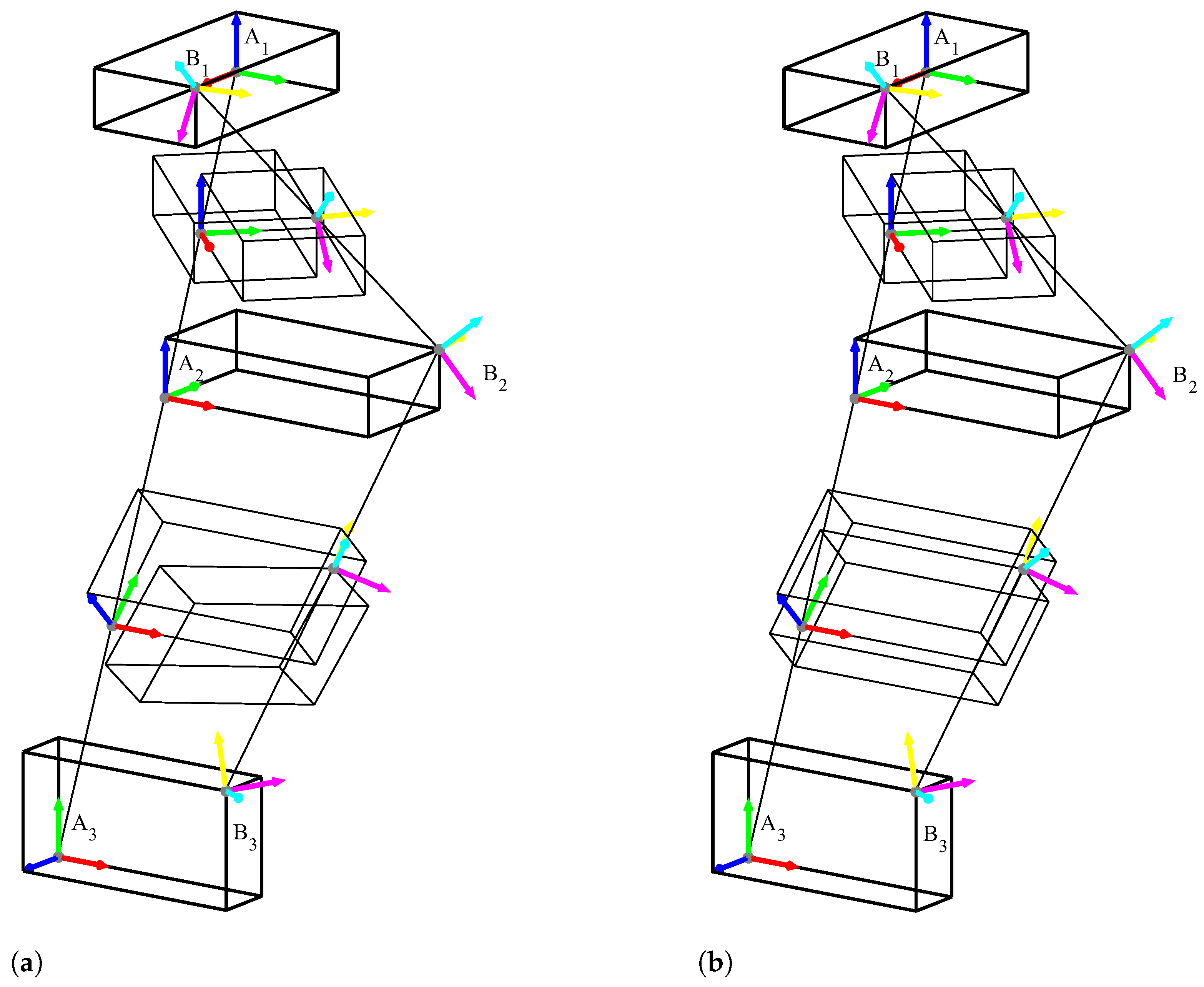
Following the description of the Successive Screw Displacement Method given by [129], first we choose the reference configuration, and we define a convenient fixed coordinate system. The convenient frame should make straightforward the description of the joints’ positions and directions when in the reference configuration. Figure 10 shows an example of reference configuration and convenient frame.
At this configuration and convenient frame, we can easily describe the joints’ axes’ directions and positions and compute the direct kinematics. As soon as the mechanism moves, those values are no longer true, so we need to consider the updated joints’ positions and orientations.
The method starts by building the reference configuration and convenient frame and using these to make a table of values identifying for each joint i: the direction of the joint s i , the position of the joint (or any point in the axis of the joint) p i , a rotation angle θ i and a displacement θ o i (forming the dual angle θ ^ i ). We use θ i = θ o i = 0 for the reference configuration, but, if they are variables, we leave them as θ i and/or θ o i .
Using the table of values we construct the following operator for each joint i:
q ^ ̲ i = cos ( θ ^ i 2 ) + sin ( θ ^ i 2 ) s ^ i ,
where s ^ i = s i + ε p i × s i , i.e., the axis of the joint in the reference configuration and convenient frame.
Note that the operators q ^ ̲ i are valid only for the reference configuration, where the axes on the q ^ ̲ i correspond to the real position and direction of the axes in the mechanism. Consider q ^ ̲   i to be the operators with the updated axes depending on the actual configuration. Joint 1 is connected to link 0, which is fixed, hence q ^ ̲   1 = q ^ ̲ 1 . Joint 2, on the other hand, is affected by the movements of joint 1, so that q ^ ̲   2 can be described by q ^ ̲   2 = q ^ ̲   1 q ^ ̲ 2 q ^ ̲ 1 * . Joint 3 depends on joint 1 and joint 2, so q ^ ̲   3 = q ^ ̲   2 q ^ ̲   1 q ^ ̲ 3 q ^ ̲ 1 * q ^ ̲ 2 * .
Actually, in a serial mechanism joint i is affected by every joint from 1 to i 1 , so for q ^ ̲   i we have
q ^ ̲   i = q ^ ̲   i 1 q ^ ̲   2 q ^ ̲   1 q ^ ̲ i q ^ ̲ 1 * q ^ ̲ 2 * q ^ ̲ i 1 * .
This seems complicated at first, but notice what happens when we compute the direct kinematics up to joint 2:
q ^ ̲   2 q ^ ̲   1 = ( q ^ ̲   1 q ^ ̲ 2 q ^ ̲ 1 * ) q ^ ̲   1 = q ^ ̲   1 q ^ ̲ 2 ( q ^ ̲ 1 * q ^ ̲   1 ) = q ^ ̲ 1 q ^ ̲ 2 ,
meaning the products simplify. Computing the direct kinematics up to joint 3,
q ^ ̲   3 q ^ ̲   2 q ^ ̲   1 = ( q ^ ̲   2 q ^ ̲   1 q ^ ̲ 3 q ^ ̲ 1 * q ^ ̲ 2 * ) q ^ ̲   2 q ^ ̲   1 = q ^ ̲   2 q ^ ̲   1 q ^ ̲ 3 ( q ^ ̲ 1 * q ^ ̲ 2 * q ^ ̲   2 q ^ ̲   1 ) = q ^ ̲   2 q ^ ̲   1 q ^ ̲ 3 ,
and substituting q ^ ̲   2 q ^ ̲   1 from Equation (52)
q ^ ̲   3 q ^ ̲   2 q ^ ̲   1 = q ^ ̲ 1 q ^ ̲ 2 q ^ ̲ 3 .
This behavior can be generalized to the direct kinematics up to joint n by
q ^ ̲   n q ^ ̲   2 q ^ ̲   1 = q ^ ̲ 1 q ^ ̲ 2 q ^ ̲ n .
We also need to define two more operations. We need an operation to go from a desired inertial (Ref0) frame to the convenient frame and an operation to go from the convenient frame to a desirable end-effector frame (Refe), we will call these operations q ^ ̲ 0 c and q ^ ̲ c e , respectively, and both are constant.
The end goal is to find the updated Refe from Ref0 and the joints configuration; this can be achieved by
Ref e = q ^ ̲ c e q ^ ̲ 1 q ^ ̲ n q ^ ̲ 0 c Ref 0 q ^ ̲ 0 c * q ^ ̲ n * q ^ ̲ 1 * q ^ ̲ c e * ,
Note that the general twist operator does not have the orthogonal and intersecting limitation of the left operator. Therefore, if we represent the reference frame by two orthogonal and intersecting lines (following [130], we can represent a frame by [ v ^ x v ^ y ] p , where v ^ x and v ^ y are two orthogonal lines intersecting at point p ), we can operate on both lines using the same operator, hence operating directly on the reference frame itself, which was performed in Equation (56). In fact, this reasoning allows for a further abstraction of the end-effector reference frame, representing it not by the two lines but by the transformation that takes the inertial frame and gives the end-effector frame.
Thus, the direct kinematics would not be the end-effector frame, but the transformation itself, which is the dual quaternion
q ^ ̲ = q ^ ̲ c e q ^ ̲ 1 q ^ ̲ n q ^ ̲ 0 c .
The Successive Screw Displacements method is used as a Screw Theory-based alternative to DH. Rocha et al. [129] compares both methodologies using homogeneous matrices, concluding that although the screw-based method seems more complex at first, it allows for great flexibility and the authors encourage its use. Perez and McCarthy [76] tackle the problem of kinematic synthesis, using the Successive Screw Displacements method to compute the direct kinematics of a mechanism at a finite set of key configurations in order to generate design equations that are further solved to find the geometrical parameters of the mechanism. Özgür and Mezouar [24] use a simpler, more straightforward version of the method, using of only one frame of reference.

5.3.2. Differential Kinematics

The dual velocity of the mechanism (more precisely of the end effector) is the combined effect of the dual velocity of all joints, and it can be computed by applying Equation (40) to the resulting dual quaternion of the direct kinematics of the mechanism. Applying it to Equation (55), but using only three joints for easier understanding, we have
ω ^ = 2 d d t q ^ ̲ 1 q ^ ̲ 2 q ^ ̲ 3 q ^ ̲ 1 q ^ ̲ 2 q ^ ̲ 3 * = 2 q ^ ˙ ̲ 1 q ^ ̲ 2 q ^ ̲ 3 + q ^ ̲ 1 q ^ ˙ ̲ 2 q ^ ̲ 3 + q ^ ̲ 1 q ^ ̲ 2 q ^ ˙ ̲ 3 q ^ ̲ 3 * q ^ ̲ 2 * q ^ ̲ 1 *
ω ^ = 2 q ^ ˙ ̲ 1 q ^ ̲ 1 * + q ^ ̲ 1 ( 2 q ^ ˙ ̲ 2 q ^ ̲ 2 * ) q ^ ̲ 1 * + q ^ ̲ 1 q ^ ̲ 2 ( 2 q ^ ˙ ̲ 3 q ^ ̲ 3 * ) q ^ ̲ 2 * q ^ ̲ 1 * ,
with q ^ ̲ i being constructed by Equation (50), s ^ i is constant-valued as it is defined in the reference configuration and convenient frame, both being fixed. So,
2 q ^ ˙ ̲ i q ^ ̲ i * = θ ^ ˙ i sin ( θ ^ i 2 ) + θ ^ ˙ i cos ( θ ^ i 2 ) s ^ cos ( θ ^ i 2 ) sin ( θ ^ i 2 ) s ^
2 q ^ ˙ ̲ i q ^ ̲ i * = θ ^ ˙ i sin ( θ ^ i 2 ) cos ( θ ^ i 2 ) + θ ^ ˙ i cos 2 ( θ ^ i 2 ) s ^ i + θ ^ ˙ i sin 2 ( θ ^ i 2 ) s ^ i θ ^ ˙ i cos ( θ ^ i 2 ) sin ( θ ^ i 2 ) s ^ i s ^ i .
It follows from the product rule of quaternions, Equation (21) and the conditions for being a line (Equation (12)) that s ^ i s ^ i = 1 + ε 0 . Thus, this results in
2 q ^ ˙ ̲ i q ^ ̲ i * = θ ^ ˙ i s ^ i .
Going back to Equation (59),
ω ^ = θ ^ ˙ 1 s ^ 1 + q ^ ̲ 1 θ ^ ˙ 2 s ^ 2 q ^ ̲ 1 * + q ^ ̲ 1 q ^ ̲ 2 θ ^ ˙ 3 s ^ 3 q ^ ̲ 2 * q ^ ̲ 1 * .
Note that the dual quaternions act to transform s ^ 1 , s ^ 2 and s ^ 3 to the same reference frame (Equation (42)), so we can write the above equation as
  b j ω ^ = θ ^ ˙ 1   b j s ^ 1 + θ ^ ˙ 2   b j s ^ 2 + θ ^ ˙ 3   b j s ^ 3 ,
where the before subscript b j is there to make explicit that the dual vectors must be the original s ^ i but transformed to the same reference frame. Generalizing the equation for n joints,
  b j ω ^ = i = 1 n n θ ^ ˙ i   b j s ^ i .
The quantities expressed by the dual velocity are linked to the frame origin. To be precise, the dual velocity in a frame gives us, in terms of values, the effect of the velocity computed relative to the origin of the frame.
Equation (65) can also be written using matricial formulation, which can be used as dual matrices with dual vectors and as ordinary matrices with vectors in R 6 (using Plücker coordinates), as in [129]. We find it advantageous to represent it by plucker coordinates, which allows us to separate the dual velocity θ ^ ˙ s ^ into θ ˙ s ^ + ε θ ˙ o s ; these would be given in Plücker coordinates as
θ ^ ˙ s ^ = θ ˙ s s o + θ ˙ o 0 s .
We can write the differential kinematics as
vec ω ^ = s 1 0 s 2 0 s n 0 s o 1 s 1 s o 2 s 2 s on s n θ ˙ 1 θ ˙ o 1 θ ˙ n θ ˙ o n
vec ω ^ = J θ ˙ ,
where J is the Jacobian, θ ˙ is a vector with joint variables derivative and vec is a function that receives a dual vector and transforms it in a column vector with dimension 6. It assigns the primary part of the dual vector to the first three components and the dual part to the last three.
Using this matricial formulation, we can easily specialize joints as revolute by excluding θ ˙ o or prismatic by excluding θ ˙ , also excluding the respective columns of the matrix. The inverse differential kinematics can be computed, whenever J is invertible, by θ ˙ = J 1 vec ω ^ .

5.3.3. Differential Kinematics Using Hyper-Dual Quaternions

The concept of hyper-dual numbers is very recent [131] and consists of using two different dual generators like ε 1 and ε 2 . Using those a general hyper-dual number takes the form
a ˇ = a 0 + ε 1 a 1 + ε 2 a 2 + ε 1 ε 2 a 3 ,
where the over upside-down hat indicates a hyper-dual entity.
Another way to look at hyper-dual numbers is as nested dual numbers. Keeping the traditional ε generator and adding a second one as ε ˇ , we can write a hyper-dual number as
a ˇ = a ^ 1 + ε ˇ a ^ 2 = ( a 1 + ε a o 1 ) + ε ˇ ( a 2 + ε a o 2 ) .
We will define the quantity that is not being multiplied ε ˇ as the hyper-primary part of the hyper-dual number, while the other part is the hyper-dual part.
This approach uses the “automatic differentiation” property of dual numbers. By applying hyper-dual number matrices [35,36] and hyper-dual quaternions [38], the authors therein could simultaneously compute the kinematics and differential kinematics of rigid bodies and serial mechanisms. The regular kinematics appears in the hyper-primary part, while the differential kinematics appears in the hyper-dual part. According to these authors, obtaining the Jacobian matrix and its derivative is possible without performing differentiations. In these papers, the dynamics are also computed using a hyper-dual approach through the extension of the dual inertia operator.
In [37], usual trigonometric identities are proven using hyper-dual numbers, and also the dot and cross products of hyper-dual vectors are proven to yield the same simple formula but with hyper-dual quantities. The authors called those proofs “an extension of the Transference Principle to hyper-dual numbers”.
Consider a hyper-dual quaternion operator defined as q ˇ = cos ( α ˇ 2 ) + sin ( α ˇ 2 ) s ^ , where q ˇ is the hyper-dual quaternion, α ˇ is a hyper-dual angle and s ^ is a unit dual vector representing the axis of the screw operation. This result can be rewritten as
q ˇ = q ^ + ε ˇ q ^ ˙ = q ^ + ε ˇ 1 2 ω ^ q ^ .
When combining three operations, we obtain
q ˇ e = q ˇ 1 q ˇ 2 q ˇ 3 = q ^ 1 q ^ 2 q ^ 3 + ε ˇ 1 2 ( ω ^ 1 q ^ 1 q ^ 2 q ^ 3 + q ^ 1 ω ^ 2 q ^ 2 q ^ 3 + q ^ 1 q ^ 2 ω ^ 3 q ^ 3 ) .
In order to see that the hyper-dual part really contains the differential kinematics, let us compute the dual velocity by ω ^ e = 2 q ^ ˙ e q ^ e * ,
ω ^ e = ω ^ 1 + q ^ 1 ω ^ 2 q ^ 1 * + q ^ 1 q ^ 2 ω ^ 3 q ^ 2 * q ^ 1 * ,
where we could substitute ω ^ i by θ ^ i s ^ i , as seen in Equation (62).
Equation (73) is in accordance with the development of the differential kinematics of serial mechanisms, so we are computing both the kinematics and differential kinematics all at once.
Hyper-dual quaternions can potentially compute both the kinematics and differential kinematics in a single entity. Once we define the initial hyper-dual quaternions, the computation takes place as if we were only dealing with the kinematics, as the dual structure incorporates the algebra related to the differential of functions. For example, if we multiply two hyper-dual quaternions, the hyper-dual part will be the derivative of the product of two functions. The result of this derivative operation will appear in the hyper-dual part as if we had used the product rule of differentiation:
q ˇ 1 q ˇ 2 = q ^ 1 + ε ˇ q ^ ˙ 1 q ^ 2 + ε ˇ q ^ ˙ 2 = q ^ 1 q ^ 2 + ε ˇ q ^ ˙ 1 q ^ 2 + q ^ 1 q ^ ˙ 2 .

5.4. Parallel Mechanisms

Parallel mechanisms are presented in this section, the direct and inverse kinematics of this type of mechanism are explored.

Kinematics of Parallel Mechanisms

In a parallel mechanism, there is more than one kinematic path to go from the base to the platform. For example, if link 0 is the base and link e the platform, there can be a path 0 1 2 3 e and a path 0 4 5 6 e that both start in the base and end in the platform. Then, those paths can be combined in a kinematic loop, which would be a path that starts and ends at the same link, like 0 1 2 3 e 6 5 4 0 .
For each independent kinematic loop, we can form one loop equation. Consider q ^ ̲   1 , the dual quaternion that takes from Ref0 to Refe using path 0 1 2 3 e , and q ^ ̲   2 , the dual quaternion that does the same job using path 0 4 5 6 e . Both quaternions must be equal, so the loop equation would be q ^ ̲   1 q ^ ̲   2 = 0 . Note that both q ^ ̲   1 and q ^ ̲   2 depend on the active and passive joints variables, so their numerical value cannot be computed as the passive joints variables are unknown. For n loops, we have n + 1 distinct paths taking from Ref0 to Refe, so we can write [132]
q ^ ̲   1 q ^ ̲   i = 0 , i = 2 , , n + 1 .
Taking all the loop equations as Equation (75), we can build a system of equations and use a numerical method to solve it to obtain the values of the passive joints’ variables. Once we have those we can compute the direct kinematics, i.e., the numerical value of any dual quaternion q ^ ̲   i .
Yang and Freudenstein [19] use a similar approach to generate the loop equation of a spatial four-link mechanism but using the left operator quaternion.
An interesting approach to the direct kinematics of a class of six-degrees-of-freedom parallel robots is presented in [27]. Those 6-DOF parallel robots can be fully actuated or redundant, and their passive joints are designed as compound hinges whose axes intersect at a point, universal and spherical joints are included. The dual quaternion formulation allowed the authors to obtain the direct kinematics in a quadratic form, which can be exploited in numerical optimization methods. Taking advantage of the quadratic form, an algorithm is derived that solves every iteration (of the direct kinematics computation) on average in 0.2187 milliseconds, whereas a traditional Newton method takes 14.25 milliseconds.
The inverse kinematics of parallel mechanisms is generally simple, at least simpler than direct kinematics. The problem consists in finding the joint variables values given the pose of the mobile platform. Considering the pose given by the dual quaternion q ^ ̲ , we would have, for each independent kinematic chain going from the base to the platform,
q ^ ̲   i = q ^ ̲ , i = 1 , , n + 1 ,
where n is the number of kinematic loops. We can solve each equation in Equation (76) alone to compute the joint variables in the respective kinematic chain. At the end we will have computed all joint variables.

5.5. Control

Before starting the study of control using dual quaternions, we need to provide a few concepts. The first is the concept of the tracking error. Consider two dual quaternions, q ^ ̲ representing the actual pose and q ^ ̲ d representing the desired pose. Their difference can be evaluated by two forms [18]
q ^ ̲ e r = q ^ ̲ q ^ ̲   d 1 = q ^ ̲ q ^ ̲ d *
q ^ ̲ e l = q ^ ̲   d 1 q ^ ̲ = q ^ ̲ d * q ^ ̲ ,
where q ^ ̲ e r is called the right-invariance error and q ^ ̲ e l is called the left-invariance error. The right-invariance error is better suited to work with the inertial frame, while the left-invariance error is better suited to work with the body frame. This can be shown when we compute the error derivative, which results in
q ^ ˙ ̲ er = 1 2 ω ^ er q ^ ̲ e r q ^ ˙ ̲ el = 1 2 q ^ ̲ e l   b ω ^ el ,
where ω ^ is the dual velocity of the system, ω ^ d is the dual velocity of the desired pose, ω ^ er = ω ^ q ¯ ^ er ω ^ d q ¯ ^ er * is the dual velocity associated with the right error dynamics and   b ω ^ el =   b ω ^ q ¯ ^ el *   b ω ^ d q ¯ ^ el   is the dual velocity associated with the left error dynamics. Other error metrics exist, like in [46].
Two other important concepts that appear a lot in control involving dual quaternions are the exponential and logarithm of dual quaternions. Those are connected with the theory of Lie Groups and Lie Algebras. The exponential of a dual quaternion can be computed by
exp ( q ^ ) = k = 0 q ^ k k ! = 1 + q ^ + q ^ 2 2 ! + q ^ 3 3 ! +
Thus, applying the twist θ ^ s ^ ̲ as a dual quaternion in the above equation gives
exp ( θ ^ s ^ ̲ ) = 1 + θ ^ s ^ ̲ θ ^ 2 2 ! θ ^ 3 s ^ ̲ 3 ! + θ ^ 4 4 ! + θ ^ 5 s ^ ̲ 5 ! θ ^ 6 6 ! θ ^ 7 s ^ ̲ 7 ! exp ( θ ^ s ^ ̲ ) = 1 θ ^ 2 2 ! + θ ^ 4 4 ! θ ^ 6 6 ! + + s ^ ̲ θ ^ θ ^ 3 3 ! + θ ^ 5 5 ! θ ^ 7 7 ! + exp ( θ ^ s ^ ̲ ) = cos ( θ ^ ) + sin ( θ ^ ) s ^ ̲ .
The exponential function applied to a twist gives the dual quaternion operation associated with that twist. The logarithm function, being the inverse function of the exponential, has the inverse effect, i.e., when given a dual quaternion operator, it returns the twist associated with the operation,
ln cos ( θ ^ ) + sin ( θ ^ ) s ^ ̲ = θ ^ s ^ ̲ .
Considering a general twist operator which works with half angles, we have the result of the logarithm of q ^ ̲ = cos ( θ ^ 2 ) + sin ( θ ^ 2 ) s ^ ̲ is ln q ^ ̲ = 1 2 θ ^ s ^ ̲ . Also, the qt twist operator q ^ ̲ = q ̲ + ε p q ̲ 2 , where q ̲ = cos ( θ 2 ) + sin ( θ 2 ) s ̲ , is associated with a twist corresponding to a rotation of θ / 2 around an axis with direction s ̲ going through the origin followed by a translation p / 2 . Thus, the logarithm of the dual quaternion q ^ ̲ is given by
ln q ^ ̲ = 1 2 θ s ̲ + ε 1 2 p .

5.5.1. Kinematic Control

Kinematic control aims to control the position and orientation of a system by imposing its linear and angular velocity. In the case of the kinematics given by a dual quaternion, kinematic control involves controlling the pose q ^ ̲ by using the equation
q ^ ˙ ̲ = 1 2 ω ^ q ^ ̲ ,
where the controller will act by imposing the dual velocity ω ^ .
In [133], a control law for the regulation problem is presented as
ω ^ = 2 k ln q ^ ̲ , k > 0 ,
this results in
q ^ ˙ ̲ = k ln q ^ ̲ q ^ ̲ .
To prove the stability of the proposed controller, the author considers a new norm
N ( q ^ ̲ ) = 2 | | vec ( ln q ^ ̲ ) | | = 2 vec ( ln q ^ ̲ ) · vec ( ln q ^ ̲ ) ,
where the function vec takes a dual vector and transforms it into a real vector, as defined after Equation (67).
It is used as a candidate Lyapunov function W = 1 2 N 2 ( q ^ ̲ ) . Differentiating the previous equation gives
d d t W = 2 vec ( ln q ^ ̲ ) · 2 d d t vec ( ln q ^ ̲ ) = 2 vec ( ln q ^ ̲ ) · vec ( ω ^ )
d d t W = 2 vec ( ln q ^ ̲ ) · [ 2 k vec ( ln q ^ ̲ ) ] = k W ,
where the passage to the last equality in Equation (88) is proved as a theorem in the article. We conclude that Lyapunov function converges to zero exponentially and so the control law stabilizes the system, taking ln q ^ ̲ to zero, which is equivalent to
q ^ ̲ ± 1 .
Note that there are two possible equilibrium points given by Equation (90). This multi-equilibrium emerges because the dual quaternions q ^ ̲ and q ^ ̲ represent the same pose. The phenomenon is called “the unwinding problem”, and it is a problem because an initial state can go to the furthest equilibrium instead of the closest, which is undesirable. To handle the unwinding problem, ref. [82] defines an extra parameter λ according to the proximity of the initial state and the equilibrium points given by
λ = 1 , if q ^ ̲ e 1 ( t ) 0 1 , otherwise ,
where q ^ ̲ e 1 ( t ) is the first element in q ^ ̲ e ( t ) , i.e., the scalar component of the real quaternion. With regulatory control, q ^ ̲ e ( t ) is constructed by using q ^ ̲ d ( t ) 1 . Introducing this added parameter, the control law becomes
ω ^ = 2 k ln ( λ q ^ ̲ ) .
Then, the system will go to the nearest equilibrium using the above equation and given arbitrary initial conditions.
For the tracking problem, the idea is to use ω ^ to make q ^ ̲ go to q ^ ̲ d . This is accomplished by getting the error to ± 1 , or the logarithm of the error to zero. Han et al. [133] use a right invariant error as given in Equation (77), so the control law for the tracking problem can be computed as
ω ^ = 2 k ln q ^ ̲ e + q ^ ̲ e ω ^ d q ^ ̲ e * ,
this leads (from Equation (79)) to
q ^ ˙ ̲ e = k ln q ^ ̲ e q ^ ̲ e .
It is easy to test this control law using an analogous candidate Lyapunov function. The result is q ^ ̲ e ± 1 , which is equivalent to q ^ ̲ ± q ^ ̲ d , so the pose of the system q ^ ̲ tracks the desired pose q ^ ̲ d . The parameter λ in Equation (91) avoids the unwinding problem.
The authors remark that by using this dual quaternion approach it is possible to perform a kinematic control keeping intact the natural coupling between rotational and translational motion in a rigid body. Also, using a different gain for the real and dual part of the dual velocity, it is possible to adjust the importance given by the control to the rotation and translation separately.
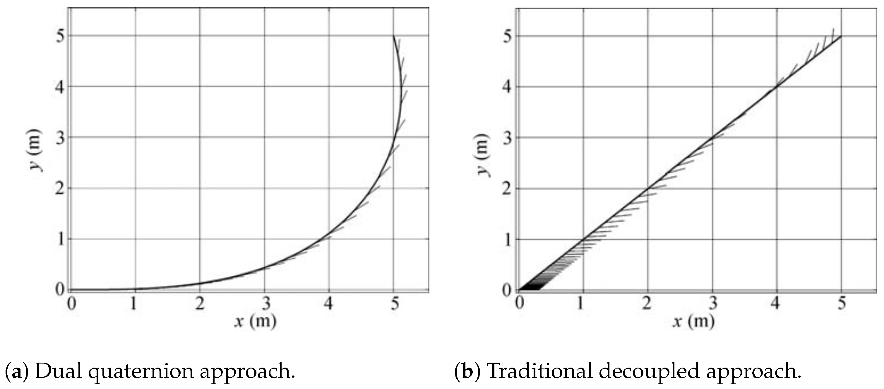
To show the differences in results, the authors compare the developed control to a traditional approach that decouples the rotational and translational motion, applying both on an omnidirectional mobile robot. The pose of the robot is defined by three parameters ( x , y , α ) where ( x , y ) corresponds to a point in the plane and α gives the orientation of the vehicle in relation to the x axis. The results of both approaches for taking the robot from ( 5 , 5 , π 2 ) to ( 0 , 0 , 0 ) are shown in Figure 11.
According to the authors, if synergy between orientation and position is important, the dual quaternion approach should be preferred, like in a robot soccer game. Notice that, in the dual quaternionic case, the robot’s trajectory is linked to its orientation, whereas in the traditional approach it just goes linearly to the endpoint.
There are more contributions to kinematic control using dual quaternions: ref. [18] compares the computational efficiency of the logarithm control law using dual quaternions and homogeneous matrices, and the result is much favorable to dual quaternions. Kussaba et al. [81] tackle the chattering caused by the discontinuous solutions (for example, Equation (91)) to the unwinding problem, proposing a switching kinematic controller with hysteresis for the rigid-body stabilization. Wang and Yu [79] use a left-invariant error like in Equation (78) and proposes a generalization of the kinematic control developed in this section to a PID scheme using
  b ω ^ e = 2 k ^ p ln q ^ ̲ e + k ^ p ( ln q ^ ̲ e ) + k ^ i ln q ^ ̲ e d t .

5.5.2. Feedback Linearization

Wang and Yu [82] propose a feedback linearization control using the dynamic equations of a rigid body and of the tracking error. The authors separate the equation into two parts, one containing the external torques and forces and one that does not. This is shown as
  b ω ^ ˙ = L ^ + U ^ ,
where U ^ is the part that contains the external torques and forces and it will be used as the control input and L ^ contains the remaining terms. So, the equations of motion for the system are given by
q ^ ˙ ̲ = 1 2 q ^ ̲   b ω ^   b ω ^ ˙ = L ^ + U ^ .
Next, the authors obtain analogous equations of motion but for the error. The error is defined as a left invariant error of form q ^ ̲ e = q ^ ̲ d * q ^ ̲ , which gives the derivative q ^ ˙ ̲ e = 1 2 q ^ ̲ e   b ω ^ e . The error dual velocity is given by
  b ω ^ e =   b ω ^ q ^ ̲ e *   b ω ^ d q ^ ̲ e .
Taking the derivative of Equation (98) gives
  b ω ^ ˙ e =   b ω ^ ˙ q ^ ̲ e *   b ω ^ ˙ d q ^ ̲ e ( q ^ ̲ e *   b ω ^ d q ^ ̲ e ) ×   b ω ^ e   b ω ^ ˙ e = L ^ q ^ ̲ e *   b ω ^ ˙ d q ^ ̲ e ( q ^ ̲ e *   b ω ^ d q ^ ̲ e ) ×   b ω ^ e + U ^ .
At last, we can write the error model equations as
q ^ ˙ ̲ e = 1 2 q ^ ̲ e   b ω ^ e
  b ω ^ ˙ e = L ^ q ^ ̲ e *   b ω ^ ˙ d q ^ ̲ e ( q ^ ̲ e *   b ω ^ d q ^ ̲ e ) ×   b ω ^ e + U ^ .
The authors propose the following control law
U ^ = 2 k ^ p ln q ^ ̲ e k ^ v   b ω ^ e L ^ + q ^ ̲ e *   b ω ^ ˙ d q ^ ̲ e + ( q ^ ̲ e *   b ω ^ d q ^ ̲ e ) ×   b ω ^ e ,
which consists of two parts: a proportional and derivative feedback given by the two first terms and a feedforward compensation given by the other terms. These last terms have the intention of compensating the non-linearities of the system as is typical of a feedback linearization control, and the resulting dynamics in closed loop are given by
q ^ ˙ ̲ e = 1 2 q ^ ̲ e   b ω ^ e
  b ω ^ ˙ e = 2 k ^ p ln q ^ ̲ e k ^ v   b ω ^ e .
To deal with the unwinding problem, the author adds the parameter λ (Equation (91)) to the term 2 k ^ p ln q ^ ̲ e , changing it to 2 k ^ p ln ( λ q ^ ̲ e ) . At the end, the proposed controller converges from ( q ^ ̲ e ( t ) ,   b ω ^ e ( t ) ) to ( ± 1 , 0 ) asymptotically, thus making the system pose follow the desired pose.
A very similar control law, almost identical (but that actually came first), is proposed by [133]. Both works remark on the ability of the control law to handle the coupling and achieve harmony between rotation and translation. Adaptations to the controller developed in this section are made by [83,85] to use it in a whole-body application consisting of a robotic arm mounted in an omnidirectional vehicle, and shows the experimental results of the applied control. Antonello et al. [84] uses a Feedback Linearization controller for the maneuver regulation of a free rigid-body.

5.5.3. Other Control Strategies Using Dual Quaternions

In [87,88], the authors apply MPC and dual quaternions to an autonomous landing control of a spacecraft. They justify the used strategy by saying that the task requires a coupling of position and orientation through constraints; for example, it is required that the spacecraft onboard vision sensors maintain the line-of-sight with the surface target during the descent phase. Such constraint is affected by the spacecraft orientation and position during landing. Thus, dual quaternions are a better option as they treat rotational and translational dynamics as one. In addition, MPC is used to add the task constraints into the controller formulation.
In the works of Filipe and Tsiotras [47,89], a dual quaternion-based Adaptive Control is developed and applied for satellite proximity operations in which no information about the mass and inertia matrix of the body is needed; instead, the controller can identify those parameters. The authors remark that many attitude-only quaternion-based controllers can be extended to position and attitude by using dual quaternions. The result may also maintain similar properties (e.g., stability, adaptivity).
One example of such extensions is [93], which extends a backstepping controller from quaternion to dual quaternion applying it to the relative pose stabilization of a follower spacecraft and a leader spacecraft. Backstepping controller is also used in [94].
Dong et al. [91] develop a fault-tolerant Sliding Mode controller using dual quaternions for a target-pursuer spacecraft tracking. The faults can be partial or total actuator power loss, actuator offset and locking. The controller is used in a simulation showing promising results. Huang et al. [92] propose a formation control whose formation error is controlled through a Sliding Mode controller and one term is added for collision avoidance using Artificial Potential Function. Mas et al. [118] also develop a formation control: the authors use a dual quaternion approach in a leader–follower configuration of a ground vehicle being escorted by an aerial one. The formation control is validated experimentally.

5.6. Rigid-Body Motion Interpolation

Given key configurations of an object to find an approximate continuous motion that goes from the previous key configuration to the next is the problem of motion interpolation [44]. Some properties desired in motion interpolation are constant speed, shortest path and coordinate system invariance.
Following the definitions in [61], when a motion has a constant speed, its rotation angle and/or distance of translation varies linearly regarding to the parameter t of time. The shortest path property means that the motion is a rotation about a fixed axis with the smallest angle and/or a translation along a direction with the smallest distance. A coordinate system invariance motion requires the motion to be the same independently of the coordinate frame in which it is represented.
Generally, the interpolation of an arbitrary motion is dealt wiht by separating the rotational motion and the translational motion. The translational motion is simpler and can be interpolated using linear interpolation, which has all the above-mentioned desired properties.
The case of interpolating orientation is more complex. One way for it to be achieved is by linearly interpolating Euler angles, but those lose all the three desired properties of interpolations [63]; this behavior is illustrated in Figure 12a. If we try to linearly interpolate all the components of a rotation matrix, the result can sometimes not be an orthogonal matrix and can even be a singular one [61]. A way of interpolating orientation based on quaternions was developed by Shoemake and it is called slerp (short for Spherical Linear Interpolation). This has the three properties of the shortest path, constant speed and coordinate invariance. Its formulation is given by
q ̲ ( t ) = slerp ( q ̲ i , q ̲ i + 1 ; t ) = q ̲ i ( q ̲ i 1 q ̲ i + 1 ) t , 0 t 1 ,
where q ̲ ( t ) is the parametrized interpolated rotation and q ̲ i is the orientation of the configuration i. Remember that q ̲ i 1 = q ̲ i * , so the result of the slerp is actually q ̲ i ( q ̲ i * q ̲ i + 1 ) t .
Note that when we are dealing with orientation (and later when dealing with translation and orientation) the shortest path is no longer a straight line. Although pure translation can be described in an Euclidian Space, rotation cannot be described in such space. An orientation can be described as a point in a 3D sphere in the fourth dimension (as in the case of representing orientation by a unit quaternion), where each point in the sphere corresponds to one possible orientation (actually, the whole sphere is a double cover for the possible orientations). So, in this 3D sphere, the shortest path is a curved path along this sphere, which is a geodesic path.
Although the linear interpolation for translation and slerp for orientation both have the desired properties, the decomposition of rotation and translation inevitably depends on the coordinate system, so the property of coordinate independence is lost [61]. In addition, [63] states that the in-between poses are not unique when position and orientation are interpolated separately because superimposing position and rotation is non-linear. Figure 12b illustrates a motion interpolation using slerp for orientation and linear interpolation for translation.
A pose interpolation obtained by the dualization of the slerp is called sclerp (short for Screw Linear Interpolation) and is given by
q ^ ̲ ( t ) = sclerp ( q ^ ̲ i , q ^ ̲ i + 1 ; t ) = q ^ ̲ i ( q ^ ̲ i 1 q ^ ̲ i + 1 ) t , 0 t 1 ,
where q ^ ̲ ( t ) is the parametrized interpolated pose and q ^ ̲ i is the pose of the configuration i. Remember that q ^ ̲ i 1 = q ^ ̲ i * , so the result of the sclerp is actually q ^ ̲ i ( q ^ ̲ i * q ^ ̲ i + 1 ) t . To understand how sclerp performs the motion first notice that q ^ ̲ ( 0 ) = q ^ ̲ i ( q ^ ̲ i * q ^ ̲ i + 1 ) 0 = q ^ ̲ i and q ^ ̲ ( 1 ) = q ^ ̲ i q ^ ̲ i * q ^ ̲ i + 1 = q ^ ̲ i + 1 . In the case of a non-integer power, we need to use the concepts of exponential and logarithm from Section 5.5. If we apply the logarithm to a quaternion power
ln q ^ ̲ t = t ln q ^ ̲ = 1 2 t θ ^ s ^ ̲ ,
then applying the exponential, we obtain back q ^ ̲ t as
q ^ ̲ t = exp ln q ^ ̲ t = cos ( t θ ^ 2 ) + sin ( t θ ^ 2 ) s ^ ̲ .
The term ( q ^ ̲ i * q ^ ̲ i + 1 ) in the sclerp defines an operation of the type q ^ ̲ = cos ( θ ^ 2 ) + sin ( θ ^ 2 ) s ^ ̲ which is associated with the twist that takes the pose q ^ ̲ i to the pose q ^ ̲ i + 1 . The axis of the operation remains fixed and we interpolate by changing linearly the dual angle from 0 to θ ^ / 2 . The resulting interpolation has the properties of shortest path, constant velocity and coordinate invariance.
Although the common way to express a sclerp is using Equation (106), ref. [44] found an alternative expression by
sclerp ( q ^ ̲ i , q ^ ̲ i + 1 ; t ) = sin ( ( 1 t ) α ^ ) sin ( α ^ ) q ^ ̲ i + sin ( t α ^ ) sin ( α ^ ) q ^ ̲ i + 1 ,
where α is the dual angle between the axes of q ^ ̲ i and q ^ ̲ i + 1 .
The sclerp can also be used to interpolate between over two poses by treating every two successive poses separately. Still, the result is a C 0 interpolation, meaning that it would be continuous for the key poses but may not be for higher-order differentials, i.e., sudden changes in velocity can happen along with the motion. When dealing with more than two key configurations, at least a C 1 interpolation is desirable, because it connects the poses making the velocity continuous along with the interpolation. To obtain a C 1 interpolation both [44,63] use an extension of the De Casteljau algorithm to build a Bézier-like interpolation of sclerps.
Figure 13 shows the difference of sclerp and the C 1 dual quaternion interpolation, notice that in sclerp when going through the second key frame there is a sudden change in the tangent line, indicating velocity, while in the C 1 there is a smooth transition.
Allmendinger et al. [63] show how to properly compute the control points of the C 1 interpolation of motion to obtain the desired velocities in the key frames of the motion, if those are not known. The article also shows how to tune the motion using different parameters or sets default values of those parameters to automatically compute the control points. In Ge and Ravani [45], the authors develop a Bézier interpolation that has Bernstein polynomial basis and allows for subdivision of the motion.
An interesting application of this subject is shown in [62]. According to the authors, new non-invasive kinematic assessment techniques provide improved insight on joint biomechanics but at the expense of higher radiation exposure to the patient. So, the article proposes to minimize the radiation by exposing the patient only to obtain key configurations of the joints and using dual quaternion interpolation to reconstruct the motion. One analysis in the reconstruction of 3D spine kinematics sampling the data from a full range of motion data showed that using only 0.36 % of the original data, it was possible to reconstruct the original motion with less than 1 % of normalized root-mean-squared error and less than 2 % normalized maximum error.

5.7. Others Applications

Other noteworthy applications touched upon are presented below.

5.7.1. Kinematic Synthesis

Perez and McCarthy [76] present a methodology to determine the structural parameters for designing a robotic system. The authors’ goal in kinematic synthesis is to design a serial chain that can reach a prescribed set of task positions. These positions provide a discrete approximation of the workspace of the desired chain.
The methodology used consists first in computing the direct kinematics of a desired mechanism by knowing its topology, i.e., the joints’ types and order (like RPRP), and using Successive Screw Displacements (Section 5.3.1). That being completed, we will have the direct kinematic equation of the mechanism as a function of the structural parameters and joint variables values. The next step is to compute the maximum number of task positions we can give for the system; this is carried out by evaluating the number of joints, the types of the joints and any additional geometric constraint we might want to impose. After that, we select the needed task positions.
Having the task positions and the computed direct kinematics, we can generate the design equations of the system by equating them. For each dual quaternionic identity, we have six independent equations. This set of equations forms the design equations of the system.
Perez and McCarthy [76] conduct a process called Inverse Kinematics Elimination to eliminate the values of the joint variables and solve a simpler system of equations involving only the structural parameters. The authors apply the developed methodology to the kinematic synthesis for two robots, an RPRP and an RPC. In [134], the same authors develop a similar methodology, but using Clifford algebra exponentials.

5.7.2. Processing Visual Data

The problem of using dual quaternions in identifying the position and orientation of an object using visual data, which can be provided by measured point features in the object’s surface and/or measured unit direction vectors features from the object, is tackled in [56]. Examples of point features might be any combination of the corner points, masked points or center of a sphere and unit vector features include surface normals and edge directions.
Those points and vectors are then compared with the ones obtained by a model of the object. If we consider   b p i as a point feature described in the object frame, which is known, the same point in the inertial frame can be described by
p i = 2 q o q ̲ * + q ̲   b p i q ̲ * .
The point p i should be approximately the measured point p m i , so we can compute an error from modeled point to measured point as p e i = p i p m i , where p e i is the position error.
When dealing with unit direction vectors features, the modeled is given by n i = q ̲   b n i q ̲ * and the error between the modeled and the measured vectors ( n m i ) is n e i = n i n m i , where n e i is the vector error.
The idea is to build a cost function using the square of the errors as
E = i = 1 k γ i | | n e i | | 2 + i = 1 l δ i | | p e i | | 2 ,
where γ i and δ i are weighting factors. Equation (111) can be optimized to obtain the dual quaternion q ^ ̲ = q ̲ + ε q o that minimizes the cost function value. This yields a quadratic function of q ̲ and q o , which can be exploited by optimization techniques.
Walker et al. [56] use a matricial approach to the quaternion algebra, defining quaternions as four-dimensional vectors and special matrices to perform the quaternionic multiplications. The resulting method was compared with a Singular Value Decomposition (SVD) method by simulation, showing a better accuracy and very good computational performance with the computational cost increasing linearly with the number of samples.
Qiao et al. [57] use a similar method to identify the relative position and attitude of two spacecrafts during the rendezvous and docking phase, in which the chaser spacecraft gets closer to the target spacecraft for docking and needs to know precisely the relative pose between the two by relying primarily on measured visual data.
Another application of dual quaternions involving visual data is presented in [59], in which the authors use dual quaternions to identify the relative position and orientation of left and right in stereo-pair images by presenting the coplanarity equation based on dual quaternions.
Daniilidis [70] uses dual quaternions and screw theory to perform a hand–eye calibration. In a robot with a camera mounted, the hand–eye calibration deals with how to relate the frame of the camera to the frame of the robot. In this way, the visual data from the camera can be used to correctly positioning a gripper, for example. The author also compares the developed method experimentally with two others, showing superior results for the dual quaternionic method, which is attributed to the fact that the dual quaternionic method solves rotation and translation simultaneously and to the better modeling of the problem achieved using Screw Theory.
Also, using a similar methodology, refs. [58,60] use dual quaternions in the application of Point Cloud Registration which consists of reconstructing complex geographical entities, requiring several stations to acquire the detailed point cloud fully. This results in a need to register point clouds from different stations to obtain an integrated point cloud.

5.7.3. Estimation and Navigation

Filipe et al. [101] propose an Extended Kalman Filter (EKF) for spacecraft pose estimation using dual quaternions. The filter was developed as a dual extension of an existing attitude-only quaternionic EKF. Using dual quaternions allows for the simultaneous estimation of attitude and position. In contrast, traditional methods compute first the attitude, then the position. This carries to the position any error in the attitude. Other pose estimators have been proposed, like Moving Horizon Estimator [115], 6-DOF observer [98] and Particle Filter [116].
The problem of strapdown inertial navigation system (INS) is tackled by [77]. This problem consists of obtaining a system’s pose by using sensors attached to the system itself, mainly accelerometers and gyroscopes. The authors rewrite all the relevant equations in a dual quaternion framework, based on screw theory, which turned out to add some insight to the problem. The proposed algorithm showed better performance than a conventional one for dealing with high-precision navigation systems and high-maneuver applications.

6. Discussions

This section explores some dual quaternions applications, going over whether or not the application benefit from using dual quaternions and providing the reader with open questions and research gaps. A dedicated subsection presents advantages and disadvantages of dual quaternions mentioned throughout this review of its applications.
  • Dual Quaternions as a framework for Robotics:
For a robot to accomplish a task, three fundamental robotics fields of study are essential: modeling, planning and control. These fields are addressed in this work through dual quaternions, thus allowing us to refer to dual quaternions as a framework for robotics.
According to Siciliano and Sciavicco [135], rigid robots can be divided into two types: those with a fixed base and those with a mobile base. Both of them have a manipulator attached to the base. The modeling of a robot relies heavily on the modeling of its manipulator. The kinematic model of a manipulator can be achieved using the kinematics developed for mechanisms, as a manipulator itself is a mechanism, an actuated mechanism with an end-effector. With a kinematic model, we have a means of relating the task-space to the joint-space. That is, given the conditions of the joints we can determine the pose of the end-effector (direct/forward kinematics) or given the pose of the end-effector we can derive the conditions of the joints (inverse kinematics). The kinematics of a mechanism, and therefore of a manipulator, using dual quaternions, are detailed in Section 5.3 and Section 5.4; also, the subject can be seen in a lot of the works cited [1,2,22,23,24,28,29,32,33].
To accomplish a task, the robot end-effector has to follow a path given by the continuous poses of such an end-effector along time. Given key poses along this path, a continuous set of poses between each key pose can be obtained through motion interpolation. In this case, the dual quaternion’s Screw Linear Interpolation can be used to accomplish the motion interpolation (or even a C1 interpolation) (detailed in Section 5.6). That strategy to path planning is taken by [67,68,69].
To guarantee that the desired path is followed and the task is accomplished, we use a controller. It serves the purpose of computing the actuator efforts needed for the joints to be in the correct position and velocity, and hence for the end-effector to track the path trajectory satisfactorily. To achieve this, the controller (usually) requires both the kinematic model and the path trajectory. Controllers using dual quaternions are discussed in Section 5.5 and several works focused in control are provided in this work [24,47,79,86,88,92,94].
  • Coupling and Decoupling:
When studying dual quaternions’ applications, one advantage often mentioned is that dual quaternions do not break the coupling of rotation and translation. This coupling reflects the natural way rigid bodies move. Considering Newton–Euler Equations for a rigid body, the linear equation and angular equation are intertwined, and the angular acceleration appears in both equations. However, questions remain: Is this coupling always beneficial? And what are the consequences of breaking it?
We do not think answers to these questions are simple. There are cases that clearly benefit from not breaking this coupling, where there is already a synergy between rotation and translation. For example, take Figure 11: if we are considering a car (or vehicles with a steering wheel in general), the advantage of maintaining the coupling is obvious, since the left figure shows a natural trajectory while the right figure is nonsensical for such a vehicle. On the other hand, for omnidirectional robots, the decoupled approach may be advantageous as its trajectory is shorter. The same goes for a quadcopter: the right figure makes more sense. What would be the better option for two-wheeled robots or three-wheeled robots with two powered wheels and one non-powered free rotating wheel? Which of the two trajectories would be faster?
This opens some interesting questions about energy efficiency. Can maintaining the coupling between rotation and translation be more energy efficient? If so, for what kinds of systems?
Algorithms that are solved in two steps, solving first attitude/orientation and then position (decoupled), like Kalman Filters, when used with dual quaternions can be solved simultaneously (coupled). So, the authors in [101] argue that solving both parts simultaneously minimizes errors from the angular solution propagating to the linear one; thus, the result is more precise. The same applies to the hand–eye calibration method developed by Daniilidis [70] and Robot Base Frame Calibration from Wang et al. [71]. In these cases, the coupling seems beneficial.
  • The Transference Principle:
Another valuable property of dual quaternions is the Transference Principle. It simplifies transforming spherical geometry into spatial geometry. In practical terms, most problems solved using quaternions for rotation only can be solved using dual quaternions for rotation and translation. This is seen in Kalman Filters [101], quaternion-based controllers to attitude only transforming into full-pose controllers [47] and slerp-to-sclerp motion interpolation [61]. Even in origami, ref. [126] found a relation between single-vertex rigid origami and spherical linkage and between multi-vertex rigid origami and spatial linkage, allowing them to be modeled as quaternions and dual quaternions, respectively.
There is a research gap to be explored by dualizing existing quaternion-based solutions for attitude/orientation to solve pose/orientation and position using dual quaternions.
  • Hyper-Dual Quaternions:
Hyper-dual quaternions introduce exciting possibilities, combining a regular dual quaternion with its derivative using the Automatic Differentiation property of dual numbers. This opens doors for research because this technique can be combined with others, for example, the Successive Screw Displacements Method using hyper-dual quaternions obtaining the direct and differential kinematics. Combining with a point/plane representation (using Radavelli notation [122]) to displace a point/plane and its derivative. Could Motion Interpolation using hyper-dual quaternions produce a motion interpolation with C1 continuity? Additionally, if Neural Networks benefit from using dual quaternions as neurons weights (for some applications), could using hyper-dual quaternions offer greater advantages?
  • Screw Theory:
Dual quaternions are closely linked to Screw Theory and line transformations. Applications benefiting from a shift in perspective by the use of Screw Theory end up using dual quaternions. Sariyildiz and Temeltas [30] present a new method for solving inverse kinematics of serial mechanisms using Screw Theory. Due to Screw Theory being coordinate independent the method avoid singularities that arise with the coordinate system, and the result is more accurate than DH methods. Daniilidis [70], in his hand–eye calibration, attributes his superior results to a better problem formulation using Screw Theory. Wu et al. [77] tackle the problem of Strapdown Inertial Navigation Systems (INS). The authors rewrote the relevant equations based on Screw Theory in a dual quaternion framework, which turned out to add some insight to the problem, achieving better performance than conventional algorithms.

Advantages and Disadvantages

While reviewing the literature on the applications of dual quaternions, some advantages stood out, and are compiled in the list below.
  • “It can be argued that lines are more fundamental than points, since lines can be used to represent rotations as well as forces and, in addition, linear combination of lines, screws, can represent twists and wrenches. Thus it is meaningful to pursue a unified approach to robot kinematics based on line transformations.” [2].
  • Dual quaternions are considered the best line transformation due to their simplicity, conciseness and elegance. They are also perhaps the most easily visualized representation, as the screw axis and the dual angular displacement enter directly into their specification [1].
  • Several works conclude that dual quaternions are more computationally efficient than more traditional approaches, including homogeneous matrices, in several applications [18,30,31,53,59,120,136,137].
  • Some advantages of quaternions when dealing with rotations are kept for dual quaternions dealing with rotations and translations; for example, they do not have the gimbal lock problem, while posessing normalization versus orthogonalization and easy interpolation.
  • They treat rotation and translation in a way that respects the natural coupling between the two. Although it is not always clear when this should be advantageous, the following cases are good examples:
    Synergy: When the application needs an interconnected behavior that would come with the synergy of translation and rotation. For example, an application in which the translation should be mainly along a direction given by the orientation. This is the case with most transport systems, be it cars, trains, airplanes, etc. Also, where you want to give a natural feel for the motion when an otherwise decoupled motion might look artificial. This would be the case in computer graphics.
    Applications needing to estimate position and orientation: In this case, the equations are normally interconnected in a way that, by treating them in a coupled manner, the problem is solved in one pass. But if decoupled, one would need first to compute orientation/rotation and then compute position/translation. Thus, any error in the calculation of the orientation/rotation would be carried through to the position/translation, leading to a less accurate result overall.
  • The Transference Principle allows many problems and formulations using quaternions and dealing with rotations to be effortlessly converted to dealing with rotations and translations by using dual quaternions. As an example, quaternion-based controllers may be extended (dualized) and their Lyapunov functions may also be extended to prove stability [47]; the same process applies to Kalman Filters [101]. The dualization of the quaternionic interpolation slerp to the dual quaternionic sclerp is another example.
  • By using dual quaternion formulation, some problems can be expressed in a quadratic formulation that algorithms can exploit to arrive at faster solutions. This is the case for the direct kinematics of a class of parallel mechanisms [27] and the estimation of the position and orientation of objects through visual data [56].
  • The interpolation of motion using dual quaternions, sclerp, have the desired properties of constant speed, shortest path and coordinate invariance. This can not be obtained interpolating orientation and position separately, even using quaternions for the orientation [61]. Also, the application of sclerp in a De Castilejau’s algorithm provides a C 1 interpolation of motion, which is also coordinate-invariant [44,63].
One of the disadvantages some authors found while studying dual quaternions was their performance being less computationally efficient than Homogeneous Matrices when performing kinematics using Denavit–Hartenberg parameters [138]. Another disadvantage is the unwinding problem [47]; this problem happens because q ^ ̲ and q ^ ̲ represent the same motion, just like in quaternions. When applying a regulatory control strategy, we have two possible equilibria, q ^ ̲ e q and q ^ ̲ e q , so sometimes the control takes the system towards the further equilibrium point, which is obviously undesirable. The unwinding problem can be handled by adding an extra parameter λ (Equation (91)) [82], or using the controller with hysteresis proposed by [81]. Also, [100] devises an anti-unwinding sliding mode control by using two equilibrium points in the sliding surface; however, it uses only quaternions.
Another disadvantage, a non-inherent one, is that dual quaternion are not as widely adopted as homogeneous matrices. Unfamiliarity with quaternions and dual numbers can become a learning barrier to those wanting to understand and use dual quaternions. Software compatibility can also be an issue, but there is already decent support in many programming languages. A survey on the libraries for using dual quaternions shows some interesting libraries, the most notable of which is DQ Robotics (https://dqrobotics.github.io/; accessed on 6 May 2024) [139], which goes beyond a library to be a whole framework for robotics using dual quaternions (modeling and control included) and works on C++, Python and Matlab.
Other libraries worthy of mention are Achllle/dual_quaternion (https://github.com/Achllle/dual_quaternions; accessed on 6 May 2024), which works on Python and ROS (Robot Operating System) and has 69 stars on GitHub; which works on C and Lua and has 42 stars on GitHub; bobbens/libdq (https://github.com/bobbens/libdq; accessed on 6 May 2024), neka-nat/dq3d (https://github.com/neka-nat/dq3d; accessed on 6 May 2024) which works on Python and has 28 stars on GitHub; gravitino/dualQuaternion (https://github.com/gravitino/dualQuaternion; accessed on 6 May 2024) which works on C++ and has 9 stars on GitHub; PistonDevelopers/dual_quaternion (https://github.com/PistonDevelopers/dual_quaternion; accessed on 6 May 2024) works on Rust and has 6 stars on GitHub. Matlab also has a few toolboxes on dual quaternions, with Dual Quaternion toolbox by Guillaume Leclercq (https://www.mathworks.com/matlabcentral/fileexchange/39288-dual-quaternion-toolbox; accessed on 6 May 2024) being the most downloaded one.

7. Conclusions

Dual quaternions are among the most powerful and versatile tools to deal with rigid-body motion and are thus essential to studying mechanisms and robotics. In summary, dual quaternions come from a rich foundation in line-based geometry and Screw Theory, shifting the main paradigm in use to point-based Homogeneous Matrices. Dual quaternions are shown to be more efficient than traditional approaches without major drawbacks such as gimbal lock and expensive orthogonalization.
This paper reviews the usage of dual quaternions, showing a great range of applications that, due to the nature of the tool, are all somehow related to rigid-body motion. However, we do so not only in expected and obvious ways like rigid-body kinematics and dynamics but also in some surprising new areas and applications, like Motion Interpolation applied to computer graphics and medical procedures, Neural Networks, modeling origami Systems, proximity operations in spacecrafts and many modern robotics applications.
A thorough explanation of kinematics (rigid body, serial and parallel mechanisms), dynamics, control and motion interpolation is carried out. The authors consider them to be the fundamental applications of the tool. In fact, dual quaternions can be used for modeling rigid mechanical systems, from simple rigid bodies to complex mechanisms, arriving at the equations of motion and the internal forces of the system, both essential information, not only for analysis but also for design and synthesis.
Although dual quaternions have many advantages over more traditional approaches, their use is still below their potential. This paper sheds light on this situation, showing that dual quaternions can effectively be used for modeling, path planning and controlling a robot or a mechanism, and excel at performing these tasks.

8. Future Directions of Research

Dual quaternions provide a world of applications to be further explored, as all the applications dealing with rigid motion can benefit from the use of dual quaternions. We will delve into some possibilities below.
  • Further advancements in dual quaternions applications should be expected in classical applications already using the tool, like: kinematics of mechanisms and machines. These have been studied for, at least, half a century, and the interest has never faded (quite the opposite);
  • Robotics, machines and machanisms is an area that benefits from dual quaternions. With the use of Screw Theory to model joints and their actions, control techniques and path planning (through Motion Interpolation), this area can now be explored in the sole framework of dual quaternions. Research in the area of robotics using dual quaternions includes modern applications like whole-body robots, cooperative robots and robots in formation.
  • Another area pushing for having an entire framework around dual quaternions is spacecraft-related applications. In addition to modeling, control and path planning, we have the studies of rendevous and docking, image-based relative-orientation using dual quaternions and descent control.
  • Dual quaternions (DQs) offer advantages over the traditional Homogeneous Matrices (HMs). They do not suffer from gimbal lock. When the values drift, even from normal computation or measurement, HMs have to go through a more computational demanding process of orthogonalization than the normalization needed for DQs. Also, DQs offer a superiority in interpolation through sclerp not found in HMs. This advantages can be a catalist to bring applications currently using HMs to use DQs.
  • We should expect a growth in dual quaternions use by applications that rely on a strong synergy between translation and rotation. This is the case in most transport systems and types of mobile robots, as well as in computer graphics, where the decoupling of the rotation and translation might lead to unnatural movement.
  • From the discussions in Section 6, we have open questions and research gaps that needs to be tackled, such as considerations about coupling and decoupling. When it is better to use one or the other approach? Can a coupled approach be related to energy efficiency? If yes, in which cases?
  • Researchers can use existing quaternions techniques and dualize them to obtain equivalent dual quaternions techniques, through the use of the Transference Principle. The former deal with orientation/rotation only and the latter deal with orientation and position/rotation and translation.
  • Another research gap lies in the combination of hyper-dual quaternions to existing techniques as Successive Screws Displacements, point and plane notation using dual quaternions and motion interpolation. The combination of the techniques can obtain both what the technique provides plus its derivative.
  • Also mentioned in the discussion are applications that benefit from a Screw Theory modeling, which may offer powerful insights on the system in study. Those can use dual quaternions to represent and operate on the elements of Screw Theory (screws, twists, wrenches).
  • At last, new/unexpected fields are finding their way into dual quaternions such as Neural Networks and origami systems.

Author Contributions

Conceptualization, J.G.F. and E.D.P.; data curation, J.G.F.; formal analysis, J.G.F., E.D.P. and D.M.; investigation, J.G.F.; methodology, J.G.F. and E.D.P.; project administration, J.G.F., E.D.P. and D.M.; resources, J.G.F., E.D.P. and D.M.; supervision, J.G.F., E.D.P. and D.M.; visualization, J.G.F.; writing—original draft preparation, J.G.F.; writing—review and editing, J.G.F., E.D.P. and D.M. All authors have read and agreed to the published version of the manuscript.

Funding

This research received no external funding.

Data Availability Statement

Data sharing is not applicable.

Conflicts of Interest

The authors declare no conflicts of interest.

References

  1. Rooney, J. A Comparison of Representations of General Spatial Screw Displacement. Environ. Plan. B Plan. Des. 1978, 5, 45–88. [Google Scholar] [CrossRef]
  2. Kim, J.H.; Kumar, V.R. Kinematics of Robot Manipulators via Line Transformations. J. Robot. Syst. 1990, 7, 649–674. [Google Scholar] [CrossRef]
  3. Wittenburg, J. Dual Quaternions in the Kinematics of Spatial Mechanisms. In Computer Aided Analysis and Optimization of Mechanical System Dynamics; Haug, E.J., Ed.; Springer: Berlin/Heidelberg, Germany, 1984; pp. 129–145. [Google Scholar] [CrossRef]
  4. Clifford, W. Preliminary Sketch of Biquaternions. Proc. Lond. Math. Soc. 1871, 1, 381–395. [Google Scholar] [CrossRef]
  5. Kotelnikov, A.P. Screw Calculus and Some Applications to Geometry and Mechanics. Ann. Imp. Univ. Kazan 1895, 24. [Google Scholar]
  6. Dimentberg, F.M. The Screw Calculus and Its Applications in Mechanics; Technical Report; Foreign Technology Division, Wright-Patterson AFB: Dayton, OH, USA, 1968. [Google Scholar]
  7. Rooney, J.J. A Unified Theory for the Analysis of Spatial Mechanisms Based on Spherical Trigonometry; Liverpool John Moores University (United Kingdom): Liverpool, UK, 1974. [Google Scholar]
  8. Martinez, J.R.; Duffy, J. The Principle of Transference: History, Statement and Proof. Mech. Mach. Theory 1993, 28, 165–177. [Google Scholar] [CrossRef]
  9. Chevallier, D. On the Transference Principle in Kinematics: Its Various Forms and Limitations. Mech. Mach. Theory 1996, 31, 57–76. [Google Scholar] [CrossRef]
  10. Selig, J.M. A Note on the Principle of Transference. In Proceedings of the Design Engineering Technical Conference, Columbus, OH, USA, 30 October–3 November 1986. [Google Scholar]
  11. Study, E. Geometrie Der Dynamen; BG Teubner: Berlin, Germany, 1903. [Google Scholar]
  12. Veldkamp, G.R. On the Use of Dual Numbers, Vectors and Matrices in Instantaneous, Spatial Kinematics. Mech. Mach. Theory 1976, 11, 141–156. [Google Scholar] [CrossRef]
  13. Samuel, A.; McAree, P.; Hunt, K. Unifying Screw Geometry and Matrix Transformations. Int. J. Robot. Res. 1991, 10, 454–472. [Google Scholar] [CrossRef]
  14. Ball, R.S. A Treatise on the Theory of Screws, 1900; Cambridge University Press: Cambridge, UK, 1900. [Google Scholar]
  15. Kuipers, J.B. Quaternions and Rotation Sequences: A Primer with Applications to Orbits, Aerospace, and Virtual Reality; Princeton University Press: Princeton, NJ, USA, 1999. [Google Scholar]
  16. Wang, K.; Dai, J.S. The Dual Euler-Rodrigues Formula in Various Mathematical Forms and Their Intrinsic Relations. Mech. Mach. Theory 2023, 181, 105184. [Google Scholar] [CrossRef]
  17. Dai, J.S. Euler–Rodrigues Formula Variations, Quaternion Conjugation and Intrinsic Connections. Mech. Mach. Theory 2015, 92, 144–152. [Google Scholar] [CrossRef]
  18. Wang, X.; Zhu, H. On the Comparisons of Unit Dual Quaternion and Homogeneous Transformation Matrix. Adv. Appl. Clifford Algebr. 2014, 24, 213–229. [Google Scholar] [CrossRef]
  19. Yang, A.T.; Freudenstein, F. Application of Dual-Number Quaternion Algebra to the Analysis of Spatial Mechanisms. J. Appl. Mech. 1964, 31, 300. [Google Scholar] [CrossRef]
  20. Yang, A.T. Application of Dual Quaternions to the Study of Gyrodynamics. J. Eng. Ind. 1967, 89, 137. [Google Scholar] [CrossRef]
  21. Hiller, M.; Woernle, C. A Unified Representation of Spatial Displacements. Mech. Mach. Theory 1984, 19, 477–486. [Google Scholar] [CrossRef]
  22. Gupta, K.C. A Note on Position Analysis of Manipulators. Mech. Mach. Theory 1984, 19, 5–8. [Google Scholar] [CrossRef]
  23. Gupta, K.C. Kinematic Analysis of Manipulators Using the Zero Reference Position Description. Int. J. Robot. Res. 1986, 5, 5–13. [Google Scholar] [CrossRef]
  24. Özgür, E.; Mezouar, Y. Kinematic Modeling and Control of a Robot Arm Using Unit Dual Quaternions. Robot. Auton. Syst. 2016, 77, 66–73. [Google Scholar] [CrossRef]
  25. Husty, M.L. An Algorithm for Solving the Direct Kinematics of General Stewart-Gough Platforms. Mech. Mach. Theory 1996, 31, 365–379. [Google Scholar] [CrossRef]
  26. Wampler, C.W. Forward Displacement Analysis of General Six-in-Parallel Sps (Stewart) Platform Manipulators Using Soma Coordinates. Mech. Mach. Theory 1996, 31, 331–337. [Google Scholar] [CrossRef]
  27. Yang, X.; Wu, H.; Li, Y.; Chen, B. A Dual Quaternion Solution to the Forward Kinematics of a Class of Six-DOF Parallel Robots with Full or Reductant Actuation. MMT 2017, 107, 27–36. [Google Scholar] [CrossRef]
  28. Shabani, A.; Porta, J.M.; Thomas, F. A Branch-and-Prune Method to Solve Closure Equations in Dual Quaternions. Mech. Mach. Theory 2021, 164, 104424. [Google Scholar] [CrossRef]
  29. Montgomery-Smith, S.; Shy, C. Using Lie Derivatives with Dual Quaternions for Parallel Robots. Machines 2023, 11, 1056. [Google Scholar] [CrossRef]
  30. Sariyildiz, E.; Temeltas, H. Solution of Inverse Kinematic Problem for Serial Robot Using Dual Quaterninons and Plücker Coordinates. In Proceedings of the 2009 IEEE/ASME International Conference on Advanced Intelligent Mechatronics, Singapore, 14–17 July 2009; pp. 338–343. [Google Scholar] [CrossRef]
  31. Sariyildiz, E.; Cakiray, E.; Temeltas, H. A Comparative Study of Three Inverse Kinematic Methods of Serial Industrial Robot Manipulators in the Screw Theory Framework. Int. J. Adv. Robot. Syst. 2011, 8, 64. [Google Scholar] [CrossRef]
  32. Josuet, L.; Carlos, B.; Hsien-I, L.; Te-Sheng, H.; Chun-Sheng, W. An Improved Inverse Kinematics Solution of 6R-DOF Robot Manipulators with Euclidean Wrist Using Dual Quaternions. In Proceedings of the 2016 International Automatic Control Conference (CACS), Taichung, Taiwan, 9–11 November 2016; pp. 77–82. [Google Scholar] [CrossRef]
  33. Amininan, E.; Sheikhha, F.H.; Baghyari, F.; Hosseini, S.; Najmabadi, M.; Akbarzadeh, A. Explicit Inverse Kinematic Solution for the Industrial FUM Articulated Arm Using Dual Quaternion Approach. In Proceedings of the 2017 5th RSI International Conference on Robotics and Mechatronics (ICRoM), Tehran, Iran, 25–27 October 2017; pp. 602–607. [Google Scholar] [CrossRef]
  34. Kong, X.; He, X.; Li, D. A Double-Faced 6R Single-Loop Overconstrained Spatial Mechanism. J. Mech. Robot. 2018, 10, 031013. [Google Scholar] [CrossRef]
  35. Cohen, A.; Shoham, M. Application of Hyper-Dual Numbers to Multibody Kinematics. J. Mech. Robot. 2015, 8, 011015. [Google Scholar] [CrossRef]
  36. Cohen, A.; Shoham, M. Application of Hyper-Dual Numbers to Rigid Bodies Equations of Motion. Mech. Mach. Theory 2017, 111, 76–84. [Google Scholar] [CrossRef]
  37. Cohen, A.; Shoham, M. Principle of Transference – An Extension to Hyper-Dual Numbers. Mech. Mach. Theory 2018, 125, 101–110. [Google Scholar] [CrossRef]
  38. Cohen, A.; Shoham, M. Hyper Dual Quaternions Representation of Rigid Bodies Kinematics. Mech. Mach. Theory 2020, 150, 103861. [Google Scholar] [CrossRef]
  39. Yang, A.T. Acceleration Analysis of Spatial Four-Link Mechanisms. J. Eng. Ind. 1966, 88, 296. [Google Scholar] [CrossRef]
  40. Roth, B. Finite-Position Theory Applied to Mechanism Synthesis. J. Appl. Mech. 1967, 34, 599–605. [Google Scholar] [CrossRef]
  41. Roth, B. The Kinematics of Motion Through Finitely Separated Positions. J. Appl. Mech. 1967, 34, 591–598. [Google Scholar] [CrossRef]
  42. Kohli, D.; Soni, A.H. Kinematic Analysis of Spatial Mechanisms Via Successive Screw Displacements. J. Eng. Ind. 1975, 97, 739. [Google Scholar] [CrossRef]
  43. Brodsky, V.; Shoham, M. The Dual Inertia Operator and Its Application to Robot Dynamics. J. Mech. Des. 1994, 116, 1089. [Google Scholar] [CrossRef]
  44. Ge, Q.J.; Ravani, B. Geometric Construction of Bézier Motions. J. Mech. Des. 1994, 116, 749. [Google Scholar] [CrossRef]
  45. Ge, Q.J.; Ravani, B. Computer Aided Geometric Design of Motion Interpolants. J. Mech. Des. 1994, 116, 756–762. [Google Scholar] [CrossRef]
  46. Figueredo, L.; Adorno, B.; Ishihara, J.; Borges, G. Robust Kinematic Control of Manipulator Robots Using Dual Quaternion Representation. In Proceedings of the 2013 IEEE International Conference on Robotics and Automation, Karlsruhe, Germany, 6–10 May 2013; pp. 1949–1955. [Google Scholar] [CrossRef]
  47. Filipe, N.; Tsiotras, P. Adaptive Position and Attitude-Tracking Controller for Satellite Proximity Operations Using Dual Quaternions. J. Guid. Control. Dyn. 2015, 38, 566–577. [Google Scholar] [CrossRef]
  48. Abaunza, H.; Castillo, P.; Lozano, R.; Victorino, A. Quadrotor Aerial Manipulator Based on Dual Quaternions. In Proceedings of the 2016 International Conference on Unmanned Aircraft Systems (ICUAS), Arlington, VA, USA, 7–10 June 2016; pp. 152–161. [Google Scholar] [CrossRef]
  49. Cai, J.; Zhang, Y.; Xu, Y.; Zhou, Y.; Feng, J. The Foldability of Cylindrical Foldable Structures Based on Rigid Origami. J. Mech. Des. 2016, 138, 031401. [Google Scholar] [CrossRef]
  50. Chandra, R.; Mateo, C.M.; Corrales-Ramon, J.A.; Mezouar, Y. Dual-Arm Coordination Using Dual Quaternions and Virtual Mechanisms. In Proceedings of the 2018 IEEE International Conference on Robotics and Biomimetics (ROBIO), Kuala Lumpur, Malaysia, 12–15 December 2018; pp. 759–765. [Google Scholar] [CrossRef]
  51. Valverde, A.; Tsiotras, P. Spacecraft Robot Kinematics Using Dual Quaternions. Robotics 2018, 7, 64. [Google Scholar] [CrossRef]
  52. Valverde, A.; Tsiotras, P. Dual Quaternion Framework for Modeling of Spacecraft-Mounted Multibody Robotic Systems. Front. Robot. AI 2018, 5, 128. [Google Scholar] [CrossRef]
  53. Miranda de Farias, C.; da Cruz Figueredo, L.F.; Yoshiyuki Ishihara, J. Performance Study on dqRNEA—A Novel Dual Quaternion Based Recursive Newton-Euler Inverse Dynamics Algorithms. In Proceedings of the 2019 Third IEEE International Conference on Robotic Computing (IRC), Naples, Italy, 25–27 February 2019; pp. 94–101. [Google Scholar] [CrossRef]
  54. Afonso Silva, F.F.; José Quiroz-Omaña, J.; Vilhena Adorno, B. Dynamics of Mobile Manipulators Using Dual Quaternion Algebra. J. Mech. Robot. 2022, 14, 061005. [Google Scholar] [CrossRef]
  55. Cohen, A.; Taub, B.; Shoham, M. Dual Quaternions Representation of Lagrange’s Dynamic Equations. J. Mech. Robot. 2024, 16, 041004. [Google Scholar] [CrossRef]
  56. Walker, M.W.; Shao, L.; Volz, R.A. Estimating 3-D Location Parameters Using Dual Number Quaternions. CVGIP Image Underst. 1991, 54, 358–367. [Google Scholar] [CrossRef]
  57. Qiao, B.; Tang, S.; Ma, K.; Liu, Z. Relative Position and Attitude Estimation of Spacecrafts Based on Dual Quaternion for Rendezvous and Docking. Acta Astronaut. 2013, 91, 237–244. [Google Scholar] [CrossRef]
  58. Wang, Y.; Wang, Y.; Wu, K.; Yang, H.; Zhang, H. A Dual Quaternion-Based, Closed-Form Pairwise Registration Algorithm for Point Clouds. ISPRS J. Photogramm. Remote Sens. 2014, 94, 63–69. [Google Scholar] [CrossRef]
  59. Sheng, Q.H.; Shao, S.; Xiao, H.; Zhu, F.; Wang, Q.; Zhang, B. Relative Orientation Dependent on Dual Quaternions. Photogramm. Rec. 2015, 30, 300–317. [Google Scholar] [CrossRef]
  60. Xia, W.; Han, S.; Cao, J.; Cao, J.; Yu, H. Scaling Iterative Closest Point Algorithm Using Dual Number Quaternions. Opt.-Int. J. Light Electron Opt. 2017, 140, 1099–1109. [Google Scholar] [CrossRef]
  61. Kavan, L.; Collins, S.; O’Sullivan, C.; Zara, J. Dual Quaternions for Rigid Transformation Blending; Tech. Rep. TCD-CS-2006-46; Trinity College Dublin: Dublin, Ireland, 2006; p. 10. [Google Scholar]
  62. Goodsitt, J.E.; Havey, R.M.; Khayatzadeh, S.; Voronov, L.I.; Patwardhan, A.G. Interpolation of Three Dimensional Kinematics with Dual-Quaternions. J. Biomech. 2017, 51, 105–110. [Google Scholar] [CrossRef] [PubMed]
  63. Allmendinger, F.; Charaf Eddine, S.; Corves, B. Coordinate-Invariant Rigid-Body Interpolation on a Parametric C 1 Dual Quaternion Curve. Mech. Mach. Theory 2018, 121, 731–744. [Google Scholar] [CrossRef]
  64. Liu, K.; Wu, W.; Tang, K.; He, L. IMU Signal Generator Based on Dual Quaternion Interpolation for Integration Simulation. Sensors 2018, 18, 2721. [Google Scholar] [CrossRef]
  65. Oh, Y.S.; Abhishesh, P.; Ryuh, B.S. Study on Robot Trajectory Planning by Robot End-Effector Using Dual Curvature Theory of the Ruled Surface. Int. J. Mech. Mater. Eng. 2017, 11, 6. [Google Scholar]
  66. Ge, Q.J.; Yu, Z.; Arbab, M.; Langer, M.P. On the Computation of Mean and Variance of Spatial Displacements. J. Mech. Robot. 2024, 16, 011006. [Google Scholar] [CrossRef]
  67. Sarker, A.; Sinha, A.; Chakraborty, N. On Screw Linear Interpolation for Point-to-Point Path Planning. In Proceedings of the 2020 IEEE/RSJ International Conference on Intelligent Robots and Systems (IROS), Las Vegas, NV, USA, 24 October 2020–24 January 2021; pp. 9480–9487. [Google Scholar] [CrossRef]
  68. Laha, R.; Rao, A.; Figueredo, L.F.C.; Chang, Q.; Haddadin, S.; Chakraborty, N. Point-to-Point Path Planning Based on User Guidance and Screw Linear Interpolation. In Proceedings of the ASME 2021 International Design Engineering Technical Conferences and Computers and Information in Engineering Conference, Virtual Online, 17–19 August 2021; p. V08BT08A010. [Google Scholar] [CrossRef]
  69. Wang, D.; Cao, W.; Takanishi, A. Dual-Quaternion-Based SLERP MPC Local Controller for Safe Self-Driving of Robotic Wheelchairs. Robotics 2023, 12, 153. [Google Scholar] [CrossRef]
  70. Daniilidis, K. Hand-Eye Calibration Using Dual Quaternions. Int. J. Robot. Res. 1999, 18, 286–298. [Google Scholar] [CrossRef]
  71. Wang, G.; Liu, X.; Han, S. A Method of Robot Base Frame Calibration by Using Dual Quaternion Algebra. IEEE Access 2018, 6, 74865–74873. [Google Scholar] [CrossRef]
  72. Fu, Z.; Pan, J.; Spyrakos-Papastavridis, E.; Chen, X.; Li, M. A Dual Quaternion-Based Approach for Coordinate Calibration of Dual Robots in Collaborative Motion. IEEE Robot. Autom. Lett. 2020, 5, 4086–4093. [Google Scholar] [CrossRef]
  73. Wang, X.; Huang, J.; Song, H. Robot-World and Hand–Eye Calibration Based on Quaternion: A New Method and an Extension of Classic Methods, with Their Comparisons. Mech. Mach. Theory 2023, 179, 105127. [Google Scholar] [CrossRef]
  74. Wang, X.; Song, H. One-Step Solving the Hand-Eye Calibration by Dual Kronecker Product. J. Mech. Robot. 2024, 16, 101008. [Google Scholar] [CrossRef]
  75. Wang, X.; Sun, H.; Liu, C.; Song, H. Dual Quaternion Operations for Rigid Body Motion and Their Application to the Hand–Eye Calibration. Mech. Mach. Theory 2024, 193, 105566. [Google Scholar] [CrossRef]
  76. Perez, A.; McCarthy, J.M. Dual Quaternion Synthesis of Constrained Robotic Systems. J. Mech. Des. 2004, 126, 425. [Google Scholar] [CrossRef]
  77. Wu, Y.; Hu, X.; Hu, D.; Li, T.; Lian, J. Strapdown Inertial Navigation System Algorithms Based on Dual Quaternions. IEEE Trans. Aerosp. Electron. Syst. 2005, 41, 110–132. [Google Scholar] [CrossRef]
  78. Han, D.P.; Wei, Q.; Li, Z.X. Kinematic Control of Free Rigid Bodies Using Dual Quaternions. Int. J. Autom. Comput. 2008, 5, 319–324. [Google Scholar] [CrossRef]
  79. Wang, X.; Yu, C. Unit-Dual-Quaternion-Based PID Control Scheme for Rigid-Body Transformation*. IFAC Proc. Vol. 2011, 44, 9296–9301. [Google Scholar] [CrossRef]
  80. Wang, X.; Han, D.; Yu, C.; Zheng, Z. The Geometric Structure of Unit Dual Quaternion with Application in Kinematic Control. J. Math. Anal. Appl. 2012, 389, 1352–1364. [Google Scholar] [CrossRef]
  81. Kussaba, H.T.; Figueredo, L.F.; Ishihara, J.Y.; Adorno, B.V. Hybrid Kinematic Control for Rigid Body Pose Stabilization Using Dual Quaternions. J. Frankl. Inst. 2017, 354, 2769–2787. [Google Scholar] [CrossRef]
  82. Wang, X.; Yu, C. Unit Dual Quaternion-Based Feedback Linearization Tracking Problem for Attitude and Position Dynamics. Syst. Control Lett. 2013, 62, 225–233. [Google Scholar] [CrossRef]
  83. Silva, F.F.A.; Adorno, B.V. Whole-Body Control of a Mobile Manipulator Using Feedback Linearization Based on Dual Quaternions. In Proceedings of the 2016 XIII Latin American Robotics Symposium and IV Brazilian Robotics Symposium (LARS/SBR), Recife, Brazil, 8–12 October 2016; pp. 293–298. [Google Scholar] [CrossRef]
  84. Antonello, A.; Michieletto, G.; Antonello, R.; Cenedese, A. A Dual Quaternion Feedback Linearized Approach for Maneuver Regulation of Rigid Bodies. IEEE Control Syst. Lett. 2018, 2, 327–332. [Google Scholar] [CrossRef]
  85. Silva, F.F.A.; Adorno, B.V. Whole-Body Control of a Mobile Manipulator Using Feedback Linearization and Dual Quaternion Algebra. J. Intell. Robot. Syst. 2018, 91, 249–262. [Google Scholar] [CrossRef]
  86. Chandra, R.; Corrales-Ramon, J.A.; Mezouar, Y. Resolved-Acceleration Control of Serial Robotic Manipulators Using Unit Dual Quaternions. IFAC-PapersOnLine 2020, 53, 8500–8505. [Google Scholar] [CrossRef]
  87. Lee, U.; Mesbahi, M. Optimal Power Descent Guidance with 6-DoF Line of Sight Constraints via Unit Dual Quaternions. In Proceedings of the AIAA Guidance, Navigation, and Control Conference, Kissimmee, FL, USA, 5–9 January 2015. [Google Scholar] [CrossRef]
  88. Lee, U.; Mesbahi, M. Constrained Autonomous Precision Landing via Dual Quaternions and Model Predictive Control. J. Guid. Control. Dyn. 2017, 40, 292–308. [Google Scholar] [CrossRef]
  89. Filipe, N.; Tsiotras, P. Adaptive Model-Independent Tracking of Rigid Body Position and Attitude Motion with Mass and Inertia Matrix Identification Using Dual Quaternions. In Proceedings of the AIAA Guidance, Navigation, and Control Conference, Boston, MA, USA, 19–22 August 2013. [Google Scholar] [CrossRef]
  90. AlAttar, A.; Kormushev, P. Kinematic-Model-Free Orientation Control for Robot Manipulation Using Locally Weighted Dual Quaternions. Robotics 2020, 9, 76. [Google Scholar] [CrossRef]
  91. Dong, H.; Hu, Q.; Friswell, M.I.; Ma, G. Dual-Quaternion-Based Fault-Tolerant Control for Spacecraft Tracking With Finite-Time Convergence. IEEE Trans. Contr. Syst. Technol. 2017, 25, 1231–1242. [Google Scholar] [CrossRef]
  92. Huang, X.; Yan, Y.; Zhou, Y.; Yang, Y. Dual-Quaternion Based Distributed Coordination Control of Six-DOF Spacecraft Formation with Collision Avoidance. Aerosp. Sci. Technol. 2017, 67, 443–455. [Google Scholar] [CrossRef]
  93. Valverde, A.; Tsiotras, P. Relative Pose Stabilization Using Backstepping Control with Dual Quaternions. In Proceedings of the 2018 Space Flight Mechanics Meeting, American Institute of Aeronautics and Astronautics, Kissimmee, FL, USA, 8–12 January 2018. [Google Scholar] [CrossRef]
  94. Stian Andersen, T.; Johansen, T.A.; Kristiansen, R. Dual-Quaternion Backstepping Control for a Fully-Actuated Rigid-Body. In Proceedings of the 2018 Annual American Control Conference (ACC), Milwaukee, WI, USA, 27–29 June 2018; pp. 5653–5658. [Google Scholar] [CrossRef]
  95. Wang, J.; Sun, Z. 6-DOF Robust Adaptive Terminal Sliding Mode Control for Spacecraft Formation Flying. Acta Astronaut. 2012, 73, 76–87. [Google Scholar] [CrossRef]
  96. Abaunza, H.; Castillo, P.; Victorino, A.; Lozano, R. Dual Quaternion Modeling and Control of a Quad-rotor Aerial Manipulator. J. Intell. Robot. Syst. 2017, 88, 267–283. [Google Scholar] [CrossRef]
  97. Dong, H.; Hu, Q.; Akella, M.R. Dual-Quaternion-Based Spacecraft Autonomous Rendezvous and Docking Under Six-Degree-of-Freedom Motion Constraints. J. Guid. Control. Dyn. 2018, 41, 1150–1162. [Google Scholar] [CrossRef]
  98. Dong, H.; Hu, Q.; Akella, M.R.; Mazenc, F. Partial Lyapunov Strictification: Dual-Quaternion-Based Observer for 6-DOF Tracking Control. IEEE Trans. Contr. Syst. Technol. 2019, 27, 2453–2469. [Google Scholar] [CrossRef]
  99. Stanfield, K.; Bani Younes, A. Dual-Quaternion Analytic LQR Control Design for Spacecraft Proximity Operations. Sensors 2021, 21, 3597. [Google Scholar] [CrossRef] [PubMed]
  100. Huo, B.; Du, M.; Yan, Z. Adaptive Sliding Mode Attitude Tracking Control for Rigid Spacecraft Considering the Unwinding Problem. Mathematics 2023, 11, 4372. [Google Scholar] [CrossRef]
  101. Filipe, N.; Kontitsis, M.; Tsiotras, P. Extended Kalman Filter for Spacecraft Pose Estimation Using Dual Quaternions. J. Guid. Control. Dyn. 2015, 38, 1625–1641. [Google Scholar] [CrossRef]
  102. Reynolds, T.P.; Szmuk, M.; Malyuta, D.; Mesbahi, M.; Açıkmeşe, B.; Carson, J.M. Dual Quaternion-Based Powered Descent Guidance with State-Triggered Constraints. J. Guid. Control. Dyn. 2020, 43, 1584–1599. [Google Scholar] [CrossRef]
  103. Sun, X.; Wu, X.; Chen, W.; Hao, Y.; Mantey, K.A.; Zhao, H. Dual Quaternion Based Dynamics Modeling for Electromagnetic Collocated Satellites of Diffraction Imaging on Geostationary Orbit. Acta Astronaut. 2020, 166, 52–58. [Google Scholar] [CrossRef]
  104. Li, Y.; Wang, Q.; Liu, Q. Developing a Static Kinematic Model for Continuum Robots Using Dual Quaternions for Efficient Attitude and Trajectory Planning. Appl. Sci. 2023, 13, 11289. [Google Scholar] [CrossRef]
  105. Kong, X. Reconfiguration Analysis of Multimode Single-Loop Spatial Mechanisms Using Dual Quaternions. J. Mech. Robot. 2017, 9, 051002. [Google Scholar] [CrossRef]
  106. Liu, K.; Yu, J.; Kong, X. Synthesis of Multi-Mode Single-Loop Bennett-based Mechanisms Using Factorization of Motion Polynomials. Mech. Mach. Theory 2021, 155, 104110. [Google Scholar] [CrossRef]
  107. Liu, K.; Yu, J.; Kong, X. Structure Synthesis and Reconfiguration Analysis of Variable-Degree-of-Freedom Single-Loop Mechanisms With Prismatic Joints Using Dual Quaternions. J. Mech. Robot. 2022, 14, 021009. [Google Scholar] [CrossRef]
  108. Frischauf, J.; Pfurner, M.; Scharler, D.F.; Schröcker, H.P. A Multi-Bennett 8R Mechanism Obtained from Factorization of Bivariate Motion Polynomials. Mech. Mach. Theory 2023, 180, 105143. [Google Scholar] [CrossRef]
  109. Chen, G.; Li, T.; Chu, M.; Jia, Q.X.; Sun, H.X. Review on Kinematics Calibration Technology of Serial Robots. Int. J. Precis. Eng. Manuf. 2014, 15, 1759–1774. [Google Scholar] [CrossRef]
  110. Li, G.; Zhang, F.; Fu, Y.; Wang, S. Kinematic Calibration of Serial Robot Using Dual Quaternions. Ind. Robot. 2019, 46, 247–258. [Google Scholar] [CrossRef]
  111. Luo, J.; Chen, S.; Zhang, C.; Chen, C.Y.; Yang, G. Efficient Kinematic Calibration for Articulated Robot Based on Unit Dual Quaternion. IEEE Trans. Ind. Inf. 2023, 19, 11898–11909. [Google Scholar] [CrossRef]
  112. Luo, J.; Chen, S.; Jiang, D.; Zheng, T.; Li, H.; Fang, Z.; Zhang, C.; Yang, G. Efficient Kinematic Calibration for Parallel Manipulators Based on Unit Dual Quaternion. IEEE Trans. Ind. Inf. 2024, 20, 6791–6801. [Google Scholar] [CrossRef]
  113. Cheng, J.; Kim, J.; Jiang, Z.; Che, W. Dual Quaternion-Based Graphical SLAM. Robot. Auton. Syst. 2016, 77, 15–24. [Google Scholar] [CrossRef]
  114. Bultmann, S.; Li, K.; Hanebeck, U.D. Stereo Visual SLAM Based on Unscented Dual Quaternion Filtering. In Proceedings of the 2019 22th International Conference on Information Fusion (FUSION), Ottawa, ON, Canada, 2–5 July 2019; p. 8. [Google Scholar]
  115. Sveier, A.; Egeland, O. Pose Estimation Using Dual Quaternions and Moving Horizon Estimation. IFAC-PapersOnLine 2018, 51, 186–191. [Google Scholar] [CrossRef]
  116. Sveier, A.; Egeland, O. Dual Quaternion Particle Filtering for Pose Estimation. IEEE Trans. Contr. Syst. Technol. 2020, 29, 2012–2025. [Google Scholar] [CrossRef]
  117. Giribet, J.I.; Colombo, L.; Moreno, P.; Mas, I.; Dimarogonas, D.V. Dual Quaternion Cluster-Space Formation Control. IEEE Robot. Autom. Lett. 2021, 6, 6789–6796. [Google Scholar] [CrossRef]
  118. Mas, I.; Moreno, P.; Giribet, J.; Barzi, D.V. Formation Control for Multi-Domain Autonomous Vehicles Based on Dual Quaternions. In Proceedings of the 2017 International Conference on Unmanned Aircraft Systems (ICUAS), Miami, FL, USA, 13–16 June 2017; pp. 723–730. [Google Scholar] [CrossRef]
  119. Zhao, X.; Zhao, H.; Li, X.; Ding, H. Path Smoothing for Five-Axis Machine Tools Using Dual Quaternion Approximation with Dominant Points. Int. J. Precis. Eng. Manuf. 2017, 18, 711–720. [Google Scholar] [CrossRef]
  120. Yacob, F.; Semere, D. Variation Compensation in Machining Processes Using Dual Quaternions. Procedia CIRP 2020, 93, 879–884. [Google Scholar] [CrossRef]
  121. Selig, J.M. Clifford Algebra of Points, Lines and Planes. Robotica 2000, 18, 545–556. [Google Scholar] [CrossRef]
  122. Radavelli, L.A.; De Pieri, E.R.; Martins, D.; Simoni, R. Points, lines, screws and planes in dual quaternions kinematics. In Advances in Robot Kinematics; Springer: Berlin/Heidelberg, Germany, 2014; pp. 285–293. [Google Scholar]
  123. Schwung, A.; Poppelbaum, J.; Nutakki, P.C. Rigid Body Movement Prediction Using Dual Quaternion Recurrent Neural Networks. In Proceedings of the 2021 22nd IEEE International Conference on Industrial Technology (ICIT), Valencia, Spain, 10–12 March 2021; pp. 756–761. [Google Scholar] [CrossRef]
  124. Schilling, M. Hierarchical Dual Quaternion-Based Recurrent Neural Network as a Flexible Internal Body Model. In Proceedings of the 2019 International Joint Conference on Neural Networks (IJCNN), Budapest, Hungary, 14–19 July 2019; pp. 1–8. [Google Scholar] [CrossRef]
  125. Jianguo, C.; Yangqing, L.; Ruijun, M.; Jian, F.; Ya, Z. Nonrigidly Foldability Analysis of Kresling Cylindrical Origami. J. Mech. Robot. 2017, 9, 041018. [Google Scholar] [CrossRef]
  126. Wu, W.; You, Z. Modelling Rigid Origami with Quaternions and Dual Quaternions. Proc. R. Soc. A 2010, 466, 2155–2174. [Google Scholar] [CrossRef]
  127. Brodsky, V.; Shoham, M. Dual Numbers Representation of Rigid Body Dynamics. Mech. Mach. Theory 1999, 34, 693–718. [Google Scholar] [CrossRef]
  128. Tsai, L.W. Robot Analysis: The Mechanics of Serial and Parallel Manipulators; John Wiley & Sons: Hoboken, NJ, USA, 1999. [Google Scholar]
  129. Rocha, C.; Tonetto, C.; Dias, A. A Comparison between the Denavit–Hartenberg and the Screw-Based Methods Used in Kinematic Modeling of Robot Manipulators. Robot. Comput.-Integr. Manuf. 2011, 27, 723–728. [Google Scholar] [CrossRef]
  130. Yang, A.T. Static Force and Torque Analysis of Spherical Four-Bar Mechanisms. J. Eng. Ind. 1965, 87, 221. [Google Scholar] [CrossRef]
  131. Fike, J.; Alonso, J. The Development of Hyper-Dual Numbers for Exact Second-Derivative Calculations. In Proceedings of the 49th AIAA Aerospace Sciences Meeting including the New Horizons Forum and Aerospace Exposition, Orlando, FL, USA, 4–7 January 2011. [Google Scholar] [CrossRef]
  132. Merlet, J.P. Jacobian, Manipulability, Condition Number, and Accuracy of Parallel Robots. J. Mech. Des. 2006, 128, 199–206. [Google Scholar] [CrossRef]
  133. Han, D.; Wei, Q.; Li, Z.; Sun, W. Control of Oriented Mechanical Systems: A Method Based on Dual Quaternion. IFAC Proc. Vol. 2008, 41, 3836–3841. [Google Scholar] [CrossRef]
  134. Perez, A.; McCarthy, J. Sizing a Serial Chain to Fit a Task Trajectory Using Clifford Algebra Exponentials. In Proceedings of the 2005 IEEE International Conference on Robotics and Automation, Barcelona, Spain, 18–22 April 2005; pp. 4709–4715. [Google Scholar] [CrossRef]
  135. Siciliano, B.; Sciavicco, L.; Villani, L.; Oriolo, G. Robotics: Modelling, Planning and Control; Springer Science & Business Media: Berlin/Heidelberg, Germany, 2010. [Google Scholar]
  136. Aspragathos, N.A.; Dimitros, J.K. A Comparative Study of Three Methods for Robot Kinematics. IEEE Trans. Syst. 1998, 28, 11. [Google Scholar] [CrossRef] [PubMed]
  137. Pham, H.; Adorno, B.; Perdereau, V.; Fraisse, P. Set-Point Control of Robot End-Effector Pose Using Dual Quaternion Feedback. Robot. Comput.-Integr. Manuf. 2018, 52, 100–110. [Google Scholar] [CrossRef]
  138. Radavelli, L.; Simoni, R.; De Pieri, E.; Martins, D. A Comparative Study of the Kinematics of Robots Manipulators by Denavit-Hartenberg and Dual Quaternion. Mec. Comput. 2012, 31, 2833–2848. [Google Scholar]
  139. Adorno, B.V.; Marinho, M.M. DQ Robotics: A Library for Robot Modeling and Control. IEEE Robot. Autom. Mag. 2021, 28, 102–116. [Google Scholar] [CrossRef]
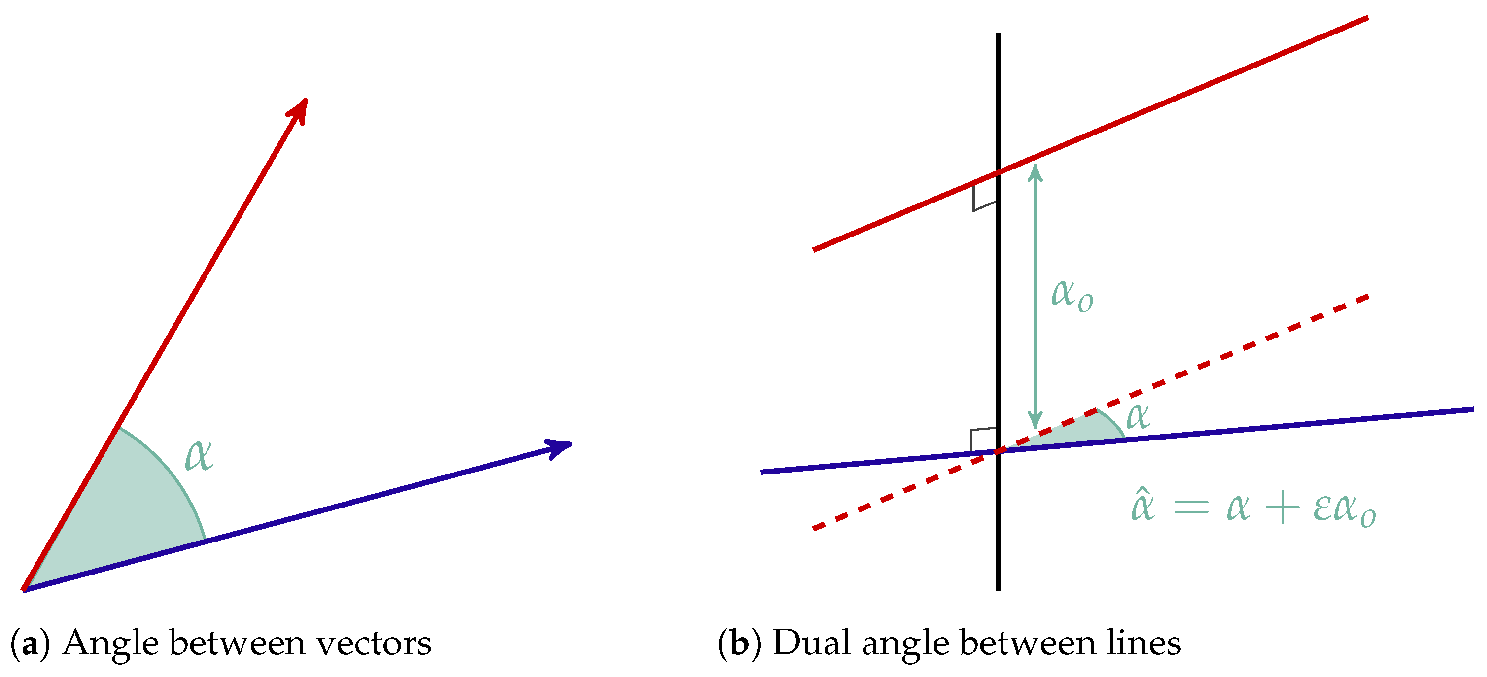
Figure 1. Geometric interpretation of angles and dual angles.
Machines 12 00402 g001
Figure 2. Illustration of a line vector by Plücker coordinates. p represents a point in the line, v gives the direction of the line and ( v ; p × v ) is the line in Plücker coordinates.
Machines 12 00402 g002
Figure 3. Dual rotation (rotation and translation) using the left operator dual quaternion.
Machines 12 00402 g003
Figure 4. General Twist Operation in a line. (a) Discontinuous screw motion consisting of rotation followed by translation. (b) Continuous screw motion using the concept of the screw pitch.
Machines 12 00402 g004
Figure 5. Applying the qt twist operation in a general line. The operated line v ^ is first rotated around v ^ r , then it is translated by t .
Machines 12 00402 g005
Figure 6. Timeline of kinematics-related works [1,2,16,17,19,21,22,23,24,35,38,39,40,41,42,43,44,45,46,47,48,49,50,51].
Machines 12 00402 g006
Figure 7. Timeline of control-related works [24,29,46,69,78,81,84,86,90,91,94,95,96,97,98,99,100].
Machines 12 00402 g007
Figure 8. Wordcloud with the keywords of the articles in this work.
Machines 12 00402 g008
Figure 9. Articles containing dual quaternions in their title from 1900 to 2023, according to Google Scholar.
Machines 12 00402 g009
Figure 10. Illustration of reference configuration and convenient fixed coordinate system.
Machines 12 00402 g010
Figure 11. Kinematic control of a omnidirectional robot going from ( 5 , 5 , π 2 ) to ( 0 , 0 , 0 ) . Adapted from [78].
Machines 12 00402 g011
Figure 12. Motion interpolation comparison between Euler angles and slerp. Adapted from [63]. (a) Linear interpolation of position vectors and Euler angles of coordinate systems A and B produces in-between poses with different orientations and positions. (b) Linear interpolation of position vectors and spherical linear interpolation (slerp) of coordinate systems A and B produces parallel yet displaced in-between poses.
Machines 12 00402 g012
Figure 13. Motion interpolation comparison between sclerp and C 1 interpolation of dual quaternions. Adapted from [63]. (a) Linear interpolation of dual quaternions (sclerp) representing coordinate systems A and B produces unambiguous in-between poses. (b) C 1 interpolation of dual quaternions: A smoother curve is achieved at key pose 2 while unambiguity is preserved.
Machines 12 00402 g013
Disclaimer/Publisher’s Note: The statements, opinions and data contained in all publications are solely those of the individual author(s) and contributor(s) and not of MDPI and/or the editor(s). MDPI and/or the editor(s) disclaim responsibility for any injury to people or property resulting from any ideas, methods, instructions or products referred to in the content.