Abstract
Strut-based or open lattice materials are a category of advanced materials used in medical and aerospace applications due to their properties, such as high strength-to-weight ratio and energy absorption capability. The most prominent method for the fabrication of lattice materials is the Laser-based Powder Bed Fusion (L-PBF) additive manufacturing (AM) process, due to its ability to produce parts of complex geometries. The current work presents an efficient meso-scale finite element (FE) modeling methodology of the L-PBF process demonstrated in the fabrication of body-centered cubic (BCC) lattice materials. The modeling efficiency is gained through an adaptive mesh refinement technique, which results in accurate and efficient prediction of the temperature field during the process evolution. To examine the efficiency of the modeling method, the computational time is compared with that of a conventional FE simulation, based on the element and birth technique. The temperature history difference between the two approaches is minor but the adaptive mesh modeling requires only a small portion of the simulation time of the conventional model. In addition, the computational results present a good correlation with the available experimental measurements for various process parameters validating the presented efficient method.
1. Introduction
Cellular materials and structures can be defined as an interconnected network of solid struts, plates, or shells, which form the edges or the faces of cells arranged together to fill the space [1,2]. These structures, which are also known as architected cellular materials or meta-materials, have found wide industrial use over the last two decades especially in energy absorption, aerospace, and biomedical applications [3,4,5]. The main types of cellular materials are engineering foams and lattice materials [6]. Lattice structures differ from foams by the regular repetitive structure of their unit cells [7]. Despite their resemblance with open-cell stochastic foams due to their significant periodic structure, lattice materials can achieve unique properties through the design of their unit cell and their precise manufacturing control. The most common topologies of lattice material unit cells are the strut-based topologies [6]. Metallic materials are usually used for the fabrication of strut-based lattice materials due to the provided design flexibility that allows them to tailor their density and properties [8]. For these reasons, these structures provide increasing opportunities for applications in advanced structural components and parts, where a high strength-to-weight ratio is desirable [9].
Additive manufacturing (AM) processes have been proven to be the most advantageous method for the production of lattice materials contrary to conventional manufacturing processes, such as investment casting or textile weaving [9]. In AM methods, parts are fabricated in a layer-by-layer manner based on the input digital model, thus, providing more design freedom to engineers and manufacturers contrary to subtractive and forming manufacturing techniques [10,11,12,13,14,15,16]. Among the various AM processes, the Laser-based Powder Bed Fusion (L-PBF) process is widely adopted in the industry and has reached a high level of maturity, with fabricated parts of excellent quality produced by various types of metal alloys [5,10]. The L-PBF process utilizes a high-power laser beam as a heat source to melt the powder layer based on a pattern defined by the induced digital model and when the processed layer is finished, the bed moves downward and the process is repeated on a layer-by-layer basis until the part construction is finished [5,14]. Due to typical track widths of 0.1–0.2 mm achieved with this method; very complex structures can be manufactured, making the L-PBF process the most prominent method for the fabrication of metallic lattice materials [5].
The modeling methods of the L-PBF process usually employ numerical simulation methods, with the finite element (FE) method being the most pronounced [17]. Besides the typical FE modeling procedures of geometry discretization and the subsequent load application, the simulation of the AM process requires extra stages that add complexity to the modeling, such as the modeling of material addition in a layer-wise fashion; the movement of boundary conditions due to laser scan strategies; material phase change, including material changes from powder to solid; and heat loses to powder bed [17,18]. These complexities have led researchers of AM simulation to focus on the phenomena of different spatial and temporal scales such as melt pools, multiple scanning tracks, single-layer simulations, layer-by-layer simulations, and part-scale simulations. Each scale is different in terms of sophistication and different considerations are needed to capture the phenomena of interest. In meso-scale models, the powder layer is assumed to be a continuum with averaged thermo-physical properties and the focus is laid upon the investigation and the prediction of temperature profiles in single or multiple layers, the subsequent distribution of residual stresses, and the estimation of melt pool dimensions [19,20,21]. Roberts et al. [22] developed a thermomechanical model with a Gaussian energy distribution for the laser beam heat source, temperature-dependent material properties, and the element birth and death technique to model layer addition and determined the temperature profiles and the residual stresses distribution in a small cuboid block; their results showcased an incremental increase in temperature between successive layers, although the complexity of the modeling approach made the simulation of only a few layers feasible. In the same manner, Li and Gu [23] utilized a moving laser heat source with Gaussian energy distribution to model the laser interaction with the powder bed and to examine the effect of laser power and scanning speed on the temperature distribution and melt pool geometric characteristics. Parry et al. [24] developed a thermomechanical model to investigate the evolution of residual stresses in a single layer with multiple scans L-PBF process for Ti-6Al-4V; they concluded that the stress distribution was dependent on the scan strategy with the stresses parallel to the scan vectors being higher than the transverse direction. The previous studies show that the modeling approaches that meticulously consider the thermal transfer phenomena are limited in L-PBF structures with small dimensions and cannot be applied in realistic-sized parts due to their enormous computational cost. Promising analytical models proposed in the literature [25,26,27] offered valuable insights. These solutions utilized a coupled thermomechanical modeling approach, incorporating factors such as moving heat sources and scan strategies for thermal effects [25,26,27], as well as employing Green’s functions to assess thermal stresses [25,26]. Notably, these analytical models demonstrated good agreement with experimental results, showcasing their predictive capability.
The previous modeling procedures were limited to the simulation of a single or a few layers due to their large computational cost. For this reason, the literature studies have also investigated the application of numerical schemes to increase the efficiency of L-PBF process simulation [28,29,30]. In particular, the implementation of adaptive mesh schemes in the L-PBF modeling and simulation is examined [28,29,30]. The mesh schemes were mainly applied for the simulation of small parts with simple prismatic geometry and highlighted the benefits in terms of minimizing the computational cost.
In the literature, the simulation efforts of the L-PBF process for the fabrication of lattice material structures are scarce. McMillan et al. [31] developed an efficient model based on the finite difference method for the prediction of temperature fields, based on a reduced-order one-dimensional transient tri-diagonal system of equations, that is suited to lattice geometries due to the slenderness of lattice strut elements. Downing et al. [32] developed a numerical model based on a reduced order numerical analysis to investigate the temperature field distribution of the cellular core during its fabrication in the L-PBF process; the input heat was applied once at the newly added lumped layer of cellular structure and the temperature fields showed that the lower layers of the struts developed higher temperatures than the upper layers of the cellular core. However, the previous works did not examine the effect of the main laser process parameters on the characteristics of lattice materials. In the work of Lampeas et al. [33], an element birth and death method was employed for layer addition and a moving heat source was applied in each layer for the simulation of L-PBF fabrication of a Ti-6Al-4V BCC unit cell; the computed strut diameter was used as an input to the homogenization of the unit cell for the investigation of BCC core mechanical properties, establishing a process parameters–structure–property relationship. Nevertheless, the efficiency of the modeling approach was not considered and the computational cost was very large.
In the present paper, a meso-scale modeling method is developed to improve the efficiency of the simulation of the L-PBF process. The modeling method is demonstrated in the simulation of the fabrication of open lattice materials and utilizes an adaptive mesh refinement approach, which results in a significant reduction in the computational cost. The introduction of an adaptive mesh scheme for simulating L-PBF fabrication of lattice materials marks a novel approach in the relevant literature. The results of the novel adaptive mesh refinement technique are compared with those of a more conventional modeling method, based on the element birth and death technique, to investigate their differences in accuracy and computational cost. Moreover, the simulation results are compared with the experimental measurements for various process parameters from the available literature to validate the current modeling method.
2. Materials and Methods
2.1. Lattice Materials Used for the Demonstration of the Modeling Methodology
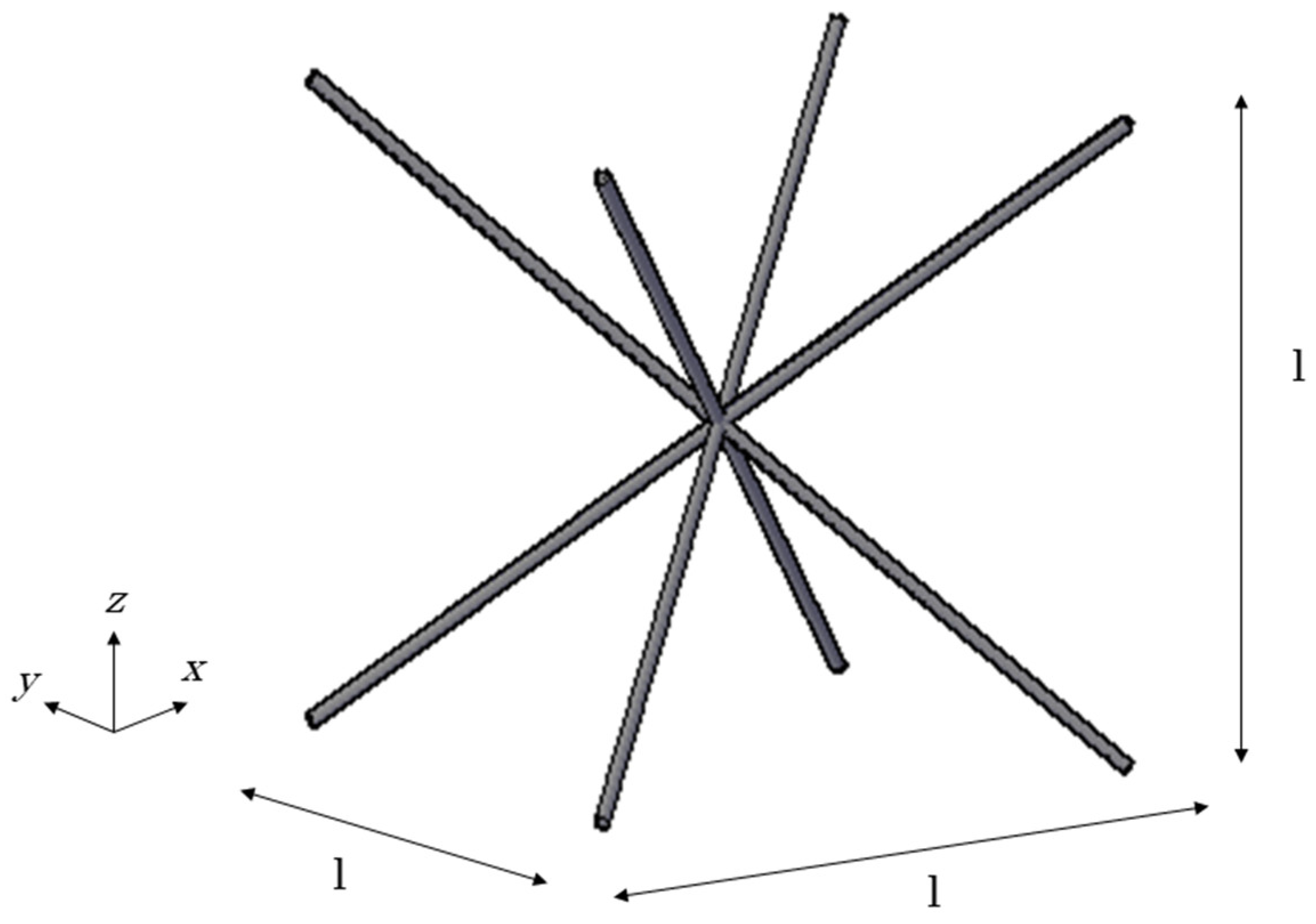
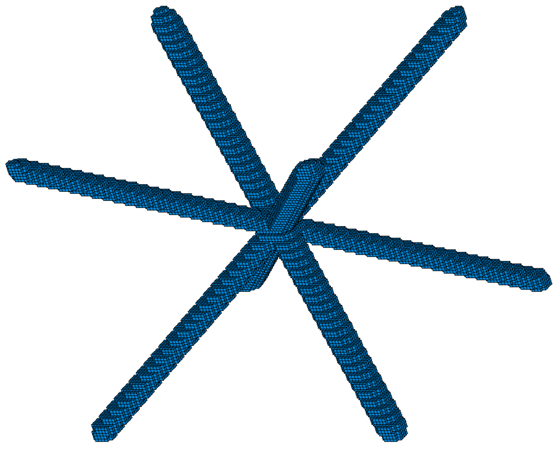
The presented meso-scale modeling method of the L-PBF process is applied for the simulation of the fabrication of lattice materials. Specifically, it is demonstrated for the L-PBF fabrication of a lattice material unit cell with a body-centered cubic (BCC) topology, presented in Figure 1. The unit cell consists of four micro-struts crossing each other at their middle span. The configuration of the BCC unit cell is typical of strut-based lattice structures. The size of the BCC unit cell is 2.5 mm and it is fabricated by Ti-6Al-4V on a steel substrate.
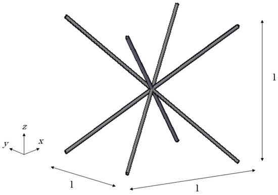
Figure 1.
Body-centered cubic (BCC) unit cell.
The simulation of the investigated lattice unit cell is performed with the L-PBF process parameters used in the work of Mullen et al. [34]. The lattice unit cell is built by laser heating the successive layers at the points that represent the centers of each strut cross sections. The laser system utilized a Yb (ytterbium) fiber laser with a power ranging from 80 to 200 W and operated at an operational wavelength of 1.06 μm. It featured a focused laser spot with a diameter of 100 μm, characterized by a uniform intensity distribution across its entire beam spot. For the creation of the lattice structure, the laser beam irradiates a spot on the powder material for a specific time period, varying from 500 to 1000 μs at a scanning speed of 1 mm/s. The process parameters of the experimental study considered in the present work are presented concisely in Table 1.

Table 1.
L-PBF process parameters applied in the fabrication of a BCC lattice material unit cell [34].
2.2. Modeling of the Heat Transfer Phenomena Occurred during the L-PBF Process
During the evolution of the L-PBF process, the heat energy is introduced to the processed powder layer through the laser beam radiation at the powder surface. Heat transfer takes place mainly in three ways, i.e., conduction, convection, and radiation, in the processed material. The equilibrium of energy is expressed as [33], as follows:
where , , , and are the laser beam heat input, the conduction, the convection, and the radiation losses, respectively, while is the energy related to phase transformations. Heat conduction for temperature-dependent conductivity can be expressed using the Fourier’s law as [30], as follows:
where is the temperature-dependent thermal conductivity, is the temperature of the part, is the rate at which heat energy is supplied to the system, is the density of the material, is the specific heat capacity, and is time. In the present simulation, the heat of the laser beam is modelled as a heat flux, while radiation effects are omitted, since they are considered minor, while heat losses by convection only are considered.
2.3. Temperature-Dependent Material Properties
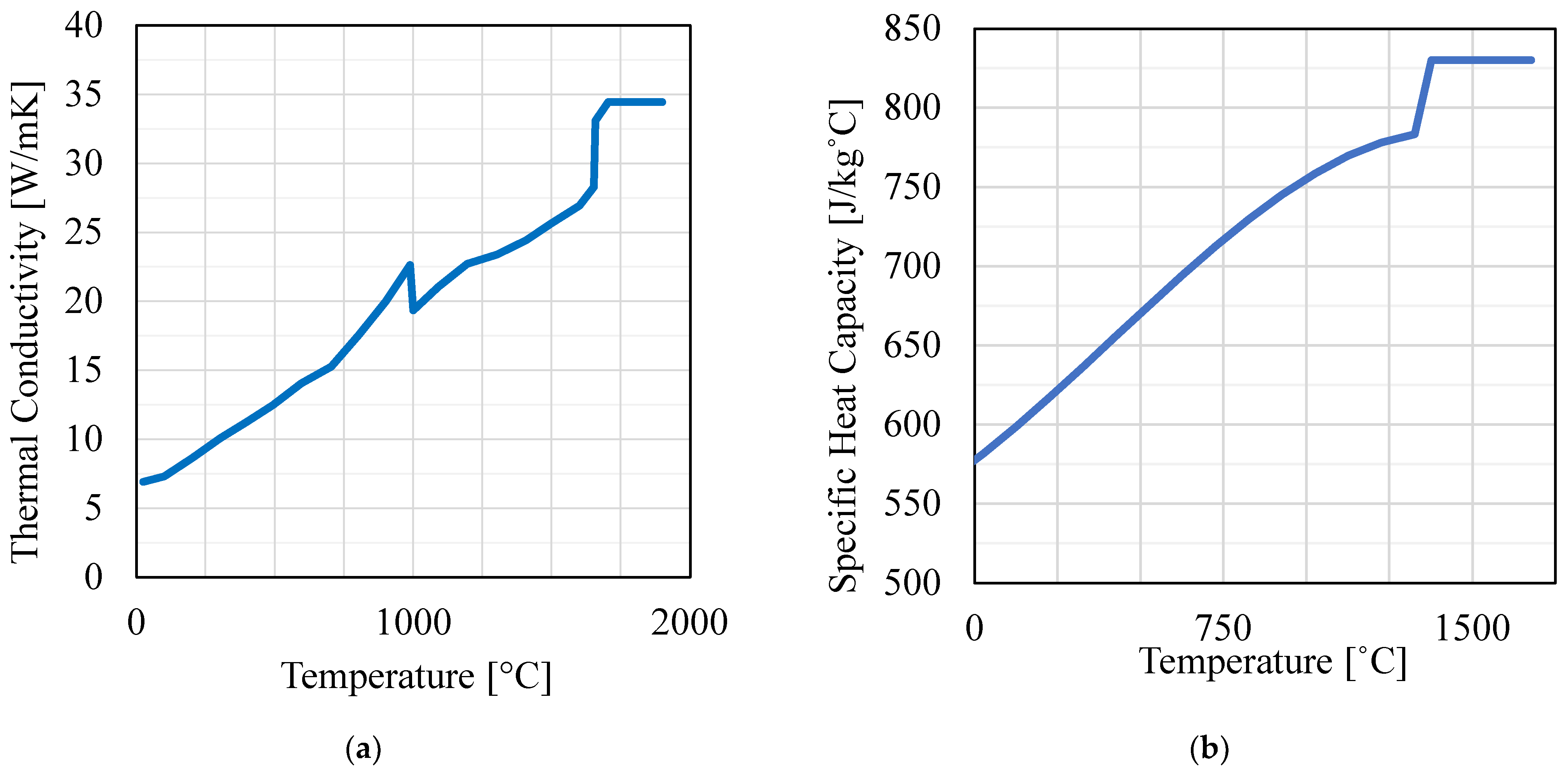
In the meso-scale modeling of the L-PBF process, the powder bed is considered as a continuum medium. During the L-PBF process, the processed powder bed of metal alloy experiences a large range of temperatures and goes through powder to the solid state. The introduction of temperature-dependent material properties in the analysis is crucial for achieving accurate simulations results. The temperature-dependent material properties considered in the present work are presented in the Figure 2a,b [35].
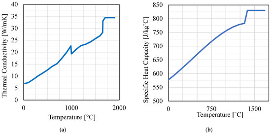
Figure 2.
Temperature dependent material properties used in the present analysis: (a) thermal conductivity and (b) specific heat capacity [32].
The thermal conductivity of the powder material is considered based on powder-solid relationships developed by Sih et al. [34], assuming that the particles are spheres and there is no flattening of contact surfaces. The effective thermal conductivity kp of the metallic powder consisting of spherical particles is calculated as follows:
where kf is the thermal conductivity of the argon gas surrounding the particles, φ is the porosity of the powder bed, ks is the conductivity of the solid, and kr is heat transfer attributed to the radiation amongst the individual powder particles.
where Dp is the average diameter of the powder particles and is the Stefan-Boltzmann constant (σΒ = 5.67 × 10⁻⁸ W/m2K4). The specific heat capacity is assumed to be the same for both bulk and powder material. The density of the powder and solid material are 2.64 and 4.4 g/cm3, respectively, for the Ti6Al4V metal alloy and are considered independent of temperature. The substrate material is steel, for which temperature-dependent material properties (thermal conductivity) are also utilized. The considered material properties of the Ti-6Al-4V are presented concisely in the Table 2.
Table 2.
Material properties of Ti-6Al-4V were considered in the analysis [34,35].
2.4. Efficient Modeling Procedure and Adaptive Mesh Refinement Technique
Adaptive mesh refinement is one of the main numerical techniques for the minimization of the computational cost in FE modeling and simulation. This technique is explored in an innovative way in the currently developed modeling methodology, aiming to increase the efficiency of the meso-scale FE analysis of the L-PBF process.
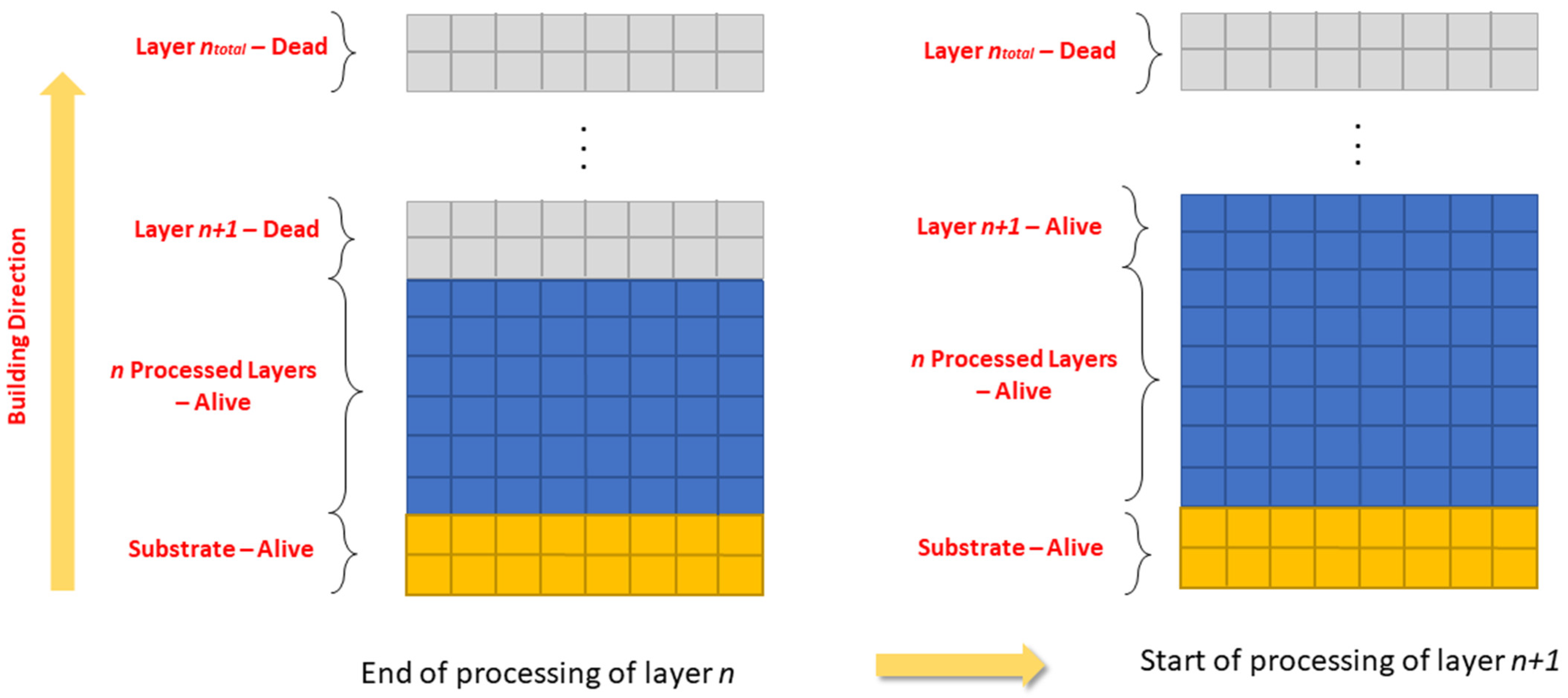
The common mesh strategy technique of the conventional FE modeling of the L-PBF process utilizes a cuboid mesh discretization of the powder bed and the region that contains the AM part. The ‘element birth and death’ technique is usually employed in order to keep the system stiffness matrix small at the beginning of the process, increasing it step-wise, together with the successive addition of the layers. Practically, this means that all the elements of the cuboid discretized part are initially in ‘dead’ status, which means that they do not contribute to the stiffness matrices of the elements. As the process evolves and layers are added, the corresponding elements are turned to status ‘alive’, meaning that the elements that discretize the respective layers are activated and begin to contribute to the stiffness matrix. The schematic description of the ‘element birth and death’ technique is presented in Figure 3. The main characteristic of this approach is that the meshing of the processed region remains the same throughout the simulation of the L-PBF process. However, this leads to an increasing computational cost, which continuously increases and becomes extremely large toward the last stages of the process simulation.
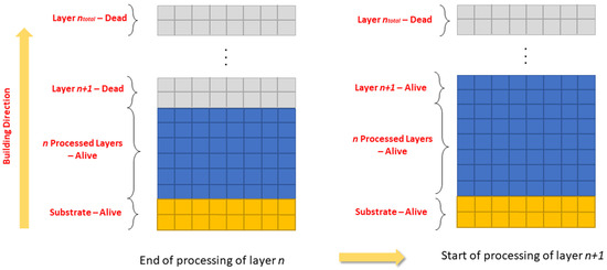
Figure 3.
Schematic description of the element ‘birth and death’ technique.
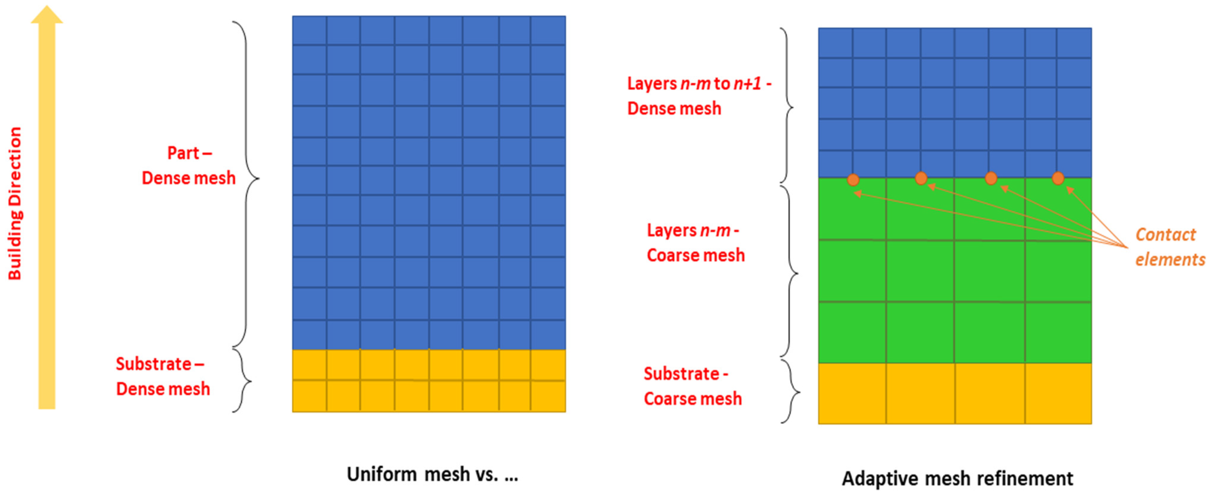
Aiming to overcome this drawback, an adaptive mesh refinement technique is explored in the meso-scale L-PBF simulation. The approach is based on creating a dense mesh discretization for the layer under processing in the corresponding time step. The same dense mesh discretization is also applied to a small number of layers underneath the processed layer, as these layers have high-temperature gradients as well. On the contrary, a coarse mesh discretization is applied in the layers that have been already processed and are not located close to the processed layer as they do not play an important role anymore. The high-density mesh used for the discretization of layers that are processed in a time step basically aims to capture the nonlinear phenomena around the melt pool and the heat-affected zone (HAZ), while the nonlinear thermal phenomena do not significantly affect the temperature gradients and distribution of the layers that are in a certain distance from the processed layers. Contrary to the conventional meshing strategy, in the present adaptive mesh refinement technique, the processed region is not meshed with the same density as during the analysis. Every discretized layer is added in the model as the process evolves at an element size that is initially small, based on the discretization needed to model the laser heat source spot, while the mesh is coarsened after the heat source moves away from it. With this approach, the total number of elements is highly reduced compared to a model with a uniform dense mesh. The schematic description of the adaptive mesh refinement technique is presented in the Figure 4.

Figure 4.
Schematic description of the adaptive mesh scheme and its comparison with the uniform mesh approach.
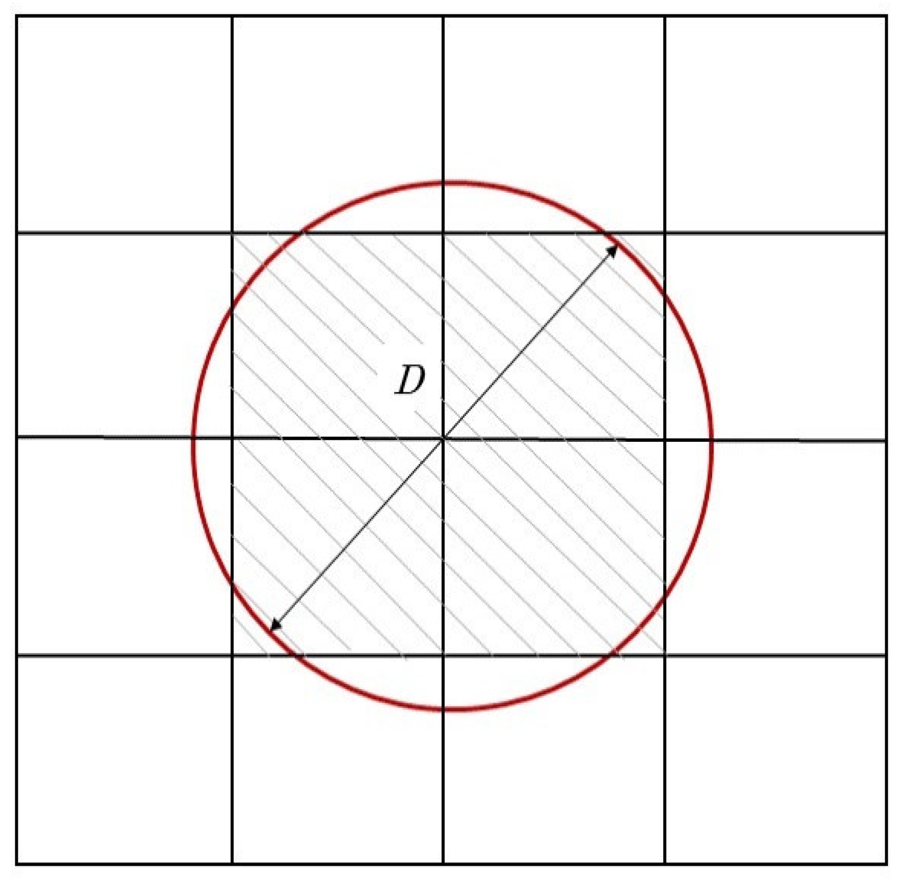
The laser beam is modelled as heat flux introduced in the material as a uniformly distributed heat input on the surface elements that their entire face is covered by the laser beam spot. The magnitude of the heat flux is derived by the following equation:
where is the laser heat power, is the laser beam radius, and is the laser energy absorptance of processed material. Due to the cuboid FE discretization of the powder bed, the circular laser spot cannot fully cover the surface of each element. Therefore, it is assumed that an element receives heat if more than half of its surface is covered by the laser spot, as it is depicted in Figure 5. In this case, the surface nodes of the element are considered to receive heat.
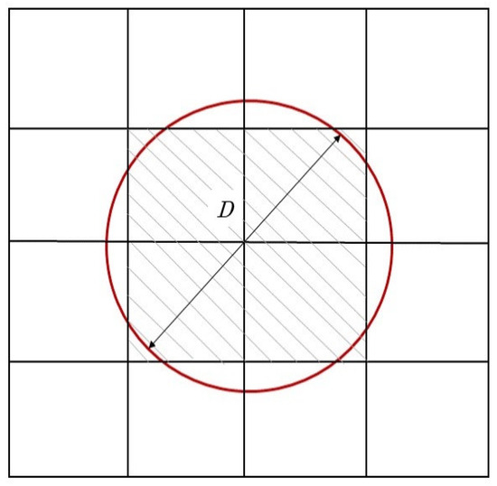
Figure 5.
Application of the constant heat flux on the elements covered by the laser spot diameter.
The laser energy absorptance of a material depends on several factors, such as the nature of the surface, the level of oxidation, the wavelength of the laser, and the surface temperature [36]. Here, the value of absorptance is considered to be 0.3, equal to the absorptance value of the bulk pure titanium material at the Nd:YAG wavelength, an approach also followed in the relative literature [22].
The L-PBF fabrication of the BCC unit cell is modeled with both ‘element birth and death’ and adaptive mesh techniques. The results of the ‘element birth and death’ model for the prediction of the temperature fields serve as a reference for comparison with the results of the efficient model. Also, the computational times for these approaches are compared to determine the efficiency of the adaptive mesh refinement method. Moreover, in order to validate the present thermal modeling methodology, the strut dimensions resulting from the selected process parameters are compared with available experimental measurements found in the literature work [31].
2.5. FE Modeling Procedures
The procedures for the development of the reference FE model based on the ‘element birth and death’ approach and the efficient models based on the adaptive mesh refinement approach are presented in this section. The models are developed in ANSYS APDL 2020R2 commercial FE software [37]. Eight-node hexahedral solid elements (SOLID70) are used for the discretization of the unit cell (part) and the substrate. This element type has eight nodes with one degree of freedom at each node, the nodal temperature. Node-to-surface contact element pairs (CONTA175-TARGE170) are used for the joining of the two mesh schemes of the part and the substrate. These contact element pairs are utilized for the modeling of the interface between the building part and the substrate to ensure temperature continuity and the proper heat transfer conditions.
The element size of the reference FE model is determined based on a mesh convergence study performed for different element sizes. In the first FE model, the element size is set to 50 μm; thus, two elements per laser beam diameter are defined. This FE model consisted of 145,656 nodes and 137,500 elements and has been proven rather rough for the specific application. Convergence is assessed by examining the temperature fields in the heat-affected zone and the resulting strut diameter, ensuring that differences between consecutive mesh resolutions are minimized to achieve convergence. In the second FE model, the element size is 25 μm, corresponding to four elements per laser beam diameter. The resulting FE model consisted of 1,081,306 nodes and 1,050,000 elements. This FE model requires reasonable solution time (of the order of some hours using an 8-core workstation), while it provides reasonably accurate results. Particularly, comparisons with experimental measurements of strut diameters validated the accuracy of the selected element size, corroborating the fidelity of the numerical predictions. Given the intricacies of the L-PBF process, finer mesh resolutions are examined to capture nuances such as thermal gradients and material deposition more accurately. In the third FE model, the element size is 12.5 μm, (eight elements per laser beam diameter). This FE model consists of 8,522,606 nodes and 8,8400,400 elements. The size of the third FE model has the consequence of prohibitively long computational times, without significantly improving results accuracy. Specifically, the difference in the average strut diameters calculated by the second and third models has been less than 10 μm. Therefore, an element size of 25 μm is considered converged and selected for the current simulation of the L-PBF fabrication of the BCC unit cell. Table 3 presents the concise mesh characteristics of the models developed during the mesh convergence analysis.
Table 3.
Characteristics of the ‘element death and birth’ FE models developed for the mesh convergence study.
Three parametric variations in the adaptive mesh refinement modeling approach are tested, based on the number of dense layers used to simulate the nonlinear phenomena around the melt pool. This parametric analysis is performed to determine the necessary number of dense layers above the coarse layers for an accurate analysis. The three model variations contained 3, 4, and 5 dense meshed layers underneath the processed layer. These models are referred to as Fast Model-3, Fast Model-4, and Fast Model-5, respectively. As already mentioned, in the FE model based on the adaptive mesh refinement approach the geometry is not defined from the beginning of the simulation; when the processing of a layer finishes, a new layer is added to the model. The size of the elements of the fine mesh and coarse mesh are 0.25 mm and 0.50 mm, respectively. This strategy is based on the fact that the top layers are those influenced the most by the heat input by the beam, characterized by a high degree of non-linearity, while the effect of the beam decreases as we move toward the bottom layer and the heat transfer phenomena become more linear. The melt pool is also limited to a few layers below the top layer. Since the fine and the coarse mesh have different densities, they should be joined at their interface. Eight-node hexahedral solid elements (SOLID70) are used for the discretization of the unit cell and the substrate. The joining of the two meshes is performed using contact elements. Node-to-surface contact pairs, consisting of CONTACT175 and TARGET170 elements, are used to join the two meshes. With the use of the contact pair, each node of the fine mesh is now connected with the element of the coarse mesh located below. An important parameter in a contact pair is the conductivity of the contact. In our case, the contact conductivity was selected to be equal to the conductivity of the powder. This approach is followed because most of the contact regions are in a powder state. In addition, testing was conducted using the conductivity of the solid material as the conductivity of the contact and no differences were observed in the results. It should be stated, however, that generally increased attention should be given to the contact conductivity considering the specific model geometry and the nature of the contact under investigation. As the process evolves and the subsequent layers are added to the part, the new layers enter the model with a high-density mesh and the previous mesh for the bottom layers is updated to the low density.
The mesh characteristics of these models at the last step of analysis are presented in Table 4. The size of the models is dramatically decreased compared to the reference FE model.
Table 4.
Mesh characteristics of the efficient FE models at the last step of analysis.
Since the presented adaptive mesh refinement procedure is not a built-in feature of ANSYS APDL 2020R2 software, a special code is developed to guide the procedure. The code is used to create the mesh nodes in their respective positions and then to create the elements from those nodes. In order to transfer the results from one step of the analysis and use them as initial conditions for the next step, each node must maintain the same number throughout the process. The numbering technique ensures that each node retains the same identifier throughout the adaptive mesh refinement process, regardless of its location in a dense or coarse mesh region. That way, continuity and consistency in node numbering are maintained, facilitating the accurate transfer of analysis results and application of initial conditions in subsequent analysis steps.
At the beginning of the processing of a new layer, powder material properties are attributed to all elements of this layer. During the evolution of the L-PBF process, when the elements reach the melting temperature of the processed alloy, they solidify and solid material properties are assigned. In all models, the convection coefficient is considered equal to 20 W/m2⋅°C, a value also considered in the relative literature [30].
3. Results
3.1. Thermal Analysis Results
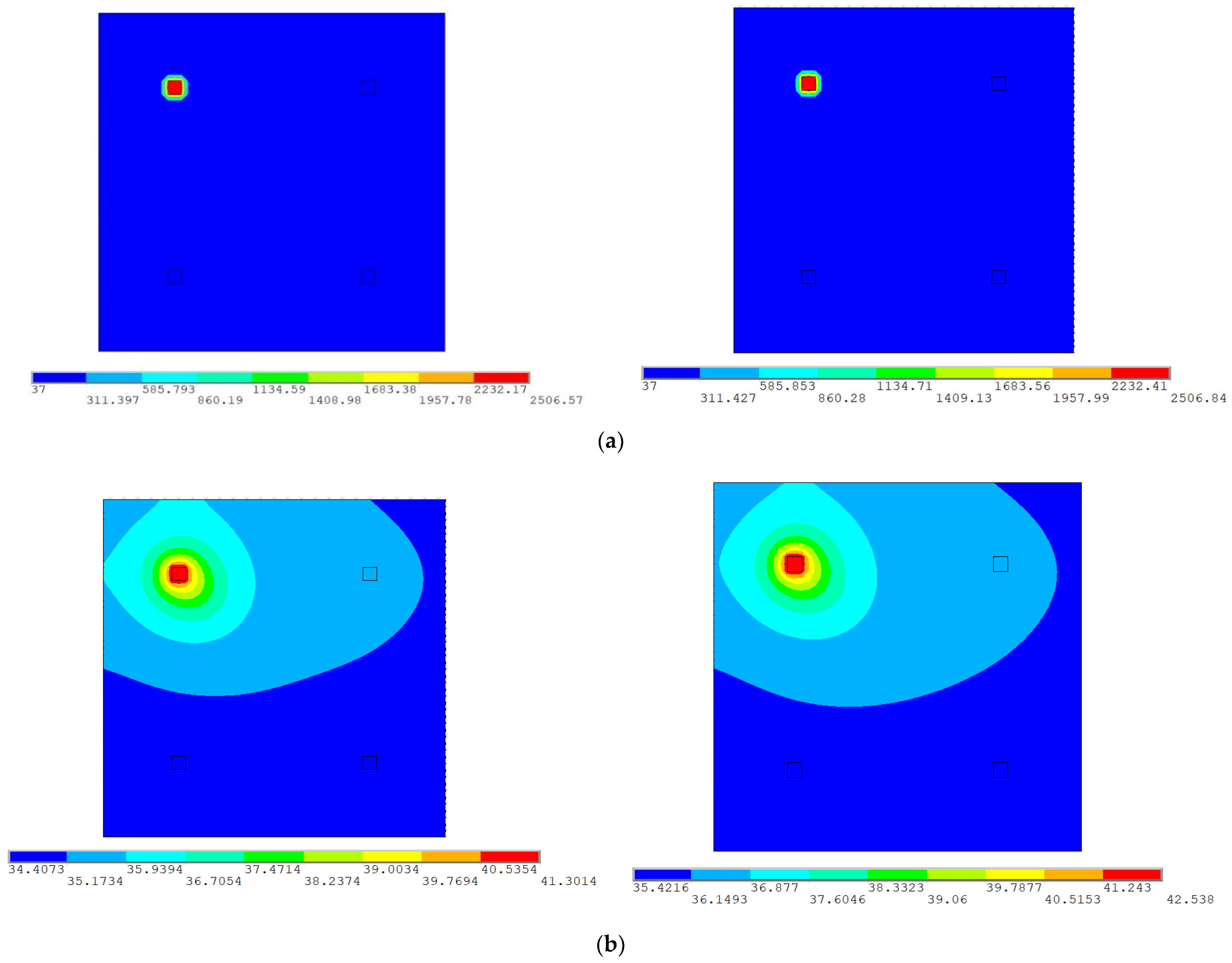
The temperature distribution on a laser-scanned point at a representative layer of the BCC unit cell is presented for reference and the fast FE models. The comparison between the contour plots of the temperature distribution at a laser spot point of the 40th layer as derived from the reference ‘element birth and death’ and the fast FE model with 5-dense layers are presented in Figure 6a,b. The temperature fields are presented for the heating and cooling load step of the analysis. The heating cycle is the time for the laser irradiation on the spot and the cooling cycle is the time the laser beam moves to the next spot during which there is no irradiation on the surface of the powder layer. The differences in presented temperature fields are minor as both the shape of HAZ and the temperature values are almost identical. This denotes a qualitative good correlation between the conventional and the novel modeling approach.
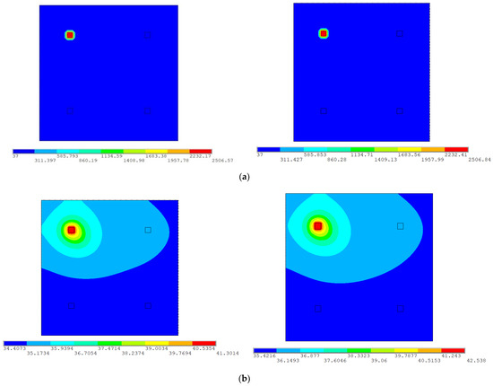
Figure 6.
Contour plots of the predicted temperature fields as derived from the reference FE model (left column) and the fast model with 5 dense meshed layers (right column) in the 40th layer at (a) the heating load step and (b) the cooling load step of fourth laser spot of the layer.
To obtain a quantitative insight into the temperature distribution differences between the two modeling approaches, the temperature variation at the surface and depth are examined for reference and the fast models.
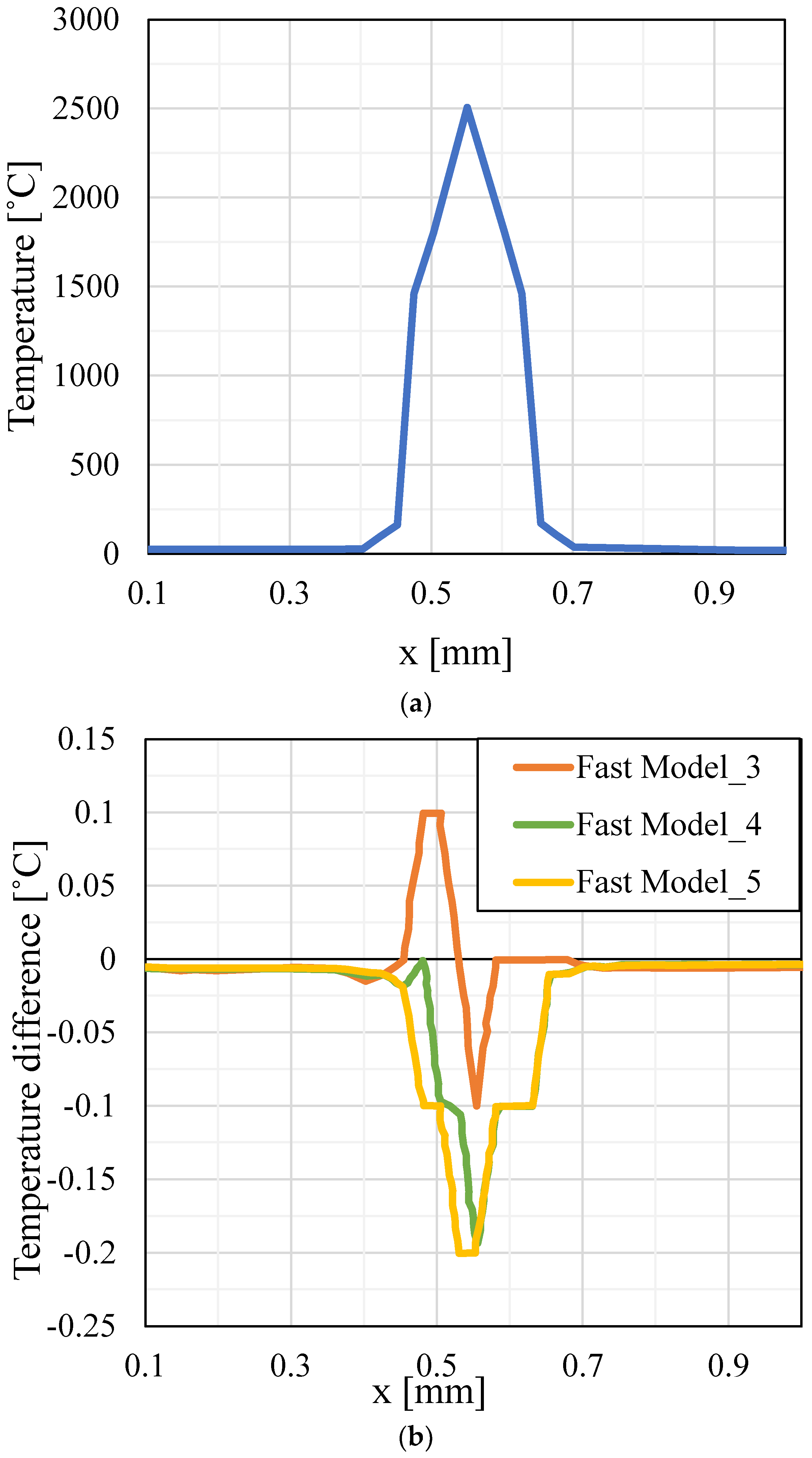
The surface temperature distribution along the line that passes through the center of the melt pool of the first laser exposure point at the 40th layer during the heating and cooling load step is examined. The comparison between the results of the reference and the fast FE models during the heating and cooling load step is presented in the diagrams of Figure 7 and Figure 8, respectively. Figure 7a and Figure 8a present the temperature variation in the reference FE model and Figure 7b and Figure 8b present the temperature differences between the reference and the fast FE models. The temperature difference becomes maximum at the center of the melt pool and it decreases away from it for both the heating and cooling steps. At the heating step, the temperature differences between the reference FE model and fast FE models are minor, showing that the temperature fields on the surface are almost identical. However, during the cooldown cycle, the differences between the models become higher. The fast model with three dense layers presents a 6% difference from the reference model at the temperature peak, while the fast models of four and five dense layers have a difference of about 1%. This feature can be attributed to the small number of elements used in the fast model for the three dense layers for the modeling of rapid heat transfer between the upper and downward layers. It is shown also that four or five dense layers are sufficient to model the heat transfer to the already processed layers.
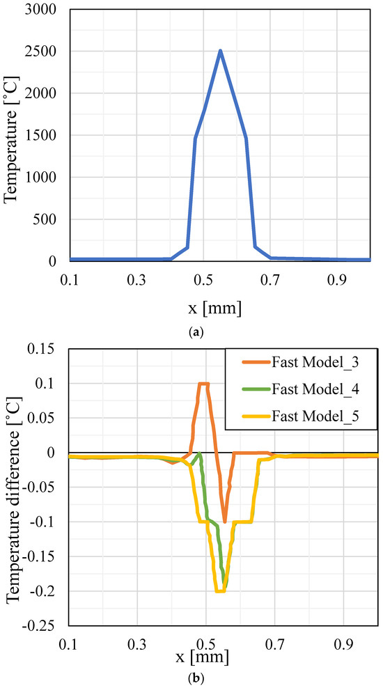
Figure 7.
Thermal results at the surface of the first laser spot of the 40th layer at the heating step: (a) temperature distribution of the reference FE model and (b) temperature differences between the reference and the fast models.
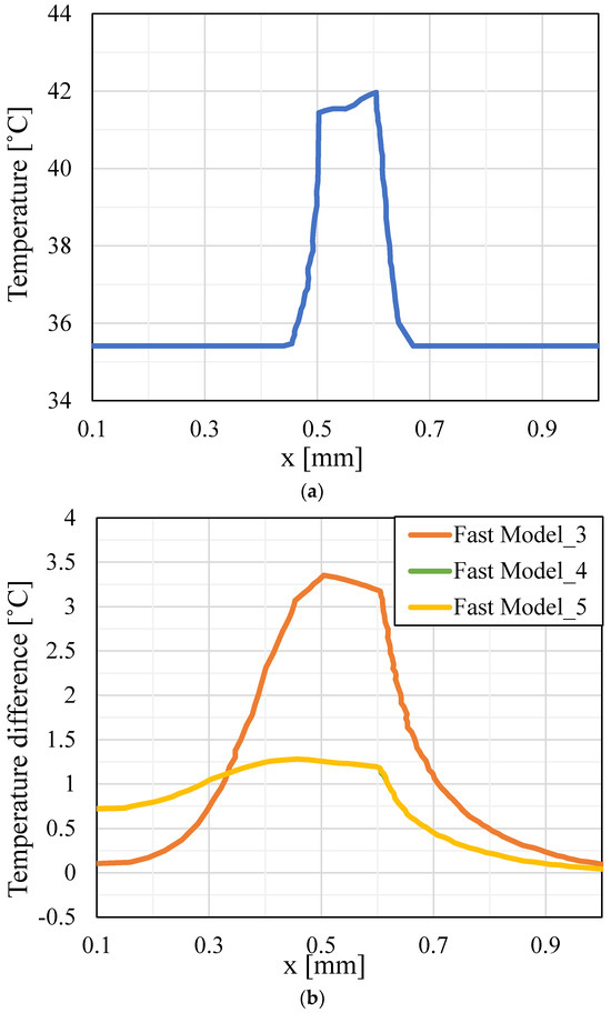
Figure 8.
Thermal results at the surface of the first laser spot of the 40th layer at the cooling step: (a) temperature distribution of the reference FE model and (b) temperature differences between the reference and the fast models.
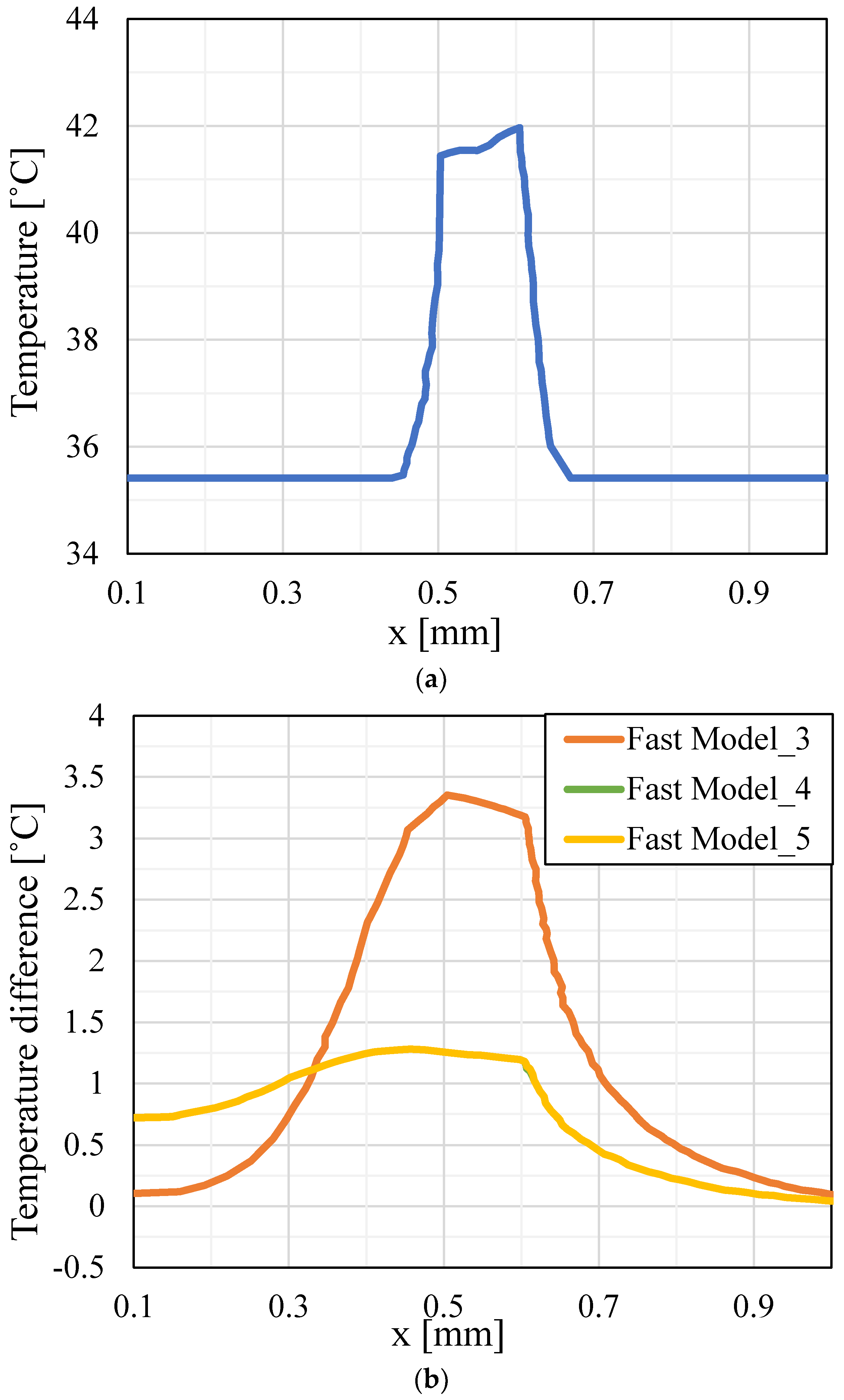
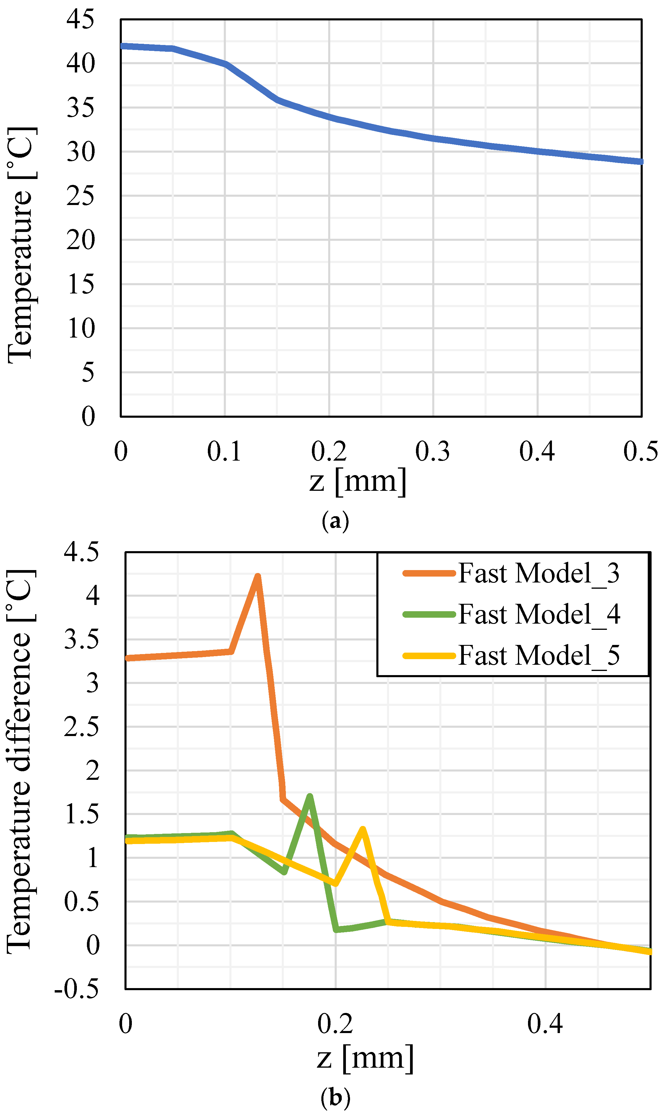
The temperature distribution along the depth of the melt pool is further examined at the same irradiation spot. Figure 9 and Figure 10 present the temperature distribution and temperature differences along the depth of the melt pool for thermal and cooldown cycles, respectively. Temperature distribution becomes maximal at the surface of the processed layer for both the thermal and cooldown cycles. At the end of the cooldown cycle, the temperature distribution decreases and the layer-wise temperature field becomes more homogeneous. The higher temperature differences are presented near the surface of the processed layers (z = 0.15) and they are minimized toward the depth of the part. At the thermal cycle, the temperature differences are very small for all models. However, at the cooldown cycle, the difference between the fast model with three dense layers has a maximum difference of 10% at the peak of the temperature distribution, while the maximum difference in the models with four and five dense layers is 2.5–3%. The same trending of temperature differences is observed at the cooldown temperature distribution at the surface of the processed layer. This denotes that although the adaptive mesh model with three dense layers can provide useful insight into the thermal fields, its accuracy is limited, especially in the cooldown cycle. Thus, adaptive discretization with four or five dense layers is preferable.
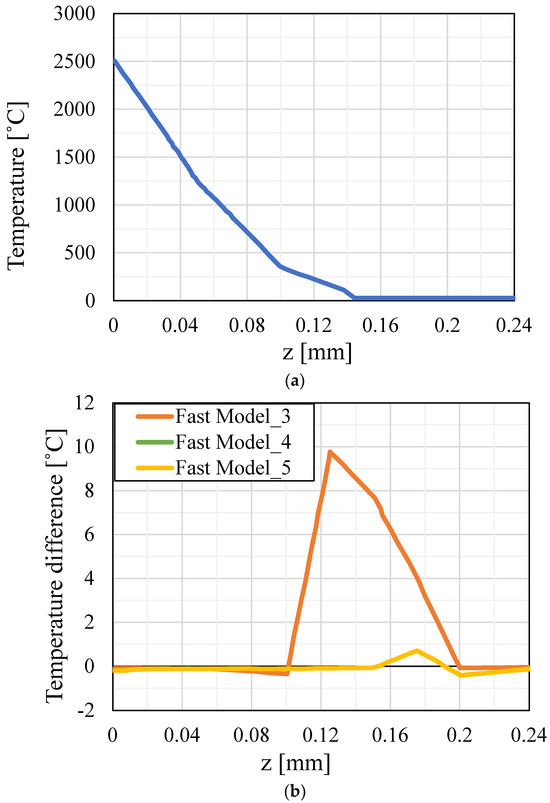
Figure 9.
Thermal results along the depth of the first laser spot of the 40th layer at the end of the thermal cycle: (a) temperature distribution of the reference FE model and (b) temperature differences between the reference and the fast models.

Figure 10.
Thermal results along the depth of the first laser spot of the 40th layer at the end of the cooldown cycle: (a) temperature distribution of the reference FE model and (b) temperature differences between the reference and the fast models.
Overall, the numerical thermal results verify the ability of adaptive mesh modeling methodology to reproduce results of the same accuracy as the conventional ‘element birth and death’ technique with the suitable selection of dense layers.
3.2. Computational Time
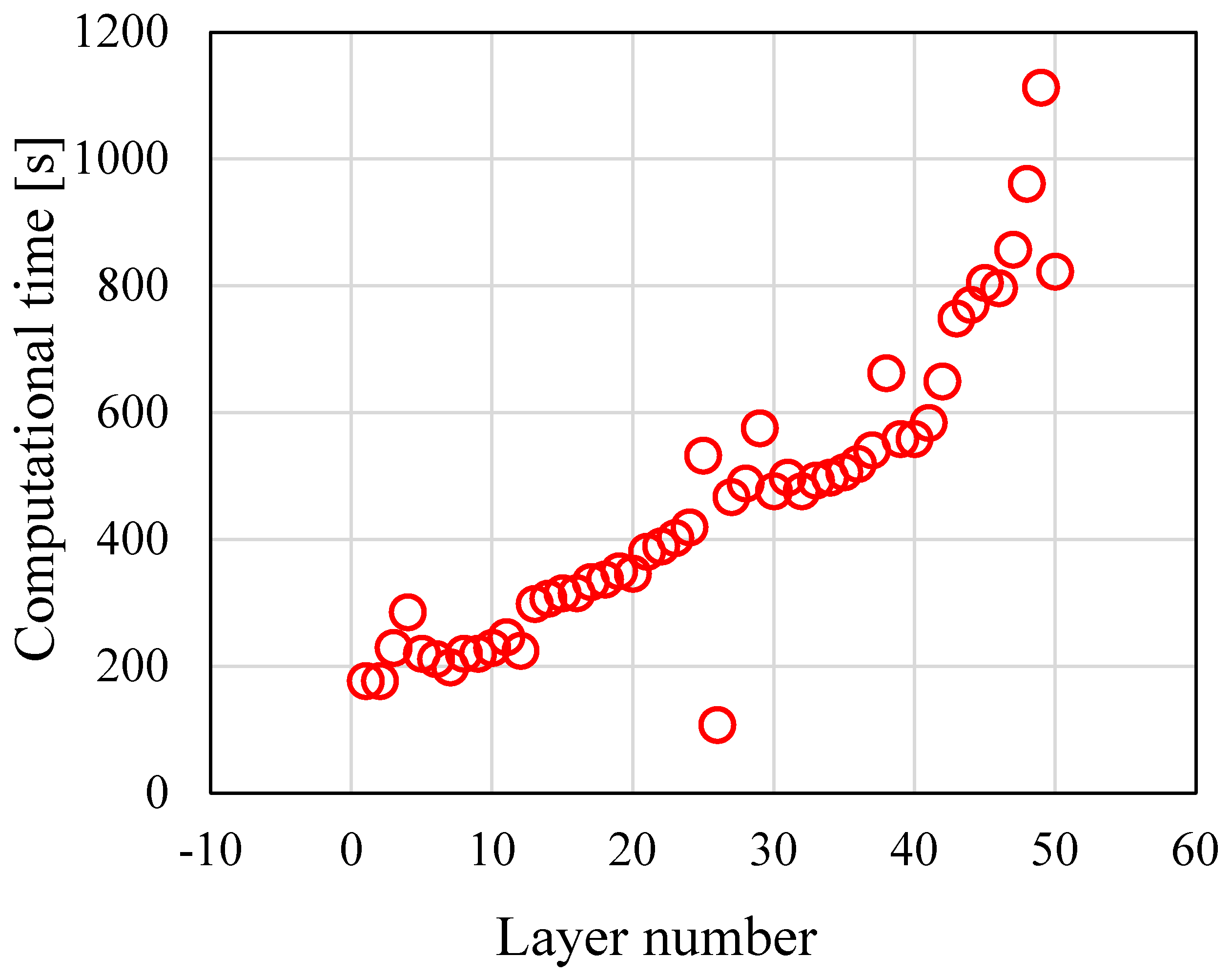
The computational time of the examined models is presented in this section. The presented simulations have been performed on a computer system of 8-Core 3.70 GHz CPU with 16 GB RAM. Firstly, the computational time of each layer for the reference FE model is presented in Figure 11. The computational time increases steadily as more layers are added. The only exception is the middle layer in which the computational time is significantly less than the time required for the other layers. This is ascribed to the fact that this layer is irradiated by the beam at a single point as we have reached the junction of the beams. Therefore, this layer is simulated in two stages (heating and coating) and the computational time is drastically reduced.
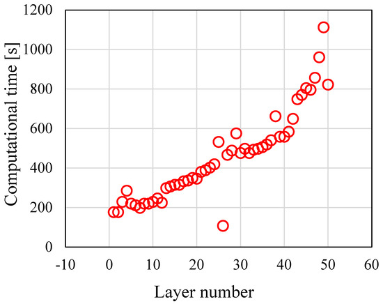
Figure 11.
Computational time per layer of the reference FE model.
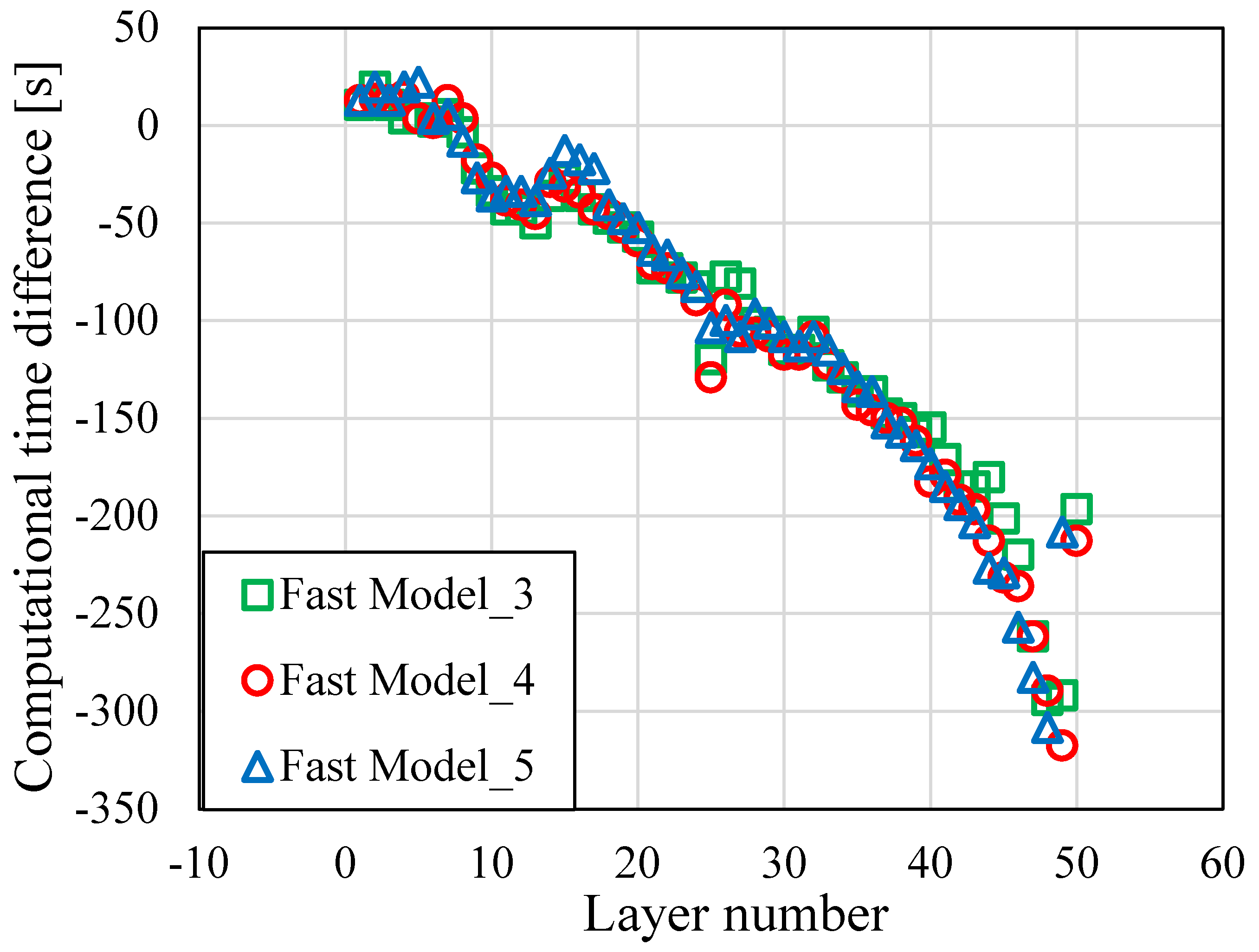
The computational time difference per layer between the reference model and the three fast models is shown in Figure 12. A radical reduction in computational time is achieved as the number of layers increases and densely discretized lower layers are replaced by coarsely discretized layers. More specifically, it can be observed that for all processing after the 10th layer, the computation time per layer is reduced by about 50% or more. The reduction is almost identical between the three models. Thus, it can be concluded that small changes in the number of densely discretized layers do not have significant effects on computational time.

Figure 12.
Computational time differences between the fast models and the reference model.
A comparison of total computational time between the reference and the fast FE models is presented in Figure 13. It can be observed that the total computational time of the fast models can save up to 70% of the computational time of the reference FE model. The differences between the computational times of the fast models do not surpass 8%. As expected, the model with the five fine layers requires the longest computational time. The model with the three fine layers does not require the shortest computational time. On the contrary, this is conducted by the model with the four fine layers. However, this can be attributed to differences in the number of iterations the solver needed for convergence.
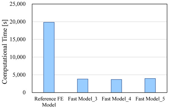
Figure 13.
Total computational time of the examined models.
3.3. Validation of the Modeling Method
In this section, a comparison between experimental measurements and numerical results of the ‘element birth and death’ model is presented. The final shape of the unit cell struts is defined by the topology of elements that have exceeded the melting temperature of Ti-6Al-4V alloy (1660 °C) at any stage of the manufacturing process simulation. The predicted final shape of the BCC unit cell is presented in Figure 14.
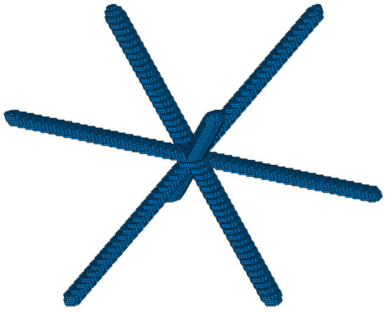
Figure 14.
Numerically predicted final shape of the BCC unit cell as assessed by thermal simulation results of reference FE model.
The numerical simulation results are compared to respective experimental measurements [28] for validation purposes. The diameter of the struts of the BCC unit cell structure predicted by the numerical simulations and the experimentally measured strut diameters of the Ti-6Al-4V are compared. As can be observed in Figure 14, the struts cross-section is neither perfectly circular nor perfectly constant along their length. Therefore, considering that the targeted strut cross-section is circular, five different circle diameters were used along the strut length to calculate the average diameter value. A comparison between the numerically determined and experimentally measured struts of the BCC unit cell is presented in Table 5. The mean values of the experimental strut diameter were considered for comparison with the experimental results. The error is 6.78%, which denotes the accuracy of the reference FE model.
Table 5.
Comparison between the mean values of experimentally measured and numerically determined strut diameters.
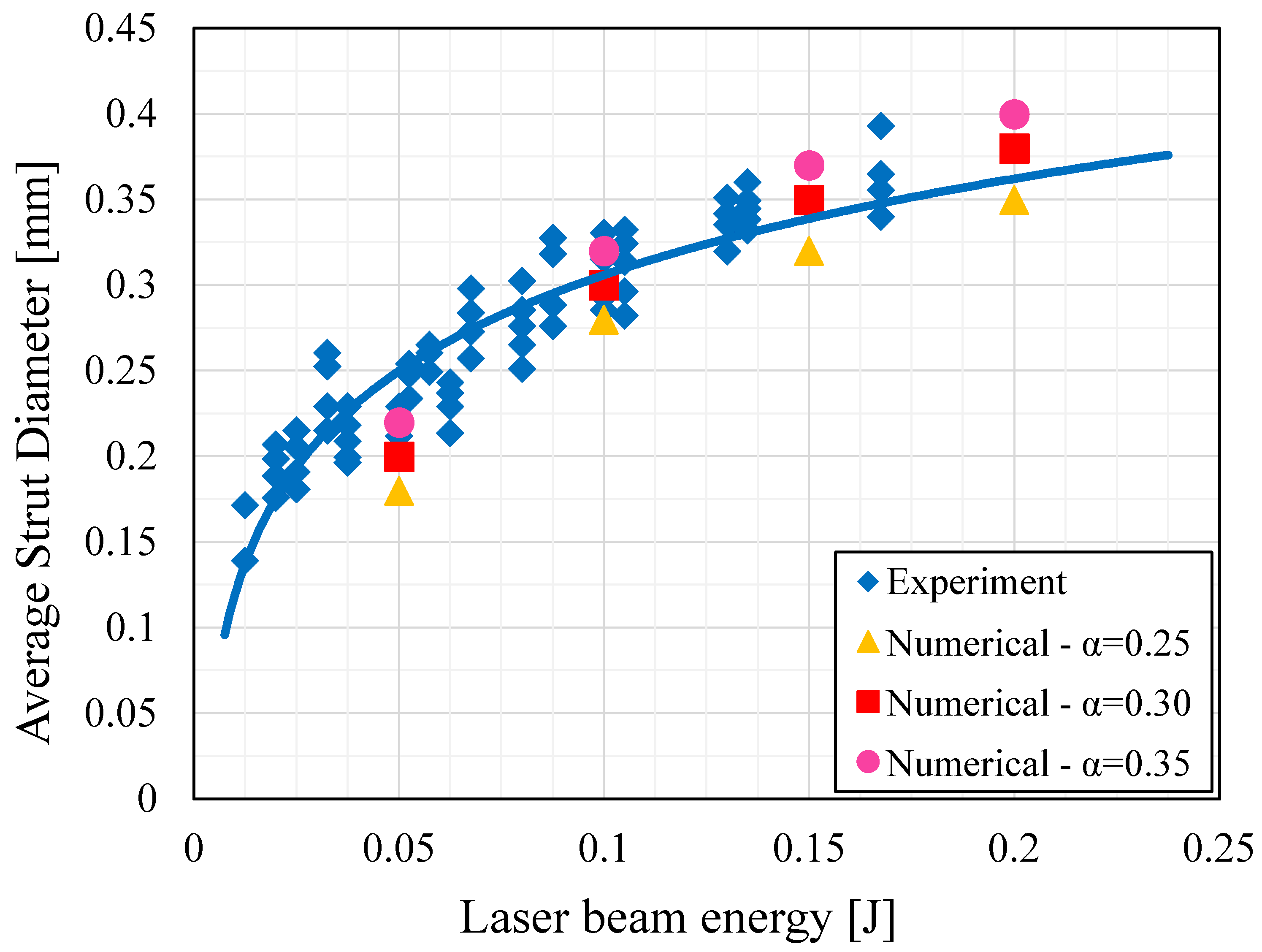
The simulation of the L-PBF for the fabrication of the BCC unit cell is extended for different laser beam energies and different laser power exposure times. The simulations are performed for different values of the absorptivity ratio (α), 0.25, 0.3, and 0.35, to check the sensitivity of this parameter. The correlation between the experimental and predicted strut diameters for the examined set of process parameters is presented in the diagram of Figure 15. The comparison of numerical results to the respective experimental measurements shows similar trends and aligns with the scattered experimental results. As expected, a lower absorptivity ratio leads to smaller strut diameters, while a higher absorptivity ratio results in larger strut diameters. The numerical results form a zone that encompasses the experimental measurements, demonstrating the model’s accuracy. These features validate the present simulation approach and indicate its potential to assist in selecting optimal laser process parameters.

Figure 15.
Comparison between the experimental measurements and numerical results for the strut diameters of the L-PBF Ti-6Al-4V BCC unit cell. The computational results for various absorptivity values are also presented.
4. Conclusions
In this paper, an efficient thermomechanical modeling method demonstrated at the meso-scale simulation of L-PBF fabrication of open-cell lattice materials is presented. The modeling approach, based on adaptive mesh refinement techniques, accurately predicts temperature fields during the process, accounting for temperature-dependent material properties and laser scan pattern characteristics. To examine the effectiveness of the efficient model, its results are compared with those obtained from a conventional model that utilizes the ‘element birth and death’ technique. The adaptive model exhibits minor differences compared to the conventional model in estimating temperature fields during the process. However, it achieves this with only 25% of the computational time required by the conventional model, representing a significant reduction in computational cost.
Moreover, both models are employed to determine the final shape of the BCC unit cell by the elements that exceed the material’s melting point. Subsequently, the predicted diameter of the micro-struts in the BCC unit cell structure from our numerical simulations is compared to experimental measurements for validation purposes. The comparison demonstrated that the modeling results align with the scatter observed in experimental data, further validating the accuracy of the efficient modeling approach.
Although the modeling method has been demonstrated in the fabrication of a BCC lattice unit cell, it can be easily implemented for the simulation of lattice structures of various topologies. The predicted temperature fields can be further used as inputs to mechanical models for the analysis of residual stresses. Also, based on the total computational cost of the presented simulations, the modeling method can be expanded for the simulation of larger lattice structures.
Author Contributions
Conceptualization, H.P. and G.L; methodology, H.P. and G.L.; software, H.P. and G.L.; validation, H.P. and G.L.; formal analysis, H.P. and G.L.; investigation, H.P. and G.L; resources, H.P. and G.L.; data curation, H.P. and G.L.; writing—original draft preparation, H.P; writing—review and editing, H.P. and G.L; visualization, H.P. and G.L; supervision, G.L; All authors have read and agreed to the published version of the manuscript.
Funding
This research received no external funding.
Data Availability Statement
Data are contained within the article.
Conflicts of Interest
The authors declare no conflicts of interest.
References
- Gibson, L.J. Cellular Solids. MRS Bull. 2003, 28, 270–274. [Google Scholar] [CrossRef]
- Gibson, L.J.; Ashby, M.F.; Wolcott, M.P. Mechanics of honeycombs. In Cellular Solids: Structure and Properties; Cambridge University Press: Cambridge, UK, 1997; pp. 93–123. [Google Scholar]
- Korkmaz, M.E.; Gupta, M.K.; Robak, G.; Moj, K.; Krolczyk, G.M.; Kuntoğlu, M. Development of lattice structure with selective laser melting process: A state of the art on properties, future trends and challenges. J. Manuf. Process. 2022, 81, 1040–1063. [Google Scholar] [CrossRef]
- Bhate, D. Four Questions in Cellular Material Design. Materials 2019, 12, 1060. [Google Scholar] [CrossRef]
- Du Plessis, A.; Razavi, S.M.J.; Benedetti, M.; Murchio, S.; Leary, M.; Watson, M.; Bhate, D.; Berto, F. Properties and applications of additively manufactured metallic cellular materials: A review. Prog. Mater. Sci. 2022, 125, 100918. [Google Scholar] [CrossRef]
- Maconachie, T.; Leary, M.; Lozanovski, B.; Zhang, X.; Qian, M.; Faruque, O.; Brandt, M. SLM lattice structures: Properties, performance, applications and challenges. Mater. Des. 2019, 183, 108137. [Google Scholar] [CrossRef]
- Yan, C.; Hao, L.; Hussein, A.; Bubb, S.L.; Young, P.; Raymont, D. Evaluation of light-weight AlSi10Mg periodic cellular lattice structures fabricated via direct metal laser sintering. J. Mater. Process. Technol. 2014, 214, 856–864. [Google Scholar] [CrossRef]
- Davoodi, E.; Montazerian, H.; Mirhakimi, A.S.; Zhianmanesh, M.; Ibhadode, O.; Shahabad, S.I.; Esmaeilizadeh, R.; Sarikhani, E.; Toorandaz, S.; Sarabi, S.A.; et al. Additively manufactured metallic biomaterials. Bioact. Mater. 2022, 15, 214–249. [Google Scholar] [CrossRef]
- Lampeas, G. Cellular and Sandwich Materials. In Revolutionizing Aircraft Materials and Processes; Springer Nature: Cham, Switzerland, 2020; pp. 137–162. [Google Scholar]
- Blakey-Milner, B.; Gradl, P.; Snedden, G.; Brooks, M.; Pitot, J.; Lopez, E.; Leary, M.; Berto, F.; Du Plessis, A. Metal additive manufacturing in aerospace: A review. Mater. Des. 2021, 209, 110008. [Google Scholar] [CrossRef]
- Lewandowski, J.J.; Seifi, M. Metal Additive Manufacturing: A Review of Mechanical Properties. Annu. Rev. Mater. Res. 2016, 46, 151–186. [Google Scholar] [CrossRef]
- Luisa, S.; Contuzzi, N.; Angelastro, A.; Domenico, A. Capabilities and Performances of the Selective Laser Melting Process. In New Trends in Technologies: Devices, Computer, Communication and Industrial Systems; Sciyo: Rijeka, Croatia, 2010; pp. 233–255. [Google Scholar]
- Seifi, M.; Salem, A.; Beuth, J.; Harrysson, O.; Lewandowski, J.J. Overview of Materials Qualification Needs for Metal Additive Manufacturing. JOM 2016, 68, 747–764. [Google Scholar] [CrossRef]
- Lampeas, G. Additive Manufacturing: Design (Topology Optimization), Materials, and Processes. In Revolutionizing Aircraft Materials and Processes; Springer Nature: Cham, Switzerland, 2020; pp. 115–136. [Google Scholar]
- Ashima, R.; Haleem, A.; Bahl, S.; Javaid, M.; Mahla, S.K.; Singh, S. Automation and manufacturing of smart materials in additive manufacturing technologies using Internet of Things towards the adoption of industry 4.0. Mater. Today Proc. 2021, 45, 5081–5088. [Google Scholar] [CrossRef]
- Sharma, S.; Joshi, S.S.; Pantawane, M.V.; Radhakrishnan, M.; Mazumder, S.; Dahotre, N.B. Multiphysics multi-scale computational framework for linking process-structure-property relationships in metal additive manufacturing: A critical review. Int. Mat. Rev. 2023, 68, 943–1009. [Google Scholar] [CrossRef]
- Luo, Z.; Zhao, Y. A survey of finite element analysis of temperature and thermal stress fields in powder bed fusion Additive Manufacturing. Addit. Manuf. 2018, 21, 318–332. [Google Scholar] [CrossRef]
- Li, C.; Fu, C.H.; Guo, Y.B.; Fang, F.Z. A multiscale modeling approach for fast prediction of part distortion in selective laser melting. J. Mater. Proc. 2016, 229, 703–712. [Google Scholar] [CrossRef]
- Bayat, M.; Dong, W.; Thorborg, J.; To, A.C.; Hattel, J.H. A review of multi-scale and multi-physics simulations of metal additive manufacturing processes with focus on modeling strategies. Addit. Manuf. 2021, 47, 102278. [Google Scholar] [CrossRef]
- Francois, M.M.; Sun, A.; King, W.E.; Henson, N.J.; Tourret, D.; Bronkhorst, C.A.; Carlson, N.N.; Newman, C.K.; Haut, T.; Bakosi, J.; et al. Modeling of additive manufacturing processes for metals: Challenges and opportunities. Curr. Opin. Solid State Mater. Sci. 2017, 21, 198–206. [Google Scholar] [CrossRef]
- Tang, H.; Huang, H.; Liu, C.; Liu, Z.; Yan, W. Multi-Scale modelling of structure-property relationship in additively manufactured metallic materials. Int. J. Mech. Sci. 2021, 194, 106185. [Google Scholar] [CrossRef]
- Roberts, I.A.; Wang, C.J.; Esterlein, R.; Stanford, M.; Mynors, D.J. A three-dimensional finite element analysis of the temperature field during laser melting of metal powders in additive layer manufacturing. Int. J. Mach. Tools Manuf. 2009, 49, 916–923. [Google Scholar] [CrossRef]
- Li, Y.; Gu, D. Thermal behavior during selective laser melting of commercially pure titanium powder: Numerical simulation and experimental study. Addit. Manuf. 2014, 1–4, 99–109. [Google Scholar] [CrossRef]
- Parry, L.; Ashcroft, I.A.; Wildman, R.D. Understanding the effect of laser scan strategy on residual stress in selective laser melting through thermo-mechanical simulation. Addit. Manuf. 2016, 12, 1–15. [Google Scholar] [CrossRef]
- Mirkoohi, E.; Dobbs, J.R.; Liang, S.Y. Analytical mechanics modeling of in-process thermal stress distribution in metal additive manufacturing. J. Manuf. Processes 2020, 58, 41–54. [Google Scholar] [CrossRef]
- Mirkoohi, E.; Tran, H.C.; Lo, Y.L.; Chang, Y.C.; Lin, H.Y.; Liang, S.Y. Analytical Modeling of Residual Stress in Laser Powder Bed Fusion Considering Part’s Boundary Condition. Crystals 2020, 10, 337. [Google Scholar] [CrossRef]
- Teimouri, R.; Sohrabpoor, H.; Grabowski, M.; Wyszyński, D.; Skoczypiec, S.; Raghavendra, R. Simulation of surface roughness evolution of additively manufactured material fabricated by laser powder bed fusion and post-processed by burnishing. J. Manuf. Process. 2022, 84, 10–27. [Google Scholar] [CrossRef]
- Denlinger, E.R.; Irwin, J.; Michaleris, P. Thermomechanical modeling of additive manufacturing large parts. J. Manuf. Sci. Eng. Trans. ASME 2024, 136, 061007. [Google Scholar] [CrossRef]
- Luo, Z.; Zhao, Y. Numerical simulation of part-level temperature fields during selective laser melting of stainless steel 316L. Int. J. Adv. Manuf. Technol. 2019, 104, 1615–1635. [Google Scholar] [CrossRef]
- Luo, Z.; Zhao, Y. Efficient thermal finite element modeling of selective laser melting of Inconel 718. Comput. Mech. 2020, 65, 763–787. [Google Scholar] [CrossRef]
- McMillan, M.; Leary, M.; Brandt, M. Computationally efficient finite difference method for metal additive manufacturing: A reduced-order DFAM tool applied to SLM. Mater. Des. 2017, 132, 226–243. [Google Scholar] [CrossRef]
- Downing, D.; Leary, M.; McMillan, M.; Alghamdi, A.; Brandt, M. Heat transfer in lattice structures during metal additive manufacturing: Numerical exploration of temperature field evolution. Rapid Prototyp. J. 2020, 26, 911–928. [Google Scholar] [CrossRef]
- Lampeas, G.; Diamantakos, I.; Ptochos, E. Multifield modelling and failure prediction of cellular cores produced by selective laser melting. Fatigue Fract. Eng. Mater. Struct. 2019, 42, 1534–1547. [Google Scholar] [CrossRef]
- Mullen, L.; Stamp, R.C.; Brooks, W.K.; Jones, E.; Sutcliffe, C.J. Selective Laser Melting: A regular unit cell approach for the manufacture of porous, titanium, bone in-growth constructs, suitable for orthopedic applications. J. Biomed. Mater. Res. Part B 2009, 89B, 325–334. [Google Scholar] [CrossRef]
- Mills, K.C. Recommended Values of Thermophysical Properties for Selected Commercial Alloys; Woodhead Publishing Limited: Cambridge, UK, 2002. [Google Scholar]
- Sih, S.S.; Barlow, J.W. The prediction of the emissivity and thermal conductivity of powder beds. Part. Sci. Technol. Int. J. 2004, 22, 291–304. [Google Scholar] [CrossRef]
- ANSYS, Inc. Release Notes, Southpointe 2600 ANSYS Drive; ANSYS, Inc.: Canonsburg, PA, USA, 2020. [Google Scholar]


Disclaimer/Publisher’s Note: The statements, opinions and data contained in all publications are solely those of the individual author(s) and contributor(s) and not of MDPI and/or the editor(s). MDPI and/or the editor(s) disclaim responsibility for any injury to people or property resulting from any ideas, methods, instructions or products referred to in the content. |
© 2024 by the authors. Licensee MDPI, Basel, Switzerland. This article is an open access article distributed under the terms and conditions of the Creative Commons Attribution (CC BY) license (https://creativecommons.org/licenses/by/4.0/).