Article

A Remaining Useful Life Prediction Method of Mechanical Equipment Based on Particle Swarm Optimization-Convolutional Neural Network-Bidirectional Long Short-Term Memory

Faculty of Mechanical and Precision Instrument Engineering, Xi’an University of Technology, Xi’an 710048, China
*
Author to whom correspondence should be addressed.
Machines 2024, 12(5), 342; https://doi.org/10.3390/machines12050342
Submission received: 19 March 2024 / Revised: 12 May 2024 / Accepted: 14 May 2024 / Published: 15 May 2024

Abstract

:
In industry, forecast prediction and health management (PHM) is used to improve system reliability and efficiency. In PHM, remaining useful life (RUL) prediction plays a key role in preventing machine failures and reducing operating costs, especially for reliability requirements such as critical components in aviation as well as for costly equipment. With the development of deep learning techniques, many RUL prediction methods employ convolutional neural network (CNN) and long short-term memory (LSTM) networks and demonstrate superior performance. In this paper, a novel two-stream network based on a bidirectional long short-term memory neural network (BiLSTM) is proposed to establish a two-stage residual life prediction model for mechanical devices using CNN as the feature extractor and BiLSTM as the timing processor, and finally, a particle swarm optimization (PSO) algorithm is used to adjust and optimize the network structural parameters for the initial data. Under the condition of lack of professional knowledge, the adaptive extraction of the features of the data accumulated by the enterprise and the effective processing of a large amount of timing data are achieved. Comparing the prediction results with other models through examples, it shows that the model established in this paper significantly improves the accuracy and efficiency of equipment remaining life prediction.

1. Introduction

With the rapid development of the industrial field, the complexity and reliability requirements of mechanical equipment are increasing. Especially in the aerospace field, due to the specificity of the flight environment and the importance of safety, the requirements for the reliability and stability of key components have reached an unprecedented level. In this context, the prediction of the remaining useful life (RUL) of equipment has become a core task in the field of prognostic and health management (PHM). RUL prediction not only helps in predicting machine failures and preventing potential accidents, but also significantly reduces operational costs and helps in ensuring the proper functioning and timely maintenance of machines [1].
In general, RUL prediction relies on time-series data provided by multiple sensors, which are analyzed to achieve an accurate prediction of the remaining life of a machine. Currently, RUL prediction methods are mainly classified into two categories: model-based methods and data-driven methods. Model-based methods [2,3] rely on the a priori knowledge of the mechanical system or components to construct the degradation mechanism model of the system. However, as the complexity of mechanical devices increases, it becomes more difficult to obtain sufficient a priori knowledge, which limits the application of model-based methods in RUL prediction.
In contrast, the data-driven approach treats the mechanical system as a black box, and RUL prediction can be achieved by collecting sensor data for analysis only, without the need for in-depth knowledge of the system’s dynamic properties. The advantage of this approach is its universality and flexibility, which is especially suitable for the RUL prediction of complex mechanical systems. With the rapid progress of sensing technology and information technology, the real-time and effectiveness of obtaining data on the operating status of equipment has been significantly improved, providing strong support for the application of data-driven methods.
Traditional RUL prediction methods are often based on machine running time and empirical judgement, and there is a risk of “under-maintenance” and “over-maintenance” [4], which may not only lead to equipment failures and production interruptions, but also increase unnecessary maintenance costs. According to the research paradigm of “correlation-prediction-regulation” in big data science [5], the data-driven approach based on deep learning can intensively explore the intrinsic connection of equipment monitoring data, establish an effective RUL prediction model, and realize an accurate assessment of the likelihood of equipment failures in the coming period of time. This approach not only improves the efficiency of equipment operation and maintenance and reduces the maintenance costs, but also helps to solve the problems existing in traditional maintenance strategies. Therefore, this study aims to establish an efficient RUL prediction model using deep learning methods in combination with sensor data. By accurately predicting the remaining useful life (RUL) of the equipment, the timely maintenance and optimal management of the equipment can be achieved, which provides strong support for the sustainable development of the industrial field.
The rest of this paper is arranged as follows. Section 2 provides a comprehensive review of related work. In Section 3, we first analyze the structure of aircraft engines and then propose a PSO-CNN-BiLSTM-based approach. Section 4 discusses the experimental setup, network hyperparameters, evaluation methods and experimental results. Finally, we provide the conclusions in Section 5.

2. Related Work

With the development of deep learning theory (DL), especially convolutional neural network (CNN) [6], recurrent neural network (RNN) [7] and long-short-term memory network (LSTM) [8], which have significantly higher prediction effects than machine learning techniques, they have been widely used in lifetime prediction research. These prediction models have powerful feature learning and mapping capabilities and can automatically mine deep features for prediction without the need for a priori knowledge or expert help [9]. Convolutional neural networks (CNNs) have strong feature extraction capability and low computational complexity, which can mine deep features hidden in the samples. Jiao [10] used the features of a convolutional neural network (CNN), such as local connectivity and weight sharing, to reduce the amount of data required and speed up the model training time. Yang et al. [11] proposed an RUL prediction method based on the architecture of a dual CNN model. The model used CNN to extract features directly, which reduced the need for expert knowledge and manpower, and considered the effects of different degradation patterns on the prediction results, and then used a weighting algorithm to reduce the effects of outliers to achieve effective lifetime prediction. The essential problem of RUL prediction is a regression problem related to time series. Therefore, whether the constructed model learns valid time-series information or not will affect the accuracy of RUL prediction. Recurrent neural networks (RNNs), on the other hand, are highly capable of processing time-series data and are the most widely used method in residual life prediction [12]. However, RNNs suffer from the problem of long-term time dependence, where the gradient vanishes or explodes as it propagates over many stages. Long short-term memory (LSTM) networks, as a type of RNN for sequence learning, are able to eliminate the problem of vanishing gradients encountered in traditional recurrent neural networks (RNNs), and are more suitable for learning long-term dependencies in time-series data [13].
A variety of improved models for LSTM have been introduced and widely used in the prediction of remaining useful life (RUL). Xiang et al. [14] successfully solved the problem that most neural networks are unable to process the data in different update modes according to the importance of the input data with the help of a multi-unit LSTM, thus improving the prediction ability of the model. Li et al. [15] proposed an LSTM model based on a convolutional neural network (CNN) and an LSTM with block attention module for the remaining life prediction of aircraft engines. Peng [16] combined CNN with an LSTM model for acoustic power generation signals and fatigue life, which extracted the features of the carbon steel samples and reduced the sample data requirements. Marei [17] devised a new method for the prediction tool RUL, the method was implemented by a hybrid convolutional neural network-long short-term memory network (CNN-LSTM) model with an embedded transfer learning mechanism. Zhou [18] added maximum relevant minimum redundant (mRMR) feature selection in front of the CNN-LSTM framework in order to eliminate the redundant and irrelevant feature vectors. Li [19] used an empirical model decomposition algorithm to the capacity cyclic data of lithium batteries decomposition into multiple sub-layers and predicted the high-frequency sub-layers and low-frequency sub-layers using LSTM and an Elman neural network, respectively, which can predict the remaining battery life with high accuracy. Dulaimi [20] proposed a hybrid deep neural network model for estimating RUL from multivariate sensor signals, which is a hybrid architecture that integrates a deep LSTM and CNN, and through fusion layers and fully connected layer coupling, and achieved good results. Zhao [21] proposed a dual-channel hybrid model for RUL prediction based on a capsule neural network (CNN) and long short-term memory network (Cap-LSTM), which directly extracts highly correlated spatial feature information from multivariate time-series sensor data, and thus avoids the local loss of spatial location relationships between features, reducing the complexity of the model.
All the above attempts were made to develop a hybrid solution for RUL estimation. As a type of nonlinear recurrent neural network, LSTM plays an important role, which can deal with the temporal and nonlinear relationships of data. In the hybrid solution, in order to deeply explore the latent intrinsic features and effective information among the discontinuous data, and then to improve the prediction accuracy, it is necessary to introduce other learning models for the LSTM model to enhance the model’s capability. At the same time, it is also important to optimize the hyperparameters in the improved LSTM model in order to further enhance the prediction effect of the model. By fine-tuning the hyperparameters, the model can be better adapted to the data characteristics, thus further improving its prediction performance. Currently, researchers have explored a variety of hyperparameter optimization methods, such as the stochastic optimization method [22], gradient optimization method [23], genetic algorithm optimization method [24] and particle swarm optimization method [25]. Among them, the particle swarm optimization algorithm [26] stands out for its concise parameter settings and powerful global optimization capability, and its efficient search mechanism and individual optimization strategy can significantly accelerate the convergence process of the model. Therefore, in recent years, particle swarm optimization algorithms have received widespread attention and application in the field of hyperparametric optimization, and become one of the important means to improve the prediction effect of LSTM models.
In order to effectively use the massive data of the whole life cycle of machinery and equipment, predict the remaining life of equipment and make maintenance decisions, reduce equipment maintenance costs and solve the problems of “over maintenance” and “under-maintenance” to a certain extent, this paper proposes a deep learning hybrid model based on PSO-CNN-BILSTM, which combines a convolutional neural network (CNN) with a bidirectional long-short-term memory network (BiLSTM) for remaining life prediction. A convolutional neural network is used to extract key data features, compress sequence length and improve the deep learning performance and model training speed. Eigenvalues are taken as the input, and the long-term memory function of BiLSTM is used for the in-depth mining of the temporal characteristics of data. At the same time, the particle swarm optimization (PSO) algorithm is used to optimize the network structure parameters, and finally achieve the effective prediction of the equipment’s remaining life.

3. Predictive Modelling

Predicting the remaining life of machinery and equipment is critical for operations and maintenance. It is easy to suffer from the problem of redundant information and data temporality and discontinuity in establishing remaining life predictions. To address this problem, this study adopts a bidirectional long and short-term memory (BiLSTM) neural network to capture the backward and forward correlation of time-series data and reveal the chronological characteristics of equipment degradation. Meanwhile, combined with the feature extraction capability of convolutional neural network (CNN), key features are first screened and compressed into sequences by CNN, and then input into BiLSTM for temporal modelling. With the long-term memory function, BiLSTM is able to efficiently deal with the massive data of the whole lifecycle, and achieve accurate RUL prediction. This method integrates the dimension reduction features of CNN [27] and the time-series memory capability of BiLSTM [28] to analyze and model the full life cycle data of equipment in order to obtain effective remaining life prediction results.

3.1. Data Collection and Pre-Processing of Target Objects

An aircraft turbine engine is a complex engineered system that integrates multiple sensors, and there is an increasing need for the accurate prediction of its remaining useful life (RUL). Its key components are shown in Figure 1 and include the inlet, fan, compressor, bypass, combustion chamber, high-pressure turbine (HPT), low-pressure turbine (LPT) and nozzle. The airflow enters the fan from the intake and splits into two streams: one flows through the engine core and the other passes through the annular bypass. The airflow passes through the compressor and into the combustion chamber. In the combustion chamber, fuel is injected and burned to produce high-temperature gases to drive the turbine. The fan is driven by a low-pressure turbine, while the compressor is driven by a high-pressure turbine. Eventually, the mixture of the low-pressure turbine and the bypass exhaust is discharged through a nozzle [29].
Data collection plays a crucial role in the remaining useful life (RUL) prediction of aircraft turbine engines. To ensure the comprehensive monitoring of the health of engine components, performance degradation and signs of potential failure, data collection covers a number of dimensions from physical inspection to real-time performance monitoring. For example, for intakes, in addition to routine physical inspections, performance monitoring is carried out using pressure and temperature sensors, and key operating parameters are captured through the flight data logging system. For fans and compressors, in addition to vibration monitoring and performance parameter collection, metal chip detection and thermal barrier-coating loss assessment are performed. Data collection in the combustion chamber focuses on the flame tube temperature, emissions’ monitoring and pressure fluctuation analysis. The turbine section, on the other hand, is fully captured through vibration monitoring, performance parameter collection, blade inspection and turbine gap monitoring. Finally, nozzle data collection includes exhaust temperature and pressure monitoring, structural inspections and evaluation of dynamic characteristics. These data are integrated and analyzed by the engine health-management system to provide strong support for residual life prediction, and with the development of IoT, big data and AI technologies, the accuracy and real-time nature of data collection is constantly improving, further enhancing the accuracy and reliability of RUL prediction.
Data preprocessing is an indispensable step when dealing with any dataset. Corresponding processing according to the characteristics of the data can avoid the small numerical features being overwhelmed by the large numerical features, which in turn improves the adaptability of the model. Currently, min–max normalization and zero–mean normalization are two commonly used normalization methods. In this paper, min–max normalization is used to pre-process the dataset. Min–max normalization helps to eliminate the influence of different physical quantities, simplifies the model training process, speeds up the convergence speed and may improve the model accuracy, so it is widely used in the processing of the dataset.

3.2. Feature Extractor CNN

Compared with the traditional artificial neural network (ANN), CNN adopts local connection and weight sharing between layers, which can largely reduce the scale of model parameters and make the model calculation and training process faster and easier. The biggest difference between CNN and a general neural network is that its implicit layer has a convolutional layer and a pooling layer. Therefore, in this paper, we mainly used the convolutional layer and pooling layer as the pre-network to extract and process the features of the turbine engine operation data. In this paper, in order to validate the feasibility of the model, we used the public dataset PHM08 [30], which is provided by NASA, and was obtained based on the aero-propulsion system simulation system for the turbine engine operation, and the features were mainly the length of the current operation cycle, the flight altitude, the Mach number, etc. The specific features are described in detail in Section 4.

3.2.1. Convolution Layer

The convolution operation is performed through the convolution kernel to obtain multiple convolution feature maps in this layer. The features of the original input data are extracted to obtain more abstract features. The key information can be screened and retained through local connection and weight sharing between layers, to reduce the data volume and the amount of computation. The convolution operation can be expressed as:
y l ( i , j ) = K i l x l ( r j ) = j = 0 c 1 K i l ( j ) x l ( j + j )
In which, Kil(j′) is the j′th weight in the ith convolution kernel of the lth layer; xl(j+j′) is the j′th weight-aware position in the jth convolved local region of the lth layer; and c is the size of the convolution kernel.

3.2.2. Pooling Layer

Local features obtained by convolution are downsampled in the pooling layer, and the features are not updated by back propagation. The dimension reduction in the feature matrix through the pooling layer can greatly reduce the parameters of model training, so as to capture the main features and improve the efficiency of model training to a certain extent. Common pooling operations include mean pooling, max pooling, overlapping pooling and so on. The max pooling is more commonly used to take the maximum value of the perceptual area in the pooling layer as the output, which can be expressed as follows:
p l ( i , t ) = max ( t 1 ) w + 1 j ( t 1 ) w + c { a l ( i , j ) }
In which, al(i,t) is the tth active value of the ith feature map in layer l; c is the pooling width; and w is the stride of the convolution kernel sliding.

3.3. Time Series Processer BiLSTM

LSTM can remember information for a long time, which makes it suitable for RUL prediction tasks. Compared with the traditional RNN, the LSTM structure contains forget gates, input gates and output gates, which screen the unit state data of the previous layer, the current input data and the unit state data of this layer, respectively, and its internal structure is shown in Figure 2. The three gates are used for retaining important information and realizing the long-term memory of features.
The forget gate ft, input gate it and output gate ot in the internal structure of an LSTM are as follows:
f t = σ ( W f [ s t 1 , x t ] + b f )
i t = σ ( W i [ s t 1 , x t ] + b i )
o t = σ ( W o [ s t 1 , x t ] + b o )
In which, st−1 is the cell state at time t − 1; xt is the input at time t; W is the weight matrix; b is offset vector; and σ is the activation function. The resulting ft, it, ot are the values in [0, 1].
Before updating the memory cell ct, a temporary memory cell ĉt is created first.
c ^ t = tanh ( W c [ s t 1 , x t ] + b c )
The value of current memory state ct is:
c t = f t c t 1 + i t c ^ t
The output ht of LSTM is:
h t = o t tanh ( c t )
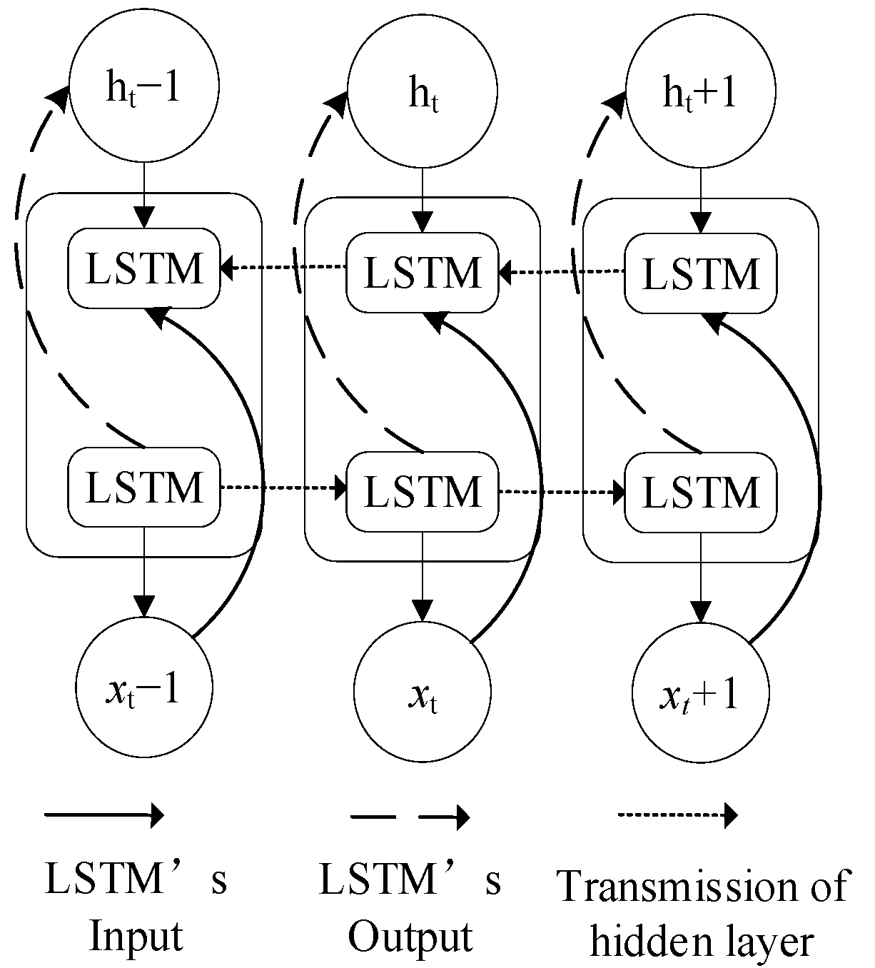
BiLSTM is an improved LSTM, which can be regarded as two single-layer LSTMs stacked together, and its structure is shown in Figure 3. The two LSTM inputs are the same, but the directions of information transmission are opposite. Therefore, BiLSTM is a modeling analysis of the entire time series. Compared with traditional LSTM, it comprehensively considers historical information and future information, and can enhance the forecasting ability [31].
In BiLSTM, the same input data are fed into the forward LSTM and the backward LSTM, respectively, to calculate the hidden state h t of the forward LSTM and the hidden state h t of the backward LSTM. Then, the two hidden states are connected and calculated to obtain the final output y t of BiLSTM:
h t = LSTM ( x t , h t 1 )
h t = LSTM ( x t , h t + 1 )
y t = W h y h t + W h y h t + b y
In which, W h y , W h y represents weights of forward LSTM and backward LSTM, respectively. by is the biased vector of the output layer.

3.4. CNN-BILSTM Network Structure

Usually, the performance of deep learning is closely related to the extracted features. CNN can filter key features and compress sequence length. BiLSTM can mine the time-series characteristics of data. So, combining CNN with BiLSTM is conducive to obtain deeper global features and their temporal relations.
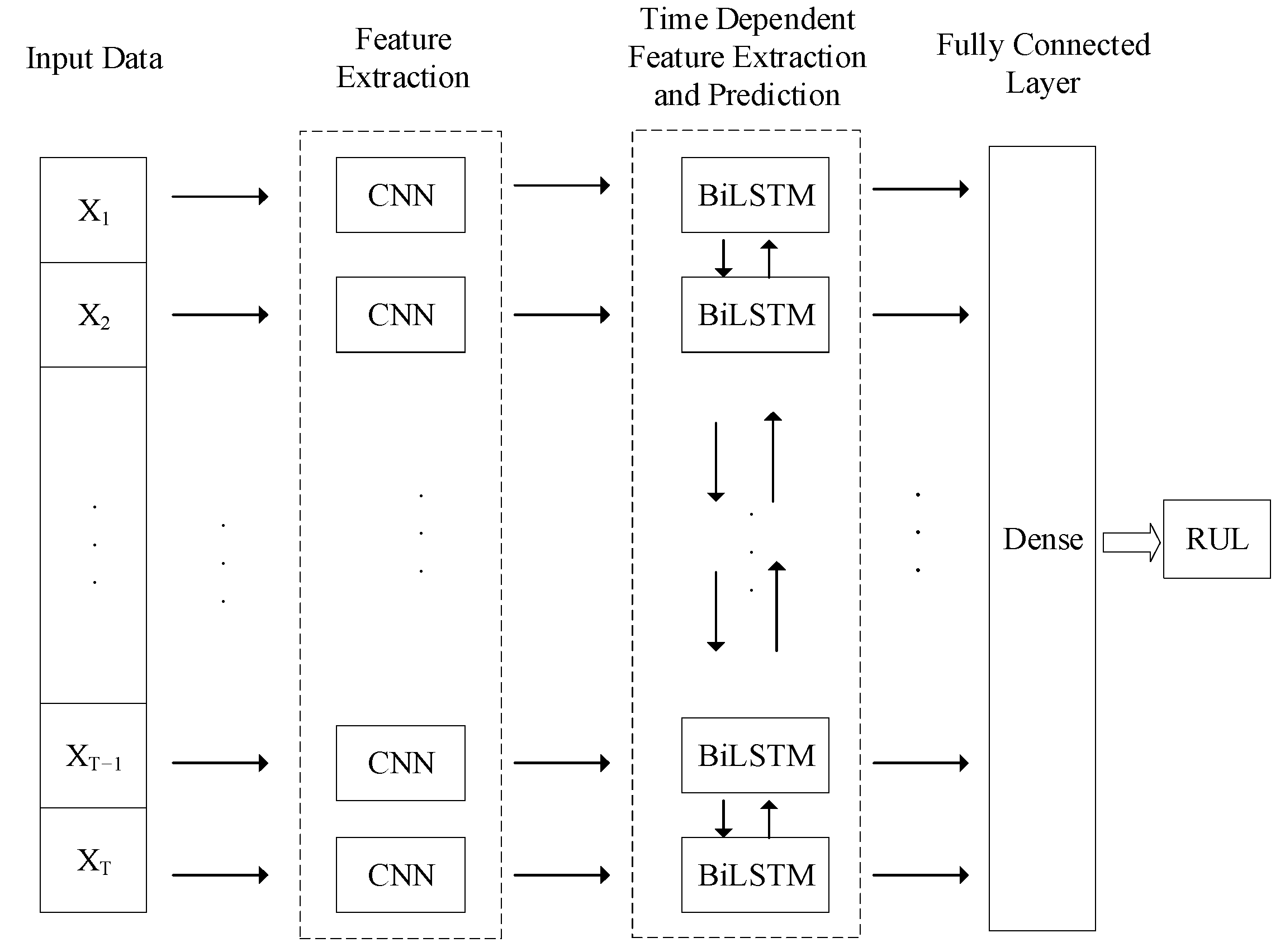
The CNN-BiLSTM model mainly includes four phases, shown as Figure 4. (1) In the input layer, the original data are preprocessed to obtain the input format required by the network, and the model is sequentially input along the time axis through the sliding window method. (2) Crucial deep global features are extracted through a single-layer convolutional layer, and then the sequence length is compressed by a single-layer max-pooling layer in order to extract and compress the data into more abstract features. (3) These features are used as the input of BiLSTM for deep mining and extraction of data time-series features. (4) The features are passed through a fully connected layer to obtain the final RUL prediction result.
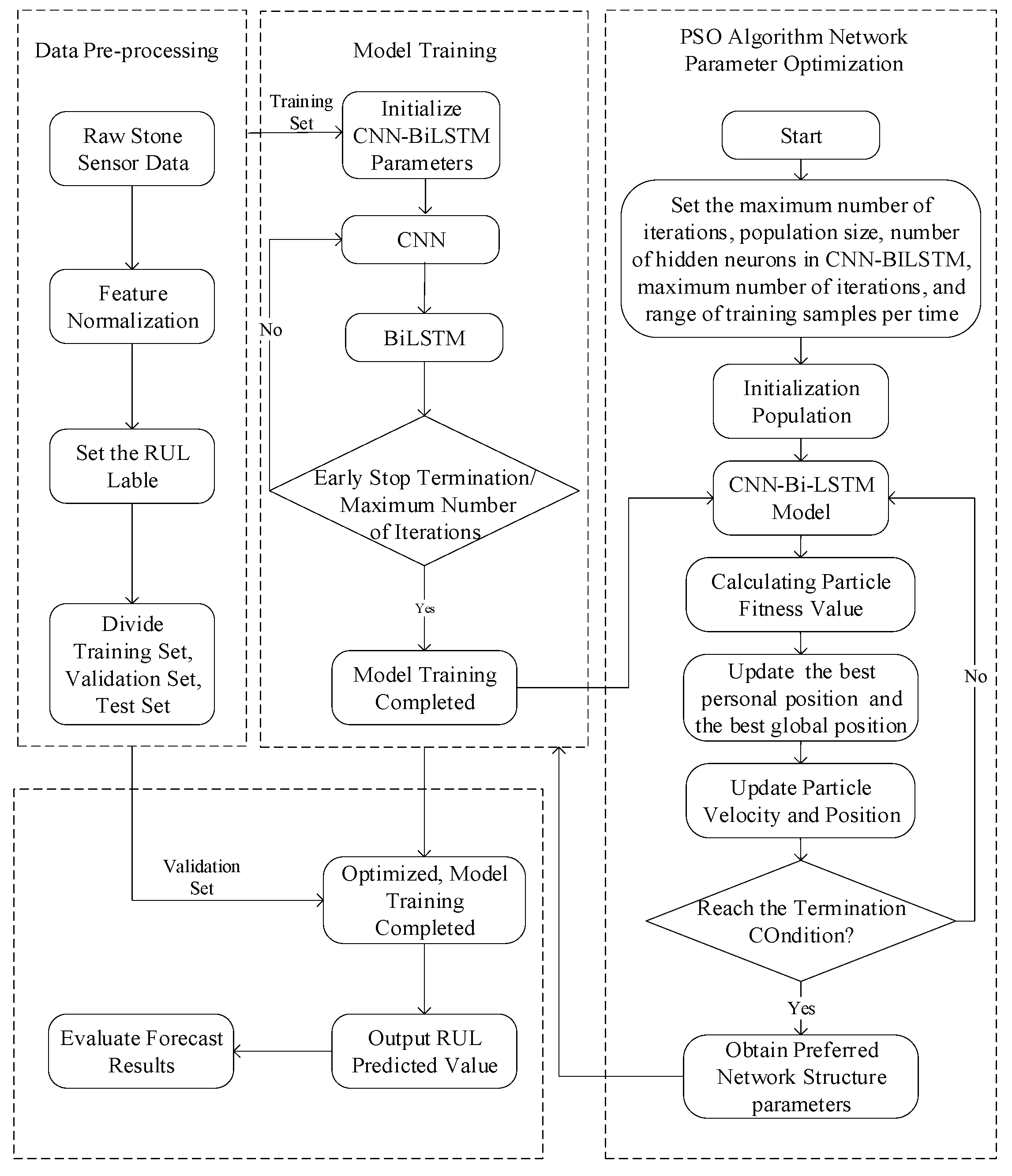
According to the basic network structure, the steps of remaining life prediction using the CNN-BiLSTM model are shown in Figure 5. It mainly includes data preprocessing, model training and RUL prediction.
(1) Data preprocessing
The original data usually come from different sensors, and the collected state data of the equipment are not the same. In order to eliminate the influence of the data dimensional difference, each eigenvalue is normalized to keep all the data in [0, 1]. After normalization, the RUL value at each time point needs to be calculated according to the full life cycle of the mechanical equipment. For example, when the mechanical equipment fails completely, the RUL value is 0, and the values at the other time points are derived by reversed chronological order in turn. After that, the data are divided into a training set, validation set and test set. The training set and validation set are used for model training, and the test set is used to predict and verify the accuracy of the model.
(2) Model training
The parameters of CNN and BiLSTM should be set before training, such as the number of convolutional layers and pooling layers of CNN, the size of the convolution kernel, the number of layers of BiLSTM, the number of neurons in the hidden layer, time step, maximum number of iterations, etc. After initializing the parameters, next follows determination of the loss function of the model, inputting the training set data and validation set data into the CNN to extract the local features of the data, and inputting the extracted features into the BiLSTM layer to mine its time-series characteristics. When reaching the termination condition, stopping the model training.
(3) RUL prediction
Inputting the test set data into the trained model, obtaining the RUL prediction result, and evaluating the prediction result.

3.5. Particle Swarm Optimization (PSO)

The particle swarm optimization algorithm (PSO) is used to complete the evolution of bird flocks through mutual assistance and information sharing among individuals. The PSO algorithm is similar to the process of bird feeding and is a heuristic evolutionary algorithm with good global optimization capability [32]. It is also widely used in the global optimization process of hyperparameters due to its simple principle and easy operation [33]. Assuming that there is only one optimal solution in a region D, the positions and velocities of m particles are initialized in the region. The positions of the particles represent the candidate solutions, while the velocities determine the motion of the particles. After initialization, the fitness of each particle can be calculated, as well as the personal best position P b e s t and the global best position G b e s t , and then the positions and velocities of the m particles are updated according to the following equation:
V i d k + 1 = w V i d k + c 1 r 1 ( P b e s t k x i d k ) + c 2 r 2 ( G best k x i d k )
X i d k + 1 = X i d k + V i d k + 1
where w denotes the inertia factor; c 1 , c 2 denote the acceleration factor of the example; r 1 , r 2 are random numbers between (0, 1); V i d k + 1 is the velocity vector of the ith particle motion in the (k+1)th iteration; and X i d k is the current position vector of the particle.
In this paper, the process of optimizing hyperparameters by PSO is as follows: firstly, set the number of particles m and the search range D, and initialize the position and velocity of particles within the range, round all parameters (number of neurons in the hidden layer, maximum number of iterations, number of samples in each training session) to the nearest integer, with each set of parameters corresponding to a particle, and the loss function of each training process in the neural network can be set to the particle’s fitness function. Then, the personal best position and global best position are updated according to the fitness of all particles, and the velocity and position of each particle can be updated by the new personal best position and global best position. Finally, the optimal hyperparameters are obtained from which the best hyperparameters are selected.

3.6. Tuning the Network Structure Parameters

In the network structure, the main hyperparameters that affect the performance of CNN-BiLSTM can be divided into two categories. One kind of parameters has a certain influence on the prediction performance of the model, such as the number of LSTM layers, learning rate and time window size. The other kind has no obvious effect on the prediction performance, such as the number of neurons in the hidden layer, the maximum number of iterations and the number of samples per training.
(1) The number of LSTM layers
BiLSTM is essentially a two-layer LSTM. In the case of sufficient sample data, stacking LSTM and deepening the structure of the network may bring better fitting results, but the increase in the number of layers will also bring the burden of computing time and memory consumption. When the number of LSTM layers is too large, it may appear that the iteration becomes slower, which makes the model convergence effect worse, resulting in falling into a local optimal solution. Therefore, it is necessary to find a reasonable number of LSTM layers.
(2) Learning rate
In deep learning, the learning rate is an important parameter that can control the learning progress. When the learning rate is large, the convergence rate of the prediction model will be faster, and exploding gradient may occur. When the learning rate is small, the convergence rate will be slower, which is prone to overfitting problems. Therefore, it is necessary to set a larger learning rate at the beginning of training, and reduce it in the later stage of training. A learning rate adaptive optimization algorithm is generally used to automatically optimize the learning rate, such as Adadelta, Adagrad, Adam, Momentum, etc.
(3) Time window size
In the training process of the deep learning model, the sliding time window method is widely used to input sample data to the model. The time window size can significantly affect the predictive performance of the model. In general, the larger the time window, the more useful information it contains, and the better the prediction effect of the model will be.
(4) The number of neurons in the hidden layer, the maximum number of iterations and the number of samples for each training.
The influence of one of these hyperparameters on the model performance is not obvious, but the coupling effect between these different hyperparameters affects the performance of the network. In order to find a set of better parameter values, this paper uses a particle swarm optimization algorithm [34] to tune this set of hyperparameters. The prediction process is shown in Figure 6.
The PSO-CNN-BiLSTM residual lifetime prediction model proposed in this paper requires more time for parameter optimization and network training than the ordinary model in the training phase due to its complex architectural design and optimization strategy, but once the model training is completed, its prediction speed is not slower than that of the ordinary model, and the time required for both of them to perform the prediction task is basically equivalent. Therefore, considering the advantages of the PSO-CNN-BiLSTM model in prediction performance, the extra training time invested in the early stages is undoubtedly worthwhile.

4. Example Analysis

In order to verify the effectiveness of CNN-BiLSTM method in predicting the RUF, the PHM08 dataset was used to test the performance of multiple prediction models such as LSTM, BiLSTM, multi-layer LSTM and CNN-BiLSTM. Meanwhile, the number of LSTM layers, learning rate, time window size, the number of hidden layer neurons, the maximum number of iterations and the number of training samples were optimized to improve the prediction performance of CNN BiLSTM model. To ensure the consistency of the experiments, the experimental equipment used in this paper was a general PC with Intel(R) Core(TM) i7-8750 CPU and 16 GB of operating memory.

4.1. Preprocessing of Raw Data

The PHM08 dataset used in this paper was provided by NASA, which is one of the most widely used remaining life prediction datasets. It includes 218 pieces of complete life cycle data of the same type of aircraft turbine engines from operation to failure, but the health level of each engine at the beginning of operation is different. There are 26 columns in the original data. The first two columns represent the equipment ID and the current operation cycle time. The third to fifth columns are the operating status of the equipment. The rest are the status monitoring data collected by the smart sensors installed in the device, as shown in Table 1.
Each piece of equipment has a different fitness level before starting, so the time required for its operation to failure is also different. The dataset covers the complete cycle of equipment operation. The specific values of the original data are shown in Table 2.
In order to eliminate the influence of dimension difference between features, the original data are processed by maximum and minimum normalization, and all selected features are normalized.
x * = x x min x max x min
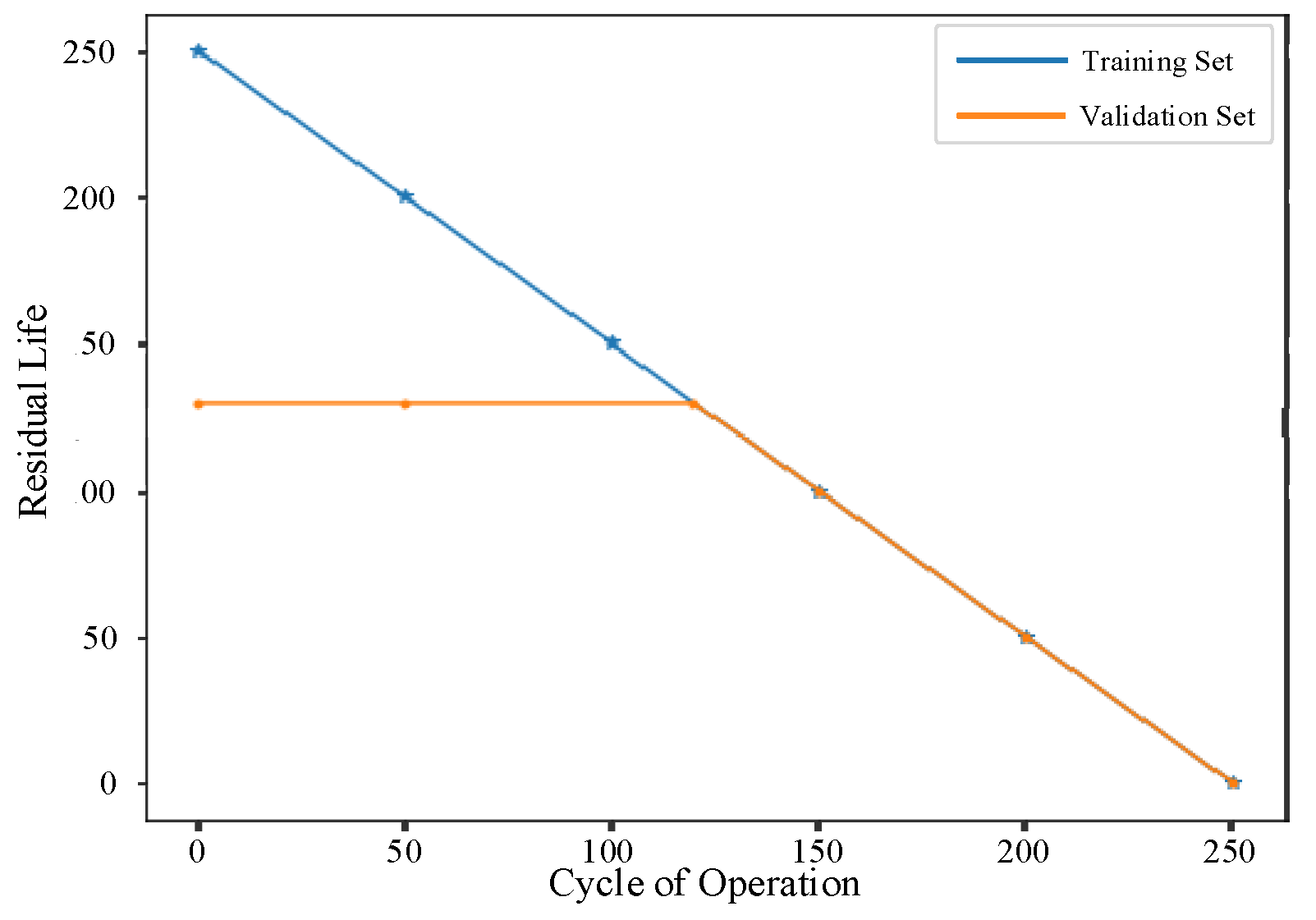
After normalization, the data are labeled and the RUL at each time point is calculated. Considering that the engine performance is in a healthy state at the beginning of operation, an accurate prediction result cannot always be obtained, if the RUL label is set directly according to the current and total operating cycles. Therefore, the training label is usually corrected with a piecewise linear function. Setting the maximum RUL value to 130. If the operation cycle is greater than 130, the RUL label will remain unchanged. On the contrary, if the operation cycle is less than 130, the RUL will decrease linearly with the increase in the operation cycle, as shown in Figure 7.
The data after normalization and RUL label setting are shown in Table 3, where RUL represents the remaining life at this time point.

4.2. Result Analysis

First, comparing LSTM and BiLSTM prediction models. Initialize the parameters of the LSTM and BiLSTM models. Set the number of hidden layer neurons to 50, the size of the time window to 50, the maximum number of iterations to 200 and the number of training samples to 200. The learning rate optimization algorithm is Adam, and the activation function is ReLU. The mean absolute error (MAE) is selected as the loss function, and the early stopping method is added to the model to reduce the training time of the model and prevent over fitting. The final prediction results use MAE, root mean square error (RMSE) and R-Square (R2) as the evaluation criteria, respectively. The MAE, RMSE and R2 can be expressed as:
M A E = 1 m i = 1 m | y ^ i y i |
R M S E = 1 m i = 1 m ( y i ^ y i ) 2
R 2 = 1 i ( y i y ^ i ) 2 i ( y i y ¯ ) 2
In which, yi, ŷi and y ¯ are the theoretical value, predicted value and actual average value of RUL, respectively.
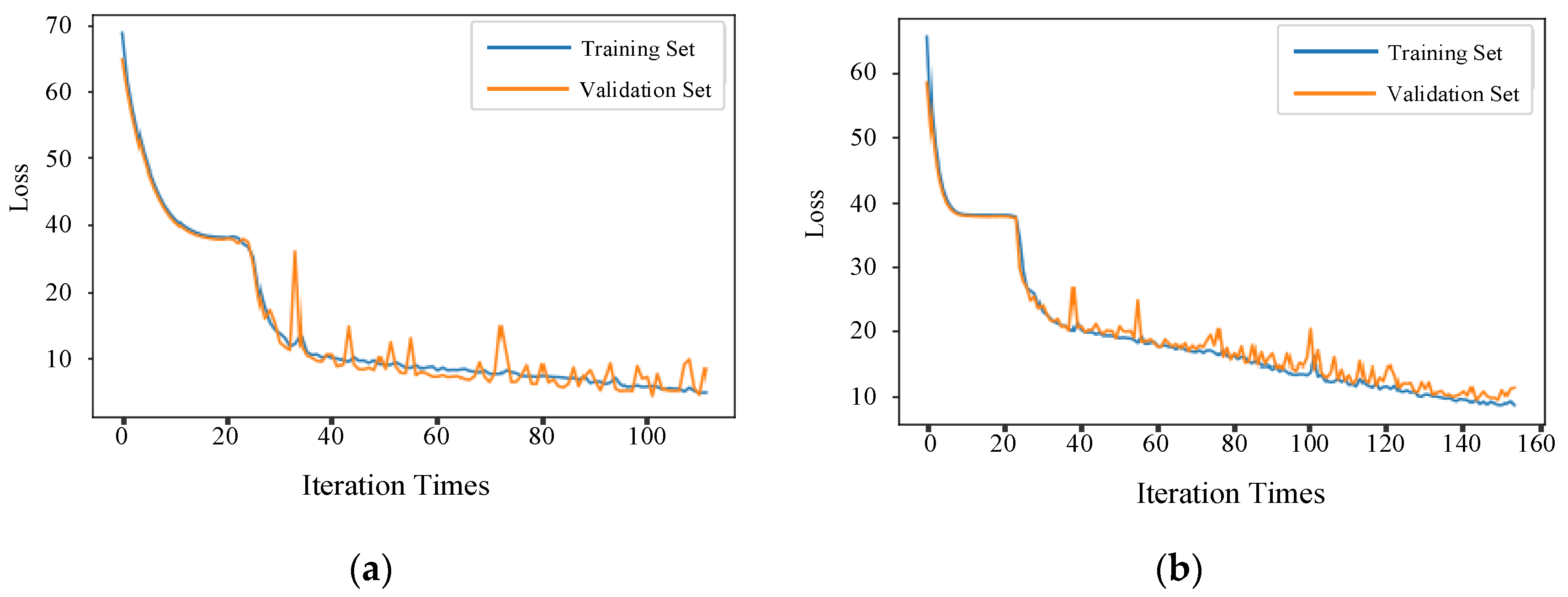
The loss function comparison results of the LSTM model and BiLSTM model are shown in Figure 8. When using the LSTM model, the model stops training after 113 iterations, while the BiLSTM model stops training after 157 iterations due to the more complex network structure. Compared with LSTM, BiLSTM takes longer to train, but the loss decreases more, and the convergence effect is better.
Using MAE, RMSE and R2 to evaluate the prediction results. In order to eliminate the influence of error, the average value of three prediction results is taken for statistical analysis, and the final evaluation results are shown in Table 4. Using BiLSTM can achieve a better prediction effect.
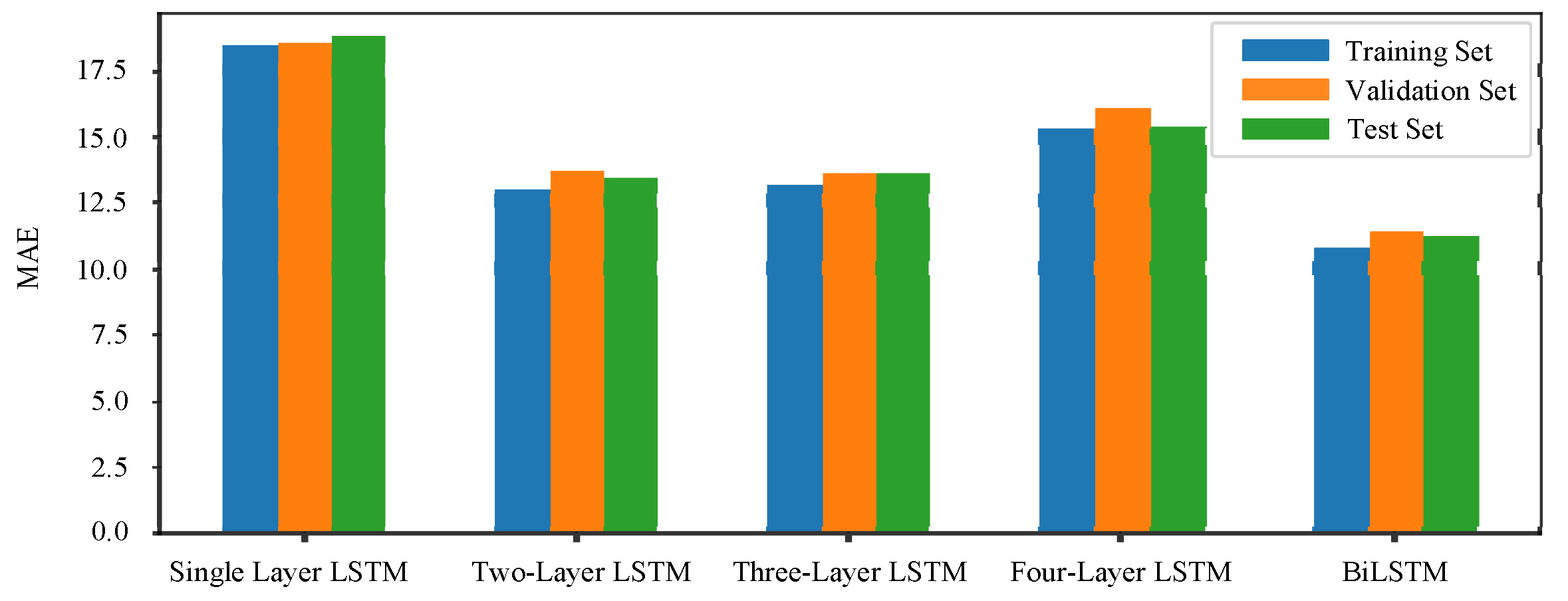
In general, stacking multiple LSTMs may also improve the performance of the LSTM model. To explore the performance of a multi-layer LSTM and BiLSTM, a total of five sets of models for one to four layers of LSTM and BiLSTM are compared using the above datasets. Each model experiment is run three times and the average is taken to obtain the final MAE, as shown in Figure 9.
It can be found that the MAE value of a two-layer LSTM is lower than that of single-layer LSTM. However, when the LSTM layers continue to stack to the third or fourth layers, the MAE value does not change much compared with that of the two-layer LSTM. A small number of stacked LSTM network structures will improve the predictive accuracy of the RUL regression model, but the predictive accuracy of the model tends to stabilize as the LSTM layers continue to increase. The MAE of BiLSTM is lower than that of multi-layer LSTM. Therefore, in the RUL forecasting problem, the BiLSTM structure can better mine valuable time information from raw data than the multi-layer LSTM network structure, and the regression forecasting effect is better.
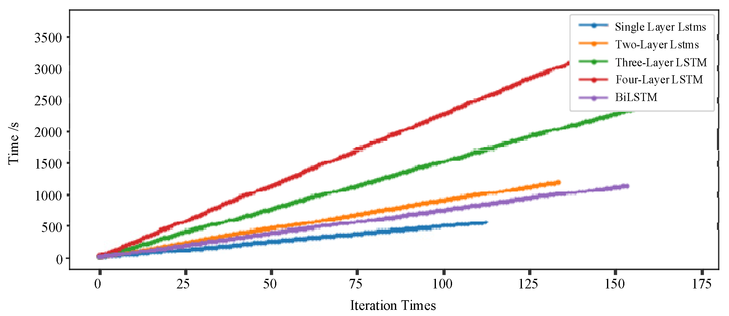
During the training, it is found that with LSTM stacking and network structure complicating, the regression model becomes more and more difficult to converge, and the prediction time increases. The training time of BiLSTM model is shorter than that of stacked LSTM, which is shown in Figure 10.
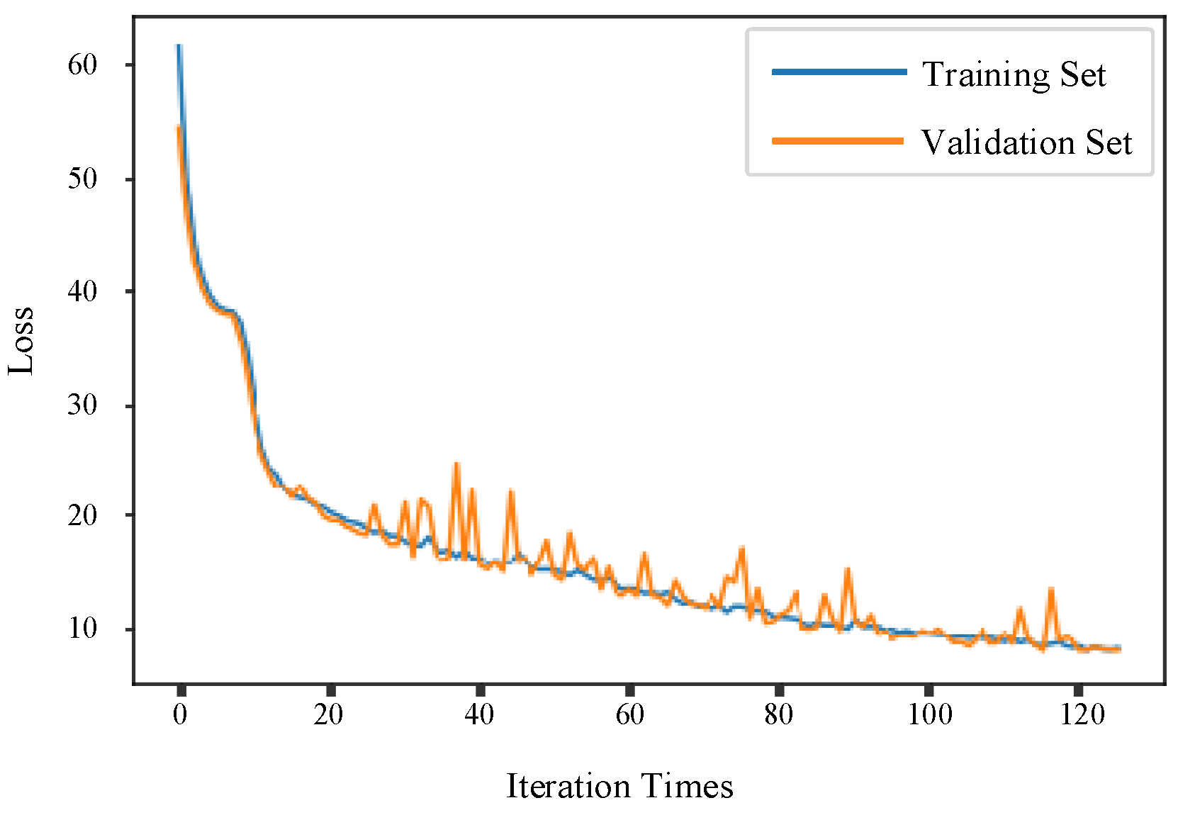
In order to further improve the BiLSTM feature extraction ability, a convolution layer and a maximum pooling layer are added to the BiLSTM to extract deep spatial features and retain the best features in the original data. The new model called CNN-BiLSTM stops iterating at 126 times. The loss function of CNN-BiLSTM decreases faster and fluctuates less than that of BiLSTM for the training set and verification set, as shown in Figure 11.
The average evaluation results of the CNN-BiLSTM model are shown in Table 5. The prediction effect has been significantly improved after improving BiLSTM with CNN.
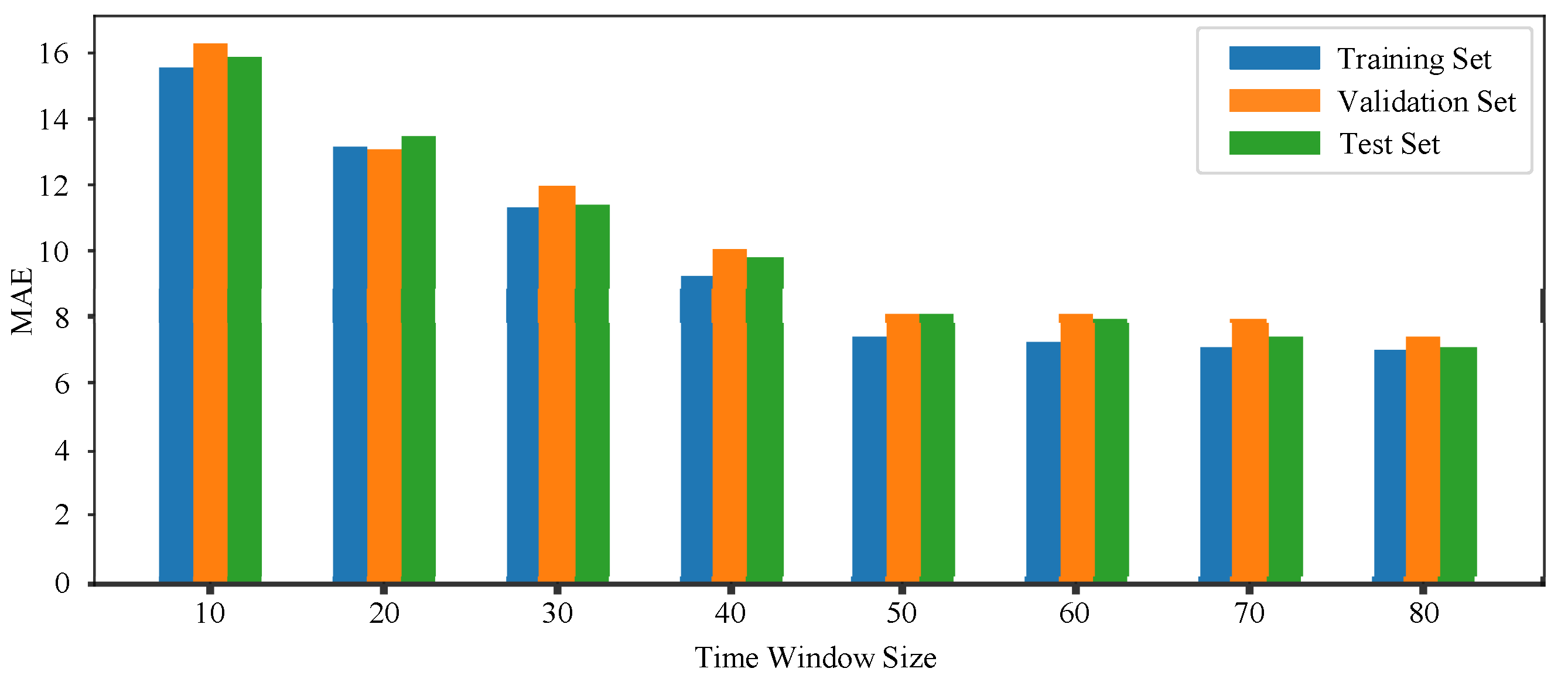
For optimizing the CNN-BiLSTM hyperparameters, the influence of different time window sizes is verified on the prediction performance of the model. The time window sizes 10, 20, 30, 40, 50, 60, 70, and 80 are used in comparative experiments, respectively. Each size experiment is run three times, and MAE takes the average of three sets of experimental results, as shown in Figure 12.
It is observed that when the time window size increases from 10 to 50, the MAE of the prediction error decreases rapidly. When the time window size exceeds 50, the MAE decline is not obvious. So, in the subsequent model prediction performance test, the time window size of the prediction model is set to 50.
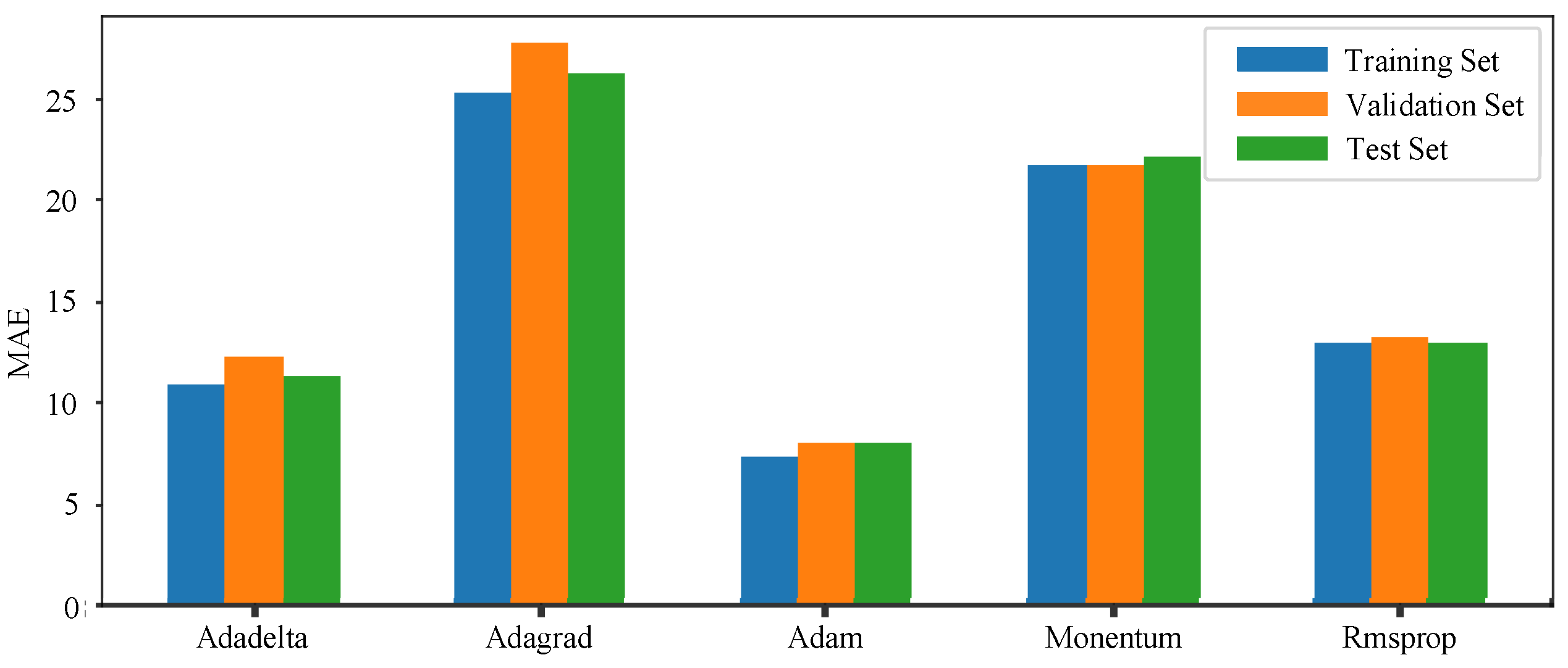
The comparison experiments of different algorithms are carried out for the learning rate optimization. The result is shown in Figure 13, which indicates that the Adam is a more suitable learning rate optimization algorithm.
Use PSO to optimize the number of neurons in the hidden layer of the model, the maximum number of iterations, and the number of training samples. The value range of three variables are set as the following: number of hidden layer neurons is in [1, 200], maximum number of iterations is in [100, 500] and number of training samples is in [50, 500]. The vector formed by these three parameters is regarded as the particle position in PSO, and the number of particles is 50, the inertia factor is 0.5 and acceleration factor is 2. The MAE of CNN-BiLSTM is used as the fitness value of PSO. The MAE value of the training set on the CNN-BiLSTM model is 7.34 before PSO optimization. In order to reduce the training time of the model, stop training when the optimized MAE is less than 5 or the number of iterations reaches the maximum 200.
After PSO optimization, the hyperparameters of the model are: the number of hidden layer neurons is 64, the maximum number of iterations is 287 and the number of training samples is 254. By comparing the various evaluation metrics, the prediction results of the improved PSO-CNN-BiLSTM model are shown in Table 6. Finally, when comparing the performance of LSTM, BiLSTM, CNN-BiLSTM and PSO-CNN-BiLSTM models on the test set, the PSO-CNN-BiLSTM model exhibits more excellent prediction results, as shown in Table 7.
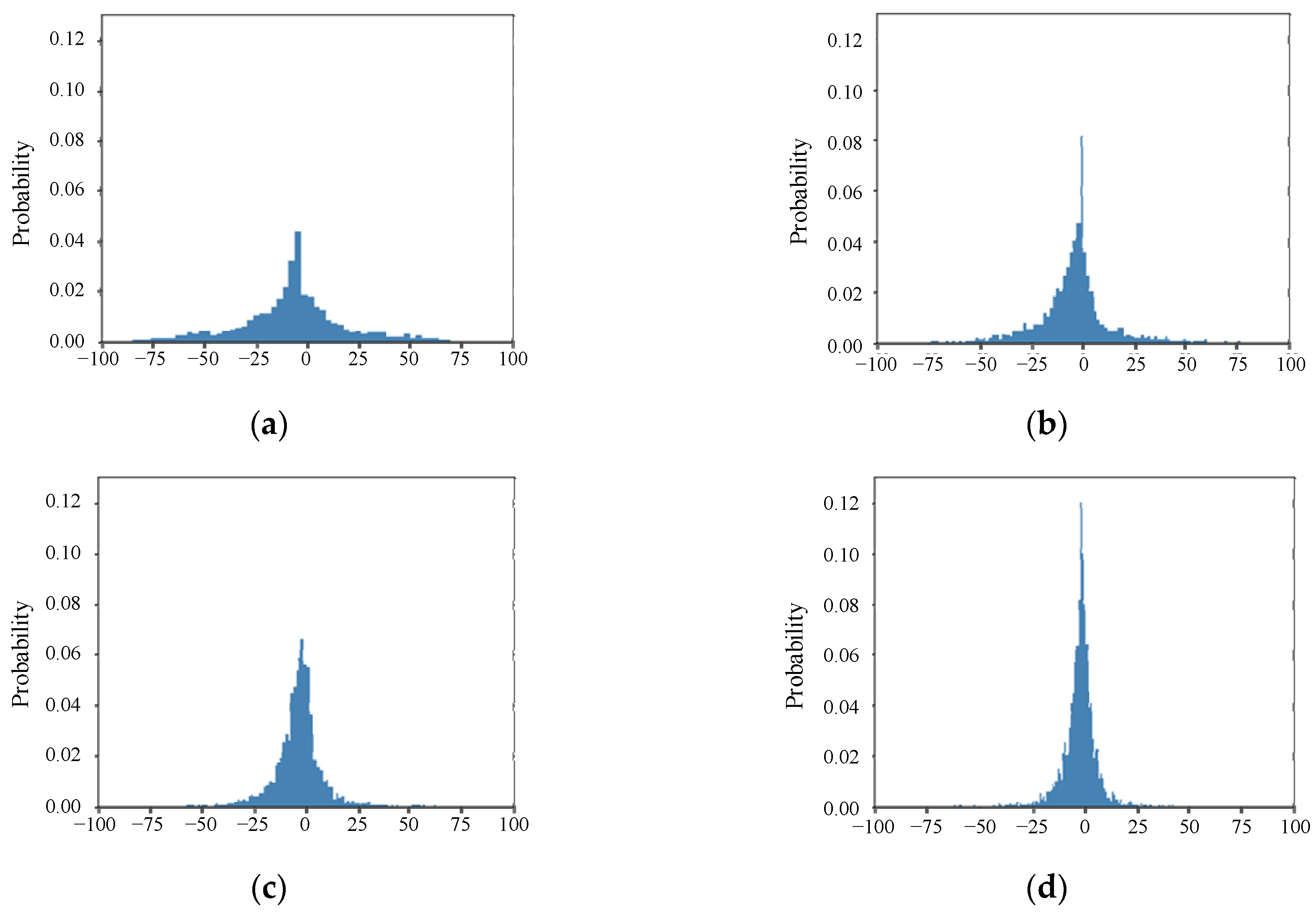
The prediction error distribution of the four models LSTM, BiLSTM, CNN-BiLSTM and PSO-CNN-BiLSTM on the test set is shown in Figure 14. The PSO-CNN-BiLSTM model has the smallest error and the best prediction effect.
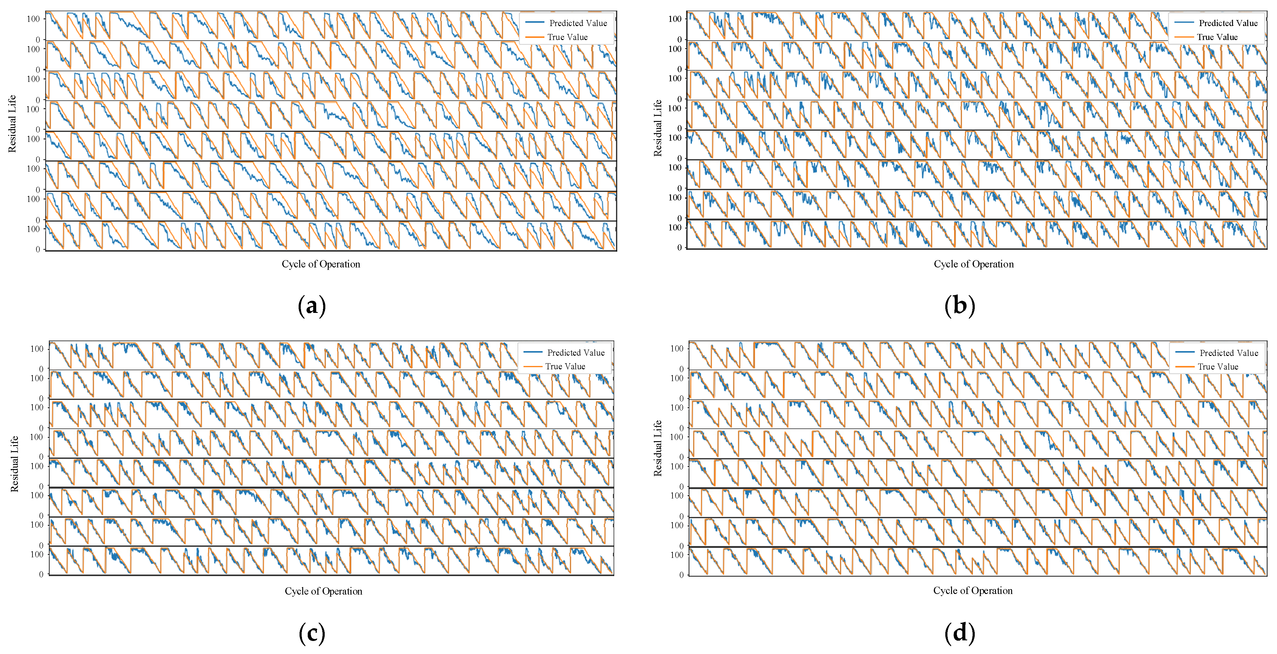
Input the data of 218 pieces of equipment into four models LSTM, BiLSTM, CNN-BiLSTM and PSO-CNN-BiLSTM, respectively, to obtain the comparison between the predicted value and the true value of the model. The results are shown in Figure 15. Each sawtooth wave in the figure represents the complete life cycle of a turbine engine from start to failure. The orange line represents the true value, and the blue line represents the predicted value.
Comparing the results of the four models, the prediction results of PSO-CNN-BiLSTM are the closest to the true values, followed by CNN-BiLSTM, and then BiLSTM. LSTM has the worst prediction effect. In order to compare the prediction performance of the four models in detail, the RUL of one of the 218 devices is predicted by using the models. The results are shown in Figure 16. The prediction result of the PSO-CNN-BiLSTM model with adjusted network hyperparameters is closer to the true value.
In order to evaluate the performance of the model proposed in this paper on test data, the quality of the model is measured using the Score function proposed in the International PHM Conference in the PHM08 Data Challenge [35]. The scoring function is shown in Equation (18), which (Score) is an asymmetric function that penalizes more heavily when the prediction is late than when the prediction is early. Specifically, when the model-estimated remaining useful life (RUL) is lower than the actual value, the penalty is relatively light and is unlikely to trigger a serious system failure because there is still enough time for equipment maintenance. However, if the model-estimated RUL exceeds the actual value, maintenance schedules will be delayed, which may increase the risk of system failure, and therefore the penalty in this case will be more severe. This asymmetric scoring mechanism is intended to guide the model to be more cautious in its predictions in order to avoid potential risks due to inaccuracies in maintenance schedules.
S c o r e = i = 1 R s i , s i = { e ( R U L p r e d ) i ( R U L a c t u a l ) i 13 1 ,         for ( R U L p r e d ) i ( R U L a c t u a l ) i < 0 e ( R U L p r e d ) i ( R U L a c t u a l ) i 10 1 ,             for ( R U L p r e d ) i ( R U L a c t u a l ) i 0
where ( R U L p r e d ) i and ( R U L a c t u a l ) i represent the predicted and actual RUL of the ith sample in the test dataset.
We have computed the prediction results of our lifetime prediction model using a specific scoring function (Equation (18)) and made a comparison with CNN, LSTM and other lifetime prediction methods in the literature. Table 8 shows the score results.
After comparing the scores with other residual lifetime prediction methods, our proposed PSO-CNN-BiLSTM model is better at predicting the PHM08 dataset.

5. Conclusions

Aiming at the strong temporal correlation of operating data in the degradation process of mechanical equipment, a PSO-CNN-BiLSTM model of RUL prediction was constructed. In the model, CNN was used as a feature extractor for deep extraction and compression of features, and BiLSTM was used as a time-series processing tool to fully exploit the sequential characteristics in the life cycle data of mechanical equipment. For the hyperparameter optimization problem in the model training, considering the influence of LSTM layer number, learning rate and time window size on the performance of the prediction model, the optimal LSTM layer number, learning rate optimization algorithm and time window size were selected for specific experimental objects. The PSO was used to optimize the three important parameters of the neural network model (the number of hidden neurons, the number of iterations and the number of input samples for each training). Finally, the PSO-CNN-BiLSTM RUL prediction model was constructed and verified based on the aero-engine PHM08 dataset. The results show that the PSO-CNN-BiLSTM model has a better prediction effect and overall performance than the LSTM, BiLSTM and CNN-BiLSTM models.

Author Contributions

Y.L.: conceptualization, methodology, validation, writing—original draft, writing—review and editing; J.L.: data curation, formal analysis, software, validation, visualization, writing—original draft; H.W.: software, validation, visualization; M.Y.: conceptualization, supervision, writing—review and editing; X.G.: supervision, writing—review and editing; S.L.: supervision, writing—review and editing. All authors have read and agreed to the published version of the manuscript.

Funding

This research was funded by the Key Research and Development Program of Shaanxi (Program No. 2021SF-421, 2021SF-422), the Key Scientific Research Program of Shaanxi Provincial Education Department (Program No. 20JY047), and the Collaborative Innovation Center of Modern Equipment Green Manufacturing in Shaanxi Province, China.

Institutional Review Board Statement

Not applicable.

Informed Consent Statement

Not applicable.

Data Availability Statement

Due to the nature of this research, participants of this study did not agree for their data to be shared publicly, so supporting data are not available.

Conflicts of Interest

The authors declare that they have no known competing financial interests or personal relationships that could have appeared to influence the work reported in this paper.

References

  1. Vogl, G.W.; Weiss, B.A.; Helu, M. A review of diagnostic and prognostic capabilities and best practices for manufacturing. J. Intell. Manuf. 2019, 30, 79–95. [Google Scholar] [CrossRef] [PubMed]
  2. Qian, Y.; Yan, R.; Gao, R.X. A multi-time scale approach to remaining useful life prediction in rolling bearing. Mech. Syst. Signal Process. 2017, 83, 549–567. [Google Scholar] [CrossRef]
  3. Zhai, Q.; Ye, Z.-S. RUL Prediction of Deteriorating Products Using an Adaptive Wiener Process Model. IEEE Trans. Ind. Inform. 2017, 13, 2911–2921. [Google Scholar] [CrossRef]
  4. Meng, H.; Li, Y.-F. A review on prognostics and health management (PHM) methods of lithium-ion batteries. Renew. Sustain. Energy Rev. 2019, 116, 109405. [Google Scholar] [CrossRef]
  5. Zhang, J.; Wang, J.; Lyu, Y.; Bao, J. Big Data Driven Intelligent Manufacturing. China Mech. Eng. 2019, 30, 127. [Google Scholar]
  6. Zhou, Y.; Wang, Z.; Zuo, X.; Zhao, H. Identification of wear mechanisms of main bearings of marine diesel engine using recurrence plot based on CNN model. Wear 2023, 520–521, 204656. [Google Scholar] [CrossRef]
  7. Lee, H.; Jeong, H.; Koo, G.; Ban, J.; Kim, S.W. Attention Recurrent Neural Network-Based Severity Estimation Method for Interturn Short-Circuit Fault in Permanent Magnet Synchronous Machines. IEEE Trans. Ind. Electron. 2021, 68, 3445–3453. [Google Scholar] [CrossRef]
  8. Han, S.-R.; Kim, Y.-S. A fault identification method using LSTM for a closed-loop distribution system protective relay. Int. J. Electr. Power Energy Syst. 2023, 148, 108925. [Google Scholar] [CrossRef]
  9. Yan, H.; Wan, J.; Zhang, C.; Tang, S.; Hua, Q.; Wang, Z. Industrial Big Data Analytics for Prediction of Remaining Useful Life Based on Deep Learning. IEEE Access 2018, 6, 17190–17197. [Google Scholar] [CrossRef]
  10. Jiao, J.; Zhao, M.; Lin, J.; Liang, K. A comprehensive review on convolutional neural network in machine fault diagnosis. Neurocomputing 2020, 417, 36–63. [Google Scholar] [CrossRef]
  11. Yang, B.; Liu, R.; Zio, E. Remaining Useful Life Prediction Based on a Double-Convolutional Neural Network Architecture. IEEE Trans. Ind. Electron. 2019, 66, 9521–9530. [Google Scholar] [CrossRef]
  12. Wang, B.; Lei, Y.; Yan, T.; Li, N.; Guo, L. Recurrent convolutional neural network: A new framework for remaining useful life prediction of machinery. Neurocomputing 2020, 379, 117–129. [Google Scholar] [CrossRef]
  13. Bae, J.; Xi, Z. Learning of physical health timestep using the LSTM network for remaining useful life estimation. Reliab. Eng. Syst. Saf. 2022, 226, 108717. [Google Scholar] [CrossRef]
  14. Xiang, S.; Qin, Y.; Luo, J.; Pu, H.; Tang, B. Multicellular LSTM-based deep learning model for aero-engine remaining useful life prediction. Reliab. Eng. Syst. Saf. 2021, 216, 107927. [Google Scholar] [CrossRef]
  15. Li, H.; Wang, Z.; Li, Z. An enhanced CNN-LSTM remaining useful life prediction model for aircraft engine with attention mechanism. PeerJ Comput. Sci. 2022, 8, e1084. [Google Scholar] [CrossRef]
  16. Shi, P.; Hong, L.; He, D. Using Long Short Term Memory Based Approaches for Carbon Steel Fatigue Remaining Useful Life Prediction. In Proceedings of the 2018 Prognostics and System Health Management Conference (PHM-Chongqing), Chongqing, China, 26–28 October 2018; pp. 1055–1060. [Google Scholar]
  17. Marei, M.; Li, W. Cutting tool prognostics enabled by hybrid CNN-LSTM with transfer learning. Int. J. Adv. Manuf. Technol. 2022, 118, 817–836. [Google Scholar] [CrossRef]
  18. Zhou, Z.; Yang, L.; Wang, Z.; Yao, Y. Remaining Useful Life Prediction of Aero-Engine using CNN-LSTM and mRMR Feature Selection. In Proceedings of the 2022 4th International Conference on System Reliability and Safety Engineering (SRSE), Guangzhou, China, 15–18 December 2022; pp. 41–45. [Google Scholar]
  19. Li, X.; Zhang, L.; Wang, Z.; Dong, P. Remaining useful life prediction for lithium-ion batteries based on a hybrid model combining the long short-term memory and Elman neural networks. J. Energy Storage 2019, 21, 510–518. [Google Scholar] [CrossRef]
  20. Al-Dulaimi, A.; Zabihi, S.; Asif, A.; Mohammadi, A. Hybrid Deep Neural Network Model for Remaining Useful Life Estimation. In Proceedings of the ICASSP 2019—2019 IEEE International Conference on Acoustics, Speech and Signal Processing (ICASSP), Brighton, UK, 12–17 May 2019; pp. 3872–3876. [Google Scholar]
  21. Zhao, C.; Huang, X.; Li, Y.; Li, S. A Novel Cap-LSTM Model for Remaining Useful Life Prediction. IEEE Sens. J. 2021, 21, 23498–23509. [Google Scholar] [CrossRef]
  22. Droste, S.; Jansen, T.; Wegener, I. Upper and Lower Bounds for Randomized Search Heuristics in Black-Box Optimization. Theory Comput. Syst. 2006, 39, 525–544. [Google Scholar] [CrossRef]
  23. Lu, W.; Cai, B.; Gu, R. Improved Particle Swarm Optimization Based on Gradient Descent Method. In Proceedings of the 4th International Conference on Computer Science and Application Engineering, Sanya, China, 20–22 October 2020; Association for Computing Machinery: New York, NY, USA, 2020; pp. 1–6. [Google Scholar]
  24. Salih, O.; Duffy, K.J. Optimization Convolutional Neural Network for Automatic Skin Lesion Diagnosis Using a Genetic Algorithm. Appl. Sci. 2023, 13, 3248. [Google Scholar] [CrossRef]
  25. Zhang, X.; Jiang, Y.; Zhong, W. Prediction Research on Irregularly Cavitied Components Volume Based on Gray Correlation and PSO-SVM. Appl. Sci. 2023, 13, 1354. [Google Scholar] [CrossRef]
  26. Badiger, P.V.; Desai, V.; Ramesh, M.R.; Prajwala, B.K.; Raveendra, K. Cutting Forces, Surface Roughness and Tool Wear Quality Assessment Using ANN and PSO Approach During Machining of MDN431 with TiN/AlN-Coated Cutting Tool. Arab. J. Sci. Eng. 2019, 44, 7465–7477. [Google Scholar] [CrossRef]
  27. Jidong, Z.; Yisheng, Z.O.U.; Jialin, D.; Xiaolu, Z. Bearing Remaining Life Prediction Based on Full Convolutional Layer Neural Networks. China Mech. Eng. 2019, 30, 2231. [Google Scholar]
  28. Zhao, C.; Huang, X.; Li, Y.; Yousaf Iqbal, M. A Double-Channel Hybrid Deep Neural Network Based on CNN and BiLSTM for Remaining Useful Life Prediction. Sensors 2020, 20, 7109. [Google Scholar] [CrossRef]
  29. Yang, C.; Kong, X.; Wang, X. Model-Based Fault Diagnosis for Performance Degradations of Turbofan Gas Path via Optimal Robust Residuals. In Proceedings of the ASME Turbo Expo 2016: Turbomachinery Technical Conference and Exposition. Volume 6: Ceramics; Controls, Diagnostics and Instrumentation; Education; Manufacturing Materials and Metallurgy, Seoul, Republic of Korea, 13–17 June 2016; American Society of Mechanical Engineers Digital Collection. ASME: New York, NY, USA, 2016. [Google Scholar]
  30. NASA Ames Prognostics Data Repository, NASA Ames Research Center. Available online: https://ti.arc.nasa.gov/tech/dash/groups/pcoe/prog-nostic-data-repository/ (accessed on 1 December 2022).
  31. Almogren, A.S. Intrusion detection in Edge-of-Things computing. J. Parallel Distrib. Comput. 2020, 137, 259–265. [Google Scholar] [CrossRef]
  32. Feng, H.; Zhou, Y.; Zeng, W.; Guo, W. A physics-based PSO-BPNN model for civil aircraft noise assessment. Appl. Acoust. 2024, 221, 109992. [Google Scholar] [CrossRef]
  33. Shi, J.; Zhang, Y.; Sun, Y.; Cao, W.; Zhou, L. Tool life prediction of dicing saw based on PSO-BP neural network. Int. J. Adv. Manuf. Technol. 2022, 123, 4399–4412. [Google Scholar] [CrossRef]
  34. Chouikhi, N.; Ammar, B.; Rokbani, N.; Alimi, A.M. PSO-based analysis of Echo State Network parameters for time series forecasting. Appl. Soft Comput. 2017, 55, 211–225. [Google Scholar] [CrossRef]
  35. Behera, S.; Misra, R. Generative adversarial networks based remaining useful life estimation for IIoT. Comput. Electr. Eng. 2021, 92, 107195. [Google Scholar] [CrossRef]
  36. Sateesh Babu, G.; Zhao, P.; Li, X.-L. Deep Convolutional Neural Network Based Regression Approach for Estimation of Remaining Useful Life. In Database Systems for Advanced Applications; Navathe, S.B., Wu, W., Shekhar, S., Du, X., Wang, X.S., Xiong, H., Eds.; Springer International Publishing: Cham, Switzerland, 2016; pp. 214–228. [Google Scholar]
  37. Zheng, S.; Ristovski, K.; Farahat, A.; Gupta, C. Long Short-Term Memory Network for Remaining Useful Life estimation. In Proceedings of the 2017 IEEE International Conference on Prognostics and Health Management (ICPHM), Dallas, TX, USA, 19–21 June 2017; pp. 88–95. [Google Scholar]
  38. Song, T.; Liu, C.; Wu, R.; Jin, Y.; Jiang, D. A hierarchical scheme for remaining useful life prediction with long short-term memory networks. Neurocomputing 2022, 487, 22–33. [Google Scholar] [CrossRef]
  39. Chen, Z.; Wu, M.; Zhao, R.; Guretno, F.; Yan, R.; Li, X. Machine Remaining Useful Life Prediction via an Attention-Based Deep Learning Approach. IEEE Trans. Ind. Electron. 2021, 68, 2521–2531. [Google Scholar] [CrossRef]
  40. ElDali, M.; Kumar, K.D. Fault Diagnosis and Prognosis of Aerospace Systems Using Growing Recurrent Neural Networks and LSTM. In Proceedings of the 2021 IEEE Aerospace Conference (50100), Big Sky, MT, USA, 6–13 March 2021; pp. 1–20. [Google Scholar]
Figure 1. Key components of aircraft turbine engines.
Machines 12 00342 g001
Figure 2. The internal structure of an LSTM.
Machines 12 00342 g002
Figure 3. Structure of BiLSTM.
Machines 12 00342 g003
Figure 4. CNN-BiLSTM network structure.
Machines 12 00342 g004
Figure 5. CNN-BiLSTM prediction process.
Machines 12 00342 g005
Figure 6. PSO-CNN-BiLSTM prediction process.
Machines 12 00342 g006
Figure 7. RUL of turbine engine section.
Machines 12 00342 g007
Figure 8. Comparison of model loss functions. (a) Loss function of LSTM and (b) loss function of BiLSTM.
Machines 12 00342 g008
Figure 9. The comparison results of MAE of different models.
Machines 12 00342 g009
Figure 10. The comparison results of training time of different models.
Machines 12 00342 g010
Figure 11. Loss function of CNN-BiLSTM model.
Machines 12 00342 g011
Figure 12. MAE value of models with different time window sizes.
Machines 12 00342 g012
Figure 13. Comparison of MAE results for different learning rate optimization algorithms.
Machines 12 00342 g013
Figure 14. Error distribution diagram. (a) The regression model error of LSTM; (b) the regression model error of BiLSTM; (c) the regression model error of CNN-BiLSTM and (d) the regression model error of PSO-CNN-BiLSTM.
Machines 12 00342 g014
Figure 15. Comparison results of four prediction models. (a) Comparison of predicted and actual values of LSTM; (b) comparison of predicted and actual values of BiLSTM; (c) comparison of predicted and actual values of CNN-BiLSTM and (d) comparison of predicted and actual values of PSO-CNN-BiLSTM.
Machines 12 00342 g015
Figure 16. Comparison of prediction results of different models for the same device. (a) LSTM; (b) BiLSTM; (c) CNN-BiLSTM and (d) PSO-CNN-BiLSTM.
Machines 12 00342 g016
Table 1. Data item description of PHM08 dataset.
Parameters IDDescriptionUnit
IDAero turbine engine ID-
CycleCurrent running cycle duration-
Setting1Flight LeVeL or Altitude-
Setting2Mach numbers-
Setting3Throttle Lever Angle-
S1Total temperature at fan inlet°R
S2Total temperature at LPC outlet°R
S3Total temperature at HPC outlet°R
S4Total temperature at LPT outlet°R
S5Pressure at fan inletpsia
S6Total pressure in bypass-ductpsia
S7Total pressure at HPC outletpsia
S8Physical fan speedrpm
S9Physical core speedrpm
S10Engine pressure ratio (P50/P2)-
S11Static pressure at HPC outletpsia
S12Ratio of fuel flow to Ps30 pps/psi
S13Corrected fan speedrpm
S14Corrected core speedrpm
S15Bypass Ratio-
S16Burner fuel-air ratio-
S17Bleed Enthalpy-
S18Demanded fan speedrpm
S19Demanded corrected fan speedrpm
S20HPT coolant bleelbm/s
S21LPT coolant bleedlbm/s
Table 2. Original data of training set.
IDCycleSetting1Setting2Setting3S1S2S21
1110.00470.250120.0489.05604.1317.1735
120.00150.0003100.0518.67642.1323.3619
1334.99860.840160.0449.44555.428.8555
21813141.99990.840040.0445.00549.926.1978
21813235.00070.841960.0449.44556.558.6761
21813325.00710.621680.0462.54537.468.5120
Table 3. Normalized dataset.
IDCycleSetting1Setting2Setting3S1S2S21RUL
110.2381620.2970310.20.5979370.6295270.632556130
120.0000360.0003561.01.0000000.9788560.986910130
130.8331410.8319480.60.0602690.1817430.156259130
2181310.9998070.9976250.40.0000000.1311820.0040772
2181320.8331910.9998810.60.0602690.1921310.1459871
2181330.5952940.7382420.80.2380890.0166390.1365900
Table 4. Evaluation of LSTM and BiLSTM prediction results.
Data SetEvaluating IndicatorLSTMBiLSTM
Training SetMAE18.5110.84
RMSE24.6716.57
R20.6710.852
Validation SetMAE18.4811.42
RMSE24.5517.12
R20.6680.839
Test SetMAE18.3811.29
RMSE24.6617.08
R20.6690.841
Table 5. Evaluation of prediction results of CNN-BiLSTM regression model.
Evaluating IndicatorMAERMSER2
Training Set7.3410.690.938
Validation Set8.0111.600.926
Test Set7.9511.640.926
Table 6. Evaluation of prediction results of PSO-CNN-BiLSTM regression model.
Evaluating IndicatorMAERMSER2
Training Set4.035.990.981
Validation Set4.807.400.971
Test Set4.837.450.970
Table 7. Evaluation of the prediction results of different regression models.
ModelsMAERMSER2
LSTM18.3824.660.669
BiLSTM11.2917.080.841
CNN-BiLSTM7.9511.640.926
PSO-CNN-BiLSTM4.837.450.970
Table 8. Performance comparisons of different methods on the PHM08 dataset characterized by Score.
MethodScore
CNN [36]2056
LSTM [37]1862
Proposed Bi-level LSTM scheme [38]1608
LSTM with attention [39]1584
Growing RNN [40]1356.13
PSO-CNN-BiLSTM1312
Disclaimer/Publisher’s Note: The statements, opinions and data contained in all publications are solely those of the individual author(s) and contributor(s) and not of MDPI and/or the editor(s). MDPI and/or the editor(s) disclaim responsibility for any injury to people or property resulting from any ideas, methods, instructions or products referred to in the content.