Geometric Error-Based Multi-Source Error Identification and Compensation Strategy for Five-Axis Side Milling

Abstract

Based on a multi-source error model, this paper discusses the principle of error element identification and uses the mirror bias method to compensate the geometric errors of a process system. Firstly, a nine-line measurement method to determine the geometric error of the linear feed axes of machine tools is introduced, and the geometric error identification model based on the “nine-line method” is established. Then, using a ballbar mounted in the axial, tangential, and radial directions of the machine, the geometric error elements of the rotation axis are identified by three simple measurements in each direction. Subsequently, for the more common flat vise clamping workpiece in actual production, the workpiece position error is identified by using the traditional process of dimensional chain, and the workpiece attitude error is identified by fitting the angle between the positioning plane and the horizontal plane by the least squares method. Finally, based on the tool position points and tool axis vectors obtained from the multi-source error model, the error compensation value is solved using inverse machine tool kinematics to offset the machining error by mirroring the error value of the same size, and based on the “S-shaped specimen” to compensate the processing experiments, after compensation, the processing error is reduced by 30~45%, verifying the effectiveness of the compensation method.

1. Introduction

The accurate measurement and identification of errors in process systems is a prerequisite for error compensation, and a multi-source spatial error model of a process system can predict the error value of a part at any position in a workpiece coordinate system. However, this requires the accurate measurement and identification of error elements to provide data input to the error model in order to ensure good error prediction and compensation output. The multi-body process system contains a total of 42 geometric error elements, of which 33 are occupied by machine tool geometry errors, which are the main cause of machining deformation errors [1,2,3,4,5].

To identify the error elements of a linear feed axis, the common method is based on the laser interferometer detection of the machine space straight line, and then using an error identification model to indirectly identify the error elements [6,7,8]. At present, the error element identification model for linear feed axes is more mature, and is mainly based on laser interferometer measurements, such as the “22-line method”, “9-line method”, “14-line method” [9], “15-line method”, “12-line method”, and so on [10,11,12,13]. Although all these measurement methods are for measuring the spatial straight line of machine tools, the “nine-line method” is for single-axis single-motion measurements, while other measurement methods will involve multi-axis linkage, thus introducing new errors. Therefore, this paper adopts the “nine-line method” to identify the geometric errors of the linear feed axis of CNC machine tools based on laser interferometer measurements. The identification of rotational axis error elements is divided into detection methods based on “ballbars”, “laser trackers”, “R-test testers”, and other instruments [14,15,16]. The ballbar is simple to operate and easy to process. Therefore, this paper is based on the ballbar method to measure and identify the geometric errors of the rotary axis. The geometric errors of the positioning surface of the fixture are introduced for clamping the workpiece in a flat vise, and the spatial posture errors of the workpiece in the machine are identified. After identifying the error elements, the error compensation value is solved by using the inverse machine tool kinematic operation based on the tool position points and tool axis vectors obtained from the multi-source error model, and the machining errors are offset by mirroring the error values of the same size [17].

This paper also designs an error element measurement and identification experiment for the process system and a five-axis side-milling machining compensation experiment. The geometric errors were measured using a Renishaw XL80 laser interferometer and a Renishaw QC20-W ballbar (Renishaw, Gloucestershire, UK), and the results were input into the identification model to obtain accurate geometric error identification outputs.

2. Principle of Multi-Source Error Identification

2.1. Machine Tool Linear Feed Axis Geometric Error Identification Principle

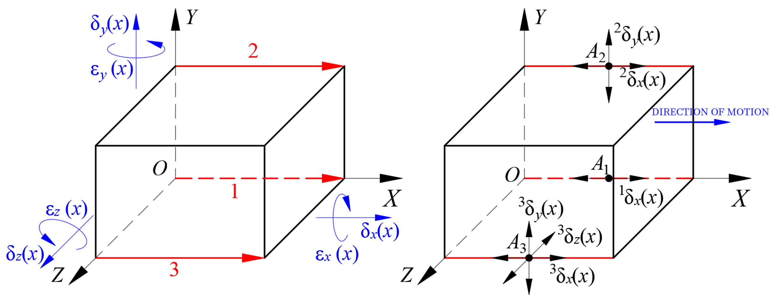
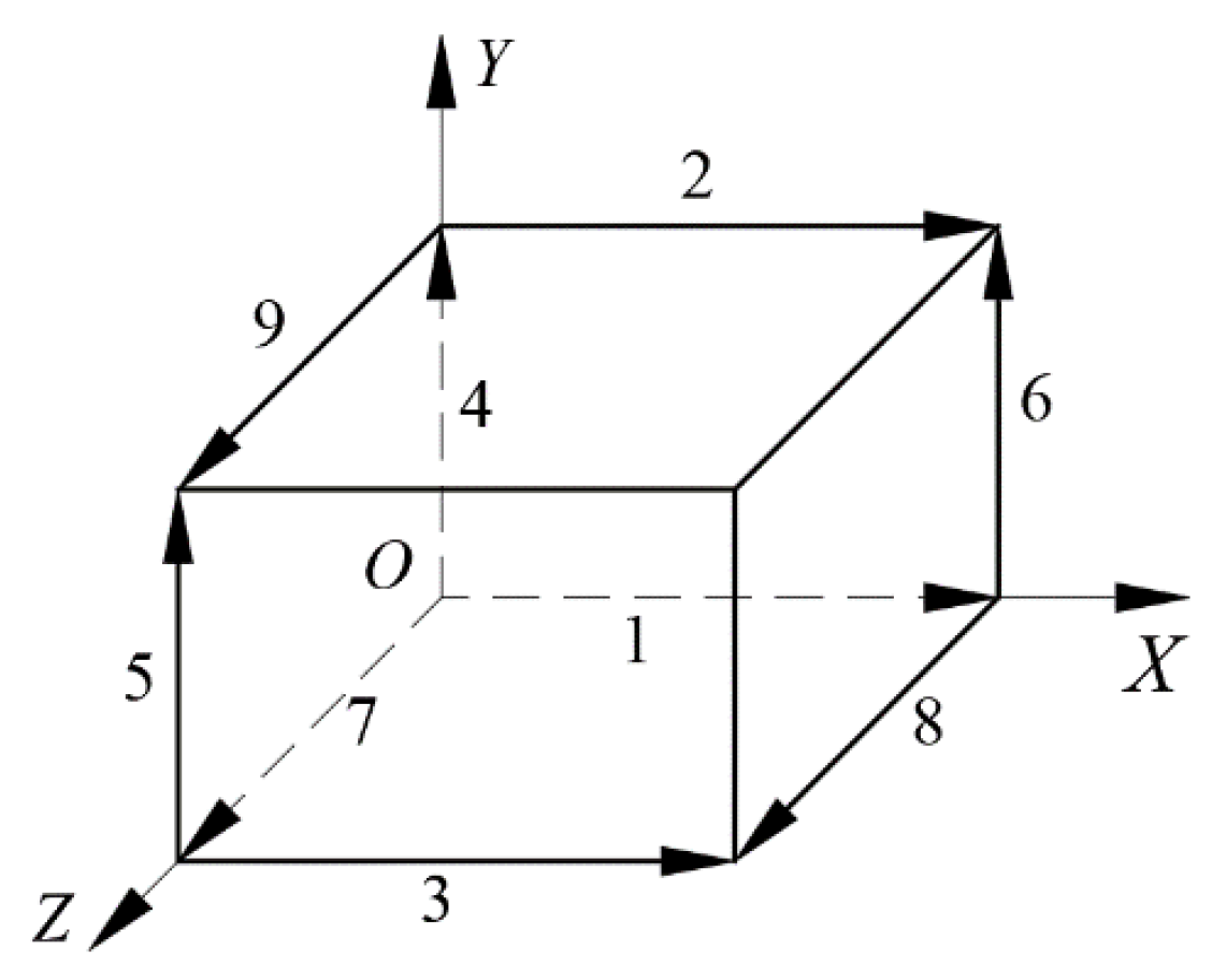
Based on the “nine-line method” of the machine tool linear feed axis error identification model, the principle is to use the laser interferometer to measure nine lines parallel to the three linear feed axes in the machine space through the identification algorithm to obtain all 21 linear feed axis geometric errors, as shown in Figure 1.

(1)

Identification principle of movement error and rotation error.

The identification of the three movement errors and three rotation errors of the linear feed axis is explained by taking the X-axis as an example.

As shown in Figure 2, a line parallel to the X-axis in the machine space $L_i\left(i=1,2,3\right)$ is selected and the point $A_i\left(x_i,y_i,z_i\right)$, i = 1, 2, 3 is taken on it.

When the point $A_1\left(x_1,y_1,z_1\right)$ moves along the X-axis at a distance of x, its positioning error along line 1 can be determined ${ }^1\delta x_{ }\left(x\right)$, at which point the chi-square transformation matrix of the error is

$$\mathit{E}\left(x\right)=\left[\begin{array}{cccc}1& -{\epsilon }_z\left(x\right)& {\epsilon }_y\left(x\right)& x+{\delta }_x\left(x\right)\\ {\epsilon }_z\left(x\right)& 1& -{\epsilon }_x\left(x\right)& {\delta }_y\left(x\right)\\ -{\epsilon }_y\left(x\right)& {\epsilon }_x\left(x\right)& 1& {\delta }_z\left(x\right)\\ 0& 0& 0& 1\end{array}\right]$$

(1)

Then, the motion error of the machine is

$$\left[\begin{array}{c}{ }^1\delta { }_x\left(x\right)\\ 0\\ 0\\ 0\end{array}\right]=\mathit{E}\left(x\right)\left[\begin{array}{c}{x}_1\\ y_1\\ z_1\\ 1\end{array}\right]-\left[\begin{array}{c}x+x_1\\ y_1\\ z_1\\ 1\end{array}\right]$$

(2)

collated from

$${ }^1\delta { }_x\left(x\right)={\delta }_x\left(x\right)-{\epsilon }_z\left(x\right)y_1+{\epsilon }_y\left(x\right)z_1$$

(3)

When the point $A_2\left(x_2,y_2,z_2\right)$ moves along the X-axis at a distance of x, its positioning error along line 2 can be measured ${ }^2\delta { }_x\left(x\right)$ while its straightness error along the Y-axis is measured ${ }^2{\delta }_y\left(x\right)$, at which time the machine motion error is

$$\left[\begin{array}{c}{ }^2\delta { }_x\left(x\right)\\ { }^2\delta { }_y\left(x\right)\\ 0\\ 0\end{array}\right]=\mathit{E}\left(x\right)\left[\begin{array}{c}{x}_2\\ y_2\\ z_2\\ 1\end{array}\right]-\left[\begin{array}{c}x+x_2\\ y_2\\ z_2\\ 1\end{array}\right]$$

(4)

collated from

$$\left\{\begin{array}{c}{ }^2{\delta }_x\left(x\right)={\delta }_x\left(x\right)-{\epsilon }_z\left(x\right)y_2+{\epsilon }_y\left(x\right)z_2\\ { }^2{\delta }_y\left(x\right)={\delta }_y\left(x\right)-{\epsilon }_x\left(x\right)z_2+{\epsilon }_z\left(x\right)x_2\end{array}\right.$$

(5)

When the point $A_3\left(x_3,y_3,z_3\right)$ moves along the X-axis at a distance of x, its positioning error along line 3 can be measured ${ }^3{\delta }_x\left(x\right)$ while its straightness error along the Y-axis ${ }^3{\delta }_y\left(x\right)$ and straightness error along the Z-axis ${ }^3{\delta }_z\left(x\right)$ are measured, at which time the machine motion error is

$$\left[\begin{array}{c}{ }^3{\delta }_x\left(x\right)\\ { }^3{\delta }_y\left(x\right)\\ { }^3{\delta }_z\left(x\right)\\ 0\end{array}\right]=\mathit{E}\left(x\right)\left[\begin{array}{c}{x}_3\\ y_3\\ z_3\\ 1\end{array}\right]-\left[\begin{array}{c}x+x_3\\ y_3\\ z_3\\ 1\end{array}\right]$$

(6)

collated from

$$\left\{\begin{array}{c}{ }^3{\delta }_x\left(x\right)={\delta }_x\left(x\right)-{\epsilon }_z\left(x\right)y_3+{\epsilon }_y\left(x\right)z_3\\ { }^3{\delta }_y\left(x\right)={\delta }_y\left(x\right)-{\epsilon }_x\left(x\right)z_3+{\epsilon }_z\left(x\right)x_3\\ { }^3{\delta }_z\left(x\right)={\delta }_z\left(x\right)-{\epsilon }_y\left(x\right)x_3+{\epsilon }_x\left(x\right)y_3\end{array}\right.$$

(7)

Combining Equations (3), (5), and (7), and expressing them in a matrix, we obtain

$$\left[\begin{array}{c}{ }^1{\delta }_x\left(x\right)\\ { }^2{\delta }_x\left(x\right)\\ { }^2{\delta }_y\left(x\right)\\ { }^3{\delta }_x\left(x\right)\\ { }^3{\delta }_y\left(x\right)\\ { }^3{\delta }_z\left(x\right)\end{array}\right]=\left[\begin{array}{cccccc}1& 0& 0& 0& z_1& -y_1\\ 1& 0& 0& 0& z_2& -y_2\\ 0& 1& 0& -z_2& 0& x_2\\ 1& 0& 0& 0& z_3& -y_3\\ 0& 1& 0& -z_3& 0& x_3\\ 0& 0& 1& y_3& -x_3& 0\end{array}\right]\left[\begin{array}{c}{\delta }_x\left(x\right)\\ {\delta }_y\left(x\right)\\ {\delta }_z\left(x\right)\\ {\epsilon }_x\left(x\right)\\ {\epsilon }_y\left(x\right)\\ {\epsilon }_z\left(x\right)\end{array}\right]$$

(8)

The order is as follows:

$\Delta \left(x\right)={\left[\begin{array}{cccccc}{ }^1{\delta }_x\left(x\right)& { }^2{\delta }_y\left(x\right)& { }^2{\delta }_y\left(x\right)& { }^3{\delta }_x\left(x\right)& { }^3{\delta }_y\left(x\right)& { }^3{\delta }_z\left(x\right)\end{array}\right]}^T$

$\mathit{e}\left(x\right)={\left[\begin{array}{cccccc}{\delta }_x\left(x\right)& {\delta }_y\left(x\right)& {\delta }_z\left(x\right)& {\epsilon }_x\left(x\right)& {\epsilon }_y\left(x\right)& {\epsilon }_z\left(x\right)\end{array}\right]}^T$

Then, there is

$$\Delta \left(x\right)=\mathit{A}\left(x\right)\mathit{e}\left(x\right)$$

(9)

Selecting the appropriate number of points on the line $L_i\left(i=1,2,3\right)$ such that the matrix $A\left(x\right)$ is full rank, there exists a unique solution to Equation (9).

$$\mathit{e}\left(x\right)=\mathit{A}{\left(x\right)}^{-1}\Delta \left(x\right)$$

(10)

The above Equation (10) is the geometric error identification model of the X-axis.

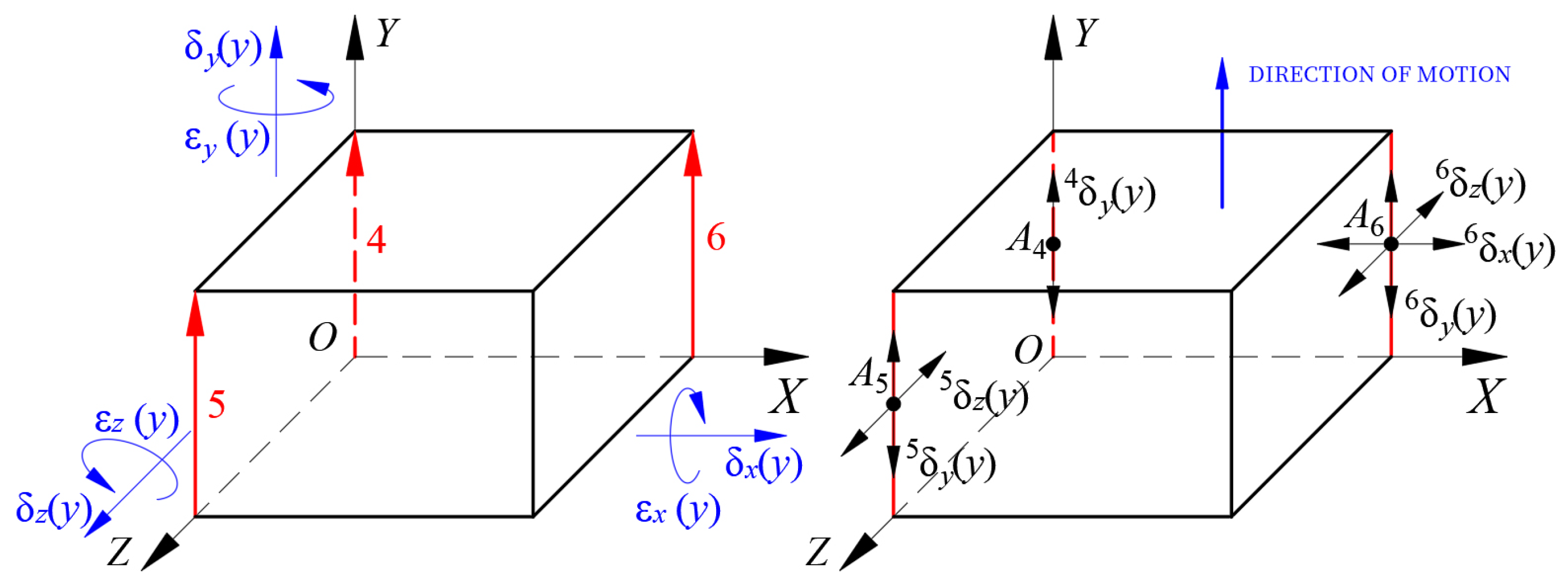
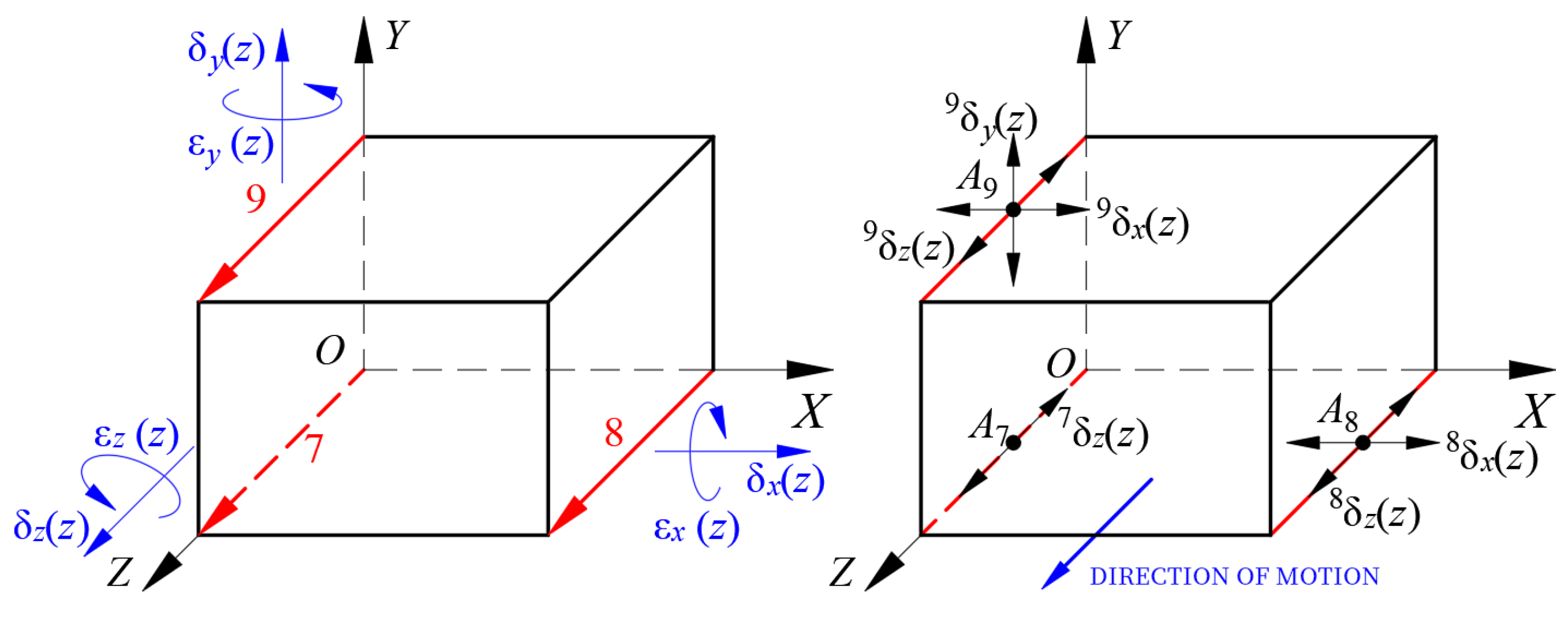
Similarly, according to Figure 3 and Figure 4, twelve other geometric errors generated by the Y-axis and Z-axis motions can be obtained: ${\delta }_x\left(y\right)$, ${\delta }_y\left(y\right)$, ${\delta }_z\left(y\right)$, ${\epsilon }_x\left(y\right)$, ${\epsilon }_y\left(y\right)$, ${\epsilon }_z\left(y\right)$ and ${\delta }_x\left(z\right)$, ${\delta }_y\left(z\right)$, ${\delta }_z\left(z\right)$, ${\epsilon }_x\left(z\right)$, ${\epsilon }_y\left(z\right)$, ${\epsilon }_z\left(z\right)$.

(2)

Principle of verticality error identification.

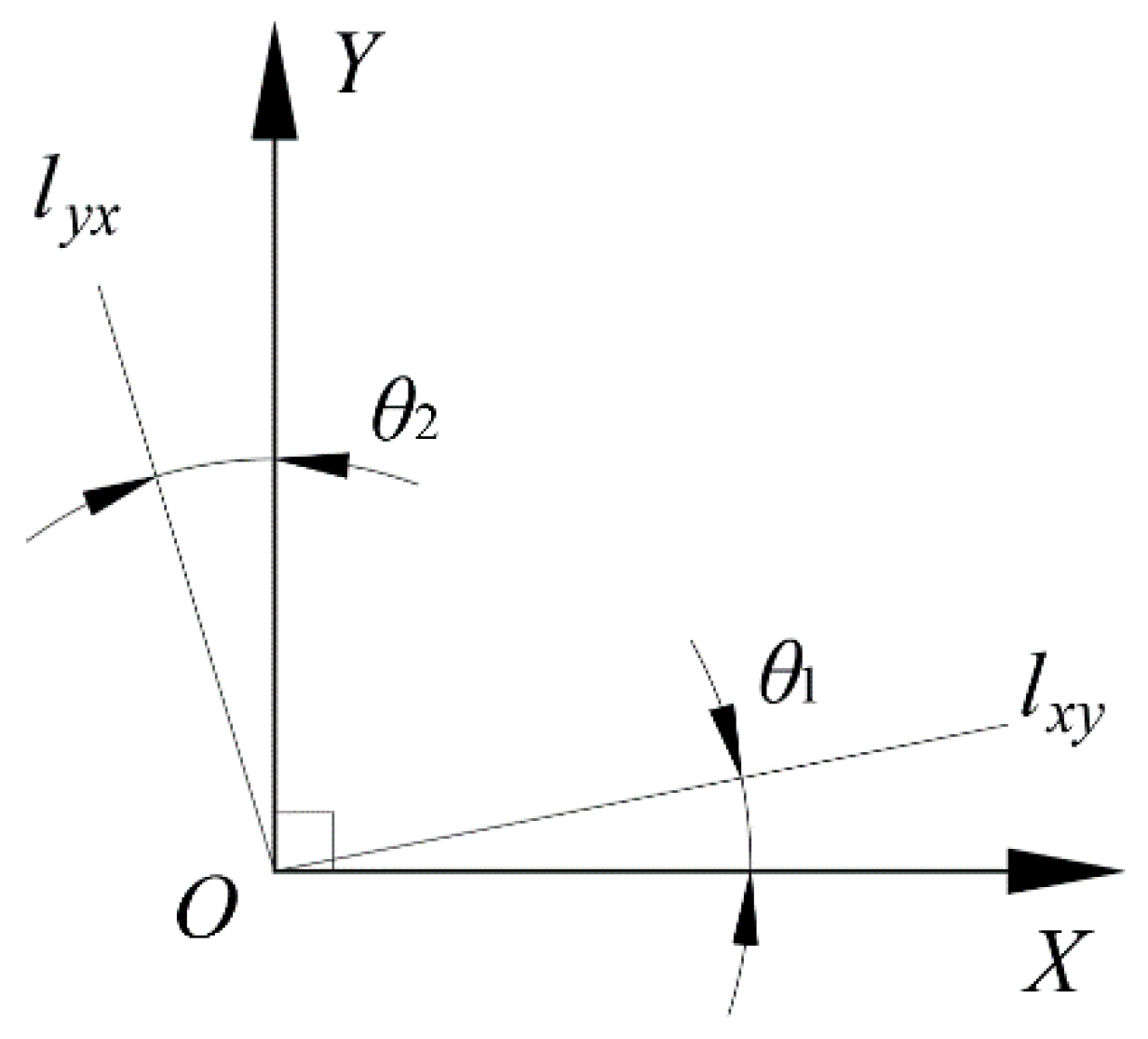
The calculation of the perpendicularity error between axes can be indirectly obtained by the above straightness error, and the perpendicularity error $S_{xy}$ of the X-axis and Y-axis is used as an example.

After the straightness errors ${\delta }_y\left(x\right)$ and ${\delta }_x\left(y\right)$ are obtained by the moving error identification principle, the values of ${\delta }_y\left(x\right)$ and ${\delta }_x\left(y\right)$ at each measurement point, ${\delta }_y\left(x_i\right)$ and ${\delta }_x\left(y_i\right)$, are fitted by the least squares method to obtain the fitted straightness error line $l_{xy}$ along the X-axis in the Y-direction and the fitted straightness error line $l_{yx}$ along the Y-axis in the X-direction, as shown in Figure 5. Where the angle between $l_{xy}$ and the X-axis is ${\theta }_1$, and the angle between $l_{yx}$ and the Y-axis is ${\theta }_2$. Then, the perpendicularity error between the X-axis and Y-axis is

$$S_{xy}={\theta }_2-{\theta }_1$$

(11)

Similarly, we can find the perpendicularity error between the X-axis and Z-axis, and the Y-axis and Z-axis with $S_{xz}$ and $S_{yz}$.

2.2. Principle of Identifying Geometric Errors of Machine Rotating Axes

The HMC-C100P machine in this paper (HMC-C100P, Shanghai, China) contains two rotary axes: A-axis and B-axis. The A-axis is the tool pendulum, and the B-axis is the rotary table. The geometric error identification of the B-axis motion is illustrated as an example.

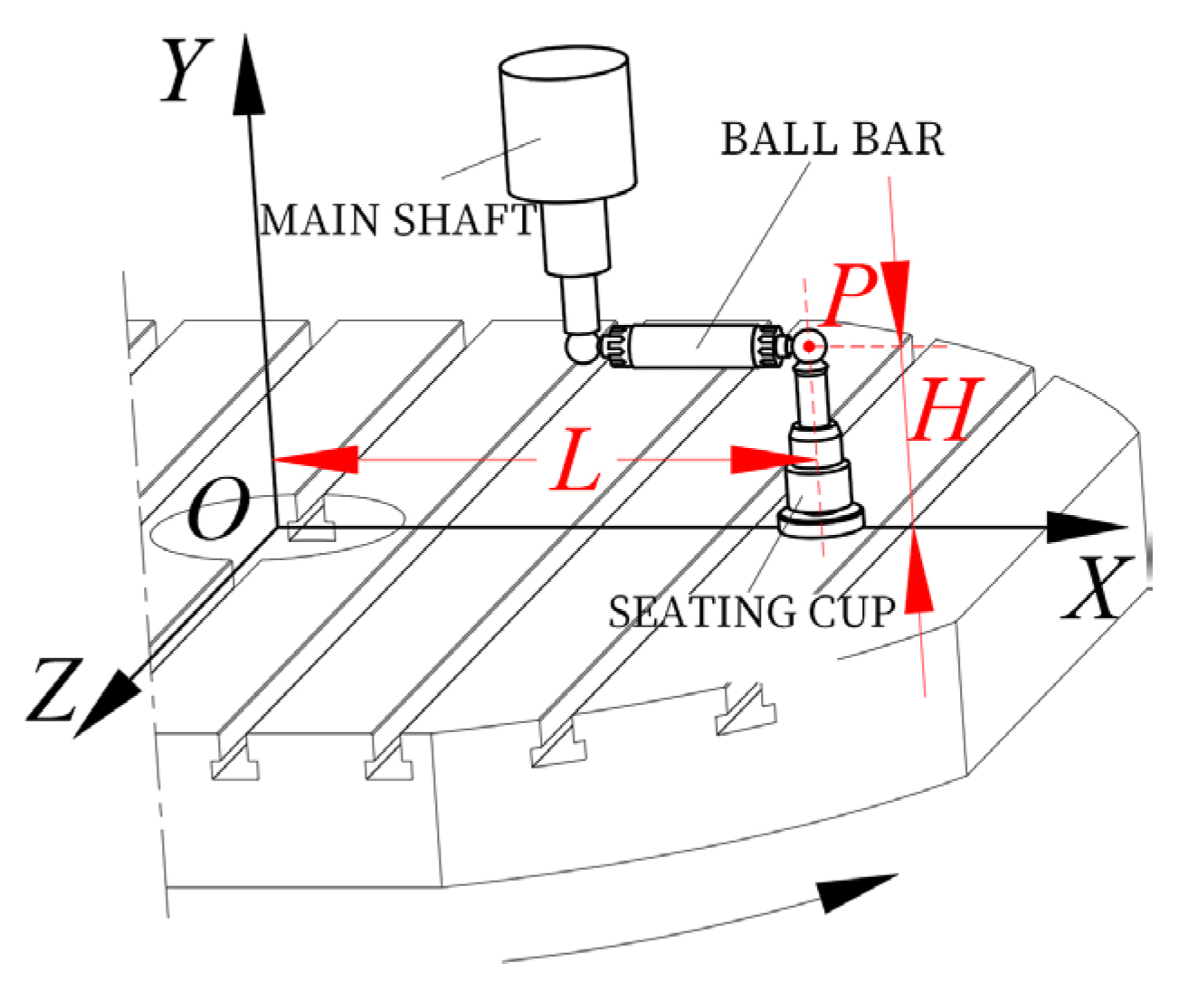
The B-axis movement will produce three movement errors along the X, Y, and Z axes, ${\delta }_x\left(B\right)$, ${\delta }_y\left(B\right)$, and ${\delta }_z\left(B\right)$, and three rotation errors around the X, Y, and Z axes, ${\epsilon }_x\left(B\right)$, ${\epsilon }_y\left(B\right)$, and ${\epsilon }_z\left(B\right)$. Establish the coordinate system as shown in Figure 6, and refer to the machine tool coordinate system for each axis direction. Fix the cup on the machine table and connect one end of the ballbar to the cup and the other end to the spindle. Assume that the distance between the center P of the ball at the end of the cup and the origin is L, and the distance from the table surface is H. The flush coordinates of the center P at the initial time can be expressed as $P={\left[\begin{array}{cccc}L& H& 0& 1\end{array}\right]}^T$.

When the B-axis rotary table is turned through the angle $\beta$, the coordinates of the sphere center P in the error-free motion state and the error-containing motion state, respectively, are

$$P_i=\left[\begin{array}{cccc}\cos \beta & 0& \sin \beta & 0\\ 0& 1& 0& 0\\ -\sin \beta & 0& \cos \beta & 0\\ 0& 0& 0& 1\end{array}\right]\left[\begin{array}{c}L\\ H\\ 0\\ 1\end{array}\right]=\left[\begin{array}{c}L·\cos \beta \\ H\\ -L·\sin \beta \\ 1\end{array}\right]$$

(12)

$$\begin{array}{l}{P}_e=\left[\begin{array}{cccc}1& -{\epsilon }_z\left(B\right)& {\epsilon }_y\left(B\right)& {\delta }_x\left(B\right)\\ {\epsilon }_z\left(B\right)& 1& -{\epsilon }_x\left(B\right)& {\delta }_y\left(B\right)\\ -{\epsilon }_y\left(B\right)& {\epsilon }_x\left(B\right)& 1& {\delta }_z\left(B\right)\\ 0& 0& 0& 1\end{array}\right]\left[\begin{array}{cccc}\cos \beta & 0& \sin \beta & 0\\ 0& 1& 0& 0\\ -\sin \beta & 0& \cos \beta & 0\\ 0& 0& 0& 1\end{array}\right]\left[\begin{array}{c}L\\ H\\ 0\\ 1\end{array}\right]\\ \hspace{1em}=\left[\begin{array}{c}L·\cos \beta -L·\sin \beta ·{\epsilon }_y\left(B\right)-H·{\epsilon }_z\left(B\right)+{\delta }_x\left(B\right)\\ L·\cos \beta ·{\epsilon }_z\left(B\right)+L·\sin \beta ·{\epsilon }_x\left(B\right)+H+{\delta }_y\left(B\right)\\ -L·\sin \beta -L·\cos \beta ·{\epsilon }_y\left(B\right)+H·{\epsilon }_x\left(B\right)+{\delta }_z\left(B\right)\\ 1\end{array}\right]\end{array}$$

(13)

Then, in the actual working condition, the coordinate change in the center P of the small ball at the end of the seat cup is

$$\Delta P=P_e-P_i=\left[\begin{array}{c}-L·\sin \beta ·{\epsilon }_y\left(B\right)-H·{\epsilon }_z\left(B\right)+{\delta }_x\left(B\right)\\ L·\cos \beta ·{\epsilon }_z\left(B\right)+L·\sin \beta ·{\epsilon }_x\left(B\right)+{\delta }_y\left(B\right)\\ H·{\epsilon }_x\left(B\right)-L·\cos \beta ·{\epsilon }_y\left(B\right)+{\delta }_z\left(B\right)\\ 0\end{array}\right]=\left[\begin{array}{c}\Delta P_x\\ \Delta P_y\\ \Delta P_z\\ 0\end{array}\right]$$

(14)

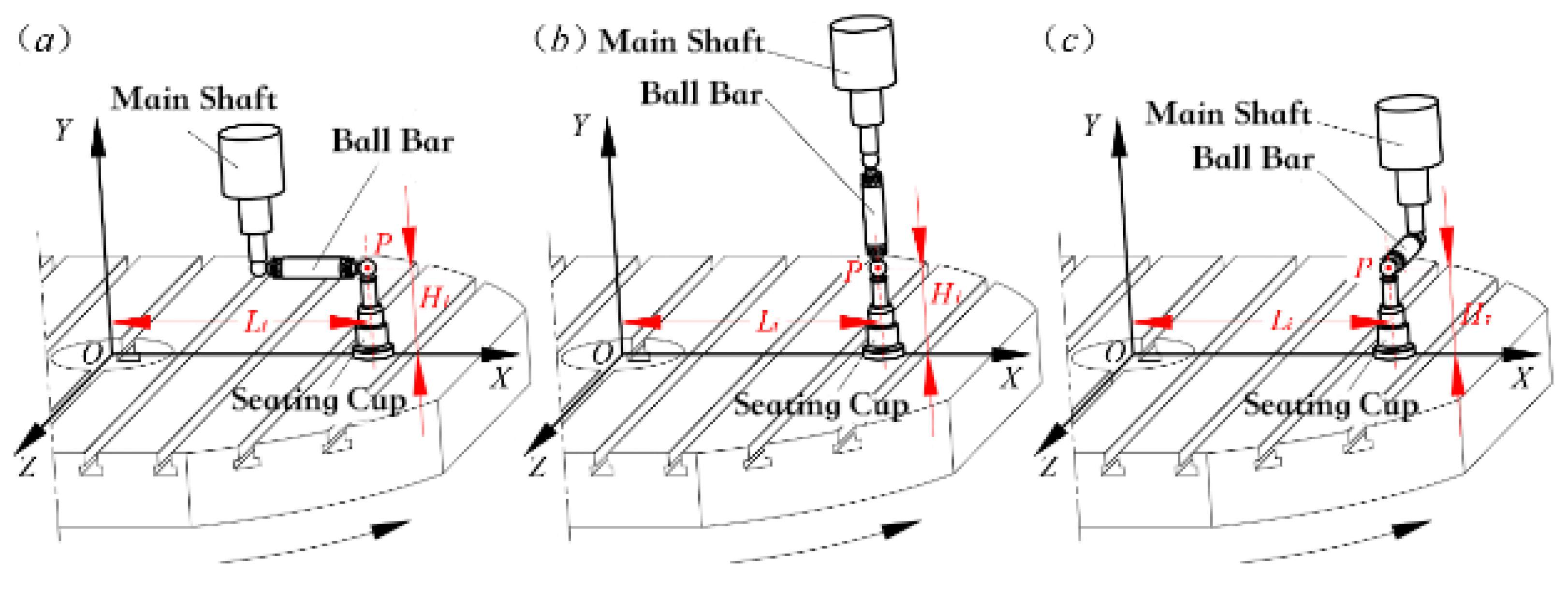
From Equation (13), the ballbar is installed at the same position (L, H) along the X, Y, and Z axes for three measurements to obtain the change in the spherical center P coordinate associated with the six basic geometric errors. However, at least six equations are needed to solve the six basic geometric errors, so the values of L and H need to be changed several times to identify the six basic geometric errors in the B-axis.

Table 1. Combination of positions for double ballbar installation.

Position	Combination Mode	Measurement Orientation
1	$(L_1,H_1)$	X, Y, Z
2	$(L_2,H_1)$	X, Y, Z
3	$(L_1,H_2)$	X, Y, Z

lists three different combinations of (L, H) for each position for each of the three axes, and the corresponding measurement patterns are shown in Figure 7.

According to Equation (13) and the measurement pattern shown in Figure 7, it is known that

$$\left\{\begin{array}{l}\Delta P_{x1,i}=-L_1·\sin {\beta }_i·{\epsilon }_{y,i}\left(B\right)-H_1·{\epsilon }_{z,i}\left(B\right)+{\delta }_{x,i}\left(B\right)\hfill \\ \Delta P_{y1,i}=L_1·\cos {\beta }_i·{\epsilon }_{z,i}\left(B\right)+L_1·\sin {\beta }_i·{\epsilon }_{x,i}\left(B\right)+{\delta }_{y,i}\left(B\right)\hfill \\ \Delta P_{z1,i}=H_1·{\epsilon }_{x,i}\left(B\right)-L_1·\cos {\beta }_i·{\epsilon }_{y,i}\left(B\right)+{\delta }_{z,i}\left(B\right)\hfill \\ \Delta P_{x2,i}=-L_2·\sin {\beta }_i·{\epsilon }_{y,i}\left(B\right)-H_1·{\epsilon }_{z,i}\left(B\right)+{\delta }_{x,i}\left(B\right)\hfill \\ \Delta P_{y2,i}=L_2·\cos {\beta }_i·{\epsilon }_{z,i}\left(B\right)+L_2·\sin {\beta }_i·{\epsilon }_{x,i}\left(B\right)+{\delta }_{y,i}\left(B\right)\hfill \\ \Delta P_{z2,i}=H_1·{\epsilon }_{x,i}\left(B\right)-L_2·\cos {\beta }_i·{\epsilon }_{y,i}\left(B\right)+{\delta }_{z,i}\left(B\right)\hfill \\ \Delta P_{x3,i}=-L_1·\sin {\beta }_i·{\epsilon }_{y,i}\left(B\right)-H_2·{\epsilon }_{z,i}\left(B\right)+{\delta }_{x,i}\left(B\right)\hfill \\ \Delta P_{y3,i}=L_1·\cos {\beta }_i·{\epsilon }_{z,i}\left(B\right)+L_1·\sin {\beta }_i·{\epsilon }_{x,i}\left(B\right)+{\delta }_{y,i}\left(B\right)\hfill \\ \Delta P_{z3,i}=H_2·{\epsilon }_{x,i}\left(B\right)-L_1·\cos {\beta }_i·{\epsilon }_{y,i}\left(B\right)+{\delta }_{z,i}\left(B\right)\hfill \end{array}\right.$$

(15)

The six errors of the B-axis can be identified by solving the above system of equations.

$${\delta }_{x,i}\left(B\right)=\Delta P_{x1,i}+L_1·\frac{\Delta P_{x1,i}-\Delta P_{x2,i}}{L_2-L_1}+H_1·\frac{\Delta P_{x1,i}-\Delta P_{x3,i}}{H_2-H_1}$$

(16)

$${\delta }_{y,i}\left(B\right)=\Delta P_{y1,i}-L_1·\frac{\Delta P_{y1,i}-\Delta P_{y2,i}}{L_1-L_2}$$

(17)

$${\delta }_{z,i}\left(B\right)=\Delta P_{z1,i}+L_1·\frac{\Delta P_{z1,i}-\Delta P_{z2,i}}{L_2-L_1}-H_1·\frac{\Delta P_{z1,i}-\Delta P_{z3,i}}{H_1-H_2}$$

(18)

$${\epsilon }_{x,i}\left(B\right)=\frac{\Delta P_{z1,i}-\Delta P_{z3,i}}{H_1-H_2}$$

(19)

$${\epsilon }_{y,i}\left(B\right)=\frac{\Delta P_{x1,i}-\Delta P_{x2,i}}{\left(L_2-L_1\right)·\sin {\beta }_i}$$

(20)

$${\epsilon }_{z,i}\left(B\right)=\frac{\Delta P_{x1,i}-\Delta P_{x3,i}}{H_2-H_1}$$

(21)

In Equations (16)–(21), the right subscript i indicates the number of equal parts of the B-axis slew stroke. It should be noted that since the measurements are taken at equal intervals within the slew stroke, the results obtained by the above identification model are the error dataset corresponding to the rotation angle ${\beta }_i$.

Similarly, the six geometric error elements generated by the A-axis tool pendulum head movement can be identified, and the rest are not repeated.

2.3. Principle of Workpiece Posture Error Identification

From the aforementioned analysis, it can be seen that there are six basic geometric errors in the machine space after clamping the workpiece—${\delta }_x\left(W\right)$, ${\delta }_y\left(W\right)$, ${\delta }_z\left(W\right)$, ${\epsilon }_x\left(W\right)$, ${\epsilon }_y\left(W\right)$, and ${\epsilon }_z\left(W\right)$—due to the geometric errors of the positioning elements of the fixture and the reference non-coincidence errors of the workpiece positioning surface. For the identification of these six basic geometric errors, this paper takes vise clamping as an illustrative example.

Figure 8 shows a schematic diagram of vise clamping, where the positioning surface limits one degree of freedom of movement of the workpiece $\overline{y}$ and two degrees of freedom of rotation $\stackrel{⌢}{x}$ and $\stackrel{⌢}{z}$; the thrust surface limits one degree of freedom of movement of the workpiece $\overline{x}$ and one degree of freedom of rotation $\stackrel{⌢}{y}$; the vise can produce a large clamping force after locking and friction between the thrust surface, clamping surface, and the workpiece, which together limit the freedom of movement of the workpiece along the Z-axis $\overline{z}$.

(1)

Identification of workpiece position error.

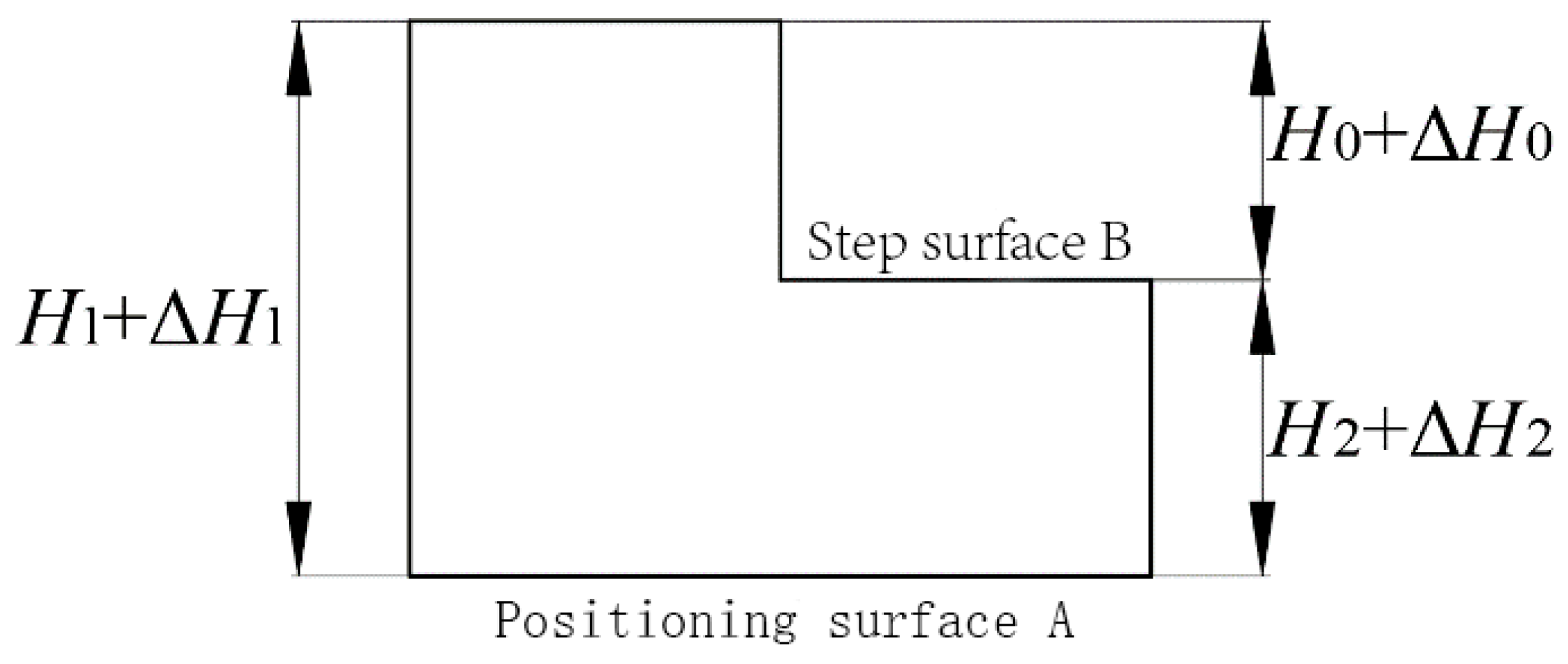
Take the height direction as an example. The workpiece dimension $H_1$ has been machined before clamping, the workpiece is positioned on the bottom surface A during clamping, and the dimension $H_2$ of the step surface B is machined directly. Then, the dimension $H_0$ to be machined is determined indirectly. The positioning date and the process date do not coincide, resulting in the movement error along the Y-axis ${\delta }_y\left(W\right)$, which can be solved by the process dimension chain shown in Figure 9.

From the relevant definition of the dimensional chain, it can be seen that the final dimension $H_0$ formed during the machining of the part is the closed ring, and the remaining dimensions $H_1$ and $H_2$ are the constituent rings, while the tolerance of the closed ring of the linear dimensional chain is equal to the sum of the tolerances of the constituent rings, namely

$$\Delta H_0=\Delta H_1+\Delta H_2$$

(22)

where $\Delta H_0$ is the tolerance of the closed ring $H_0$, and $\Delta H_1$ and $\Delta H_2$ are the tolerances of the constituent rings $H_1$ and $H_2$, respectively. Where $\Delta H_1$ has been determined cannot be changed, so we must improve the accuracy of the component ring $H_2$ to ensure the accuracy of the closed ring size $H_0$, and the reduced tolerance part is the reference non-coincidence error. Therefore, the Y-directional movement error of the workpiece in the machine space is identified as

$${\delta }_y\left(W\right)=\Delta H_2$$

(23)

Similarly, the X- and Z-directional movement errors of the workpiece in the machine space can be identified as follows:

$${\delta }_x\left(W\right)=\Delta L_2$$

(24)

$${\delta }_z\left(W\right)=\Delta W_2$$

(25)

where $\Delta H_2$, $\Delta L_2$, and $\Delta W_2$ are the tolerances of the workpiece in the height, length, and width directions, respectively.

(2)

Identification of workpiece attitude error.

The idea of identifying the workpiece attitude error is to measure the set of points on the positioning surface $\left(x_i,y_i,z_i\right)$, i = 1, 2, …, n, n ≥ 3, and use the least squares method to fit these scattered points to a plane. By calculating the angle between the fitted plane and the coordinate plane, the angular error of the workpiece in the machine space can be identified.

For the vise positioning surface, we have the manufacturing error of the thrust surface so that the workpiece in the machine space is around the X, Y, and Z axes of the rotation errors ${\epsilon }_x\left(W\right)$, ${\epsilon }_y\left(W\right)$, and ${\epsilon }_z\left(W\right)$. Let the general equation of the plane be

$$Ax+By+Cz+D=0$$

(26)

When $C\ne 0$, let ${\xi }_0=-\frac{A}{C}$, ${\xi }_1=-\frac{B}{C}$, and ${\xi }_2=-\frac{D}{C}$. Then, Equation (25) can be expressed as

$$z={\xi }_{0}x+{\xi }_{1}y+{\xi }_2$$

(27)

According to the principle of least squares, the distance of each measurement point from the least squares fitting plane should be minimized. $S={\displaystyle \sum _{i=1}^n{\left({\xi }_0{x}_i+{\xi }_1{y}_i+{\xi }_2-z_i\right)}^2}$ is minimal. Then, $\frac{\partial S}{\partial {\xi }_k}=0$, k = 0, 1, 2, should be satisfied. Thus, we have

$$\left[\begin{array}{ccc}{\displaystyle \sum _{i=1}^n{x}_i{ }^2}& {\displaystyle \sum _{i=1}^n{x}_i{y}_i}& {\displaystyle \sum _{i=1}^n{x}_i}\\ {\displaystyle \sum _{i=1}^n{x}_i{y}_i}& {\displaystyle \sum _{i=1}^n{y}_i{ }^2}& {\displaystyle \sum _{i=1}^n{y}_i}\\ {\displaystyle \sum _{i=1}^n{x}_i}& {\displaystyle \sum _{i=1}^n{y}_i}& 1\end{array}\right]\left[\begin{array}{c}{\xi }_0\\ {\xi }_1\\ {\xi }_2\end{array}\right]=\left[\begin{array}{c}{\displaystyle \sum _{i=1}^n{x}_i{z}_i}\\ {\displaystyle \sum _{i=1}^n{y}_i}{z}_i\\ {\displaystyle \sum _{i=1}^n{z}_i}\end{array}\right]$$

(28)

From the above Equation (28), the parameters ${\xi }_0$, ${\xi }_1$, and ${\xi }_2$ are obtained to obtain the equation of the positioning plane of the vise. The normal vector of the fitted plane is further obtained from Equation (27) as $\mathit{n}=\left({\xi }_0,{\xi }_1,-1\right)$.

To facilitate the calculation of the plane angle, directional restrictions are made on the equations of the fitted plane. As shown in Figure 10, let the fitted plane cross a certain coordinate axis (D = 0); the fitted positioning plane P₁ is perpendicular to the YOZ plane (A = 0), the fitted positioning plane P₂ is perpendicular to the XOY plane (C = 0), and the fitted stop plane P₃ is perpendicular to the XOZ plane (B = 0). Then, the equations of the fitted planes P₁, P₂, and P₃ are as follows

$$\left\{\begin{array}{c}{B}_{1}y+C_{1}z=0\\ A_{2}x+B_{2}y=0\\ A_{3}x+C_{3}z=0\end{array}\right.$$

(29)

Let $a_1=-\frac{B_1}{C_1}$, $b_0=-\frac{A_2}{B_2}$, and $c_0=-\frac{A_3}{C_3}$, and obtain the normal vectors of the fitted planes P₁, P₂, and P₃ as ${\mathit{n}}_1=\left(0,a_1,-1\right)$, ${\mathit{n}}_2=\left(b_0,-1,0\right)$, and ${\mathit{n}}_3=\left(c_0,0,-1\right)$, respectively. By calculating the angle between the normal vector of the fitted plane and the unit vector, the rotation error of the workpiece around the X, Y, and Z axes can be identified as

$$\left\{\begin{array}{l}{\epsilon }_x\left(W\right)=arc\cos 〈{\mathit{n}}_1,\mathit{j}〉\hfill \\ {\epsilon }_y\left(W\right)=arc\cos 〈{\mathit{n}}_3,\mathit{i}〉\hfill \\ {\epsilon }_z\left(W\right)=arc\cos 〈{\mathit{n}}_2,\mathit{j}〉\hfill \end{array}\right.$$

(30)

where i and j are the unit vectors along the X and Y axes.

3. Geometric Error Compensation Strategy

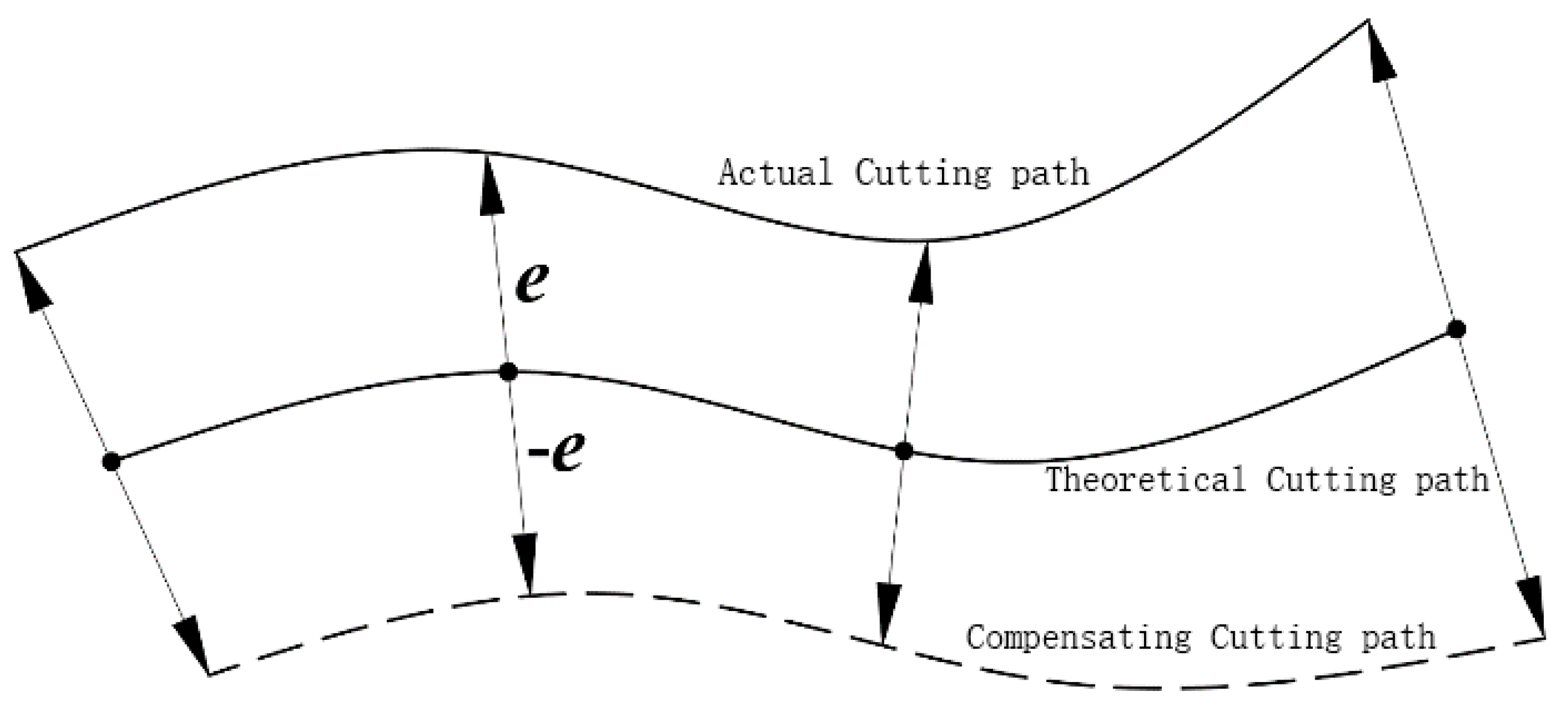
For the compensation of geometric errors, this paper adopts the error prediction and off-line compensation strategy. The idea is to indirectly derive the magnitude of each error value based on the instrument measurement data and the above identification principle on the basis of multi-source spatial error model prediction, and then make the actual tool position/tool axis vector relative to the theoretical tool position/tool axis vector to mirror the bias size error value to obtain the compensation tool position/tool axis vector to compensate the machining error by artificially creating a new error, as shown in Figure 11.

In the vertical and horizontal five-axis machining center, there is a motion coupling between the linear feed axis and the rotary axis. Even if the linear feed axis is stationary, only the rotary axis motion will bring about the displacement of the tool position point. Therefore, in the error compensation, the attitude compensation of the rotary axis is performed first, and then the position compensation of the linear feed axis is performed, and the specific algorithm is as follows [18].

(1)

Rotational axis attitude error compensation.

When the process system is moving without error in the ideal state, the ideal tool axis vector in the workpiece coordinate system at this time is obtained from Equation (3) to (17) as ${\mathit{V}}_i^W=\left[{}_{\mathit{Z}}{}^{\mathit{B}}\mathit{T}_{\mathit{i}}·{}_{\mathit{Y}}{}^{\mathit{A}}\mathit{T}_{\mathit{i}}\right]·{\mathit{V}}_{\mathit{i}}^{\mathit{T}}$, i.e.,

$$\left[\begin{array}{c}{v}_{xi}^W\\ v_{yi}^W\\ v_{zi}^W\\ 0\end{array}\right]=\left[\begin{array}{cccc}\cos {\beta }_i& 0& \sin {\beta }_i& 0\\ 0& 1& 0& 0\\ -\sin {\beta }_i& 0& \cos {\beta }_i& 0\\ 0& 0& 0& 1\end{array}\right]\left[\begin{array}{cccc}1& 0& 0& 0\\ 0& \cos {\alpha }_i& -\sin {\alpha }_i& 0\\ 0& \sin {\alpha }_i& \cos {\alpha }_i& 0\\ 0& 0& 0& 1\end{array}\right]\left[\begin{array}{c}0\\ 0\\ 1\\ 0\end{array}\right]=\left[\begin{array}{c}\sin {\beta }_i\cos {\alpha }_i\\ -\sin {\alpha }_i\\ \cos {\beta }_i\cos {\alpha }_i\\ 0\end{array}\right]$$

(31)

where $v_{xi}^W$, $v_{yi}^W$, and $v_{zi}^W$ denote the ideal attitude of the tool axis in the work coordinate system, and ${\alpha }_i$ and ${\beta }_i$ denote the machine turning angle in the ideal condition. Solve Equation (31) to obtain the machine turning angle under the ideal tool path trajectory as

$$\left\{\begin{array}{l}{\alpha }_i=\arcsin \left(-v_{yi}\right),0\le {\alpha }_i\le 2\pi \hfill \\ {\beta }_i=arctg\left(\frac{v_{xi}}{v_{zi}}\right),-\frac{\pi }{2}\le {\beta }_i\le \frac{\pi }{2}\hfill \end{array}\right.$$

(32)

Similarly, the actual machine turning angle when the process system is moving in the actual state with error is

$$\left\{\begin{array}{l}{\alpha }_r=\arcsin \left(-v_{yr}\right),0\le {\alpha }_r\le 2\pi \hfill \\ {\beta }_r=arctg\left(\frac{v_{xr}}{v_{zr}}\right),-\frac{\pi }{2}\le {\beta }_r\le \frac{\pi }{2}\hfill \end{array}\right.$$

(33)

where $v_{xr}^W$, $v_{yr}^W$, and $v_{zr}^W$ represent the actual attitudes of the tool axis in the work coordinate system. Then, the error compensation value can be expressed as $\Delta \alpha ={\alpha }_r-{\alpha }_i$, $\Delta \beta ={\beta }_r-{\beta }_i$, and the compensated machine turning angle by the reverse superposition compensation value is as follows:

$$\left\{\begin{array}{l}{\alpha }_c={\alpha }_i-\Delta \alpha =2{\alpha }_i-{\alpha }_r\hfill \\ {\beta }_c={\beta }_i-\Delta \beta =2{\beta }_i-{\beta }_r\hfill \end{array}\right.$$

(34)

(2)

Linear feed axis position error compensation.

When the process system moves without error in the ideal state, the position change in the tool position point is synchronized with the motion of the linear feed axis of the machine tool, and the ideal tool position point in the workpiece coordinate system is

$${\mathit{P}}_i^W=\left[\begin{array}{c}{p}_{xi}^W\\ p_{yi}^W\\ p_{zi}^W\\ 1\end{array}\right]=\left[\begin{array}{c}{x}_i\cos {\beta }_i+z_i\sin {\beta }_i+L\cos {\alpha }_i\sin {\beta }_i\\ y_i-L\sin {\alpha }_i\\ z_i\cos {\beta }_i-x_i\sin {\beta }_i+L\cos {\alpha }_i\cos {\beta }_i\\ 1\end{array}\right]$$

(35)

where $p_{xi}^W$, $p_{yi}^W$, and $p_{zi}^W$ denote the ideal positions of the tool position in the work coordinate system; $x_i$, $y_i$, and $z_i$ denote the motions of the machine tool linear feed axis in the ideal state; ${\alpha }_i$, ${\beta }_i$ denotes the machine tool turning angle in the ideal state; and L is the tool length. From Equation (35), obtaining the ideal tool path trajectory under the machine tool motion position is completed as follows:

$$\left\{\begin{array}{l}{x}_i=p_{xi}^W\cos {\beta }_i-p_{zi}^W\sin {\beta }_i\hfill \\ y_i=p_{yi}^W+L\sin {\alpha }_i\hfill \\ z_i=p_{xi}^W\sin {\beta }_i+p_{zi}^W\cos {\beta }_i-L\cos {\alpha }_i\hfill \end{array}\right.$$

(36)

Similarly, the actual motion position of the machine when the process system is in the actual state with error motion is

$$\left\{\begin{array}{l}{x}_r=p_{xr}^W\cos {\beta }_c-p_{zr}^W\sin {\beta }_c\hfill \\ y_r=p_{yr}^W+L\sin {\alpha }_c\hfill \\ z_r=p_{xr}^W\sin {\beta }_c+p_{zr}^W\cos {\beta }_c-L\cos {\alpha }_c\hfill \end{array}\right.$$

(37)

where $p_{xr}^W$, $p_{yr}^W$, and $p_{zr}^W$ represent the actual positions of the tool position in the workpiece coordinate system; it should be noted that in calculating the actual motion position of the machine, the machine tool angle ${\alpha }_c$, ${\beta }_c$ after the compensation of Equation (34) should be brought into the solution. Then, the machine tool linear feed axis error compensation values for $\Delta x=x_r-x_i$, $\Delta y=y_r-y_i$, and $\Delta z=z_r-z_i$, through the reverse superposition of compensation values to the compensated machine tool position, are found.

$$\left\{\begin{array}{l}{x}_c=x_i-\Delta x=2x_i-x_r\hfill \\ y_c=y_i-\Delta y=2y_i-y_r\hfill \\ z_c=z_i-\Delta z=2z_i-z_r\hfill \end{array}\right.$$

(38)

Finally, replace the X, Y, Z, A, and B values in the original NC code with the compensated machine positions $x_c$, $y_c$, and $z_c$, and machine angles ${\alpha }_c$ and ${\beta }_c$, to obtain the compensated NC code.

4. Example of Process System Error Measurement and Identification

4.1. Laser Interferometer-Based Measurement and Identification of Linear Axis Errors in Machine Tools

The equipment and instruments used in this experiment mainly include those described below.

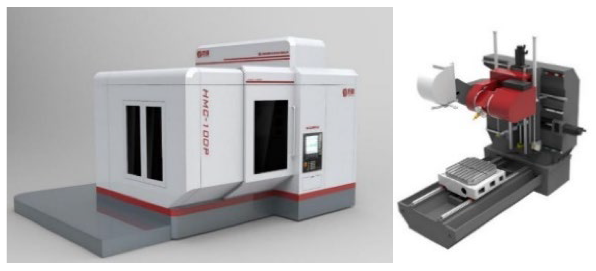
1. Five-axis machine tool: The vertical and horizontal conversion five-axis machining center is shown in Figure 12 (model HMC-C100P). The main technical parameters are detailed in

Table 2. Specification of vertical and horizontal 5-axis machining center.

Projects	Aluminum Machine Tools
Table turning radius	500 mm
Itinerary	X: 1190 mm
	Y: 1020 mm
	Z: 1250 mm
Spindle swing angle	A-axis −120°~+60°
	B-axis n × 360°
Maximum speed	24,000 r/min

.

2. Laser interferometer system: The XL-80 laser head has a laser frequency stabilization accuracy of ±0.05 ppm, a resolution of 1 nm, and a built-in USB communication interface. The maximum permissible acquisition movement speed of the whole laser interferometer system is 4 m/s, and the dynamic acquisition frequency is between 10 Hz and 50 kHz.

In order to ensure that the number of measurement points on each axis is the same, this experiment selects 800 mm of travel on each linear feed axis and sets the measurement points and automatic data acquisition according to Figure 13: 50 mm distance between measurement points, 4 s stop at each measurement point for data acquisition, and 4 mm head and tail overtravel.

As can be seen from Figure 13, the nine-line method requires nine measurements in the machine space parallel to the X, Y, and Z axes, respectively, and the coordinates of the starting and ending points of each line are shown in

Table 3. Coordinates of the starting and ending points of the measured lines.

Line	Starting Point	End Point	Line	Starting Point	End Point	Line	Starting Point	End Point
1	(0,0,0)	(800,0,0)	4	(0,0,0)	(0,800,0)	7	(0,0,0)	(0,0,800)
2	(0,800,0)	(800,800,0)	5	(0,0,800)	(0,800,800)	8	(800,0,0)	(800,0,800)
3	(0,0,800)	(800,0,800)	6	(800,0,0)	(800,800,0)	9	(0,800,0)	(0,800,800)

. Figure 14 shows the experimental site for geometric error detection. In order to reduce the measurement of accidental errors, each measurement line is measured six times reciprocally, and then the average value of the measurements is taken for geometric error element identification.

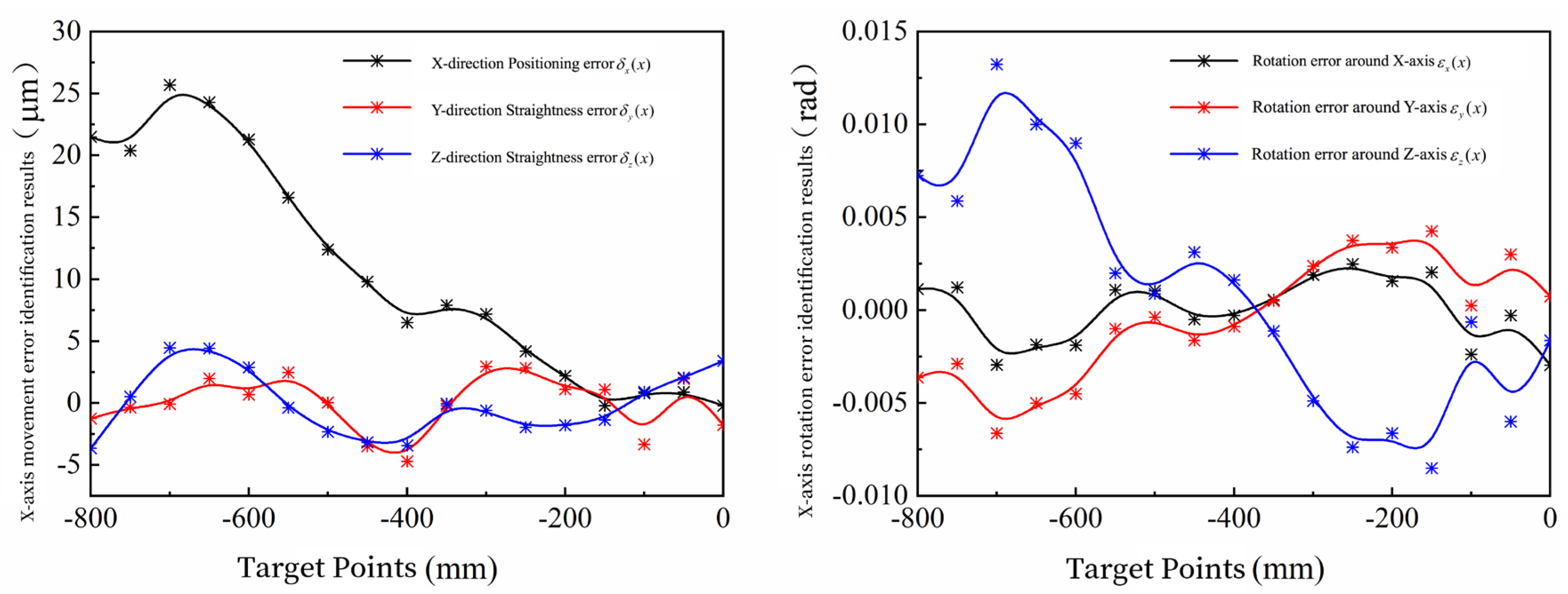
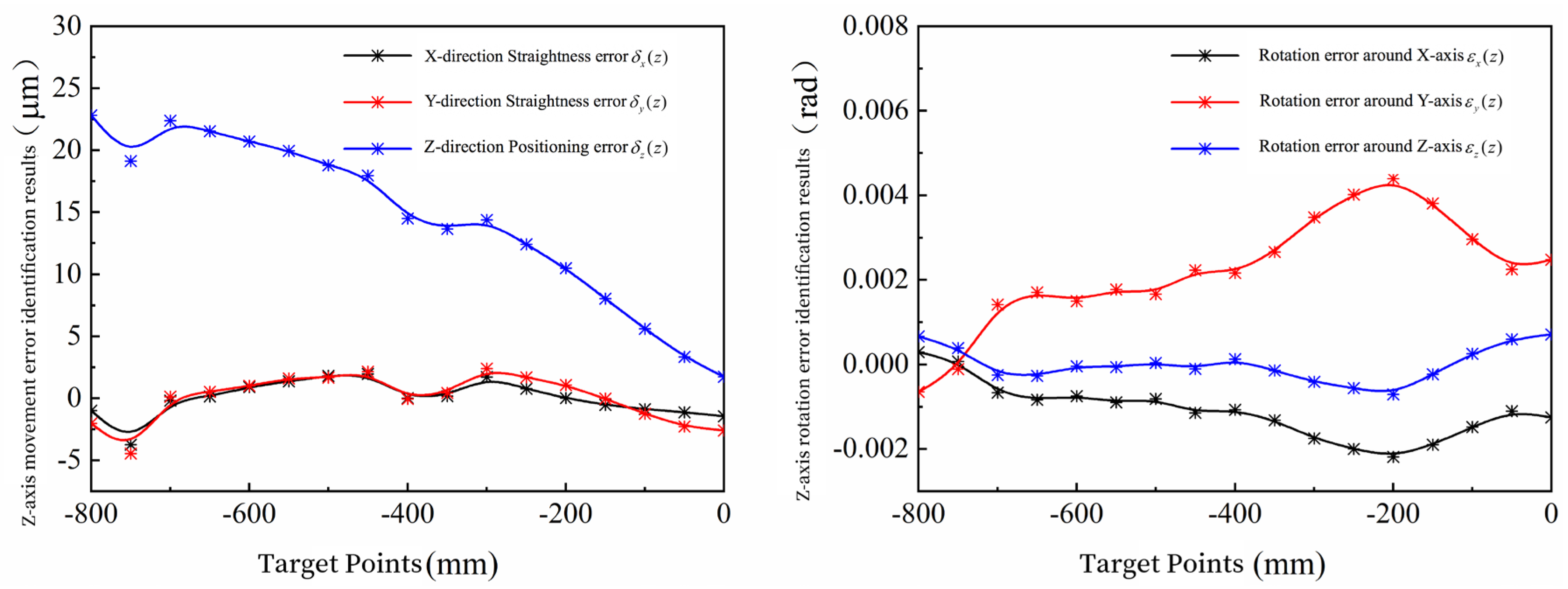
Since the geometric error measurements of the linear feed axes are linear in length, the positioning errors in the moving errors ${\delta }_x\left(x\right)$, ${\delta }_y\left(y\right)$, and ${\delta }_z\left(z\right)$ can be identified by taking the experimental data for lines 1, 4, and 7. The Renishaw Laser XL data analysis software is based on a least squares fit to a straightness baseline, so here the straightness error for each axis is expressed as the residual from each measurement point to the least squares fitted line. The simple processed measurement data are substituted into Equation (10), and the error identification results of the three linear feed axes are calculated by MATLAB R2018a, as shown in Figure 15, Figure 16 and Figure 17. According to the identification principle of Equation (11), the three perpendicularity errors can be obtained from the difference of the angle between the fitted line and the horizontal axis, and the results are shown in

Table 4. Verticality error identification results.

Error Symbol	Sxy/10−5 rad	Sxz/10−5 rad	Syz/10−5 rad
Identification Results	0.472	0.292	0.133

.

4.2. Ballbar-Based Measurement and Identification of Machine Tool Rotary Axis Errors

This section is based on the Renishaw QC20-W ballbar and checks the A and B axes of rotation errors of machine tools. The equipment and instruments used in this experiment include the following:

• Five-axis machine tool: Model and performance parameters are described in Section 4.1.
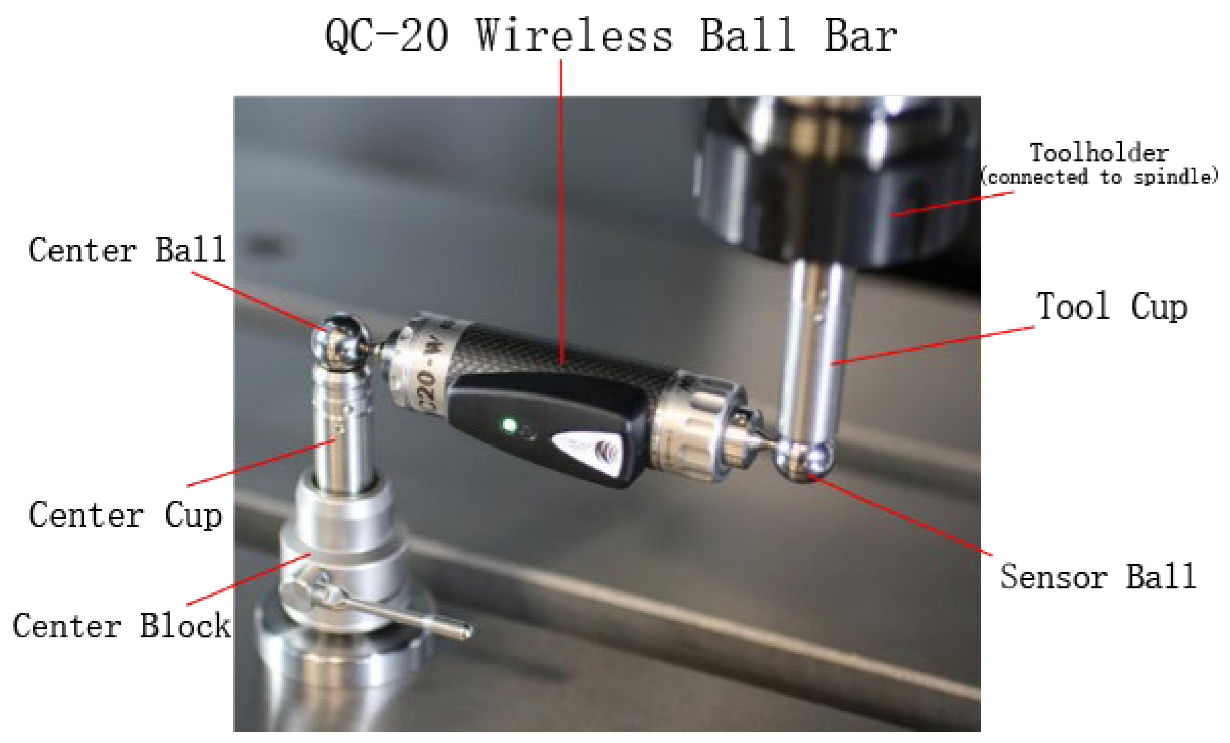
• Ballbar system: As shown in Figure 18, QC20-W contains a high-precision telescopic linear sensor inside, and the parameters are shown in

  Table 5. Double ballbar system specifications.

  Projects	Parameters	Projects	Parameters
  Sensor resolution	0.1 µm	Sensor resolution	1000 Hz
  Ballbar measurement accuracy	±(0.7 + 0.3% L) µm	Ballbar measurement accuracy	Bluetooth II
  Ballbar measurement range	±1.0 mm	Ballbar measurement range	10 m Typical
  Sensor stroke	−1.25 mm~+1.75 mm	Sensor stroke	0 °C~40 °C

  . There is a precision sphere at each end of the ballbar; one end is connected to the table and one end is connected to the spindle.

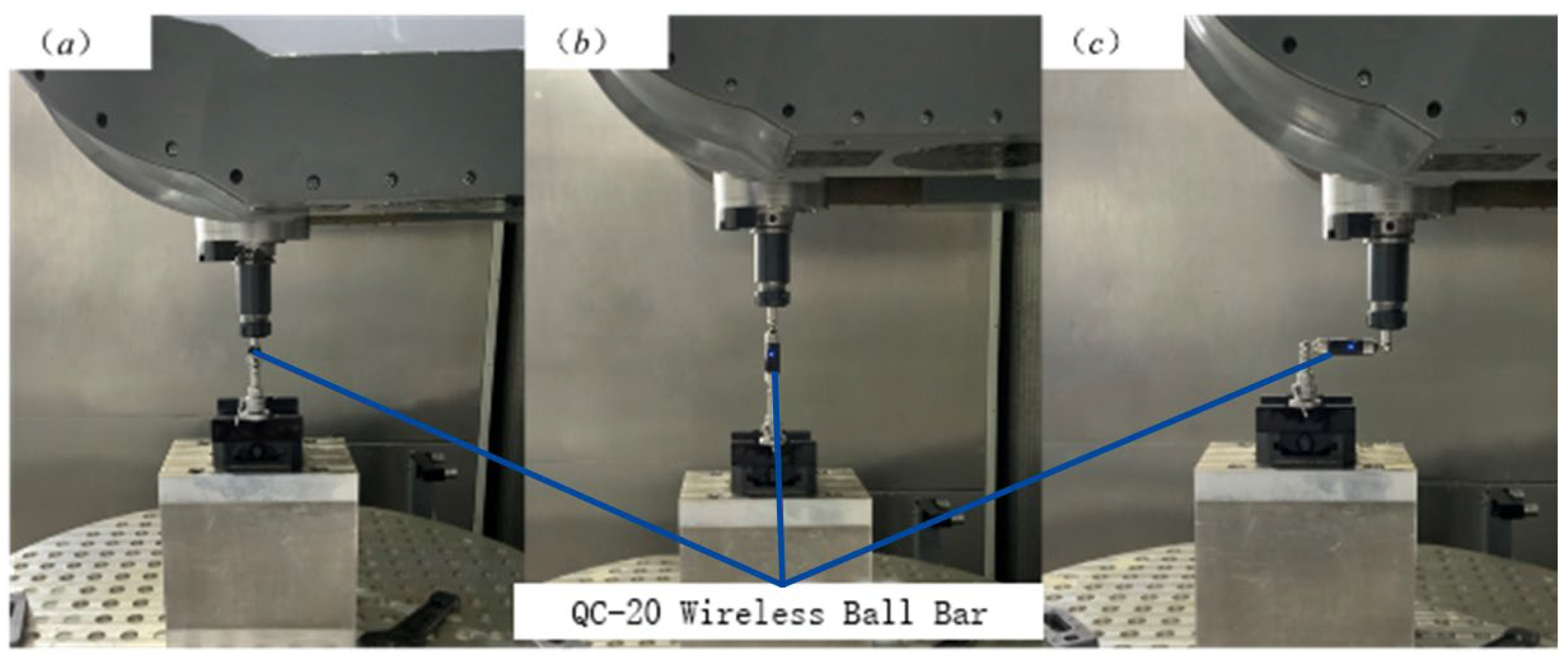
Figure 19 shows the experimental site of the B-axis rotary table geometry error detection. The standard rod length of the ballbar used in this experiment is 100 mm, and the measurement range of the B-axis rotary table is 0°~360°, with a measurement spacing of 10°, a 10° head-to-tail crossing, and a 5 s pause at each measurement position for reading. The distance combination of the ballbar installation is shown in

Table 6. Combination of distances for double ballbar mounting on rotary axis.

Measurement Orientation/mm	X, Y, Z	X, Y, Z	X, Y, Z
Position $(L_A,H_A)$	(45.966,152.050)	(45.966,185.746)	(89.358,185.746)
Position $(L_B,H_B)$	(40.043,73.720)	(60.843,73.720)	(60.843,128.720)

: position $\left(L_B,H_B\right)$. Three measurements are taken in the X, Y, and Z directions at the same position and the amount of rod length change is recorded.

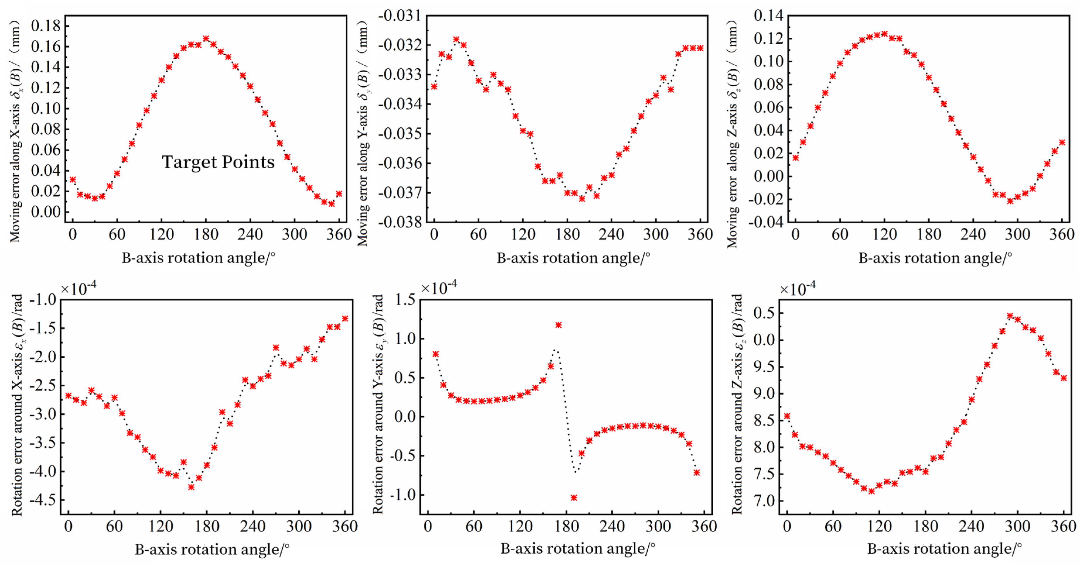
The geometric error identification results of the B-axis rotary table are calculated by MATLAB by substituting the processed measurement data into Equations (16)–(21). Here, the identification result is the error dataset corresponding to the rotation angle of the B-axis ${\beta }_i$, as shown in Figure 20.

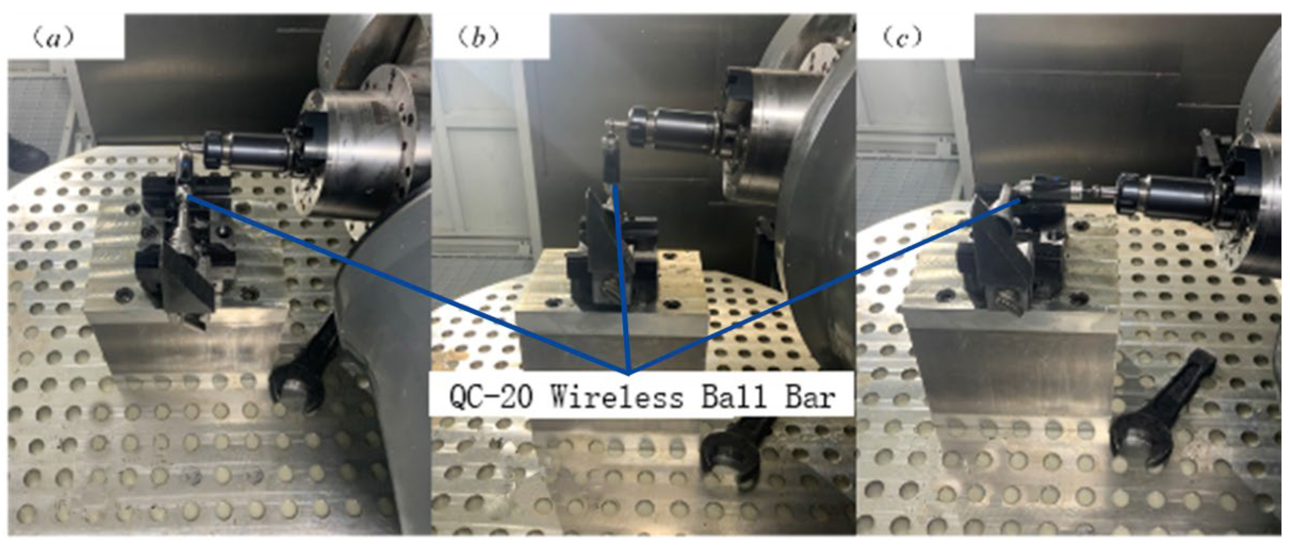
Similarly, the A-axis tool pendulum head was tested, and the experimental site of A-axis geometric error detection is shown in Figure 21. The measurement range of the A-axis tool pendulum head was 0°~−90°, the measurement distance was 5°, the first and last transitions were 5°, and the pause was 5 s at each measurement position for reading. The distance combination of the ballbar installation is shown in Table 6: position $\left(L_A,H_A\right)$. Three measurements in the X, Y, and Z directions were taken at the same position and the amount of rod length change was recorded.

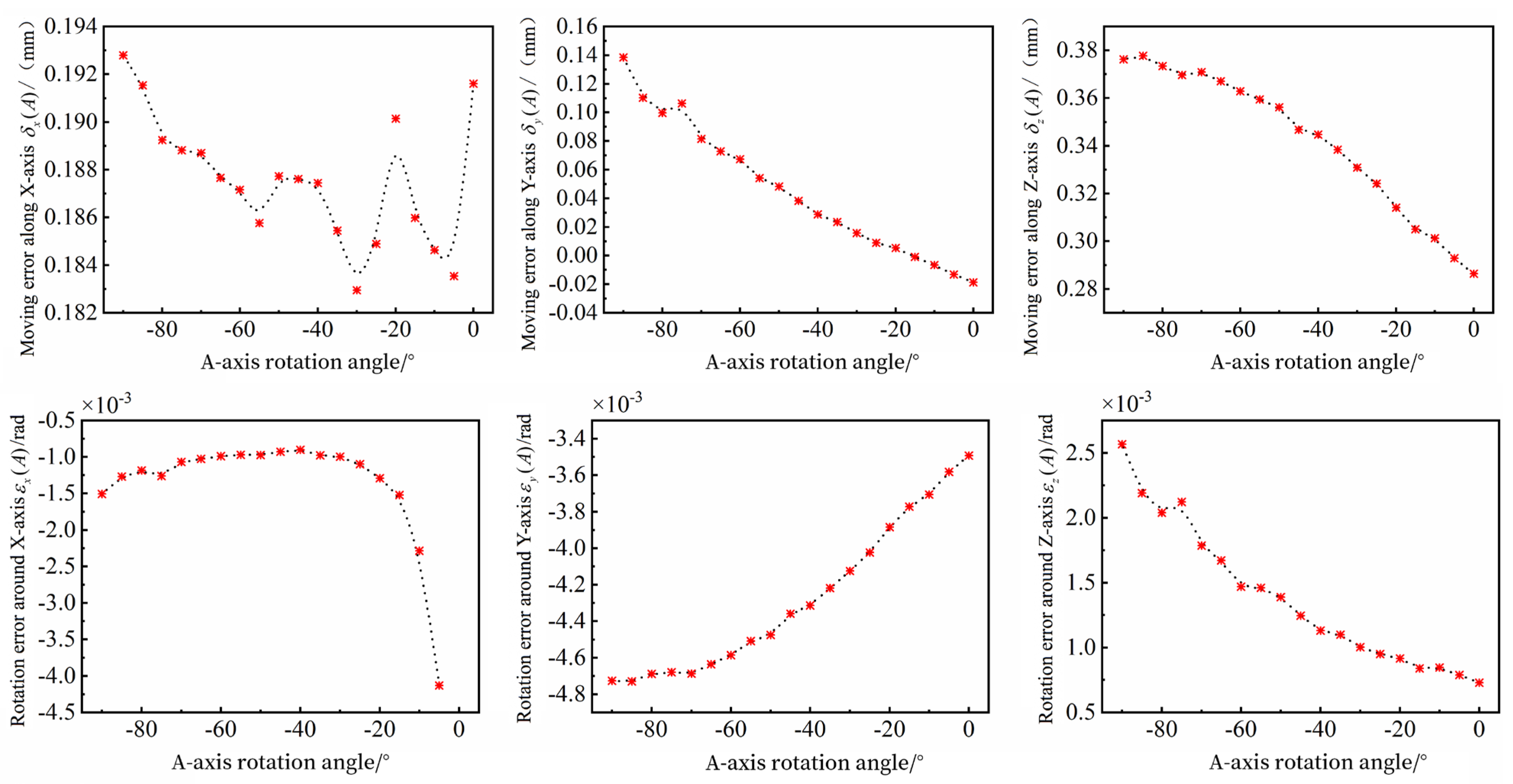
The geometric error identification results of the A-axis tool pendulum are obtained by substituting the processed measurement data into Equations (22)–(27) and calculating them through MATLAB. Here, the identification result is the error dataset corresponding to the rotation angle of the A-axis ${\alpha }_i$, as shown in Figure 22.

4.3. Measurement and Identification of Workpiece Posture Errors Based on Contact Probes

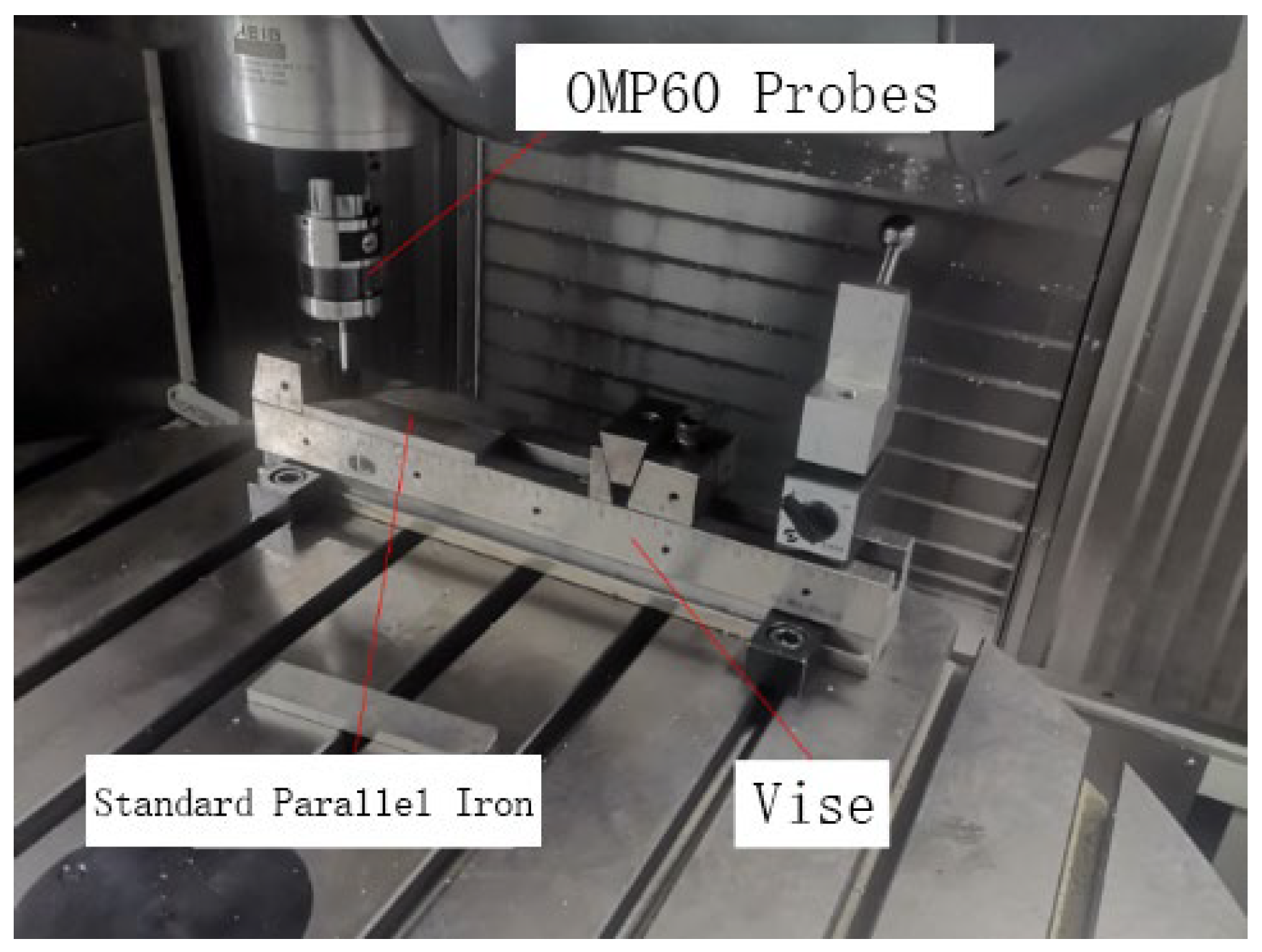
This subsection conducts an experiment on workpiece attitude error identification, as shown in Figure 23, for the workpiece attitude error measurement site. The main instruments used in the experiment are the Renishaw OMP60 probe, a vise, and a standard parallel iron.

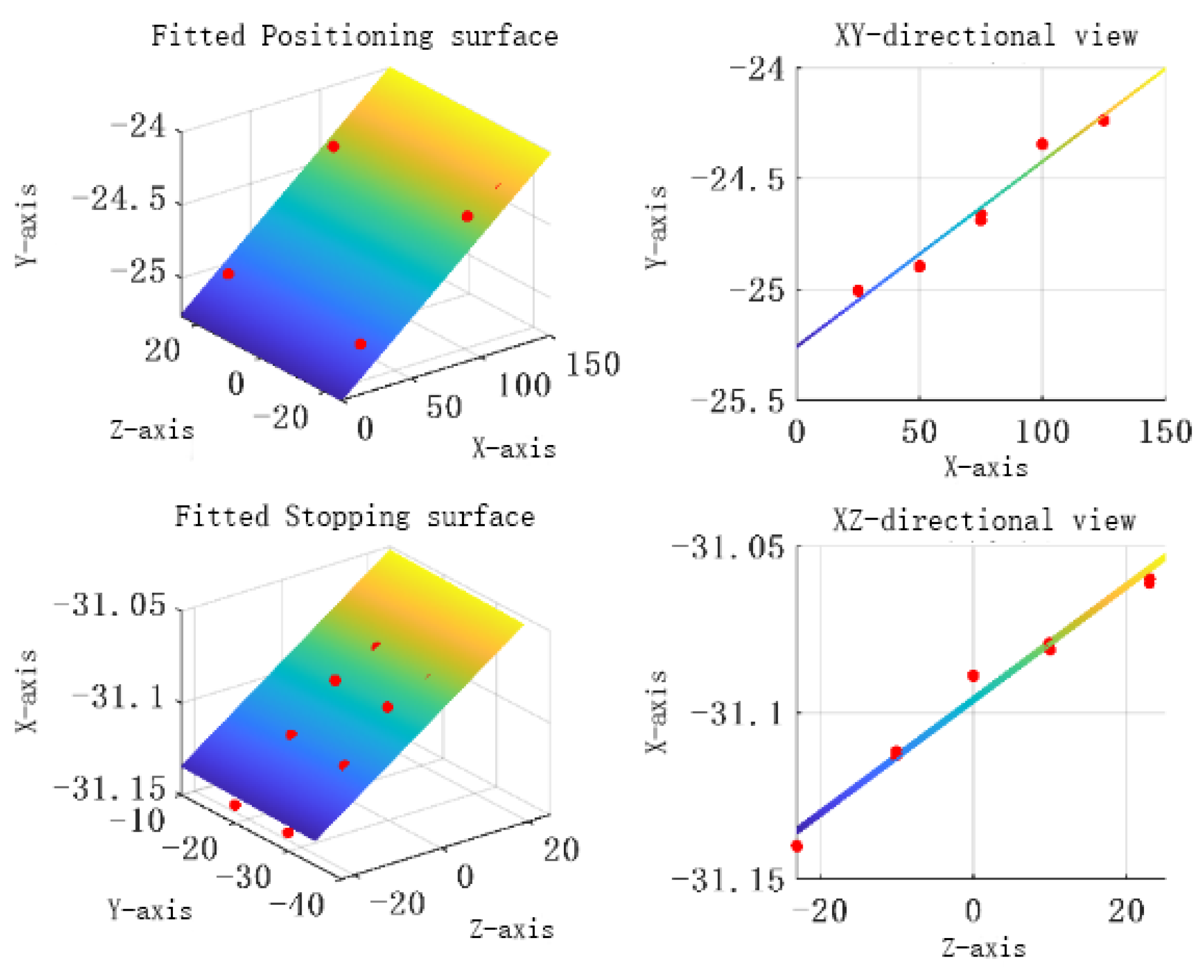
The measured point data are shown in

Table 7. Data points for measurement of workpiece positioning surface and thrust surface.

Positioning Surface/mm			Thrust Surface/mm
X	Y	Z	X	Y	Z
25.051	−25.008	−20.093	−23.010	−20.002	−31.140
25.010	−25.003	21.215	−23.056	−30.011	−34.140
50.092	−24.892	20.786	−10.060	−20.046	−31.112
50.038	−24.899	−21.045	−10.093	−30.082	−31.113
75.032	−24.689	−21.438	−0.007	−20.092	−31.089
75.018	−24.660	21.300	−0.001	−29.908	−31.089
100.079	−24.347	20.909	9.911	−19.929	−31.079
100.090	−24.343	−20.903	9.990	−29.923	−31.081
125.077	−24.235	−20.588	22.999	−19.931	−31.060
125.101	−24.239	20.351	22.975	−29.928	−31.061

. The data points are fitted with least squares to obtain the actual positioning surface and the stopping surface, and the results are shown in Figure 24. The angle between the normal vector of the fitted plane and the normal vector of the coordinate plane is further calculated to obtain the workpiece attitude errors of ${\epsilon }_x\left(W\right)=0.0084$ rad, ${\epsilon }_y\left(W\right)=0.0017$ rad, and ${\epsilon }_z\left(W\right)=0.0084$ rad.

As mentioned in the identification principle in Section 2.3 above, the position error of the workpiece can be expressed by the dimensional tolerances in three directions. According to the international standard ISO 10797:2020, the dimensional tolerance of the S-shaped specimen other than the flatness of the bottom surface is ±0.1 mm [19], so the position error of the workpiece is ${\delta }_x\left(W\right)={\delta }_y\left(W\right)={\delta }_z\left(W\right)=0.1$ mm.

4.4. Machining Verification of S-Shaped Specimen-Based Compensation Strategy

In order to verify the feasibility of the compensation method in this paper, this subsection carries out the verification of the compensation strategy based on the S-shaped specimen. The main equipment used in the experiment included the following:

• One set of HMC-C100P five-axis machines.
• Hexagon bridge-type CMM, one set.

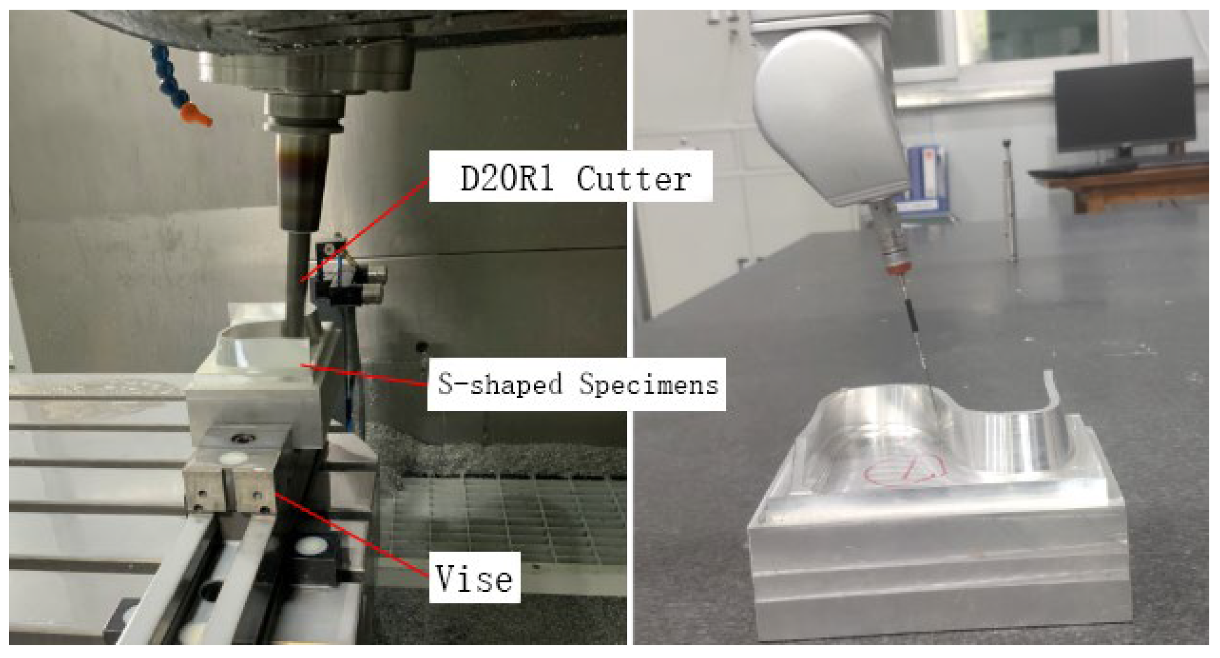
The processing and measurement site of the S-shaped specimen is shown in Figure 25. Due to the limited experimental materials, the size of the “S-shaped specimen” used in this experiment was proportionally reduced by two on the basis of the standard part. The thickness of the stretched edge strip was 8 mm, the height was 25 mm, and the material of the specimen was 7050-T7451 aluminum alloy. The tool used for the experiment was a carbide end mill with a diameter of 20 mm and a tip filet of 1 mm. The experimental machining parameters are shown in

Table 8. Processing parameters of S-shaped specimens.

Spindle Speed	Roughing Feed per Tooth	Finishing Feed per Tooth	Depth of Cut	Roughing Cut Width	Finishing Cut Width
8000 r/min	0.25 mm	0.15 mm	3 mm	1 mm	0.1 mm

.

4.4.1. Assessment of Measurement Uncertainty

• Calculation of uncertainty components.

(1) Uncertainty components due to CMM oscillometric errors $u_E$.

For thickness measurement of nominal thickness L = 8 mm, the maximum permissible display value error of the CMM is

$$MP{E}_E=3+4L/1000=3.032 \mu \mathrm{m}$$

(39)

According to the normal distribution, take the inclusion factor $k_1=2$. The uncertainty component caused by the display value error is

$$u_E=MP{E}_E/2=0.00102 \mathrm{mm}$$

(40)

(2) Uncertainty components due to measurement repeatability $u_{rp}$.

The arithmetic mean of the results of 10 repetitions of measurements made by Measurement Person A is used as an estimate of the measurement results. Calculate the measurement uncertainty due to measurement repeatability as

$$u_{rp}=s(x)/\sqrt{10}=0.0003 \mathrm{mm}$$

(41)

(3) Uncertainty components due to measurement reproducibility $u_{rd}$.

The uncertainty component due to measurement reproducibility was calculated from the arithmetic mean of the results of each of the 10 testers’ measurements as

$$u_{rd}=\sqrt{\frac{1}{10-1}{\displaystyle \sum _{i=1}^{10}{(x_i-\overline{x})}^2}}=0.0021\mathrm{mm}$$

(42)

(4) Uncertainty components due to temperature compensation $u_{Temp}$.

According to the on-site inspection information, the average temperature at the time of measurement by surveyor A was $T=22$ °C, the limit of temperature change was $\Delta T=\pm 1$ °C the coefficient of thermal expansion of the workpiece was ${\alpha }_W=14.5\times {10}^{-6}/$°C, the change in the coefficient of thermal expansion of the workpiece was $\Delta {\alpha }_W=\pm 4\times {10}^{-6}/$°C, the coefficient of thermal expansion of the CMM scale was ${\alpha }_M=10.5\times {10}^{-6}/$°C, and the change in the coefficient of thermal expansion of the CMM scale was $u_{\alpha M}=\pm 2\times {10}^{-6}/$°C. The calculation is given by

$$u_T=L\ast \Delta T\ast \alpha /\sqrt{3}=0.000019 \mathrm{mm}$$

(43)

$$u_{CT{E}_1}=L\ast (T-20 °\mathrm{C})\ast \Delta \alpha /2=0.000032 \mathrm{mm}$$

(44)

$$u_{CTE2}=L\ast (T-20 °\mathrm{C})\ast u_{\alpha M}=0.000016 \mathrm{mm}$$

(45)

Therefore, the uncertainty component due to temperature compensation is

$$u_{Temp}=\sqrt{u_T{ }^2+u_{CT{E}_1}{ }^2+u_{CT{E}_2}{ }^2}=0.00004 \mathrm{mm}$$

(46)

2.

Uncertainty synthesis and reporting of measurement results.

Based on the above calculations, the results of the evaluation of each uncertainty component are summarized. Assuming that the uncertainty components are independent of each other, the synthetic standard uncertainty of the aperture measurement is

$$u_c=\sqrt{u_E{ }^2+u_{rd}{ }^2+u_{rp}{ }^2+u_{Temp}{ }^2}=0.00235 \mathrm{mm}$$

(47)

Taking the inclusion factor $k=2$ with confidence probability $P=95\%$, the extended uncertainty of the aperture measurement is obtained as

$$U=k\times u_c=0.0047 \mathrm{mm}$$

(48)

Then, the final measurement should be expressed as

$$L=x_1\pm U=(7.99727\pm 0.0047)\mathrm{mm}, P=0.95$$

(49)

4.4.2. Example Processing Verification

This experiment is a comparison experiment, and two machining operations were performed with the same experimental conditions. The first S-piece was machined without compensation using the machining code automatically generated by UG, and the second S-piece was machined with compensation using the machining code modified by the compensation strategy in Section 2 of this paper. The distribution of measurement points is shown in Figure 26: three intercept lines, l₁, l₂, and l₃, are taken from top to bottom along the height direction of the S-shaped specimen, and their heights are 7 mm, 13 mm, and 19 mm, respectively, from the top of the S-shaped specimen, and 25 measurement points are selected equidistantly on each intercept line, totaling 75 measurement points. The 75 points of the two S-shaped specimens were measured using the CMM.

Figure 27 shows the comparison of the machining errors of the S-shaped specimen before and after compensation at the three cut-off lines. At truncation l₁, the mean absolute errors before and after compensation are 0.0530 mm and 0.0309 mm, respectively, and the machining accuracy is improved by 41.75%. At truncation l₂, the mean absolute errors before and after compensation are 0.0609 mm and 0.0346 mm, respectively, and the machining accuracy is improved by 43.21%. At truncation l₃, the mean absolute errors before and after compensation are 0.0508 mm and 0.0343 mm, respectively, and the machining accuracy is improved by 32.53%. Figure 28 shows the overall results of the error compensation. It can be seen that except for the corners where there is still over-compensation, the machining errors in the rest of the parts have been significantly improved, which verifies the effectiveness of the compensation strategy.

Similar to the present study, Holub, M. et al. described a new, complex approach for verifying the dependence between the geometric, volumetric, and working accuracy of CNC machine tools in 2020 [20]. In their research, an improvement in the volumetric accuracy of a small three-axis machine tool by 70% resulted in an up to 58% improvement in circularity in an unloaded state, measured according to ISO 230-4, and a 40% improvement in the RONt of the workpiece under the finishing conditions of machining. However, unlike this study, the object equipment they studied was a small three-axis machine tool, and they considered less types of errors than this study. In comparison with their study, the multi-source spatial error model and the compensation method established in this study reduce machining errors more significantly.

5. Conclusions

The experimental work reached the following conclusions:

• The nine-line measurement method for determining the geometric error of linear feed axes of machine tools is introduced, and the geometric error identification model based on the “nine-line method” is established.
• For the more common flat vise clamping workpieces in production, the traditional process dimensional chain is used to identify the workpiece position error, and the posture error of the workpiece is identified by fitting the angle between the positioning plane and the horizontal plane through the least squares method.
• Based on the multi-source error model, the inverse kinematic operation of the machine tool is used to solve the error compensation value and offset the machining error by mirroring the error value of the same size.
• Based on the “S-shaped specimen”, compensation processing experiments were carried out, and the processing error was reduced by 30~45% after compensation, which verifies the effectiveness of the compensation method in this paper.

References

1. Huang, Z.; Liu, Y.; Du, L.; Yang, H. Thermal error analysis, modeling and compensation of five-axis machine tools. J. Mech. Sci. Technol. 2020, 34, 4295–4305. [Google Scholar] [CrossRef]
2. Jiang, L.; Ding, G.; Li, Z.; Zhu, S.; Qin, S. Geometric error model and measuring method based on worktable for five-axis machine tools. Proc. Inst. Mech. Eng. Part B J. Eng. Manuf. 2012, 227, 32–44. [Google Scholar] [CrossRef]
3. Li, W.; Wang, L.; Yu, G. Chatter prediction in flank milling of thin-walled parts considering force-induced deformation. Mech. Syst. Signal Process. 2022, 165, 108314. [Google Scholar] [CrossRef]
4. Ibaraki, S.; Okumura, R. A machining test to evaluate thermal influence on the kinematics of a five-axis machine tool—ScienceDirect. Int. J. Mach. Tools Manuf. 2021, 163, 103702. [Google Scholar] [CrossRef]
5. Asmael, M.; Soori, M. Virtual Minimization of Residual Stress and Deflection Error in the Five-Axis Milling of Turbine Blades. J. Mech. Eng. 2021, 67, 235–244. [Google Scholar]
6. Guo, S.; Mei, X.; Jiang, G.; Zhang, D.; Hui, Y. Correlation analysis of geometric error for CNC machine tool. Trans. Chin. Soc. Agric. Mach. 2016, 47, 383–389. [Google Scholar]
7. Zhu, S.; Ding, G.; Qin, S.; Lei, J.; Zhuang, L.; Yan, K. Integrated geometric error modeling, identification and compensation of CNC machine tools. Int. J. Mach. Tools Manuf. 2012, 52, 24–29. [Google Scholar] [CrossRef]
8. Hu, J.; Wang, B.; Wang, M. The Study of Geometric Error Identification of DM1007 Milling Machine Based on Laser Interferometer. Manuf. Technol. Mach. Tool 2010, 32, 103–106. [Google Scholar]
9. Zhai, N.; Sun, K. Parameter Identification of NC Machine Error Based on 14 Displacement Measurement Line. Mech. Eng. Autom. 2009, 5, 108–109. [Google Scholar]
10. Zhang, G.; Ouyang, R.; Lu, B.; Hocken, R.; Veale, R.; Donmez, A. A Displacement Method for Machine Geometry Calibration. CIRP Ann. 1988, 37, 515–518. [Google Scholar] [CrossRef]
11. Liu, Y.W.; Liu, L.B.; Zhao, X.S.; Zhang, Q.; Wang, S.X. Investigation of error compensation technology for NC machine tool. China Mech. Eng. 1998, 9, 48–52. [Google Scholar]
12. Chen, G.; Yuan, J.; Ni, J. A displacement measurement approach for machine geometric error assessment. Int. J. Mach. Tools Manuf. 2001, 41, 149–161. [Google Scholar] [CrossRef]
13. Su, S.; Li, S.; Wang, G. Identification method for errors of machining center based on volumetric error model. J. Mech. Eng. 2002, 38, 121–125. [Google Scholar] [CrossRef]
14. Wang, Z.; Wang, D.; Yu, S.; Li, X.; Dong, H. A reconfigurable mechanism model for error identification in the double ball bar tests of machine tools. Int. J. Mach. Tools Manuf. 2021, 165, 103737. [Google Scholar] [CrossRef]
15. Ruan, D.; Mao, J.; Liu, G.; Ma, L. A method for error identification of rotation axes of dual-five-axis CNC milling machines. China Mech. Eng. 2020, 31, 1548–1554. [Google Scholar]
16. Yin, J.; Li, M. Errors measurement for rotation axis of five-axis machine tool based on laser tracker. Chin. J. Lasers 2015, 42, 252–259. [Google Scholar]
17. Fu, G.; Shi, J.; Xie, Y.; Gao, H.; Deng, X. Closed-loop mode geometric error compensation of five-axis machine tools based on the correction of axes movements. Int. J. Adv. Manuf. Technol. 2020, 110, 365–382. [Google Scholar] [CrossRef]
18. Zhu, S.; Ding, G.; Jiang, L.; Peng, Y.; Ma, S.; Yan, K. Machining accuracy improvement of five-axis machine tools by geometric error compensation. In Proceedings of the International Conference on Advanced Technology of Design and Manufacture (ATDM 2010), Beijing, China, 23–25 November 2010; pp. 348–352. [Google Scholar]
19. ISO 10791-7:2020; Test Conditions for Machining Centers—Part 7: Accuracy of Finished Test Pieces. ISO: Geneva, Switzerland, 2020.
20. Holub, M.; Jankovych, R.; Vetiska, J.; Sramek, J.; Blecha, P.; Smolik, J.; Heinrich, P. Experimental Study of the Volumetric Error Effect on the Resulting Working Accuracy-Roundness. Appl. Sci. 2020, 10, 6233. [Google Scholar] [CrossRef]
Figure 1. Detection of straight lines by the 9-line method.
Machines 12 00340 g001
Figure 2. Parameter measurement to identify geometric errors in the X-axis.
Machines 12 00340 g002
Figure 3. Parameter measurement to identify geometric errors in the Y-axis.
Machines 12 00340 g003
Figure 4. Parameter measurement to identify geometric errors in the Z-axis.
Machines 12 00340 g004
Figure 5. Principle of verticality error identification.
Machines 12 00340 g005
Figure 6. Installation method of double ballbar for B-axis geometric error identification.
Machines 12 00340 g006
Figure 7. Three measurement modes for double ballbar: (a) measurement in Z-axis; (b) measurement in Y-axis; (c) measurement in X-axis.
Machines 12 00340 g007
Figure 8. Diagram of vise clamping.
Machines 12 00340 g008
Figure 9. Diagram of vise clamping.
Machines 12 00340 g009
Figure 10. Schematic diagram of the fitted plane with directional restrictions.
Machines 12 00340 g010
Figure 11. Compensation of machining error by modifying cutting path.
Machines 12 00340 g011
Figure 12. Structure of vertical and horizontal 5-axis machining center.
Machines 12 00340 g012
Figure 13. Target points and automatic data collection settings.
Machines 12 00340 g013
Figure 14. Linear feed axis geometric error measurement: (a) for X-axis; (b) for Y-axis; (c) for Z-axis.
Machines 12 00340 g014
Figure 15. Identification results of 6 geometric errors of X-axis.
Machines 12 00340 g015
Figure 16. Identification results of 6 geometric errors of Y-axis.
Machines 12 00340 g016
Figure 17. Identification results of 6 geometric errors of Z-axis.
Machines 12 00340 g017
Figure 18. QC20-W double ballbar system.
Machines 12 00340 g018
Figure 19. B-axis rotary table error measurement site: (a) tangential measurement; (b) axial measurement; (c) radial measurement.
Machines 12 00340 g019
Figure 20. Error identification results of B-axis rotary table.
Machines 12 00340 g020
Figure 21. A-axis tool pendulum head error measurement site: (a) X-direction measurement; (b) Y-direction measurement; (c) Z-direction measurement.
Machines 12 00340 g021
Figure 22. Error identification results of A-axis tool pendulum head.
Machines 12 00340 g022
Figure 23. Measurement site for workpiece posture error.
Machines 12 00340 g023
Figure 24. Fitting of the positioning plane and the thrust plane.
Machines 12 00340 g024
Figure 25. Processing and measurement of S-shaped specimens.
Machines 12 00340 g025
Figure 26. Distribution of measurement points for S-shaped specimens.
Machines 12 00340 g026
Figure 27. Comparison of errors at the three cut-off lines of the S-shaped specimen.
Machines 12 00340 g027
Figure 28. Comparison of the overall machining error of S-shaped specimens.
Machines 12 00340 g028