Reliability-Based Design Optimization Applied to a Rotor Supported by Hydrodynamic Bearings

Abstract

Rotating machines are an important part of industrial equipment. It is essential to improve their performance while reducing the manufacturing, operating, and maintenance costs. Ensuring their reliability is also crucial because a machine breakdown can result in significant costs and potential environmental and safety damage. Reliability-based optimization is an approach that aims to find an optimal and robust design that guarantees a machine’s reliability. In this study, we focused on optimizing the shaft diameter and oil temperature of a rotor supported by hydrodynamic bearings. We considered the materials’ elastic moduli, density, and bearing clearance as uncertain parameters. Our goal was to ensure 99% reliability regarding both the vibration amplitude and stability threshold. To model the machine, we used the finite element method and represented the bearings using stiffness and damping coefficients, considering the linear short bearing model. Due to the complexity of the model, we employed surrogate models to solve the reliability-based optimization problem. Our results showed that the optimization problem could be solved successfully using Kriging, polynomial chaos expansion, and polynomial chaos Kriging.

1. Introduction

The study of uncertainties in the input parameters of engineering models has received significant attention in recent years, as the stochastic nature of these parameters can significantly affect the expected results of a model. Consequently, numerous studies [1,2,3,4,5] have focused on assessing the reliability of systems with uncertainties in their parameters. Like any other real-world system, rotating machines exhibit uncertainties in their operational parameters, which can significantly influence their performance and must therefore be considered in their modeling. Over the past few years, several studies [6,7,8,9,10] have addressed the uncertainties inherent in rotating machines.

A rotor model with two flexible bearings and an outboard disc was proposed by de Castro et al. [11], who considered the shaft elasticity modulus and disc mass as random parameters. The authors employed a stochastic Campbell diagram to analyze the stochastic response of the rotating system, verifying how the natural frequencies varied with the rotating speed. Dourado et al. [12] modeled the inherent uncertainties affecting the performance of a horizontal rotating machine through stochastic and fuzzy logic-based analysis. Garoli and de Castro [13] investigated the stochastic response of a multi-fault rotor system with uncertainties in the fault parameters. The authors explored different scenarios and performed a sensitivity analysis using the Sobol index to estimate the influence of random variables on the time response variance. Jia et al. [14] proposed a non-probabilistic convex method to characterize uncertain parameters in the Jeffcott rotor. They applied the Chebyshev Convex Method (CCM) to compute the rotor response when the mass and bearing stiffness were uncertain parameters.

Considering the importance of rotating machines in industrial applications, it is essential not only to analyze the effects of uncertainties on rotor operations but also to study and optimize their operating parameters, such as the rotor shaft diameter, lubricating fluid temperature, viscosity, and bearing radial clearance. As highlighted by Aoues and Chateauneuf [15], this optimization aims to reduce the manufacturing costs and improve the performance of these systems while ensuring their reliability, which is defined by Thoft-Christensen and Murotsu [16] as the probability of a specific system operating successfully under certain established conditions during a specific time interval. Consequently, it becomes essential that the model’s outputs, such as critical speeds, natural frequencies, and vibration amplitudes, do not surpass predefined limits.

Several studies have considered optimizing the response of the rotor considering uncertainties in some of its parameters, as described in Fu et al. [17]. Xu et al. [18] minimized the unbalance response and its variance for a rotor with uncertainties on the ball bearing stiffness. They combined the design of experiments (DOE), polynomial chaos expansion (PCE), a radial basis function (RBF) neural network, and the multi-objective genetic algorithm NSGA-II to perform robust design optimization. T. G. Ritto and de Cursi [19] and R.H. Lopez and de Cursi [20] also considered uncertainties in the bearing stiffness and other parameters to optimize the margin between the operating and critical speeds of the rotor. They used a Campbell diagram to create penalties for operating frequencies that were close to the natural frequencies and applied the global and bounded Nelder–Mead algorithm to perform the optimization. Uncertainties in journal-bearing stiffness and residual unbalance were considered by Stocki et al. [21] when performing the weight minimization of the rotor shaft. Their optimization technique involved building Kriging approximations based on Latin hypercube samples of the objective and constraint functions.

As reliability is a critical topic for rotating systems, it would be interesting to optimize their parameters while ensuring that the design reliability is not compromised during this process. In this context, reliability-based design optimization (RBDO) [22,23,24,25,26] is a recommended technique, being primarily applied to structural optimization. This approach aims to ensure the robustness of a design that presents uncertainties in its input parameters, seeking the optimal conditions for a model’s operating parameters while ensuring that none of its failure criteria are exceeded, thus guaranteeing the predefined reliability for the project. RBDO was used by Feng et al. [27] to optimize the lower bound of reliability above 99.9%, considering uncertainties on the axial friction force of drive shaft systems. Hong et al. [28] also used RBDO to maximize the efficiency and minimize the weight using an uncertainty model for the stall margin of the NASA stage 37 axial compressor.

de Paula [29] studied the reliability-based design optimization of various configurations of the Jeffcott rotor, checking the convergence of different approaches to optimize the rotor shaft diameter while ensuring that its maximum vibration amplitude did not exceed the reliability-based limit defined for the model. The author obtained promising results, with some approaches achieving good convergence with low computational costs. However, it was emphasized that the Jeffcott rotor is the simplest rotor model that exists, approaching an ideal rotor. Therefore, it would be necessary to verify this methodology for a more accurate rotor model, where the traditional RBDO approaches could not converge. An alternative approach has been proposed, advocating for the integration of surrogate models with RBDO [30,31] to achieve better convergence.

This work proposes to optimize a rotor bearing system’s parameters, considering a high vibration amplitude and a desire to reach the instability threshold. In this work, UQLab [32] is used as a tool. UQLab is a MATLAB-based framework developed to address uncertainty quantification in engineering problems. This framework presents various modules related to uncertainty quantification, with RBDO being one of them.

This paper is organized as follows. The methodology for the formulation and solving of a general RBDO problem is presented in Section 2. The modeling of the system consisting of the rotor supported by hydrodynamic bearings is presented in Section 3. The formulation of the RBDO problem for the system is presented in Section 4. The results of this study are presented and discussed in Section 5. Finally, the conclusions of this paper are provided in Section 6.

2. Formulation and Solution of the RBDO Problem

This section discusses the RBDO methodology. Considering that this method is based on structural reliability, it is essential to understand some of its concepts for its application, such as the limit-state function $g\left(\mathbf{X}\right)$, the failure probability $P_f$, the reliability index $\beta$, and the quantile. Considering that RBDO will be implemented using UQLab software, these concepts will be presented based on Moustapha et al. [33].

A limit state is defined as a state beyond which a system fails to meet specified performance criteria. A system in its operational state is represented by a random vector of variables $\mathbf{X}\in D_{\mathbf{X}}\subset {\mathbb{R}}^M$. The domains $D_s,D_f\subset D_{\mathbf{X}}$ are defined, corresponding, respectively, to the safe and failure regions in the state space $D_{\mathbf{X}}$. Defining $\mathbf{x}$ as realizations of the random variables $\mathbf{X}$, the system will fail if its current state is $\mathbf{x}\in D_f$, and it will operate safely if its current state is $\mathbf{x}\in D_s$. The limit-state function delineates the safe and failure regions of the state space, determining whether the system is failing ($g\left(\mathbf{x}\right)\le 0\iff \mathbf{x}\in D_f$) or operating safely ($g\left(\mathbf{x}\right)>0\iff \mathbf{x}\in D_s$). When $g\left(\mathbf{x}\right)=0$, a hyper-surface known as the limit-state surface is obtained, representing the boundary between the safe and failure domains.

The failure probability represents the likelihood of a system or component experiencing a malfunction or failure during its operational period. In other words, it quantifies the probability of the system being in a failed state considering the uncertainties in its state parameters. As the random vector of state variables $\mathbf{X}$ is described by the joint probability density function (PDF) $\mathbf{X}\sim f_{\mathbf{X}}\left(\mathbf{x}\right)$, the failure probability is defined by the equation

$$P_f=\mathbb{P}(g\left(\mathbf{X}\right)\le 0)={\int }_{D_f=\left\{\mathbf{x}:g\left(\mathbf{x}\right)\le 0\right\}}{f}_{\mathbf{X}}\left(\mathbf{x}\right)d\mathbf{x},$$

(1)

The reliability index is an indicator of a system’s failure probability, providing a relative measure of its current condition. Depending on the characteristics of the analyzed problem, it may be more advantageous to consider either the failure probability or the reliability index for the system’s assessment. Knowing the failure probability of a system, its reliability index can be calculated using the following equation, where ${\Phi }^{-1}$ represents the inverse cumulative distribution function (CDF) of the standard normal distribution.

$$\beta ={\Phi }^{-1}(1-P_f),$$

(2)

A quantile is a measure that is widely used in statistics, corresponding to cut points that divide the range of a probability distribution into continuous intervals with equal probabilities. According to Moustapha et al. [34], some approaches used to solve the RBDO problem formulate the problem constraints in terms of quantiles of the performance criteria rather than the desired failure probability. This process is justified by the targeted degree of conservatism in the problem, with the evaluation of quantiles being relatively straightforward. Considering this approach, the model’s failure probability and the estimated quantile are related by the following equations, where $\mathbf{d}\subset {\mathbb{R}}^{M_d}$ are the design variables, $\alpha ={\overline{P}}_f$, and inf is the infimum of a subset, corresponding to the lower limit of this subset.

$$\mathbb{P}(g(\mathbf{x}\le 0)\le {\overline{P}}_f\iff Q_{\alpha }(\mathbf{d},g\left(\mathbf{x}\right)\ge 0,$$

(3)

$$Q_{\alpha }(\mathbf{d};g\left(\mathbf{x}\right)=inf\left\{q\in \mathbb{R}:\mathbb{P}\left(g\right(\mathbf{x}\le q)\ge \alpha \right\},$$

(4)

2.1. Formulation of the RBDO Problem

According to Marelli et al. [35], the aim of the RBDO problem is to minimize the cost $\mathbf{c}\left(\mathbf{d}\right)$ of a system while ensuring the fulfillment of specified performance constraints that represent uncertainties. A general formulation of this problem is shown below, where the cost function c is minimized with respect to the design variables $\mathbf{d}\subset {\mathbb{R}}^{M_d}$. The same equation can be rewritten by considering other parameters, such as the limit-state function, the estimated quantile, or the reliability index, instead of the system failure probability.

$${\mathbf{d}}^{*}=\underset{\mathbf{d}\in \mathbb{D}}{arg\; min}\mathbf{c}\left(\mathbf{d}\right)subjectto\left\{\begin{array}{c}{f}_j\left(\mathbf{d}\right)\le 0,j=\left\{1,\dots ,s\right\}\hfill \\ \mathbb{P}(g_k(\mathbf{X}\left(\mathbf{d}\right),\mathbf{Z})\le 0)\le {\overline{P}}_{f_k},k=\left\{1,\dots ,n\right\}\hfill \end{array}\right.,$$

(5)

In Equation (5), the soft constraints $f_j,j=1,\dots ,s$ are simple functions defining the design space, delineating the geometric constraints within the model. The hard constraints $g_k,k=1,\dots ,n$ are limit-state functions characterizing the system’s performance, being related to the model’s reliability. The system is in a failure state when $g_k(\mathbf{x}\left(\mathbf{d}\right),\mathbf{z})\le 0$ for any design $\mathbf{d}$, where $\mathbf{x}$ and $\mathbf{z}$ are realizations of the random variables $\mathbf{X}\in {\mathbb{R}}^{M_d}\sim f_{\mathbf{X}|\mathbf{d}}$ and $\mathbf{Z}\in {\mathbb{R}}^{M_z}\sim f_{\mathbf{Z}}$. These variables correspond, respectively, to a set of random variables associated with the design variables, representing manufacturing tolerances, and to the environmental variables, which are parameters that may be random and cannot be controlled by the designer, such as external loads [35]. This formulation is general, allowing one to consider cases where the design parameters, environmental variables, or both are random.

Equation (5) indicates that the probabilistic constraints for the RBDO of a system require the failure probability $\mathbb{P}(g_k(\mathbf{X}\left(\mathbf{d}\right),\mathbf{Z})\le 0)$ to be below a specific limit ${\overline{P}}_{f_k}$, which is defined during the design phase. According to Marelli et al. [35], for each system constraint, the failure probability can be expressed by Equation (6), where $\mathbf{W}={\left\{\mathbf{X},\mathbf{Z}\right\}}^T\in {\mathbb{R}}^M\sim f_{\mathbf{W}}$ is a vector that contains design and environmental variables.

$$P_{f_k}\left(\mathbf{d}\right)=\mathbb{P}(g_k\left(\mathbf{W}\right)\le 0)={\int }_{g_k\left(\mathbf{w}\right)\le 0}{f}_{\mathbf{W}}\left(\mathbf{w}\right)d\mathbf{w},$$

(6)

2.2. Solution of the RBDO Problem

Several techniques can be applied to solve the RBDO problem. According to Tsompanakis et al. [36], these techniques can be classified into three groups: two-level approaches, single-level approaches, and decoupled approaches. These groups present significant differences in the calculation of model reliability, employing simulation methods such as Monte Carlo simulation [37], importance sampling [33], or subset simulation [38], as well as approximation methods like first- and second-order reliability methods (FORM and SORM, respectively) [39]. Similarly, these groups may use different optimization algorithms to solve the problem, including local methods such as the interior point method [40] and sequential quadratic programming [41]; global methods like the genetic algorithm [42] and constrained active covariance matrix adaptation evolution strategy [43]; or hybrid methods that combine local and global algorithms. Thus, the choice of technique should be tailored to the specific characteristics of the problem under analysis.

In this paper, the RBDO problem will be solved using the quantile Monte Carlo (QMC) approach, which is a double loop approach. Considering the relationship between the failure probability and the estimated quantile for a model, this approach rewrites Equation (5) as shown below, where ${\alpha }_k={\overline{P}}_{f_k}$. In this equation, the quantiles are estimated through Monte Carlo simulation.

$${\mathbf{d}}^{*}=\underset{\mathbf{d}\in \mathbb{D}}{arg\; min}\mathbf{c}\left(\mathbf{d}\right)subjectto\left\{\begin{array}{c}{f}_j\left(\mathbf{d}\right)\le 0,j=\left\{1,\dots ,s\right\}\hfill \\ Q_{{\alpha }_k}(\mathbf{d};g_k(\mathbf{X}\left(\mathbf{d}\right),\mathbf{Z}))\ge 0,k=\left\{1,\dots ,n\right\}\hfill \end{array}\right.,$$

(7)

The main advantage of the QMC approach is its ability to calculate problem constraints using Monte Carlo simulations, the results of which can always achieve greater accuracy, since the number of Monte Carlo realizations is sufficiently high. Consequently, the accuracy of this approach can be tailored to the desired levels by executing a large enough number of realizations for the model. Furthermore, this approach employs global and hybrid optimization algorithms, which provide much better convergence for the RBDO problem than the local optimization algorithms used in alternative approaches. Specifically, the constrained active covariance matrix adaptation evolution strategy demonstrates excellent convergence in solving the RBDO problem.

However, a drawback of this approach is the computational cost, which can become significantly high when analyzing more complex problems modeled through computational methods like the finite element method, as is the case with the rotor studied in this paper. The computational cost of the Monte Carlo method increases significantly with the rise in the number of realizations. Similarly, global optimization algorithms come with a high computational cost. Therefore, depending on the problem, it may be impractical to directly employ this approach, necessitating the use of alternatives such as surrogate models in conjunction with traditional RBDO approaches [35].

In the last decade, surrogate models have been successfully employed to approximate functions with high evaluation costs. Surrogate models encompass a set of techniques that can be applied in reliability analysis and optimization, being recommended for numerically modeled problems with elevated computational costs. These models involve replacing the limit-state functions with an equivalent approximation based on a pre-constructed metamodel that is much faster to evaluate. There are several metamodels that can be applied in this problem and they are detailed in Marelli et al. [35]. In this paper, Kriging, polynomial chaos expansion, and polynomial chaos Kriging (PCK) will be discussed.

2.2.1. Kriging

Lataniotis et al. [44] provides a detailed explanation of Kriging, describing it as a statistical interpolation method that utilizes Gaussian processes to interpolate a variety of complex functions. In the context of metamodeling and computer experiments, Kriging can be used to represent an input/output mapping of an expensive computational model. Additionally, Kriging is widely utilized in machine learning for regression and classification models.

According to Santner et al. [45], Kriging considers that the output of the model $M\left(\mathbf{x}\right)$ is a realization of a Gaussian process indexed by $\mathbf{x}\in D_x\subset {\mathbb{R}}^{M_z}$. The Kriging metamodel is presented in Equation (8), where ${\mathit{\beta }}^{\mathit{T}}\mathit{f}\left(\mathit{x}\right)$ is the mean value of the Gaussian process, consisting of P arbitrary functions $f_j$ and their corresponding coefficients ${\beta }_j$. In this equation, the second term is the constant variance of the Gaussian process ${\sigma }^2$ and a zero-mean, unit-variance, stationary Gaussian process $Z(\mathbf{x},\omega )$ [44]. The underlying probability space is represented by $\omega$ and is defined by the correlation function R and its hyperparameters $\mathit{\theta }$, where $R=R(\mathbf{x},{\mathbf{x}}^{\prime };\mathit{\theta })$ describes the correlation between two sample points in the output space.

$$M^K\left(\mathbf{x}\right)={\mathit{\beta }}^{\mathit{T}}\mathit{f}\left(\mathit{x}\right)+{\sigma }^{2}Z(\mathbf{x},\omega ),$$

(8)

Kriging can be used for interpolation and regression. In interpolation, $M^K\left(\mathbf{x}\right)$ is estimated for a new point $\mathbf{x}$ using the experimental design $\mathbf{X}=\left\{{\mathbf{x}}^{\left(1\right)},\dots ,{\mathbf{x}}^{\left(N\right)}\right\}$ and the noise-free model response $\mathbf{Y}=\left\{y^{\left(1\right)}=M\left({\mathbf{x}}^{\left(1\right)}\right),\dots ,y^{\left(N\right)}=M\left({\mathbf{x}}^{\left(N\right)}\right)\right\}$. The Kriging metamodel performs this estimation based on the Gaussian properties of the process. In regression, the responses are noisy, given by $y=M\left(\mathbf{x}\right)+ϵ$, where it is assumed that the additive noise $ϵ$ follows a Gaussian distribution with zero mean $ϵ\sim N(0,{\sum }_n)$, where ${\sum }_n$ is the covariance matrix of the noise term.

In general, a Kriging metamodel is obtained through the following steps.

• Select a functional basis for the Kriging trend.
• Choose a correlation function $R(\mathbf{x},{\mathbf{x}}^{\left(i\right)};\mathit{\theta })$.
• If the hyperparameters $\mathit{\theta }$ are unknown, they must be estimated from the available data, which consists of defining and solving an optimization problem.
• In regression, the noise variance ${\sigma }_n^2$ (if it is unknown) or the Gaussian process variance ${\sigma }^2$ (if ${\sigma }_n^2$ is known) must be estimated.
• Using the optimal value of $\mathit{\theta }$, other unknown Kriging parameters (such as $\mathit{\beta }$) and ${\sigma }^2$ must be calculated.

Predictions at new points can be made based on the mean and variance of the predictor vector. Lataniotis et al. [44] introduce some parameters, such as the Leave-One-Out (LOO) cross-validation error and the validation error, to assess the accuracy of the Kriging metamodel.

2.2.2. Polynomial Chaos Expansion

Marelli et al. [46] provide a detailed explanation of polynomial chaos expansion. According to them, it is a metamodeling tool that can be particularly applied in structural reliability, sensitivity analysis, and Monte Carlo simulation. Given the complexity of this method, only a concise summary will be presented here, with more comprehensive details accessible in the cited reference.

Given a random vector with independent components $\mathbf{X}\in {\mathbb{R}}^M$ described by the joint PDF $f_{\mathbf{X}}$, and a computational model with finite variance that represents the mapping $Y=M\left(\mathbf{X}\right)$, where $Y\in \mathbb{R}$ and $\mathbb{E}\left[Y^2\right]={\int }_{D_{\mathbf{X}}}{M}^2\left(\mathbf{x}\right)f_{\mathbf{X}}\left(\mathbf{x}\right)d\mathbf{x}<\infty$, the polynomial chaos expansion of $M\left(\mathbf{X}\right)$ is defined by the following equation. In this equation, ${\Psi }_{\mathit{\alpha }}\left(\mathbf{X}\right)$ represents multivariate orthonormal polynomials with respect to $f_{\mathbf{X}}$, $\mathit{\alpha }\in \mathbb{N}$ is a multi-index identifying the components of the multivariate polynomials ${\Psi }_{\mathit{\alpha }}$, and $y_{\mathit{\alpha }}\in \mathbb{R}$ are the corresponding coefficients.

$$Y=M\left(\mathbf{X}\right)=\sum y_{\mathit{\alpha }}{\Psi }_{\mathit{\alpha }}\left(\mathbf{X}\right),$$

(9)

The polynomial basis ${\Psi }_{\mathit{\alpha }}\left(\mathbf{X}\right)$ is typically constructed from a set of univariate orthonormal polynomials ${\varphi }_k^{\left(i\right)}\left(x_i\right)$ that satisfy the equation below. In this equation, i identifies the input variables to which they are orthogonal and their corresponding polynomial families, j and k represent the respective polynomial degrees, $f_{{\mathbf{X}}_i}\left(x_i\right)$ is the $i^{th}$ input marginal distribution, and ${\delta }_{jk}$ is the Kronecker symbol.

$$\langle {\varphi }_j^{\left(i\right)}\left(x_i\right),{\varphi }_k^{\left(i\right)}\left(x_i\right)\rangle \stackrel{\mathrm{def}}{=}{\int }_{D_{{\mathbf{X}}_{\mathbf{i}}}}{\varphi }_j^{\left(i\right)}\left(x_i\right){\varphi }_k^{\left(i\right)}\left(x_i\right)f_{{\mathbf{X}}_{\mathbf{i}}}\left(x_i\right)d{x}_i={\delta }_{jk},$$

(10)

The multivariate polynomials ${\Psi }_{\mathit{\alpha }}\left(\mathbf{X}\right)$ are formed through the tensor product of their univariate counterparts, as shown in the following equation. Due to the orthonormality properties, the constructed multivariate polynomials are also orthonormal ($\langle {\Psi }_{\mathit{\alpha }}\left(\mathbf{X}\right),{\Psi }_{\mathit{\beta }}\left(\mathbf{X}\right)\rangle ={\delta }_{\mathit{\alpha }\mathit{\beta }}$), where ${\delta }_{\mathit{\alpha }\mathit{\beta }}$ is an extension of the Kronecker symbol to the multidimensional case.

$${\Psi }_{\mathit{\alpha }}\left(\mathbf{X}\right)\stackrel{\mathrm{def}}{=}{\displaystyle \prod _{i=1}^M{\varphi }_{{\alpha }_i}^{\left(i\right)}\left(x_i\right)},$$

(11)

Marelli et al. [46] establish a correlation between the types of statistical distributions of a specific variable and the corresponding families of univariate orthonormal polynomials that can be used when applying PCE to handle this variable. Consideration of these polynomial families allows for the definition of the total degree truncation scheme for the model.

To construct the PCE metamodel, the coefficients $y_{\mathit{\alpha }}$ from Equation (9) must be calculated for the polynomial chaos expansion of a specific basis. In UQLab, only non-intrusive methods are available. These methods obtain the coefficients through post-processing of the experimental design. The two main strategies to calculate these coefficients are the projection method and the regression method.

In the projection method, the polynomial coefficients $y_{\mathit{\alpha }}$ are calculated directly based on the PCE definition and the orthogonality of the polynomial basis, yielding Equation (12). Thus, the computation of the coefficients is reduced to calculating the expected value in this equation, which can be defined as a numerical integration problem that can be solved using quadrature methods, such as Gaussian quadrature and sparse quadrature.

$$y_{\mathit{\alpha }}=\mathbb{E}[{\Psi }_{\mathit{\alpha }}\left(\mathbf{X}\right)·M\left(\mathbf{X}\right)],$$

(12)

In the regression method, the polynomial coefficients $y_{\alpha }$ are estimated by solving a least squares regression problem. In this case, the infinite series presented in Equation (9) is rewritten as the following equation, which is the sum of its truncated version and a residual term. In this equation, P is the cardinality of all polynomials in the M input variables with degree less than or equal to p, ${ϵ}_p$ is the truncation error, $y_{\mathit{\alpha }}={\left\{y_0,\dots ,y_{P-1}\right\}}^T$ is a vector containing the polynomial coefficients, and $\Psi \left(\mathbf{X}\right)={\left\{{\Psi }_0\left(\mathbf{X}\right),\dots ,{\Psi }_{P-1}\left(\mathbf{X}\right)\right\}}^T$ is the vector that gathers the values of all the orthonormal polynomials in $\mathbf{X}$.

$${\displaystyle Y=M\left(\mathbf{X}\right)=\sum _{j=0}^{P-1}{y}_j{\Psi }_j\left(\mathbf{X}\right)+{ϵ}_p\equiv {\mathbf{y}}^T\Psi \left(\mathbf{X}\right)+{ϵ}_p,}$$

(13)

2.2.3. Polynomial Chaos Kriging

According to Schöbi et al. [47], polynomial chaos Kriging is a metamodeling technique that integrates Kriging and PCE. It consists of a universal Kriging model with the trend modeled by a sparse set of orthogonal polynomials. Kriging interpolates local variations of Y as a function of the experimental design points in the neighborhood, while PCE provides a robust approximation of the global behavior of Y. By combining the local and global approximations from these techniques, a more accurate metamodel is obtained.

Schöbi et al. [48] and Schöbi et al. [49] define PCK as a universal Kriging model in which the trend consists of a set of orthonormal polynomials, as shown in Equation (14), where $\sum y_{\mathit{\alpha }}{\Psi }_{\mathit{\alpha }}\left(\mathbf{X}\right)$ is the weighted sum of the orthonormal polynomials describing the trend of the PCK model, and ${\sigma }^2$ and $Z(\mathbf{x},\omega )$ are parameters defined for Kriging. Thus, PCK can be interpreted as a universal Kriging model with a specific trend, such that the equations considered for Kriging are valid for this model.

$$y\approx M^{\left(PCK\right)}\left(\mathbf{x}\right)=\sum y_{\mathit{\alpha }}{\Psi }_{\mathit{\alpha }}\left(\mathbf{X}\right)+{\sigma }^{2}Z(\mathbf{x},\omega ),$$

(14)

The construction of the PCK model can be divided into determining the optimal set of polynomials within the trend and calibrating the Kriging model by determining the parameters $\left\{\mathit{\theta },{\sigma }^2,y_{\mathit{\alpha }}\right\}$. According to Schöbi et al. [47], the PCK model can be obtained either sequentially or optimally.

In sequential PCK, the set of polynomials and the Kriging metamodel are obtained sequentially. In the initial step, as proposed by Blatman and Sudret [50], the optimal set of polynomials A is determined using sparse PCE based on least angle regression selection (LARS). Subsequently, the entire set A is integrated into Equation (14) as a trend, resulting in $P=\left|A\right|$ regressors. Finally, the PCK metamodel is calibrated as a standard Kriging model, involving the computation of coefficients $y_{\mathit{\alpha }}$.

In optimal PCK, the model is obtained iteratively, with its optimal set of polynomials being determined using the LARS method. This algorithm generates a sparse set of polynomials that are ranked in descending order based on their correlation with the current residue in each LARS iteration. Subsequently, each polynomial is individually added to the trend of the PCK model, and, in each iteration, a new PCK model is calibrated. At the end of the process, $P=\left|A\right|$ PCK models are available, which are compared using the LOO error estimator. The optimal PCK metamodel is selected as the one that minimizes this error.

3. System Model

In this work, the RBDO, described in the previous section, is applied to a rotating machine supported by hydrodynamic bearings. The rotor model and the hydrodynamic bearing model used to perform the optimization are explained in this section.

3.1. Rotor Model

A widely used model of rotating machines consists of modeling the shaft by the finite element method and coupling elements such as bearings and discs in their locations along the shaft by the defined nodes. In this type of model, the shaft is divided into a finite number of beam elements. Each element is delimited by two nodes. Figure 1 displays the scheme of a rotor, consisting of a shaft, two bearings, and a disc. The nodes of the finite element method for the shaft are represented by red circles. The figure also displays the global system of coordinates.

The rotor studied in this paper features a central disc. Nevertheless, the model formulated in this study is applicable to rotors with either a central or a non-central disc. Depending on the specific problem under study, employing a non-central disc may yield a more accurate depiction of the rotor, capturing certain rotor effects unattainable with a central disc, since it is a simpler model. Moreover, a rotor with a non-central disc allows the consideration of the anisotropy to the system response.

In this paper, four degrees of freedom are considered per node: two lateral translations (y and z) and the rotations around these axes (${\theta }_y$ and ${\theta }_z$). Axial translation (x) and axial torsion (${\theta }_x$) are neglected. The beam element is modeled by Euler–Bernoulli theory and it is represented by a mass matrix (composed of mass and inertia), a stiffness matrix, a damping matrix (proportional to the stiffness matrix), and a gyroscopic matrix. Disc elements are considered to be stiff, so they are only represented by mass and gyroscopic matrices. Further details of this model can be consulted in [51]. Bearing elements are modeled by stiffness and damping matrices, which are described in the next subsection.

The equations of motion of the rotating system are obtained by assembling the elements’ individual matrices. The global equation of motion of this system is

$$\left[M\right]\left\{\ddot{q}\right\}+(\left[C\right]+\Omega \left[G\right])\left\{\dot{q}\right\}+\left[K\right]\left\{q\right\}=\left\{F\right\},$$

(15)

where $\left\{q\right\}$ is the vector of displacement, which corresponds to the four considered degrees of freedom for each node; $\left[M\right]$ is the global mass matrix; $\left[C\right]$ is the global damping matrix; $\Omega$ is the shaft rotating speed; $\left[G\right]$ is the global gyroscopic matrix; $\left[K\right]$ is the global stiffness matrix; and $\left\{F\right\}$ is the vector of external forces.

Equation (15) can be solved by a numerical method so that displacements, speeds, and accelerations are obtained for each degree of freedom of each node. The natural frequencies of the system and their damping factors may be obtained by the eigenvalues of the system. In the following subsection, the hydrodynamic bearing model will be explained. This component will be represented by stiffness and damping coefficients that depend on the shaft rotational speed ($\Omega$). At a certain speed (approximately twice the first natural frequency of the system), this component introduces instability in the system, which can be identified by a negative damping factor (see further details in Visnadi and de Castro [52]). This speed is called the stability threshold, which will be a constraint for the optimization problem.

3.2. Hydrodynamic Bearing Model

The hydrodynamic bearing is a component that enables the shaft to rotate. An oil film separates the fixed part and the shaft. There are many types of this machine component, but the simplest is the cylindrical one, which refers to the shape of the fixed part of the bearing. Reynolds’ Equation (16) is suitable for the modeling of the fluid film if the following assumptions are made [53]:

• The lubricant is incompressible and Newtonian, has no inertia, and adheres to the bearing surface;
• The viscosity of the lubricant is constant along the oil film;
• The oil pressure is constant along the radial direction;
• The oil flow is laminar and its velocity along the radial direction is negligible;
• The flow velocity gradients in the tangential and axial directions are negligible when compared to the gradients in the radial direction;
• The bearing surface is stiff and smooth;
• The curvature of the oil film is negligible when compared to the shaft radius.

$$\frac{1}{R^2}\frac{\partial }{\partial \theta }\left(h^3\frac{\partial p}{\partial \theta }\right)+h^3\frac{{\partial }^{2}p}{\partial z^2}=6\eta \left[\Omega \frac{\partial h_0}{\partial \theta }+e_j(\Omega -2\varphi )sin\left(\theta \right)-2{\dot{e}}_{j}cos\left(\theta \right)\right],$$

(16)

where R is the bearing radius, $\theta$ is an angular position defined from the line segment between the bearing and shaft centers, p is the oil film pressure, h is the oil film thickness, z is the axial direction, $\eta$ is the oil viscosity, $\Omega$ is the shaft rotational speed, $h_0$ is the bearing clearance, $e_j$ is the shaft eccentricity, and $\varphi$ is the angle between the line segment between the bearing and shaft centers and the vertical reference (see [52] for an image of a reference and detailed solution).

Considering a short bearing (typically with a length–diameter ratio smaller than $0.5$), the pressure change in the circumferential direction can be neglected when compared to the pressure change in the axial direction. This yields a null first term of Equation (16) and an analytical solution may be obtained. Based on this, Holmes [54] obtained stiffness and damping coefficients that represented the fluid film’s influence on the shaft. These coefficients were included in the bearing nodes of the finite element model of the rotor, described previously in this section. It is important to highlight that the bearing stiffness and damping coefficients depend on the bearing and shaft geometric parameters, on the lubricant parameters, and on the shaft rotational speed ($\Omega$).

In this paper, both the shaft diameter and fluid temperature are optimized, regarding system reliability. A constant oil pressure along the radial direction is assumed; therefore, it is possible to describe the oil viscosity ($\eta$) by the oil temperature (T) [55]:

$$\begin{array}{cc}\hfill \eta & ={\eta }_0{e}^{AP},\hfill \\ \hfill {\eta }_0& ={10}^{-4.2+{10}^{-S_{0}log\left(\frac{T}{T_0}\right)+log\left(G_0\right)}},\hfill \\ \hfill A& =\frac{1}{P}\left[ln\left({\eta }_0\right)+9.67\right]\left[-1+{\left(1+5.1\times {10}^{-9}P\right)}^{z_{\eta }}\right],\hfill \\ \hfill z_{\eta }& =D_{ze}+C_{z}log\left(1+\frac{T}{T_0}\right)\hfill \end{array}$$

(17)

where T is the oil temperature in degrees Celsius and P is the oil pressure in Pascal. $S_0$, $G_0$, $C_z$, $D_{ze}$, and $T_0$ are constants that depend on the lubricant. In this study, an ISO VG 32 is considered, so the values of these constants are $1.58$, $3.98$, $-0.0014$, $0.727$, 135 °C, respectively.

The hydrodynamic bearing is widely used in rotating machines, especially if the system operates with high loads. However, it introduces instabilities in the machine, induced by the fluid flow. One condition that may cause severe damage is oil whip, which occurs at a frequency that is approximately double the natural frequency and causes high vibration amplitudes. Thus, regarding this condition, there is an operating frequency of the rotor that is called the stability threshold. Reaching this limit is considered a fault in this work.

4. Formulation of the RBDO Problem for the Rotor Model

As described in the previous section, this work will address two RBDO problems for the presented rotor model. These problems involve optimizing the rotor shaft diameter and the working temperature of the lubricating fluid. Firstly, only the rotor shaft diameter will be optimized, validating the method for this model. Subsequently, the case wherein both parameters are optimized simultaneously will be considered. Therefore, this section will present the formulation of the rotor optimization problems considering these cases.

In general, the RBDO problem for the rotor involves optimizing the parameter of interest (shaft diameter or lubricating fluid temperature) while ensuring the desired reliability for the design. For this work, reliability of $99\%$ will be considered, which is a commonly used value in machine design. This reliability is associated with the model satisfying the defined constraints for the design. Two model responses are set as constraints for this problem: the total rotor vibration amplitude limit, which is measured at the first bearing, must not exceed 1 $\mathsf{\mu }$m, and the stability threshold must not occur at a frequency below 35 Hz. Additionally, the case wherein both constraints are considered will be studied.

Before addressing the problem, some considerations about this model must be highlighted regarding the parameters to be optimized and the optimization problem constraints. Based on the modeling of this rotor and considering the rotor shaft diameter as the parameter to be optimized, it is anticipated that a smaller diameter will lead to a higher rotor vibration amplitude and a lower frequency at which its stability threshold will occur. On the other hand, when considering the operating temperature of the lubricating fluid for the bearings as the parameter to be optimized, a lower temperature is expected to result in a reduced rotor vibration amplitude and a lower frequency at which its stability threshold will occur. These model behaviors highlight the importance of conducting the proper optimization of these parameters to prevent the violation of the defined constraints in the problem.

Furthermore, it is important to highlight that both the rotor shaft diameter and the lubricating fluid temperature of the bearings, which are the parameters to be optimized throughout this work, act as independent variables. Therefore, it is expected that, during the optimization of the model, there will be no interference of the values of one of these parameters in the calculation of the other parameter to be optimized. Thus, they will be calculated independently, as long as the relationships defined by the cost function and the constraint function of the RBDO problem are always followed.

When the problem constraint is the total rotor vibration amplitude limit, it is considered that the maximum total rotor vibration amplitude $u_{max}=max\left(\sqrt{y{\left(t\right)}^2+z{\left(t\right)}^2}\right)$ must not exceed the specified limit $u_{lim}$. The value of this maximum vibration amplitude is measured at the node of the first bearing, being calculated by vectorially summing the rotor’s time response in the two relevant directions of this model. Thus, the model’s limit-state function in this case is given by the following equation:

$$g_1(\mathbf{d},\mathbf{Z})=u_{lim}-u_{max},$$

(18)

When the constraint in the problem is the stability threshold, it is considered that the rotor’s stability threshold ${\Omega }_{stab}$, which is calculated according to the theory presented in the previous section, must not occur at a frequency below the defined limit frequency ${\Omega }_{lim}$. Thus, the limit-state function of the problem in this case is given by the following equation:

$$g_2(\mathbf{d},\mathbf{Z})={\Omega }_{stab}-{\Omega }_{lim},$$

(19)

As there are no geometric constraints on this rotor, its parameters can take on any positive value consistent with the model in both optimization problems, and the flexible constraints $f_j\left(\mathbf{d}\right)$ can be disregarded.

The values considered for the deterministic input parameters of this model are presented in

Table 1. Deterministic input data for the rotor model.

Parameter	Value
Number of nodes	11
Location node of the disc	6
Location nodes of the bearings	3 and 9
Shaft length, mm	820
Shaft diameter inside bearings, mm	30
Disc element length, mm	47
External disc diameter, mm	90
Disc mass, kg	2.3188
Disc diametral moment of inertia, kg·m2	0.0016
Disc polar moment of inertia, kg·m2	0.0024
Steel shear modulus (shaft and disc material), GPa	79.6
Gravity, m/s2	9.81
Proportional damping coefficient of the shaft	$3\times {10}^{-5}$

. Given the simplicity of the problem addressed in this study, a rotor model with a central disc is sufficient to represent adequately the system. However, if a more detailed analysis is necessary, a model with a non-central disc could also be studied. The stochastic input parameters, which will vary depending on the optimization problem being solved, will be presented case by case.

It is important to note that, since some of the rotor’s input parameters are modeled as stochastic and others are parameters to be optimized, it is not possible to determine a fixed value for some of their operational parameters. The stiffness and damping of the bearings, for example, are deeply influenced by the operating temperature of the lubricating fluid and the radial clearance of the bearings, which are modeled as stochastic parameters, and the temperature is even a variable to be optimized in one of the cases. Thus, both the stiffness and damping of the bearings will exhibit variable values due to the variability of the input parameters of the model. Similarly, the critical speeds of the rotor are significantly influenced by the diameter of its shaft, which is a variable to be optimized. Therefore, depending on the calculated optimal diameter for the model, different critical speeds will be obtained.

4.1. Rotor Shaft Diameter Optimization

In this case, the RBDO problem centers on optimizing the rotor shaft diameter D to achieve the smallest feasible value while ensuring design reliability of $99\%$. The limit-state functions $g(\mathbf{d},\mathbf{Z})$ in this model, which represent the constraints of the optimization problem, consider the rotor vibration amplitude limit, stability threshold, and combinations of both parameters, depending on the specific case. The cost function of the model considers the rotor shaft cross-sectional area instead of the rotor shaft diameter, to prevent this diameter from assuming negative values. Consequently, the RBDO problem for this rotor model can be expressed by Equation (20), where $D_{min}=10$ mm and $D_{max}=20$ mm represent the minimum and maximum values within the shaft diameter range, respectively; $\mathbf{d}=\left\{D\right\}$ is the deterministic design parameter; and $\mathbf{Z}$ are the random environmental variables defined by the model.

$${\mathbf{d}}^{*}=\underset{\mathbf{d}\in \left[D_{min},D_{max}\right]}{arg\; min}\mathbf{c}\left(\mathbf{d}\right)=\frac{\pi D^2}{4}subjectto\mathbb{P}\left(g(\mathbf{d},\mathbf{Z})\right)\le {\overline{P}}_f=0.01,$$

(20)

Table 2. Distribution of stochastic design parameters for the rotor model considering its shaft diameter optimization.

Parameter	Distribution	Mean Value	Standard Deviation
Elastic modulus of the rotor material E, GPa	gamma	210	10.5
Density of the rotor material $\rho$, kg/m3	gamma	7860	393
Lubricating fluid temperature T, °C	gamma	25	1.25
Bearing radial clearance $h_0$, $\mathsf{\mu }$m	gamma	90	4.5

shows the stochastic parameter values for this model considering its shaft diameter optimization.

4.2. Rotor Shaft Diameter and Lubricating Fluid Temperature Optimization

In this case, the cost function must consider both the rotor shaft diameter and the temperature of the lubricating fluid. In multi-objective optimization problems, as is the case in this configuration, Moustapha et al. [33] recommend defining the cost function as a weighted sum of the parameters to be optimized. The weights assigned to these parameters should be determined based on their importance to the model, a determination that can be made through parameter sensitivity analysis, for instance. For this study, it will be assumed that both parameters to be optimized hold equal importance for the model. Consequently, the cost function will be defined as the sum of the rotor shaft cross-sectional area and the lubricating fluid temperature, considering equal weights. The temperature value will be normalized to ensure that its order of magnitude is equal to that of the rotor shaft cross-sectional area, preventing divergence during optimization.

The RBDO problem for this rotor model can be expressed by Equation (21), where $T_{min}=15$ °C and $T_{max}=40$ °C represent the minimum and maximum values within the temperature range, respectively; $D_{min}=10$ mm and $D_{max}=20$ mm represent the minimum and maximum values within the shaft diameter range, respectively; $\mathbf{d}=\left\{D\right\}$ is the deterministic design parameter; and $\mathbf{Z}$ are the random environmental variables defined by the model.

$${\mathbf{d}}^{*}=\underset{\mathbf{d}\in \left[T_{min},T_{max};D_{min},D_{max}\right]}{arg\; min}\mathbf{c}\left(\mathbf{d}\right)=\frac{\pi D^2}{4}+\frac{T}{1000000}subjectto\mathbb{P}\left(g(\mathbf{d},\mathbf{Z})\right)\le {\overline{P}}_f=0.01,$$

(21)

Table 3. Distribution of stochastic design parameters for the rotor model considering the joint optimization.

Parameter	Distribution	Mean Value	Standard Deviation
Elastic modulus of the rotor material E, GPa	gamma	210	10.5
Density of the rotor material $\rho$, kg/m3	gamma	7860	393
Bearing radial clearance $h_0$, $\mathsf{\mu }$m	gamma	90	4.5

shows the stochastic parameter values for this model optimization.

5. Results and Discussion

This section presents the RBDO results for the rotor model. Firstly, the outcomes will be presented by individually optimizing the rotor shaft diameter, providing validation for the RBDO approach in this model. Following this, the results of the joint optimization of the rotor shaft diameter and its operating temperature will be presented.

5.1. Rotor Shaft Diameter Optimization

As discussed in the previous section, each formulated RBDO problem will consider three scenarios for its constraints: the vibration amplitude limit, the stability threshold frequency, and both parameters. In this subsection, the three cases will be discussed, considering the optimization of the rotor shaft diameter.

Table 4. RBDO results for the rotor model considering the rotor shaft diameter optimization and the vibration amplitude limit as a constraint.

Metamodel	Diameter, mm	Evaluations	Stopping Criterion
Kriging	12.945	2,720,000	Value of global step size below tolerance
PCE	12.644	2,960,000	Value of global step size below tolerance
PCK	12.763	2,540,000	Value of global step size below tolerance

displays the values of the optimized rotor shaft diameter for each metamodel used to solve the RBDO problem, along with the corresponding stopping criterion that was satisfied, considering the rotor vibration amplitude limit as the optimization constraint.

Observing the outcomes presented in Table 4, it can be seen that there is good concordance among the optimal rotor shaft diameter values obtained by all metamodels when considering the vibration amplitude limit as a constraint in the optimization. This concordance indicates that the metamodels converged during the optimization process, suggesting that this method can be applied to the problem without significant divergence in the results. Consequently, it can be asserted that all cases achieved global optima for the problem.

The differences between the results obtained by each metamodel can be attributed to the fact that the RBDO combined with surrogate models may exhibit some instabilities. Considering the various construction methods for each metamodel, some differences in the results are expected. While these differences are small, determining the most accurate method was not a focus of this study. However, if necessary, Moustapha et al. [33] suggest that the accuracy of each metamodel can be determined by analyzing the different errors obtained, selecting the model with the smallest error values to address the specific problem.

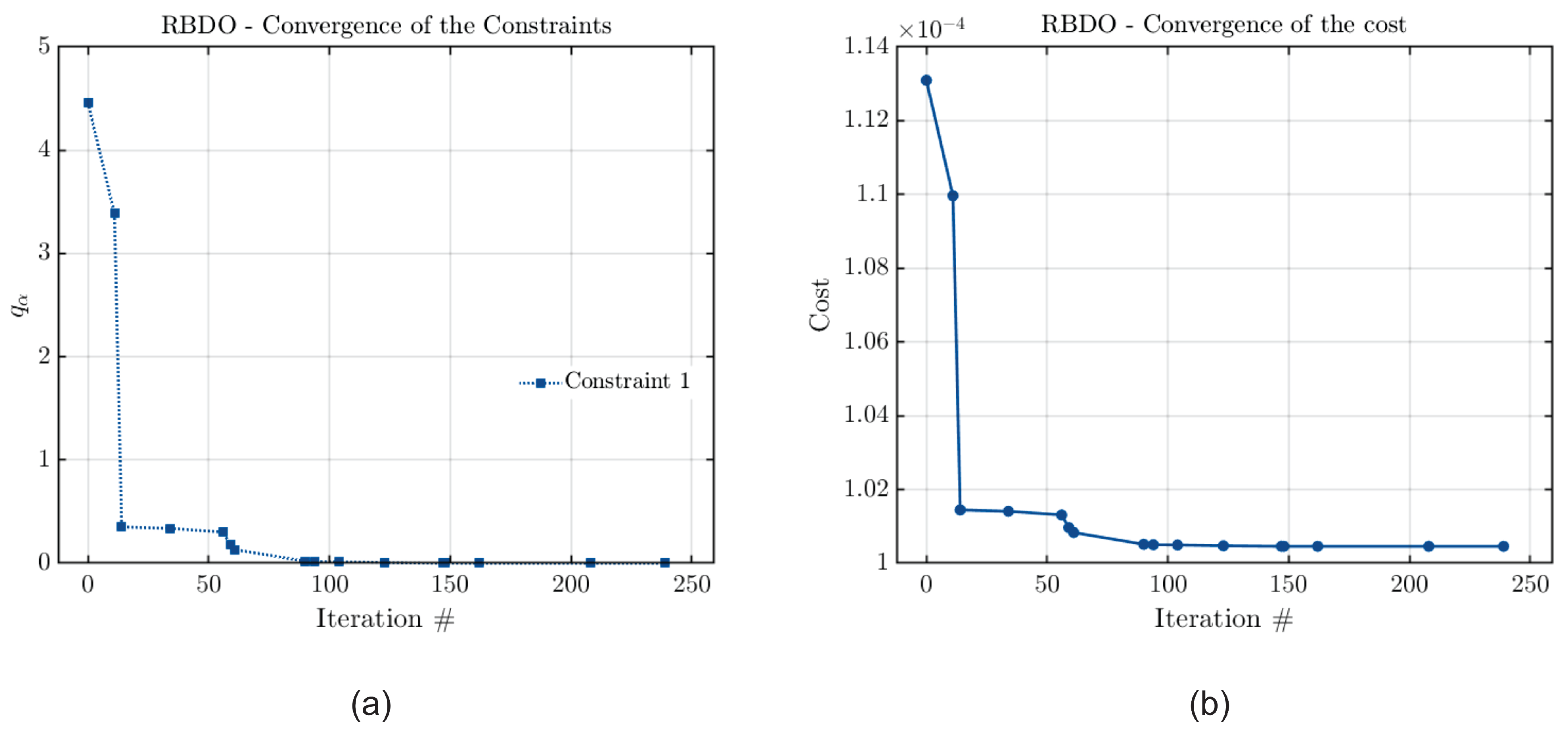
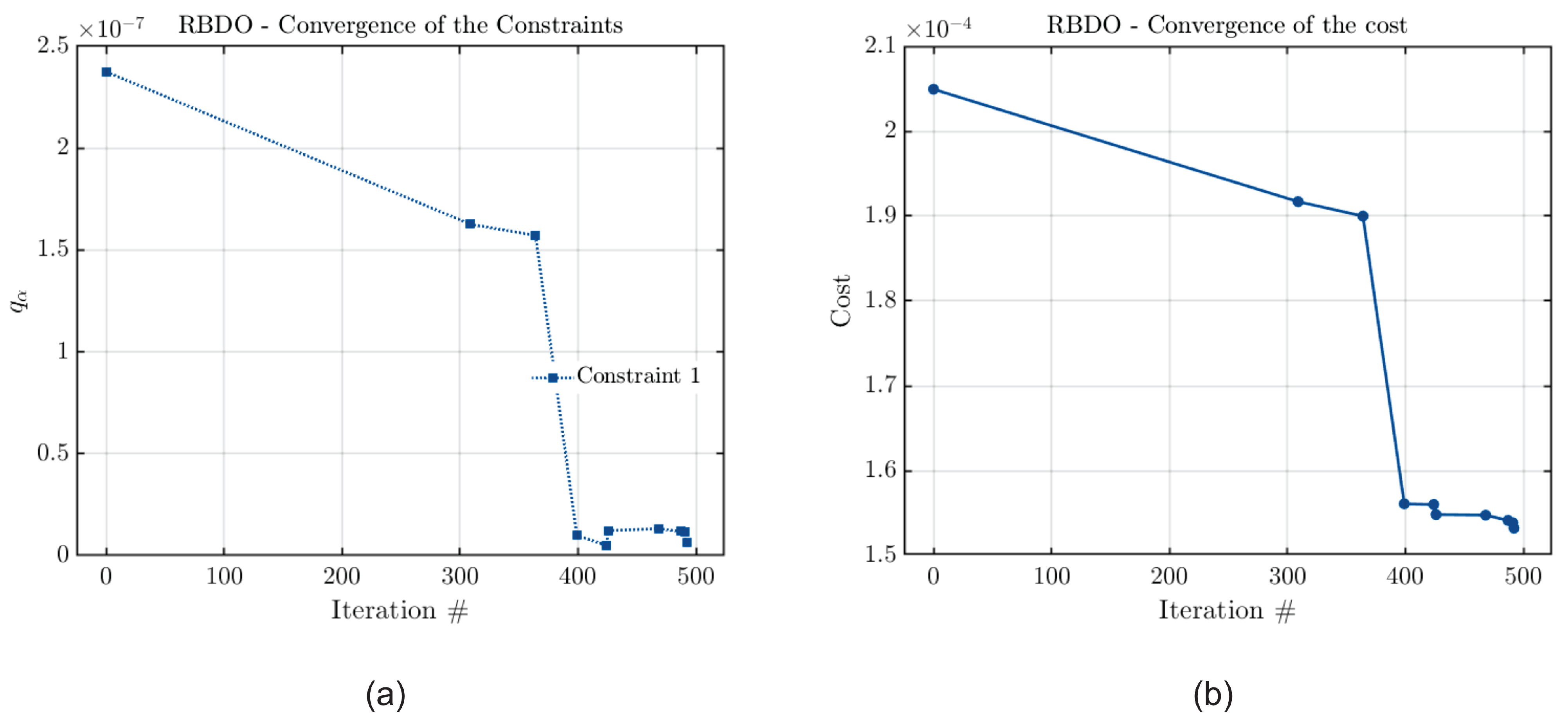
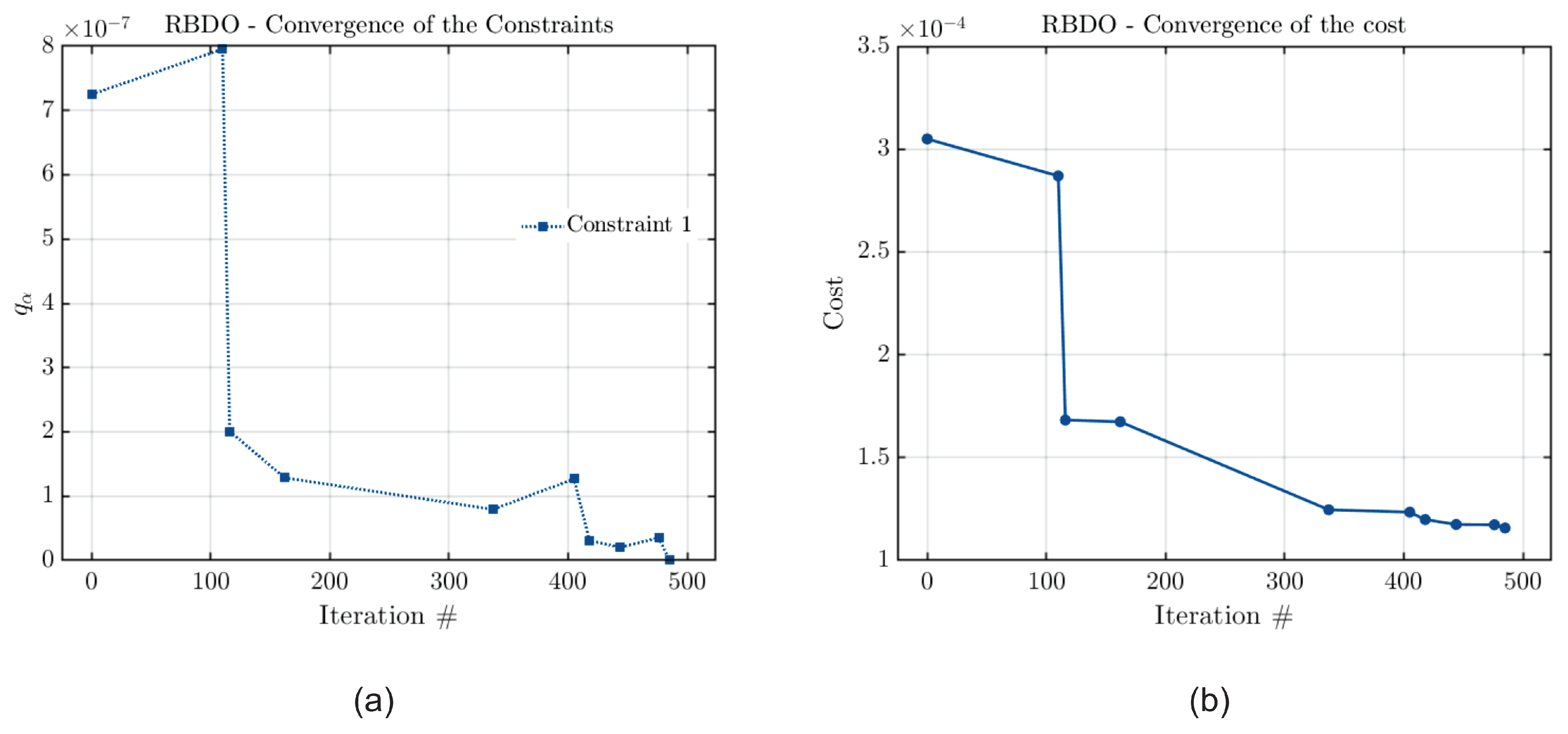
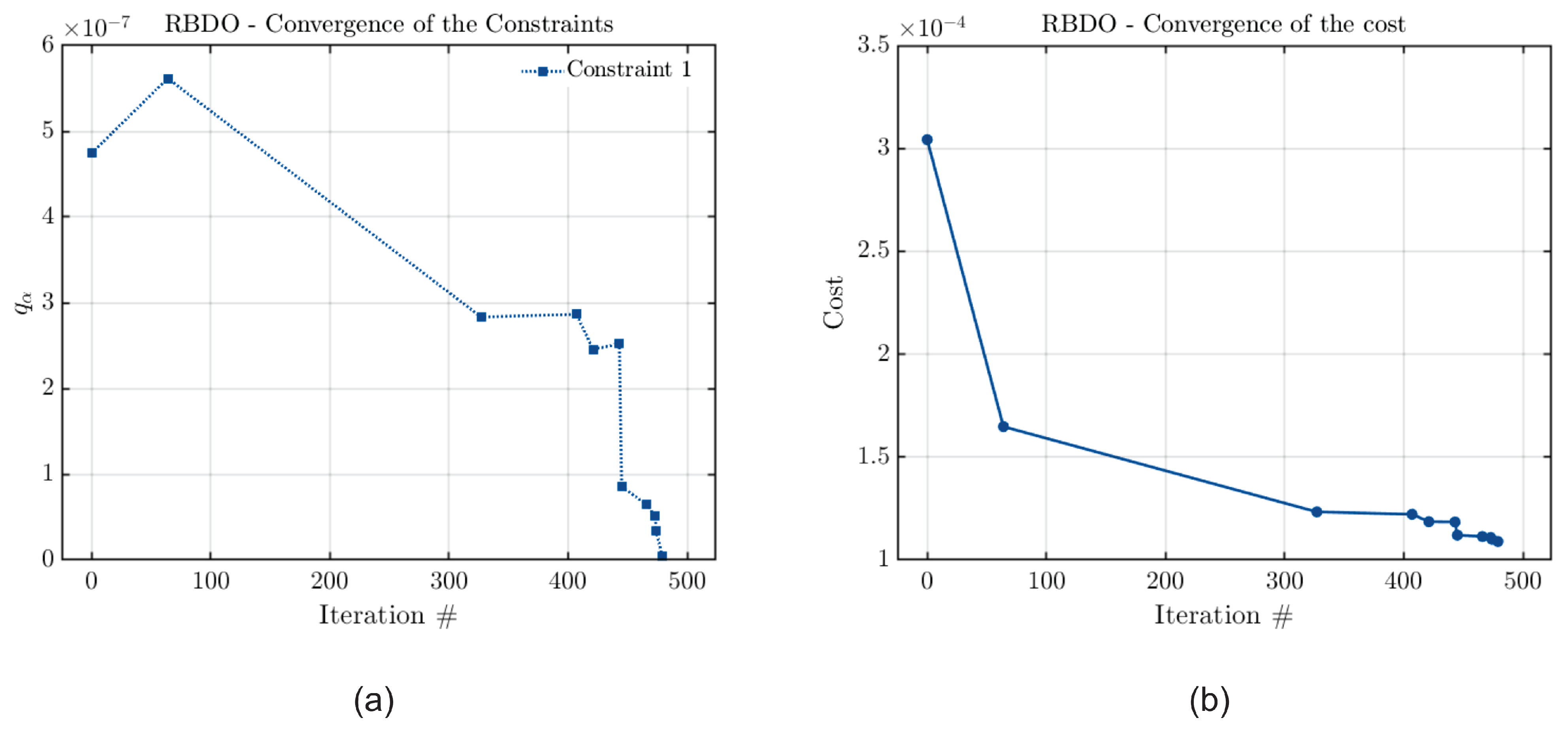
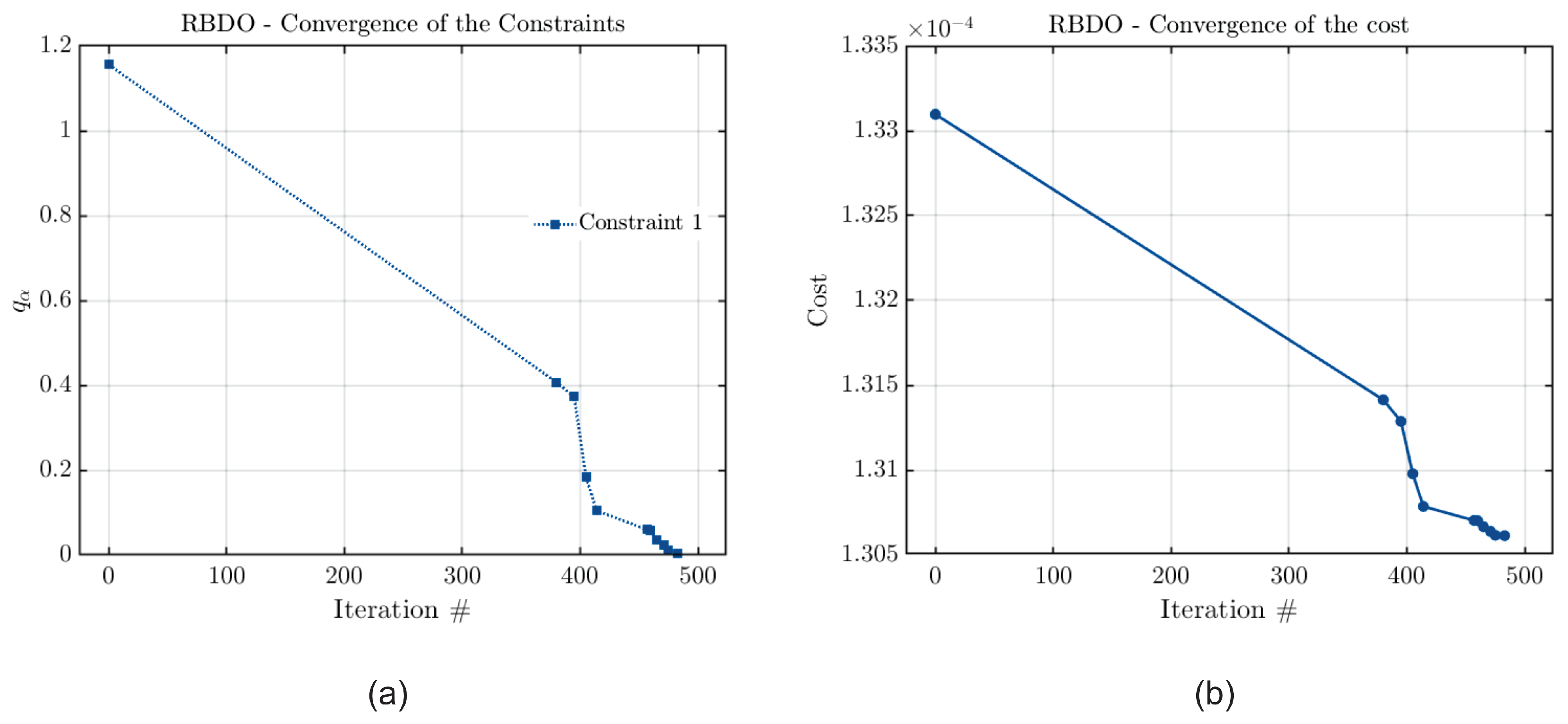
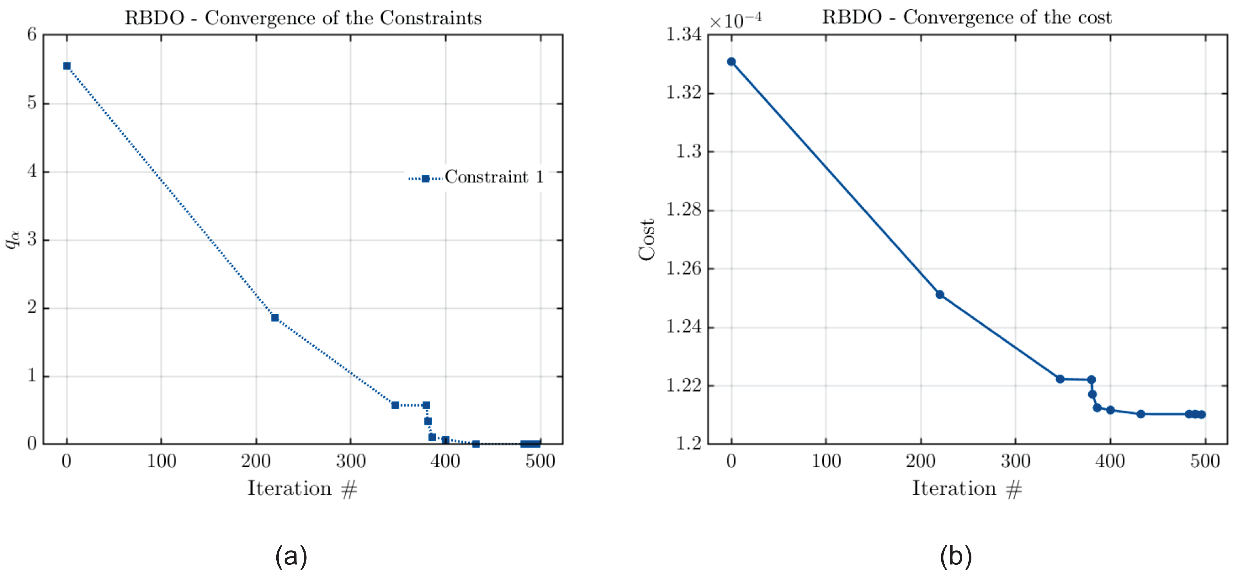
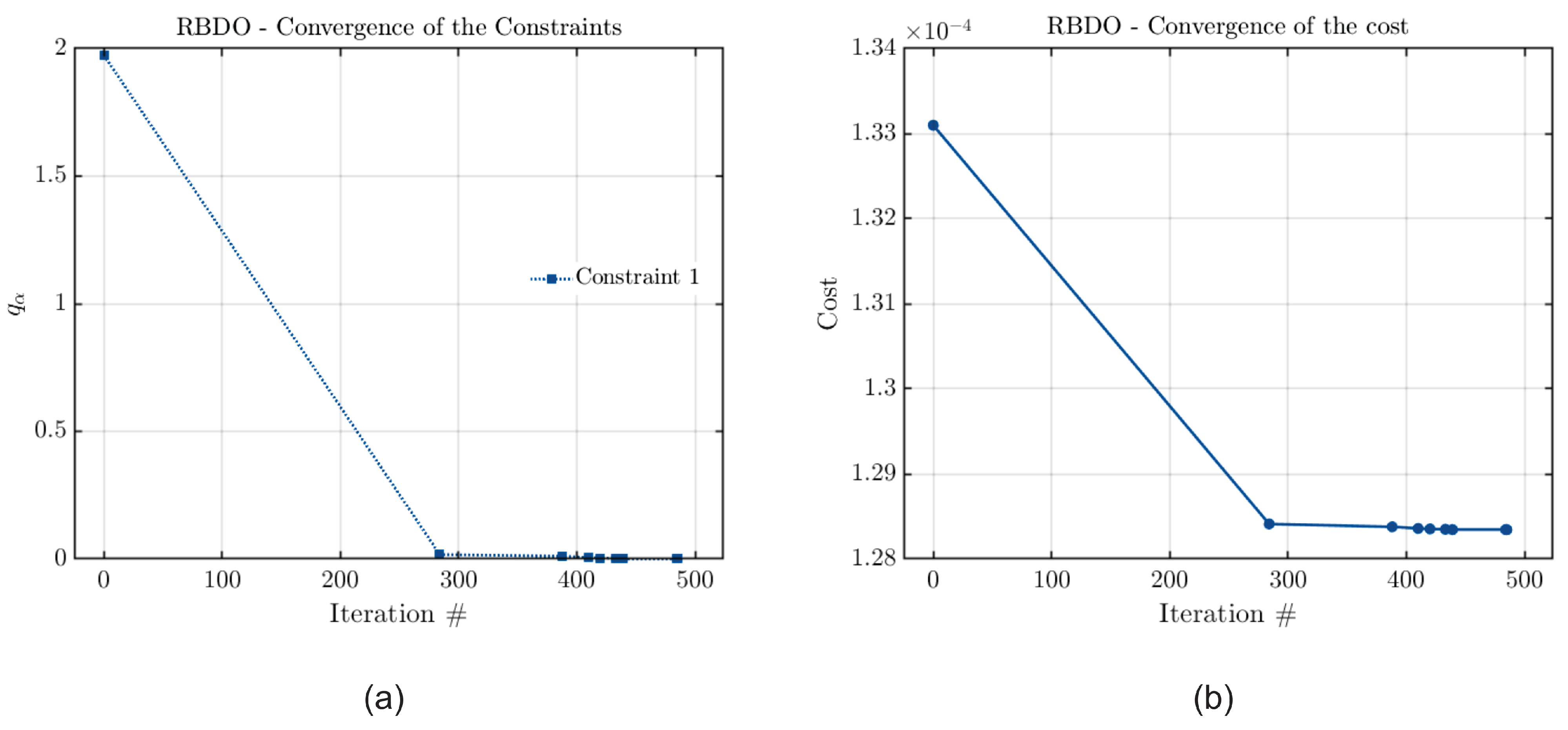
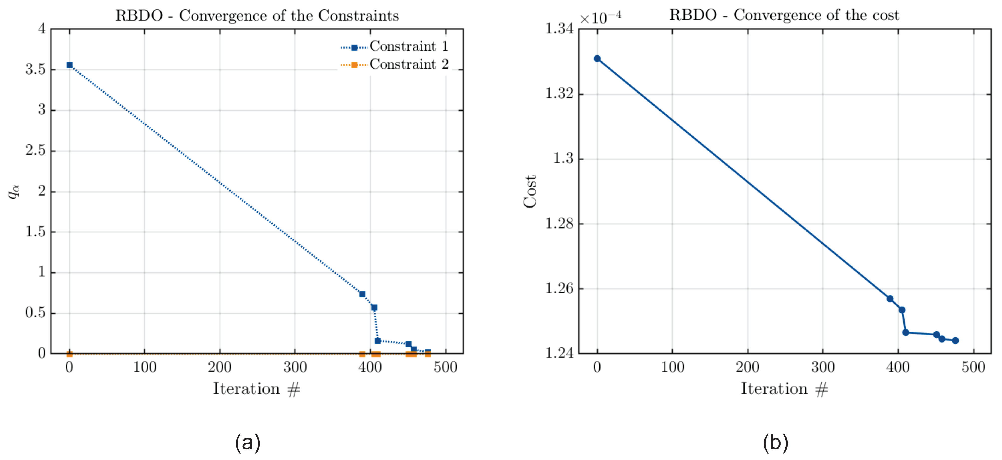
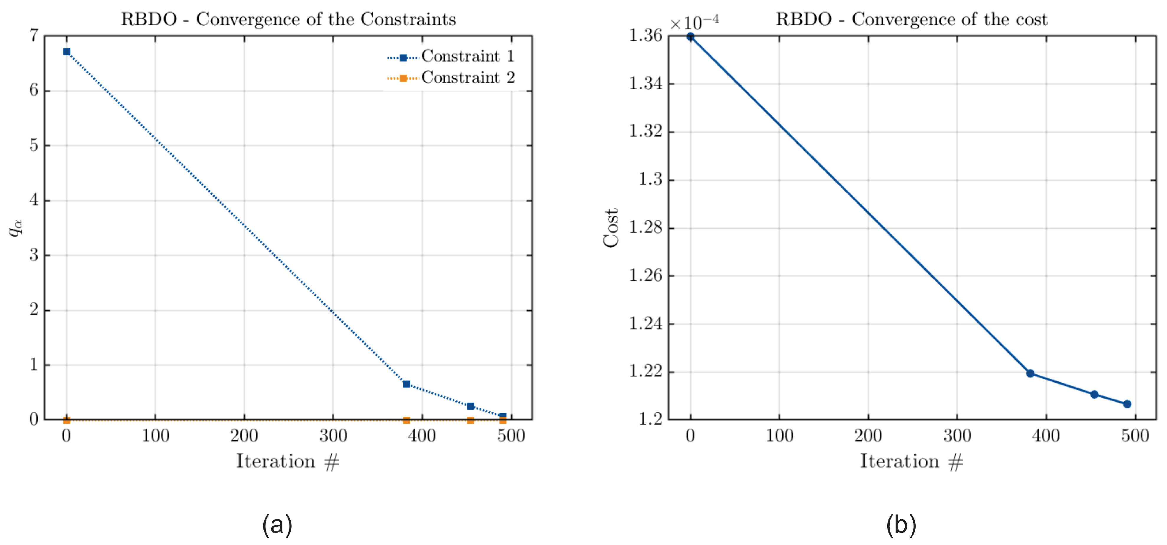
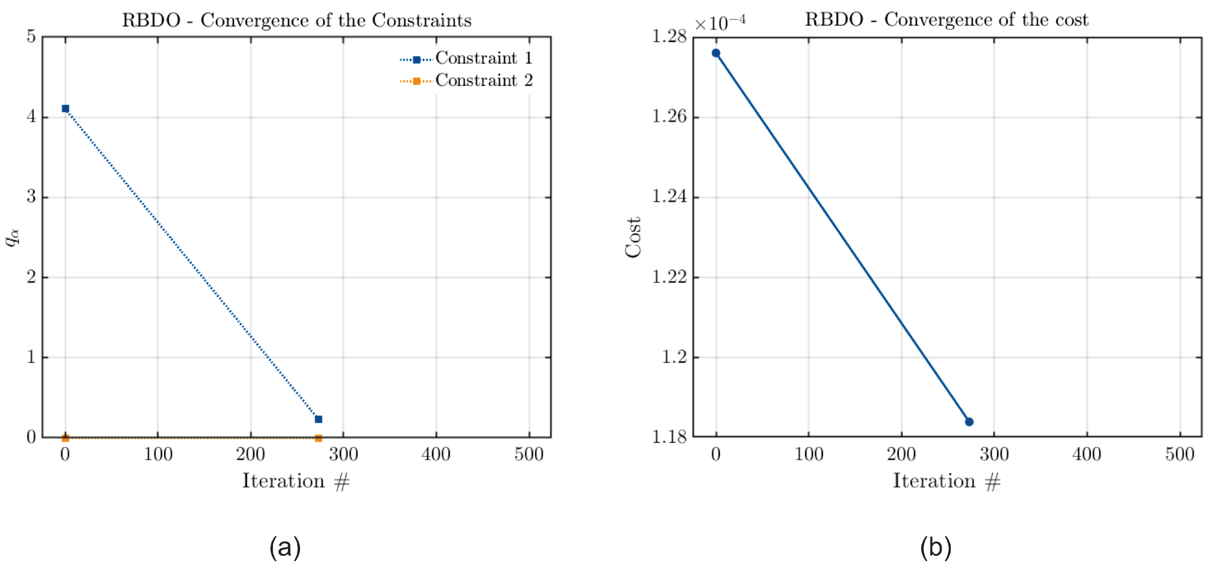
The accuracy of each model can also be verified through an analysis of the convergence curves of their cost and constraint functions. These curves are presented in Figure 2, Figure 3 and Figure 4 for the case in which the optimization constraint is the vibration amplitude limit. In all cases, the blue line indicates the evolution of the cost and constraint functions throughout each of the # iterations of the model. The blue points indicate iterations highlighted by the model, which are considered key values for the RBDO approach.

Observing Figure 2, Figure 3 and Figure 4, it is evident that the results converged for all metamodels. As these metamodels were constructed based on the QMC approach of RBDO, their convergence occurs when the convergence criteria of QMC are satisfied. Thus, the results converge when the final value calculated for the estimated quantile is zero. Observing the figures, this was the case in all instances, once again indicating that the results obtained by all methods are consistent, and any differences arise solely from potential instabilities and variations in model construction.

These results were expected, as discussed in previous sections, highlighting the capability of achieving high precision with these methods. The use of global optimization algorithms and the ability to improve the precision by increasing the number of Monte Carlo realizations contribute to the consistency of these results. Additionally, these results were obtained within an acceptable computational time due to the use of surrogate models, which significantly reduce the computational cost of each realization.

The consistency of the results obtained for the optimization of the rotor shaft diameter can be verified by plotting histograms for the rotor maximum vibration amplitude considering the shaft diameter values obtained by each metamodel. This is illustrated in Figure 5 for this configuration of the optimization problem.

Based on Figure 5, it is evident that the upper limit value for the maximum rotor vibration amplitude is consistently close to 1 $\mathsf{\mu }$m in all cases. Furthermore, when considering the frequency of values presented in the histograms that exceeded the defined vibration amplitude limit, it can be observed that, across the three metamodels, reliability of approximately $99\%$ was achieved for this system. This validates the obtained results and confirms the viability of the formulated RBDO problem in studying this rotor model configuration.

It is also noteworthy that these histograms indicate that the metamodel that obtained the smallest values for the optimal rotor shaft diameter led to the highest maximum vibration amplitudes. This observation reinforces the relationship between these two parameters, as discussed in the previous section.

Table 5. RBDO results for the rotor model considering the rotor shaft diameter optimization and the rotor’s stability threshold frequency as a constraint.

Metamodel	Diameter, mm	Evaluations	Stopping Criterion
Kriging	11.347	5,000,000	Maximum number of evaluations reached
PCE	11.858	2,160,000	Value of global step size below tolerance
PCK	11.310	2,480,000	Value of global step size below tolerance

displays the values of the optimized rotor shaft diameter for each metamodel, along with the corresponding stopping criterion that was satisfied, considering the stability threshold frequency as the optimization constraint.

Table 5 shows that the results obtained by all metamodels when considering the optimization of the rotor shaft diameter with the stability threshold frequency as a constraint are also consistent. This concordance suggests that the metamodels also converged during this optimization process, leading to global optima for all cases. As discussed for the previous optimization problem, the slight differences in the results can be justified by the instabilities of the surrogate models and differences in the construction methods for each metamodel.

From Table 5, it is also evident that, in comparison to the optimization problem that considers the limit vibration amplitude as a constraint, this case allows us to obtain smaller diameters while ensuring project reliability. Thus, it can be observed that the constraints associated with the rotor’s stability threshold are more readily satisfied by varying the rotor shaft diameter than the constraints related to its maximum vibration amplitude.

To verify each metamodel’s accuracy, the convergence curves of the cost and constraint functions when the optimization constraint is the stability threshold are presented in Figure 6, Figure 7 and Figure 8.

Figure 6, Figure 7 and Figure 8 indicate that all the metamodels’ outcomes converged, as the final value calculated for the estimated quantile is zero in all cases. Therefore, it is possible to confirm that the results obtained by all methods are consistent, with any observed differences likely arising from potential instabilities and variations in model construction. As expected, the results present good convergence and, due to the use of surrogate models, there is a low computational cost associated with the analysis.

Finally, the consistency of the results obtained can be verified by plotting histograms for the rotor’s stability threshold frequency considering the optimized shaft diameter values obtained by each metamodel. This is illustrated in Figure 9 for this configuration of the optimization problem.

Based on Figure 9, it is evident that the lower limit value for the stability threshold frequency is consistently close to 35 Hz in all cases, representing the $1\%$ failure probability of the model. Moreover, observing the frequency of values in the histograms indicating a stability threshold frequency below 35 Hz, it can be affirmed that the failure probability, constrained to a maximum of $1\%$, has been achieved for this model. This validates the obtained results and confirms the viability of the formulated RBDO problem in studying this rotor model configuration.

The results from Figure 9 also confirm the relationship between the rotor’s stability threshold and the diameter of its shaft, as discussed in the previous section. As is observable, the metamodels that obtained smaller optimal diameters exhibited the lowest values for the stability threshold frequency. This suggests that utilizing a shaft with a very small diameter may lead to stability thresholds occurring at extremely low frequencies, making rotor operation unfeasible.

Table 6. RBDO results for the rotor model considering the rotor shaft diameter optimization and both parameters as constraints.

Metamodel	Diameter, mm	Evaluations	Stopping Criterion
Kriging	12.918	2,700,000	Value of global step size below tolerance
PCE	12.940	2,860,000	Value of global step size below tolerance
PCK	12.805	2,260,000	Value of global step size below tolerance

displays the values of the optimized rotor shaft diameter for each metamodel, along with the corresponding stopping criterion that was satisfied, considering both the rotor vibration amplitude limit and stability threshold frequency as the optimization constraints.

Observing the results in Table 6, it can be seen that there is good concordance among the results obtained by all metamodels when considering the optimization of the rotor shaft diameter with both the rotor vibration amplitude limit and stability threshold frequency as constraints. This concordance indicates that, even when considering multiple constraints in the optimization problem, RBDO is still capable of providing good results for the model. Consequently, this result underscores the validity of RBDO in optimizing this rotor model while considering various parameters as constraints, given that all metamodels achieved global optima. Therefore, it can be inferred that this rotor model, and potentially other configurations of it, are suitable for the reliability-based optimization of the rotor shaft diameter.

Additionally, it can be observed that the optimal diameters obtained in this case are much closer to those obtained when considering the vibration amplitude limit of the model as a constraint than when considering the stability threshold frequency. This result aligns with the earlier discussion, since the constraint related to the vibration limit is more challenging to satisfy than the constraint related to the stability threshold frequency. Thus, to keep the maximum rotor vibration amplitude below the defined limit, the diameter needs to be larger than the diameter required to fully satisfy the stability threshold constraints. Therefore, it is evident that satisfying both constraints simultaneously is unattainable, and the stability threshold cannot be minimized to the same extent as the vibration amplitude limit.

To verify the metamodels’ accuracy, the convergence curves of the cost and constraint functions when the optimization constraints are the vibration amplitude limit and the stability threshold are presented in Figure 10, Figure 11 and Figure 12.

From Figure 10, Figure 11 and Figure 12, it is possible to see that all the metamodels have converged for the vibration limit, as the final value calculated for the estimated quantile is zero in all cases for this parameter. However, they have not converged for the stability threshold frequency. This result is understandable since, as discussed before, it is impossible to satisfy both optimization constraints. Thus, as satisfying the vibration limit constraint also ensures that the stability threshold will be above the defined minimum, this result is reasonable. However, it is impossible to further minimize the rotor shaft diameter to achieve the defined minimum value for the stability threshold frequency in this problem without exceeding the defined maximum value for its vibration amplitude. Thus, the rotor’s vibration amplitude is minimized to the greatest extent possible, while the stability threshold is minimized to remain above the defined limit but without reaching the smallest value that would be possible.

The consistency of the results obtained can be further verified by plotting histograms for the rotor’s stability threshold frequency and vibration limit amplitude considering the optimized shaft diameter values obtained by each metamodel. This is illustrated in Figure 13 and Figure 14 for this configuration of the optimization problem.

From Figure 13, it is possible to see that the upper limit of the histograms related to the maximum rotor vibration amplitude is very close to 1 $\mathsf{\mu }$m, indicating that the diameter was fully optimized to meet this constraint of the optimization design, which is only possible by obtaining a rotor stability threshold above the defined minimum frequency value. Simultaneously, from Figure 14, it is possible to see that the lower limit of the histograms related to the stability threshold frequency of the rotor is close to 42 Hz, which is above the defined limit of 35 Hz, indicating that this constraint was also met, but the rotor shaft diameter was not minimized sufficiently. As discussed earlier, it is impossible to satisfy both constraints simultaneously in this rotor configuration. Therefore, the design was optimized to minimize the rotor shaft diameter without violating any design constraints. From these results, it is possible to see that the RBDO provided valid results for this configuration of the rotor optimization project.

5.2. Rotor Shaft Diameter and Lubricating Fluid Temperature Optimization

Similarly to the previous optimization problem, in this case, the RBDO problem will consider three scenarios for its constraints: the vibration amplitude limit, the stability threshold, and both parameters. The difference is that, besides optimizing the rotor shaft diameter, the lubricating fluid temperature will also be optimized. Given that this problem involves multi-objective optimization, it is expected that the RBDO will exhibit more instability than observed in the problem discussed in the previous subsection.

Table 7. RBDO results for the rotor model considering the joint optimization and the vibration amplitude limit as a constraint.

Metamodel	Diameter, mm	Temperature, °C	Evaluations	Stopping Criterion
Kriging	12.824	24.058	5,080,000	Maximum number of generations reached
PCE	11.093	19.123	5,020,000	Maximum number of generations reached
PCK	10.838	16.682	5,040,000	Maximum number of generations reached

displays the values of the optimized shaft diameter and fluid temperature for each metamodel, along with the corresponding stopping criterion that was satisfied, considering the rotor vibration amplitude limit as the constraint.

Observing the results presented in Table 7, it is possible to see that, since there are two parameters being optimized in this problem, various configurations of the rotor shaft diameter and lubricating fluid temperature may satisfy the defined constraints for the optimization problem. If the constraints of this problem are met, all these configurations will be valid, with the most suitable one determined being based on the cost function of the problem. The cost function should define which parameter is more critical for the design (rotor shaft diameter or lubricating fluid temperature). The most important parameter has a higher weight in the weighted cost function. Since this study considers equal weights for both parameters, it is expected that both have equal importance for the design, and the optimal configuration is the one that satisfies the constraints.

An important point to highlight is that, for all metamodels, achieving a smaller rotor shaft diameter leads to a lower value for the lubricating fluid temperature. This behavior is consistent with the earlier discussion regarding the relationship of these parameters with the maximum rotor vibration amplitude. A smaller rotor shaft diameter leads to an increase in the rotor’s vibration amplitude, while a lower lubricating fluid temperature results in a reduction in the rotor’s vibration amplitude. Therefore, by reducing both parameters, there is a balance in the value of the maximum rotor vibration amplitude to satisfy this constraint in the optimization problem.

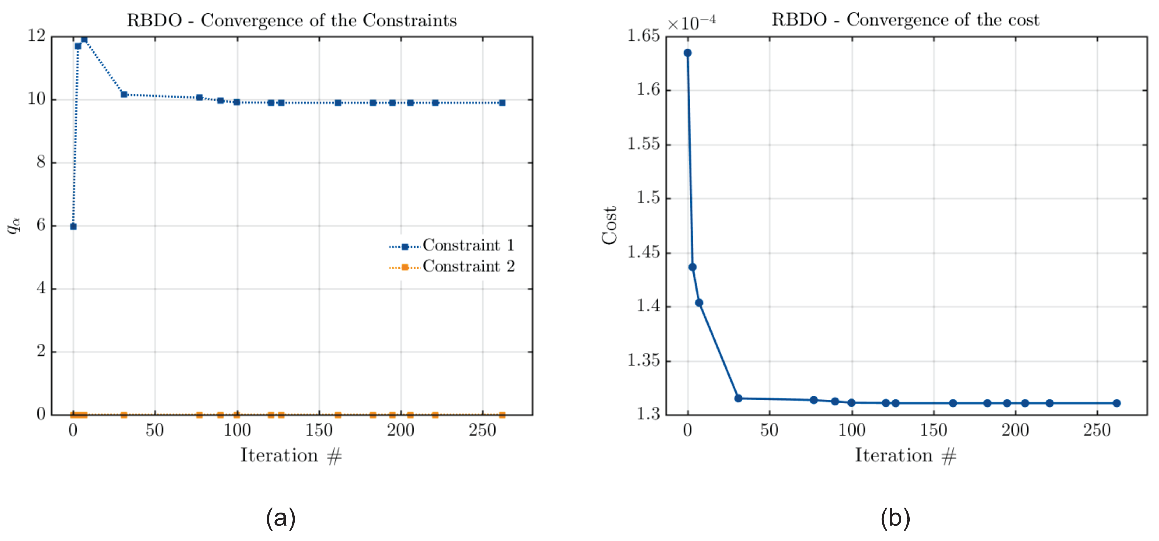
The accuracy of each metamodel can be verified through an analysis of the convergence curves of their cost and constraint functions. These curves are presented in Figure 15, Figure 16 and Figure 17 for the case in which the optimization constraint is the vibration amplitude limit.

Observing Figure 15, Figure 16 and Figure 17, it is evident that the results from PCE and PCK have fully converged, while Kriging has come very close to convergence, as the final values obtained for the estimated quantile are zero for the first two metamodels and nearly zero for the third. These results indicate consistency in the obtained outcomes, with differences in the results among the three metamodels associated with disparities in their constructions. Additionally, since the optimization involves two parameters, there will be more than one optimal configuration for the problem. Furthermore, it is noticeable that Kriging did not fully converge, explaining why it was the metamodel that obtained optimal values for the parameters that presented a greater difference from the values obtained by the other methods.

The consistency of the results for the optimization of the rotor shaft diameter can be verified by plotting histograms for the rotor maximum vibration amplitude considering the shaft diameter values obtained by each metamodel. This is illustrated in Figure 18 for this configuration of the optimization problem.

Based on Figure 18, it is evident that the upper limit value for the maximum rotor vibration amplitude is consistently close to 1 $\mathsf{\mu }$m in all cases. The results for Kriging and PCE exceed this value, while the results for PCK are below this limit. Furthermore, when considering the frequency of values presented in the histograms that surpassed the defined vibration amplitude limit, it can be observed that, across the three metamodels, reliability of approximately $99\%$ was generally achieved for this system. This validates the obtained results and confirms the viability of the formulated RBDO problem in studying this rotor model configuration, even considering multi-objective optimization.

Table 8. RBDO results for the rotor model considering the joint optimization and the rotor’s stability threshold frequency as a constraint.

Metamodel	Diameter, mm	Temperature, °C	Evaluations	Stopping Criterion
Kriging	11.885	19.680	5,000,000	Maximum number of generations
PCE	11.341	20.011	5,000,000	Maximum number of generations
PCK	11.728	20.323	5,000,000	Maximum number of generations reached

displays the values of the optimized shaft diameter and fluid temperature for each metamodel, along with the corresponding stopping criterion that was satisfied, considering the stability threshold frequency as the optimization constraint.

Observing the results in Table 8, it is possible to see that the results obtained by all metamodels are consistent when considering the optimization of the rotor shaft diameter and lubricating fluid temperature with the stability threshold frequency as a constraint. These results indicate that, unlike the case wherein the rotor vibration limit was considered as a constraint in the optimization problem, using the rotor’s stability threshold as a constraint does not allow as many different configurations that satisfy the optimization problem to be fulfilled.

These results were expected, since, as discussed earlier in this work, a reduction in the rotor diameter leads to a decrease in the stability threshold frequency. Similarly, a reduction in the lubricating fluid temperature results in a decrease in the stability threshold frequency. Therefore, as minimizing both parameters will reduce the rotor’s stability threshold, it is expected that there will be fewer parameter configurations that allow us to maintain the system’s reliability. Thus, it can be inferred that, in considering this optimization problem, obtaining an optimal rotor configuration that satisfies the rotor vibration limit constraints is achieved more straightforwardly than obtaining an optimal configuration that satisfies constraints associated with the stability threshold.

The accuracy of each metamodel can be verified through an analysis of the convergence curves of their cost and constraint functions. These curves are presented in Figure 19, Figure 20 and Figure 21 for the case in which the model constraint is the stability threshold.

Figure 19, Figure 20 and Figure 21 indicate that all the metamodels have converged, as the final value calculated for the estimated quantile is zero in all cases. Therefore, it is possible to confirm that the results obtained by all methods are consistent considering this configuration of the optimization problem. As there was not a significant difference between the optimal configurations of this model, and all metamodels converged, it is possible to affirm that the slight discrepancies in the results arise from potential instabilities and variations in metamodel construction.

The consistency of the results obtained can be verified by plotting histograms for the rotor’s stability threshold frequency considering the optimized shaft diameter values obtained by each metamodel. This is illustrated in Figure 22 for this configuration of the optimization problem.

Based on Figure 22, it is evident that the lower limit value for the stability threshold frequency is consistently close to 35 Hz in all cases. The results for PCE and PCK are very close to this value, while the results for Kriging are slightly above this limit, indicating that the stability threshold frequency in this case is slightly above the allowed minimum value. Furthermore, when considering the frequency of values presented in the histograms that surpassed the defined stability threshold frequency, it can be observed that, across the three metamodels, reliability of approximately $99\%$ was generally achieved for this system. This validates the obtained results and confirms the viability of the formulated RBDO problem in studying this rotor model configuration.

Table 9. RBDO results for the rotor model considering the joint optimization and both parameters as constraints.

Metamodel	Diameter, mm	Temperature, °C	Evaluations	Stopping Criterion
Kriging	11.532	19.966	5,000,000	Maximum number of generations reached
PCE	11.503	16.733	5,060,000	Maximum number of generations reached
PCK	11.391	16.494	5,840,000	Maximum number of generations reached

displays the values of the optimized shaft diameter and fluid temperature for each metamodel, along with the corresponding stopping criterion that was satisfied, considering both the rotor vibration amplitude limit and stability threshold frequency as the optimization constraints.

Observing Table 9, it is possible to see that the results obtained by all metamodels are similar when optimizing the rotor shaft diameter and lubricating fluid temperature, considering the rotor vibration amplitude limit and stability threshold frequency as constraints. These results indicate that, as occurred in the case in which the rotor’s stability threshold was considered as a constraint, the case in which both parameters are considered as optimization constraints does not allow as many different configurations to satisfy the optimization problem. These results are consistent, as it is expected that, to meet the strictest constraint, the model approaches more closely the configuration in which this constraint is individually satisfied.

This behavior is more evident when comparing the optimal results with both constraints and the results considering the stability threshold as the only constraint. The stability threshold is the most stringent constraint of the optimization problem. Therefore, it is anticipated that these optimal configurations obtained for the rotor will allow the stability threshold to be reduced to the defined minimum, but the maximum vibration amplitude of the rotor will not reach the allowed maximum value, as the model cannot satisfy both constraints simultaneously.

To verify the metamodels’ accuracy, the convergence curves of the cost and constraint functions when the model constraints are the vibration amplitude limit and the stability threshold are presented in Figure 23, Figure 24 and Figure 25.

From Figure 23, Figure 24 and Figure 25, it is possible to see that the constraint related to the rotor’s stability threshold has been satisfied in virtually all cases, with PCK almost reaching a final value of zero for the estimated quantile, and the other metamodels achieving these zero values. Thus, it justifies the attainment of an optimal configuration for the rotor close to the one in which only this parameter was considered as a constraint, leading to the expectation that the rotor’s stability threshold in this case is very close to the defined constraint value. At the same time, it can be observed that the values of the estimated quantile related to the vibration limit constraint are very close to zero. However, it is important to emphasize that the order of magnitude of this constraint is much smaller than that of the stability threshold. Since the values obtained for the optimal parameters are further from those obtained when only the vibration limit was considered as a constraint, it is expected that the maximum vibration value obtained in this configuration does not completely satisfy the defined limit.

The consistency of the results obtained can be further verified by plotting histograms for the rotor’s stability threshold frequency and vibration limit amplitude considering the optimized shaft diameter values obtained by each metamodel. This is illustrated in Figure 26 and Figure 27 for this configuration of the optimization problem.

From Figure 27, it is possible to see that the lower limit of the histograms related to the rotor’s stability threshold frequency is close to 35 Hz, indicating that the rotor shaft diameter and lubricating fluid temperature were fully optimized to meet this constraint of the optimization design. From Figure 26, it is also possible to see that the upper limit of the histograms related to the maximum rotor vibration amplitude is below the limit of 1 $\mathsf{\mu }$m, indicating that the parameters were not fully optimized to satisfy this constraint. As discussed earlier, it is impossible to satisfy both constraints of this optimization problem simultaneously in this rotor configuration. Therefore, to achieve the designed rotor’s stability threshold frequency, which is the strictest constraint of this optimization problem, the maximum vibration amplitude of the rotor must stay below the designed limit. Consequently, the parameters of the rotor design were optimized without violating any design constraints by fully satisfying the stability threshold constraint and meeting the vibration amplitude constraint without reaching the optimal configuration for it.

6. Conclusions

This study considered the RBDO of a rotating system. Two optimization problems were addressed: the first focused on optimizing the rotor shaft diameter, while the second aimed to optimize both the rotor shaft diameter and the operating temperature of the bearings’ lubricating fluid. In both optimization problems, the rotor’s vibration amplitude limit, its stability threshold frequency, and both parameters were considered as constraints. To solve the RBDO problem, surrogate models were utilized. The methods employed to construct the metamodels were Kriging, PCE, and PCK.

Analyzing the optimization of the rotor shaft diameter, it was possible to validate the RBDO for this model. As there was only one parameter being optimized, it was possible to obtain similar results for all methods. Additionally, since surrogate models may exhibit some instabilities during their operation, slight variations in results between different models are expected. In this study, it was observed that the constraint related to the rotor’s vibration amplitude was stricter than the constraint related to the stability threshold. Consequently, the second constraint allowed smaller diameters compared to the first one. Therefore, when considering both constraints, the maximum vibration amplitude had greater significance in determining the optimal values for the rotor shaft diameter.

Considering the optimization of the rotor shaft diameter and lubricating fluid temperature, as there were two parameters being optimized, it was expected to obtain diverse optimal configurations for the rotor. The specific optimal configurations would depend on how the model’s cost function was defined, determining the relative importance of each parameter to the model. In this study, both parameters were assigned equal weight in the cost function. It was observed that, for this problem, the constraint related to the rotor’s stability threshold was stricter than the constraint related to the vibration amplitude. Therefore, when considering both constraints, the stability threshold had greater significance than the maximum vibration amplitude in determining the optimal values for the rotor shaft diameter and lubricating fluid temperature.

Previous studies [29] have explored the application of RBDO to an idealized rotor model, achieving favorable results. However, they emphasize the need to validate this method for a more accurate rotor model. The result of this study showed that the RBDO presents coherent results when optimizing even a more complex rotor model. It was evident that the method was compatible with different constraints and parameters to be optimized, demonstrating significant applicability to rotor design. Furthermore, it was observed that, during the optimization of the model, the strictest constraint always had a greater influence in terms of obtaining optimal results, e.g., the cost function parameter with greater weight would always be prioritized. Thus, it can be observed that the determination of the design parameters to be optimized and the optimization constraints for the problem is crucial in rotor design when considering reliability-based design optimization.

References

1. Zhan, Z.; Zhang, X.; Jian, Z.; Zhang, H. Error modelling and motion reliability analysis of a planar parallel manipulator with multiple uncertainties. Mech. Mach. Theory 2018, 124, 55–72. [Google Scholar] [CrossRef]
2. Wang, W.; Gao, H.; Zhou, C.; Zhang, Z. Reliability analysis of motion mechanism under three types of hybrid uncertainties. Mech. Mach. Theory 2018, 121, 769–784. [Google Scholar] [CrossRef]
3. Wang, L.; Xiong, C.; Wang, X.; Xu, M.; Li, Y. A dimension-wise method and its improvement for multidisciplinary interval uncertainty analysis. Appl. Math. Model. 2018, 59, 680–695. [Google Scholar] [CrossRef]
4. Wang, L.; Cai, Y.; Liu, D. Multiscale reliability-based topology optimization methodology for truss-like microstructures with unknown-but-bounded uncertainties. Comput. Methods Appl. Mech. Eng. 2018, 339, 358–388. [Google Scholar] [CrossRef]
5. Wang, L.; Xiong, C.; Hu, J.; Wang, X.; Qiu, Z. Sequential multidisciplinary design optimization and reliability analysis under interval uncertainty. Aerosp. Sci. Technol. 2018, 80, 508–519. [Google Scholar] [CrossRef]
6. Cavalini, A.A.; Lara-Molina, F.A.; de Paula Sales, T.; Koroishi, E.H.; Steffen, V. Uncertainty analysis of a flexible rotor supported by fluid film bearings. Lat. Am. J. Solids Struct. 2015, 12, 1487–1504. [Google Scholar] [CrossRef]
7. Sinou, J.J.; Didier, J.; Faverjon, B. Stochastic non-linear response of a flexible rotor with local non-linearities. Int. J. Non-Linear Mech. 2015, 74, 92–99. [Google Scholar] [CrossRef]
8. Tudose, L.; Rusu, F.; Tudose, C. Optimal design under uncertainty of bearing arrangements. Mech. Mach. Theory 2016, 98, 164–179. [Google Scholar] [CrossRef]
9. Tyminski, N.C.; Tuckmantel, F.W.S.; Cavalca, K.L.; de Castro, H.F. Bayesian inference applied to journal bearing parameter identification. J. Braz. Soc. Mech. Sci. Eng. 2017, 39, 2983–3004. [Google Scholar] [CrossRef]
10. Visnadi, L.; Castro, H. Uncertainty analysis on stability of a flexible rotor with lubricated bearings. In Proceedings of the ICVRAM-ISUMA Uncertainties Congress, Florianópolis, SC, Brazil, 8–11 April 2018. [Google Scholar]
11. de Castro, H.F.; dos Santos, J.M.C.; Sampaio, R. Uncertainty analysis of rotating systems. In Proceedings of the XVII International Symposium on Dynamic Problems of Mechanics, Sao Sebastiao, SP, Brazil, 5–10 March 2017. [Google Scholar]
12. Dourado, A.; AA Cavalini, J.; V Steffen, J. Uncertainty quantification techniques applied to rotating systems: A comparative study. J. Vib. Control 2018, 24, 3010–3025. [Google Scholar] [CrossRef]
13. Garoli, G.Y.; de Castro, H.F. Generalized polynomial chaos expansion applied to uncertainties quantification in rotating machinery fault analysis. J. Braz. Soc. Mech. Sci. Eng. 2020, 42, 610. [Google Scholar] [CrossRef]
14. Jia, Z.; Yang, Y.; Zheng, Q.; Deng, W. Dynamic analysis of Jeffcott rotor under uncertainty based on Chebyshev convex method. Mech. Syst. Signal Process. 2022, 167, 108603. [Google Scholar] [CrossRef]
15. Aoues, Y.; Chateauneuf, A. Benchmark study of numerical methods for reliability-based design optimization. Struct. Multidiscip. Optim. 2010, 41, 277–294. [Google Scholar] [CrossRef]
16. Thoft-Christensen, P.; Murotsu, Y. Application of Structural Systems Reliability Theory; Springer: Berlin, Germany, 2011. [Google Scholar]
17. Fu, C.; Sinou, J.J.; Zhu, W.; Lu, K.; Yang, Y. A state-of-the-art review on uncertainty analysis of rotor systems. Mech. Syst. Signal Process. 2023, 183, 109619. [Google Scholar] [CrossRef]
18. Xu, B.; Zang, C.; Zhang, G. Intelligent Approach to Robust Design Optimization of a Rotor System due to Its Support Stiffness Uncertainty. Shock Vib. 2020, 2020, 2564679. [Google Scholar] [CrossRef]
19. Ritto, T.G.; Lopez, R.H.; Sampaio, R.; Souza de Cursi, J.E. Robust optimization of a flexible rotor-bearing system using the Campbell diagram. Eng. Optim. 2011, 43, 77–96. [Google Scholar] [CrossRef]
20. Lopez, R.H.; Ritto, T.G.; Sampaio, R.; de Cursi, J.S. A new algorithm for the robust optimization of rotor-bearing systems. Eng. Optim. 2014, 46, 1123–1138. [Google Scholar] [CrossRef]
21. Stocki, R.; Szolc, T.; Tauzowski, P.; Knabel, J. Robust design optimization of the vibrating rotor-shaft system subjected to selected dynamic constraints. Mech. Syst. Signal Process. 2012, 29, 34–44. [Google Scholar] [CrossRef]
22. Lopez, R.; Beck, A. Reliability-Based Design Optimization Strategies Based on FORM: A Review. J. Braz. Soc. Mech. Sci. Eng. 2012, 34, 506–514. [Google Scholar] [CrossRef]
23. Dizangian, B.; Ghasemi, M.R. A fast decoupled reliability-based design optimization of structures using B-spline interpolation curves. J. Braz. Soc. Mech. Sci. Eng. 2016, 38, 1817–1829. [Google Scholar] [CrossRef]
24. Huang, Z.L.; Jiang, C.; Zhou, Y.S.; Zheng, J.; Long, X.Y. Reliability-based design optimization for problems with interval distribution parameters. Struct. Multidiscip. Optim. 2017, 55, 513–528. [Google Scholar] [CrossRef]
25. Yang, M.; Zhang, D.; Han, X. New efficient and robust method for structural reliability analysis and its application in reliability-based design optimization. Comput. Methods Appl. Mech. Eng. 2020, 366, 113018. [Google Scholar] [CrossRef]
26. Wang, Z.; Zhao, D.; Guan, Y. Flexible-constrained time-variant hybrid reliability-based design optimization. Struct. Multidiscip. Optim. 2023, 66, 89. [Google Scholar] [CrossRef]
27. Feng, H.; Shangguan, W.B.; Rakheja, S. Hybrid uncertainties-based analysis and optimization methods for axial friction force of drive-shaft systems. J. Sound Vib. 2021, 511, 116320. [Google Scholar] [CrossRef]
28. Hong, S.; Lee, S.; Jun, S.; Lee, D.H.; Kang, H.; Kang, Y.S.; Yang, S.S. Reliability-based design optimization of axial compressor using uncertainty model for stall margin. J. Mech. Sci. Technol. 2011, 25, 731–740. [Google Scholar] [CrossRef]
29. de Paula, E.H. Reliability-Based Design Optimization Applied to Rotating Systems. Master’s Thesis, Graduate Program in Mechanical Engineering, State University of Campinas, Campinas, Brasil, 2023. (In Portuguese). [Google Scholar]
30. Ni, P.; Li, J.; Hao, H.; Zhou, H. Reliability based design optimization of bridges considering bridge-vehicle interaction by Kriging surrogate model. Eng. Struct. 2021, 246, 112989. [Google Scholar] [CrossRef]
31. Ling, C.; Kuo, W.; Xie, M. An Overview of Adaptive-Surrogate-Model-Assisted Methods for Reliability-Based Design Optimization. IEEE Trans. Reliab. 2023, 72, 1243–1264. [Google Scholar] [CrossRef]
32. Marelli, S.; Sudret, B. UQLab: A Framework for Uncertainty Quantification in Matlab. In Proceedings of the 2nd International Conference on Vulnerability, Risk Analysis and Management (ICVRAM2014), Liverpool, UK, 13–16 July 2014. [Google Scholar]
33. Moustapha, M.; Marelli, S.; Sudret, B. UQLab User Manual—Reliability-Based Design Optimization. Technical Report; Chair of Risk, Safety and Uncertainty Quantification; ETH Zurich: Zurich, Switzerland, 2022; Report UQLab-V2.0-115. [Google Scholar]
34. Moustapha, M.; Sudret, B.; Bourinet, J.M.; Guillaume, B. Quantile-based optimization under uncertainties using adaptive Kriging surrogate models. Struct. Multidiscip. Optim. 2016, 54, 1403–1421. [Google Scholar] [CrossRef]
35. Marelli, S.; Schöbi, R.; Sudret, B. UQLab User Manual—Structural Reliability (Rare Event Estimation). Technical Report; Chair of Risk, Safety and Uncertainty Quantification; ETH Zurich: Zurich, Switzerland, 2022; Report UQLab-V2.0-107. [Google Scholar]
36. Tsompanakis, Y.; Lagaros, N.D.; Papadrakakis, M. Structural Design Optimization Considering Uncertainties: Structures and Infrastructures Book; CRC Press: London, UK, 2008. [Google Scholar]
37. Sampaio, R.; Lima, R. Stochastic modeling and generation of samples for random variables and vectors. Notes Appl. Math. (Port.) SBMAC 2012, 70, 1–144. (In Portuguese) [Google Scholar]
38. Papaioannou, I.; Betz, W.; Zwirglmaier, K.; Straub, D. MCMC algorithms for Subset Simulation. Probabilistic Eng. Mech. 2015, 41, 89–103. [Google Scholar] [CrossRef]
39. Zhao, Y.G.; Ono, T. A general procedure for first/second-order reliabilitymethod (FORM/SORM). Struct. Saf. 1999, 21, 95–112. [Google Scholar] [CrossRef]
40. Nocedal, J.; Öztoprak, F.; Waltz, R.A. An interior point method for nonlinear programming with infeasibility detection capabilities. Optim. Methods Softw. 2014, 29, 837–854. [Google Scholar] [CrossRef]
41. Schittkowski, K. NLPQL: A FORTRAN subroutine for solving constrained nonlinear programming problems. Ann. Oper. Res. 1986, 5, 485–500. [Google Scholar] [CrossRef]
42. Srinivas, M.; Patnaik, L.M. Genetic algorithms: A survey. Computer 1994, 27, 17–26. [Google Scholar] [CrossRef]
43. Arnold, D.; Hansen, N. A (1+1)-CMA-ES for constrained optimisation. In Proceedings of the 14th International Conference on Genetic and Evolutionary Computation—GECCO’12, ACM, Philadelphia, PA, USA, 7–11 July 2012. [Google Scholar]
44. Lataniotis, C.; Wicaksono, D.; Marelli, S.; Sudret, B. UQLab User Manual—Kriging (Gaussian Process Modeling). Technical Report; Chair of Risk, Safety and Uncertainty Quantification; ETH Zurich: Zurich, Switzerland, 2022; Report UQLab-V2.0-105. [Google Scholar]
45. Santner, T.J.; Williams, B.J.; Notz, W.I. The Design and Analysis of Computer Experiments; Springer: New York, NY, USA, 2019. [Google Scholar]
46. Marelli, S.; Lüthen, N.; Sudret, B. UQLab User Manual—Polynomial Chaos Expansions. Technical Report; Chair of Risk, Safety and Uncertainty Quantification; ETH Zurich: Zurich, Switzerland, 2022; Report UQLab-V2.0-104. [Google Scholar]
47. Schöbi, R.; Marelli, S.; Sudret, B. UQLab User Manual—Polynomial Chaos Kriging. Technical Report, Chair of Risk, Safety and Uncertainty Quantification; ETH Zurich: Zurich, Switzerland, 2022; Report UQLab-V2.0-109. [Google Scholar]
48. Schöbi, R.; Sudret, B.; Wiart, J. Polynomial-Chaos-Based Kriging. Int. J. Uncertain. Quantif. 2015, 5, 171–193. [Google Scholar] [CrossRef]
49. Schöbi, R.; Sudret, B.; Marelli, S. Rare Event Estimation Using Polynomial-Chaos Kriging. ASCE-ASME J. Risk Uncertain. Eng. Syst. Part A: Civ. Eng. 2017, 3, D4016002. [Google Scholar] [CrossRef]
50. Blatman, G.; Sudret, B. Adaptive sparse polynomial chaos expansion based on least angle regression. J. Comput. Phys. 2011, 230, 2345–2367. [Google Scholar] [CrossRef]
51. Nelson, H.D.; McVaugh, J.M. The Dynamics of Rotor-Bearing Systems Using Finite Elements. J. Eng. Ind. 1976, 98, 593–600. [Google Scholar] [CrossRef]
52. Visnadi, L.B.; de Castro, H.F. Influence of bearing clearance and oil temperature uncertainties on the stability threshold of cylindrical journal bearings. Mech. Mach. Theory 2019, 134, 57–73. [Google Scholar] [CrossRef]
53. Krämer, E. Dynamics of Rotors and Foundations; Springer: Berlin/Heidelberg, Germany; New York, NY, USA, 1993. [Google Scholar]
54. Holmes, R. The Vibration of a Rigid Shaft on Short Sleeve Bearings. J. Mech. Eng. Sci. 1960, 2, 337–341. [Google Scholar] [CrossRef]
55. Roelands, C.J.A.; Winer, W.O.; Wright, W. Correlational aspects of the viscosity-temperature-pressure relationship of lubricating oils (Dr In dissertation at Technical University of Delft, 1966). J. Lubr. Tech. 1971, 93, 209–210. [Google Scholar] [CrossRef]
Figure 1. Rotor coordinate system and finite element method illustration.
Machines 12 00233 g001
Figure 2. Convergence curves of (a) the constraint and (b) the cost functions considering Kriging, with the rotor shaft diameter optimization and the vibration amplitude limit as a constraint.
Machines 12 00233 g002
Figure 3. Convergence curves of (a) the constraint and (b) the cost functions considering PCE, with the rotor shaft diameter optimization and the vibration amplitude limit as a constraint.
Machines 12 00233 g003
Figure 4. Convergence curves of (a) the constraint and (b) the cost functions considering PCK, with the rotor shaft diameter optimization and the vibration amplitude limit as a constraint.
Machines 12 00233 g004
Figure 5. Histogram of the maximum rotor vibration amplitude considering the rotor shaft diameter optimization and the vibration amplitude limit as a constraint. Results were obtained using (a) Kriging, (b) PCE, and (c) PCK.
Machines 12 00233 g005
Figure 6. Convergence curves of (a) the constraint and (b) the cost functions considering Kriging, with the rotor shaft diameter optimization and the rotor’s stability threshold frequency as a constraint.
Machines 12 00233 g006
Figure 7. Convergence curves of (a) the constraint and (b) the cost functions considering PCE, with the rotor shaft diameter optimization and the rotor’s stability threshold frequency as a constraint.
Machines 12 00233 g007
Figure 8. Convergence curves of (a) the constraint and (b) the cost functions considering PCK, with the rotor shaft diameter optimization and the rotor’s stability threshold frequency as a constraint.
Machines 12 00233 g008
Figure 9. Histogram of the stability threshold frequency considering the rotor shaft diameter optimization and the stability threshold frequency as a constraint. Results were obtained using (a) Kriging, (b) PCE, and (c) PCK.
Machines 12 00233 g009
Figure 10. Convergence curves of (a) the constraint and (b) the cost functions considering Kriging, with the rotor shaft diameter optimization and both parameters as constraints.
Machines 12 00233 g010
Figure 11. Convergence curves of (a) the constraint and (b) the cost functions considering PCE, with the rotor shaft diameter optimization and both parameters as constraints.
Machines 12 00233 g011
Figure 12. Convergence curves of (a) the constraint and (b) the cost functions considering PCK, with the rotor shaft diameter optimization and both parameters as constraints.
Machines 12 00233 g012
Figure 13. Histogram of the maximum rotor vibration amplitude considering the rotor shaft diameter optimization and both parameters as constraints. Results were obtained using (a) Kriging, (b) PCE, and (c) PCK.
Machines 12 00233 g013
Figure 14. Histogram of the stability threshold frequency considering the rotor shaft diameter optimization and both parameters as constraints. Results were obtained using (a) Kriging, (b) PCE, and (c) PCK.
Machines 12 00233 g014
Figure 15. Convergence curves of (a) the constraint and (b) the cost functions considering Kriging, with the joint optimization and the vibration amplitude limit as a constraint.
Machines 12 00233 g015
Figure 16. Convergence curves of (a) the constraint and (b) the cost functions considering PCE, with the joint optimization and the vibration amplitude limit as a constraint.
Machines 12 00233 g016
Figure 17. Convergence curves of (a) the constraint and (b) the cost functions considering PCK, with the joint optimization and the vibration amplitude limit as a constraint.
Machines 12 00233 g017
Figure 18. Histogram of the maximum rotor vibration amplitude considering the joint optimization and the vibration amplitude limit as a constraint. Results were obtained using (a) Kriging, (b) PCE, and (c) PCK.
Machines 12 00233 g018
Figure 19. Convergence curves of (a) the constraint and (b) the cost functions considering Kriging, with the joint optimization and the rotor’s stability threshold frequency as a constraint.
Machines 12 00233 g019
Figure 20. Convergence curves of (a) the constraint and (b) the cost functions considering PCE, with the joint optimization and the rotor’s stability threshold frequency as a constraint.
Machines 12 00233 g020
Figure 21. Convergence curves of (a) the constraint and (b) the cost functions considering PCK, with the joint optimization and the rotor’s stability threshold frequency as a constraint.
Machines 12 00233 g021
Figure 22. Histogram of the stability threshold frequency considering the joint optimization and the stability threshold frequency as a constraint. Results were obtained using (a) Kriging, (b) PCE, and (c) PCK.
Machines 12 00233 g022
Figure 23. Convergence curves of (a) the constraint and (b) the cost functions considering Kriging, with the joint optimization and both parameters as constraints.
Machines 12 00233 g023
Figure 24. Convergence curves of (a) the constraint and (b) the cost functions considering PCE, with the joint optimization and both parameters as constraints.
Machines 12 00233 g024
Figure 25. Convergence curves of (a) the constraint and (b) the cost functions considering PCK, with the joint optimization and both parameters as constraints.
Machines 12 00233 g025
Figure 26. Histogram of the maximum rotor vibration amplitude considering the joint optimization and both parameters as constraints. Results were obtained using (a) Kriging, (b) PCE, and (c) PCK.
Machines 12 00233 g026
Figure 27. Histogram of the stability threshold frequency considering the joint optimization and both parameters as constraints. Results were obtained using (a) Kriging, (b) PCE, and (c) PCK.
Machines 12 00233 g027