Applying the MIMO BP Neural Network and Cloud-Based Monitoring of Thermal Behavior for High-Speed Motorized Spindle Units

Abstract

Understanding the temperature–working condition relationship is crucial for optimizing machining processes to ensure dimensional accuracy, surface finish quality, and overall spindle longevity. Monitoring and controlling spindle temperature through appropriate cooling systems and operational parameters are essential for efficient and reliable machining operations. This paper presents an in-depth analysis of the thermal equilibrium and deformation characteristics of a high-speed motorized spindle unit utilized in grinding machine tools. Through a series of thermal equilibrium experiments and meticulous data acquisition, the study investigates the nuanced influence of various working conditions, including spindle speeds, coolant types, and coolant flow rates, on spindle temperatures and thermal deformations. Leveraging the power of Artificial Neural Networks (ANNs), predictive models are meticulously developed to accurately forecast spindle behavior. Subsequently, the models are seamlessly transitioned to a cloud computing infrastructure to ensure remote accessibility and scalability, facilitating real-time monitoring and forecasting of spindle performance. The validity and reliability of the predictive models are rigorously assessed through comparison with experimental data, demonstrating excellent agreement and high accuracy in forecasting spindle thermal behavior. Furthermore, the study underscores the critical role of key working condition variables as precise predictors of spindle temperature and thermal deformation, emphasizing their significance in optimizing overall spindle efficiency and performance. This comprehensive analysis offers valuable insights and practical implications for enhancing spindle operation and advancing the field of grinding machine tools.

1. Introduction

With the continuous progress of industrial technology, especially in the era of Industry 4.0, the accuracy requirements of high-speed machine tools are becoming increasingly significant.

The development of technology for high-speed machine tool manufacturing must be observed from the point of view of machine tool applications. Before any further consideration, it is essential to address whether a spindle is intended for machining with high cutting force or high speeds. In the first case, the spindle stiffness is the more important characteristic, while in the second case, the specific speed coefficient is important. Machine tools’ exploitation characteristics, such as accuracy, which defines the workpiece quality; productivity, which defines the speed of the working process; and profitability, which defines the speed of return on investment, depend on the vital assembly behavior.

The high-speed motorized spindle is one of the core components that influence the machining precision and productivity of machine tools. The factors affecting the machine tools’ accuracy can be divided into four different categories, namely, geometric, kinematic, thermal, and cutting-force-induced errors. Elevated temperatures during machining with a high-speed spindle often result in thermal expansion. Variances in temperature-induced expansion and contraction rates between the spindle and workpiece can lead to deviations from the intended dimensions. On the other hand, rising temperatures may also cause thermal gradients in the spindle, leading to uneven thermal expansion. This can induce vibrations and deflections in the spindle structure, impacting machining accuracy. Thermal errors can appear from the heat generated during the machining process, leading to deformations and deviations in the spindle. A comprehensive examination of thermal error modeling techniques investigated and utilized over the last decade was provided in [1]. The motorized spindle itself can contribute to heat generation through energy losses, such as electrical losses in the motor and mechanical losses in the bearings. The material composition of the spindle affects its coefficient of thermal expansion. As the spindle heats up during machining, temperature distribution across the spindle will not be uniform as it expands. Certain areas may experience higher temperatures than others, leading to uneven thermal expansion, which may result in dimensional changes in the spindle components. Thermal growth on the spindle components produces thermal expansion of bearing elements, causing the so-called thermal preload. The temperature can have a significant influence on the preload in high-speed spindles, particularly in precision machining applications where tight tolerances are critical. Understanding the influence of temperature on preload is crucial for maintaining the performance and accuracy of high-speed spindles. Regular maintenance and monitoring of temperature conditions during operation are essential to ensure consistent performance over time. The percentage of thermal errors in total machine tool errors is between 40 and 80% [2,3]. On the other hand, bearing deformations account for 30 to 50% of total spindle deformations [4].

Thermal behavior analysis and modeling for high-speed motorized spindles are crucial aspects of precision machining, especially in applications where tight tolerances and high accuracy are required. Analyzing and modeling thermal behavior in high-speed motorized spindles is a complex task that requires a combination of advanced techniques, such as experimental testing, numerical modeling, regression analysis, artificial neural networks (ANNs), and a combination of various modeling methods (hybrid modeling).

An automatic modeling algorithm employing the Chebyshev polynomial-based orthogonal least squares regression was proposed by Li et al. [5] to improve the modeling accuracy and the efficiency of the geometric error components. Determining the best position of the temperature sensor by covariance characteristic of the least square value was performed by Naumann et al. [6]. Multiple regressions were utilized to establish a connection between one dependent variable and one or more independent variables through statistical analysis of the experimental sample data. Chen et al. [7] used multivariate regression modeling to find the right coefficient to ensure that the residual is equal at each data point and the objective function (thermal error) value is minimized. An improved linear multiple regression model was presented in [8]. The original objective function was extended by incorporating the additional weighted terms related to robust criterion functions, typically taking values smaller than one as residuals increase. The proposed method demonstrated its effectiveness in enhancing the accuracy of machine tools. Shi et al. [9] and Zhang et al. [10] determined the thermal deformation of screw shafts using thermal expansion definition-based calculation and multiple regression analysis, which required the collection of the critical temperature variables.

Application of regression analysis to a multiple-output variable model is difficult. In contrast to employing a regression model, the thermal behavior of the spindle with multiple variables can be represented by a single neural network, using multiple neurons as outputs at the last layer.

As early as the end of the last century, various types of artificial neural networks have been proposed for the thermal error modeling of machine tools, e.g., backpropagation (BP) [11,12,13,14,15], radial basis function (RBF) [16,17,18], Elam Network (EN) [19], Grey Neural Networks (GNN) [20,21], etc.

Hao et al. [11] used a genetic algorithm (GA)-based BPANNs to improve the accuracy of the prediction of thermal deformation in the turning center. A combination of a genetic algorithm (GA) and BP modeling is proposed in [12] and Ma [22], where GA is used to optimize the initial weights and threshold values of the BP network until these values meet the accuracy requirements. Yang et al. [13] analyzed how different spindle speeds affect thermal characteristics, using a fuzzy clustering regression analysis method to optimize variables representing thermal error sensitivity. A BP neural network with multi-input and multi-output (MIMO) for the spindle axial thermal deformation and radial thermal errors was used. Guo et al. [23] optimized temperature-sensitive points by grey correlation and clustering analysis and defined the prediction model using a BP neural network with its parameters (weights and thresholds) optimized using an artificial fish swarm algorithm (FSA) and ant colony algorithm (ACA). Optimization of weights and thresholds of the BP neural network using a particle swarm algorithm (PSA) and beetle antennae search algorithm (BAS) was performed by Li et al. [14,15]. To improve the accuracy of thermal characteristics analysis of motorized spindle, an online correction model of thermal boundary conditions is proposed based on the BP neural network (BPNN), using experimental data and simulation results to construct the BPNN model to correct the thermal boundary conditions of the motorized spindle. Kosarac et al. [24] used BP neural networks with the Adam optimization algorithm to optimize the initial weights, thresholds, and number of hidden layer neurons for the prediction of the temperature of motorized spindle units under different input conditions. Thermal characteristics analysis of a motorized spindle employing an online correction model of thermal boundary conditions based on a BP neural network was proposed by Yi and Fan [25]. In this case, experimental data and simulation results were used to construct the BP model to correct the thermal boundary conditions of the motorized spindle. Based on the cosimulation of different software, a digital twin system for thermal characteristics was built to accurately forecast the temperature field and thermal deformation of a motorized spindle under varied operating conditions. The experimental results showed that the prediction accuracy of the temperature field is greater than 98%, and the prediction accuracy of thermal deformation is greater than 96%.

Prediction models of thermal errors obtained by using the multiple linear regressions (MLR) method, BP neural network method, and Radial Basis Function (RBF), were proposed in [26]. The results of those experiments indicate that such models can represent the thermal characteristics of the motorized spindle, while their degree of confidence mainly depends on the setting of thermal load and boundary conditions; also, based on the test data, the RBF neural network model exhibits the highest prediction precision and superior robustness for thermal errors in the motorized spindle. Fu et al. [18] used a chicken swarm optimization algorithm (CSO)-based RBF neural network model for thermal error modeling of machine tool spindle. Firstly, the so-called KC-RBF, an integrated approach that includes K-means clustering, correlation analysis, and RBF neural network, was proposed to select temperature-sensitive points. Secondly, the RBF neural network is introduced for thermal error modeling. At the same time, the CSO algorithm was used to optimize the initial parameters of the RBF to improve the prediction accuracy of the model. Also, Zhang [17] constructed the thermal error prediction model, using a PSA to optimize the weights and thresholds of the RBF neural network.

A thermal error prediction model based on the combination of a long short-term memory (LSTM) and convolutional neural network (CNN) was proposed by Cheng et al. [27]. The K-harmonic means (KHM) clustering algorithm and grey relational analysis method (GRA) were used to optimize the temperature measurement points. Then, an LSTM-CNN thermal error prediction model was established and compared with the conventional model in terms of prediction performance and robustness. The results reveal that the presented thermal error model is significantly better than the conventional model. To improve the spindle thermal error prediction accuracy, the least absolute shrinkage and selection operator (LASSO) was used by [28] to directly select the temperature-sensitive point subset to guarantee the prediction performance of the thermal error model constructed using support vector machines (SVM).

By uploading and streaming data to the cloud, manufacturers can harness the computational power and scalability of cloud-based analytics tools. This enables predictive analytics, anomaly detection, optimization algorithms, and other AI-driven capabilities to enhance efficiency, quality, and agility in manufacturing operations [29]. Enhanced dynamic scheduling methodologies coupled with refined optimization algorithms in cloud manufacturing contexts were proposed in [30]. Khdoudi et al. [31] presented a comprehensive framework for implementing a full-duplex digital twin system tailored for autonomous process control. Milosevic et al. [32] presented a developed cloud-based system for monitoring the condition of cutting tool wear by measuring vibration. This system applies a machine learning method that is integrated within the MS Azure cloud system.

In the above-mentioned papers, temperature variables tested by multiple sensors are taken as inputs, while thermal errors of machine tools are provided as outputs of various NN models. After the network learning and training procedures had been completed, the thermal errors of machine tools in multiple directions were accurately fitted and predicted.

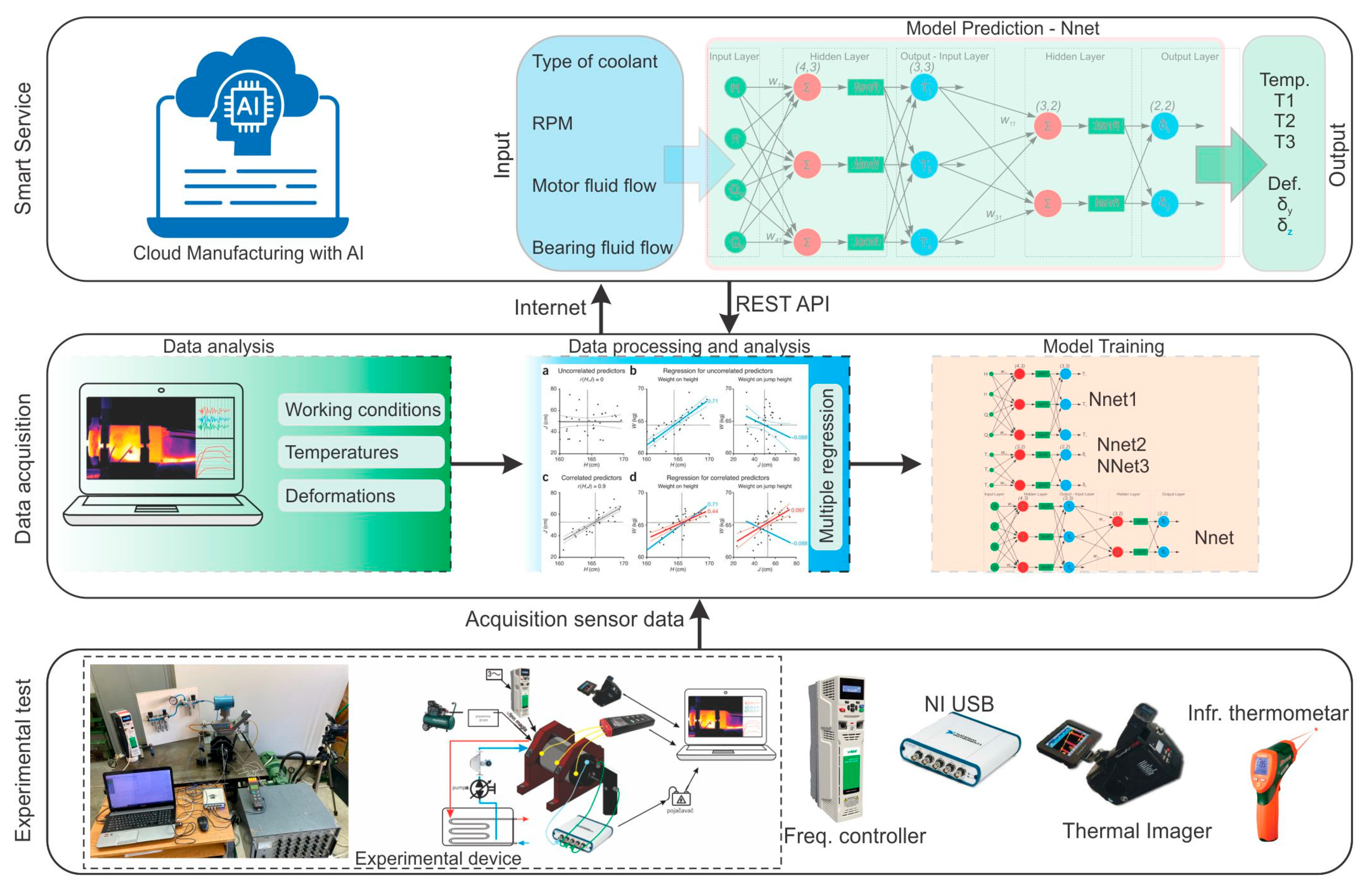
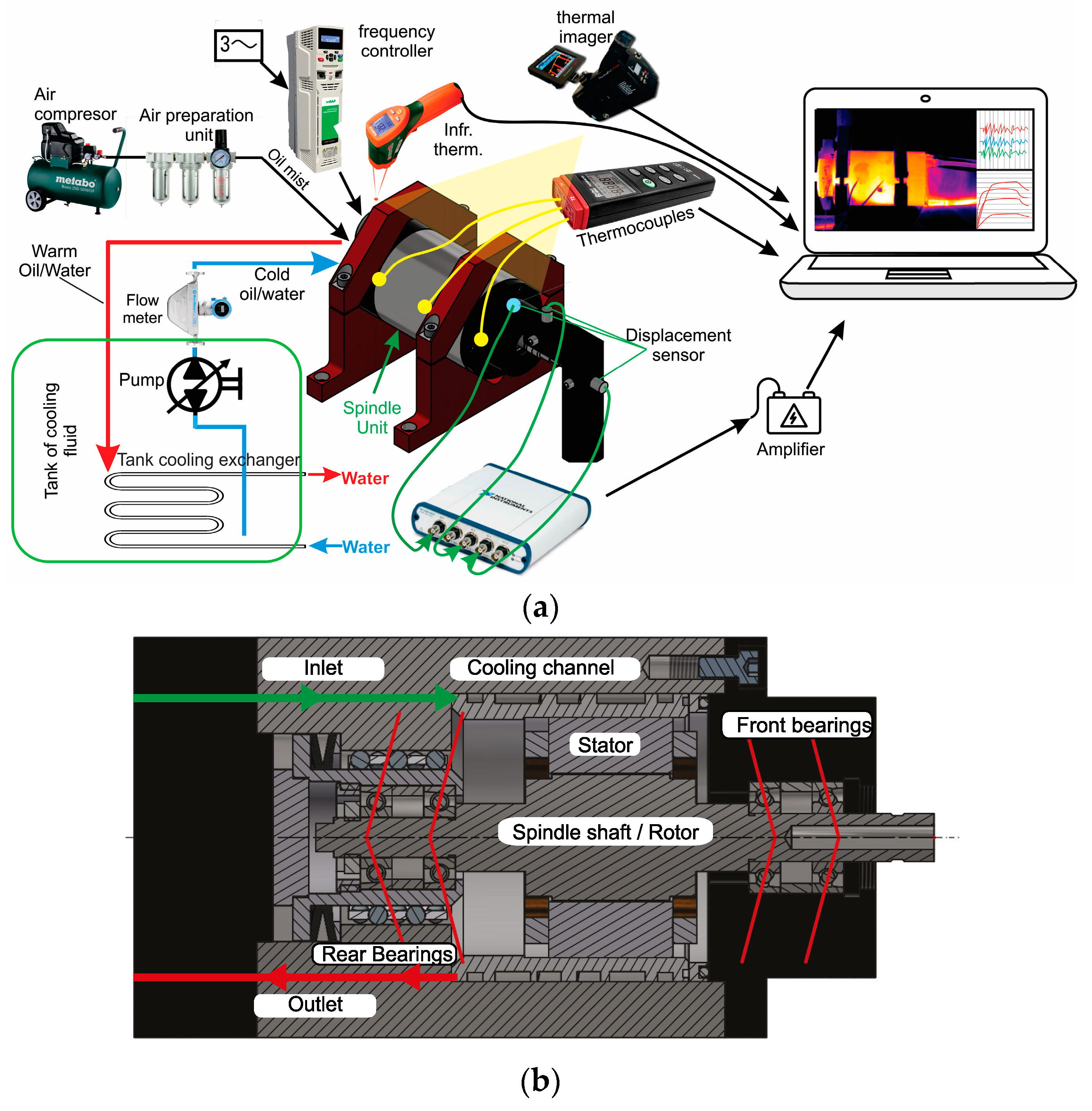
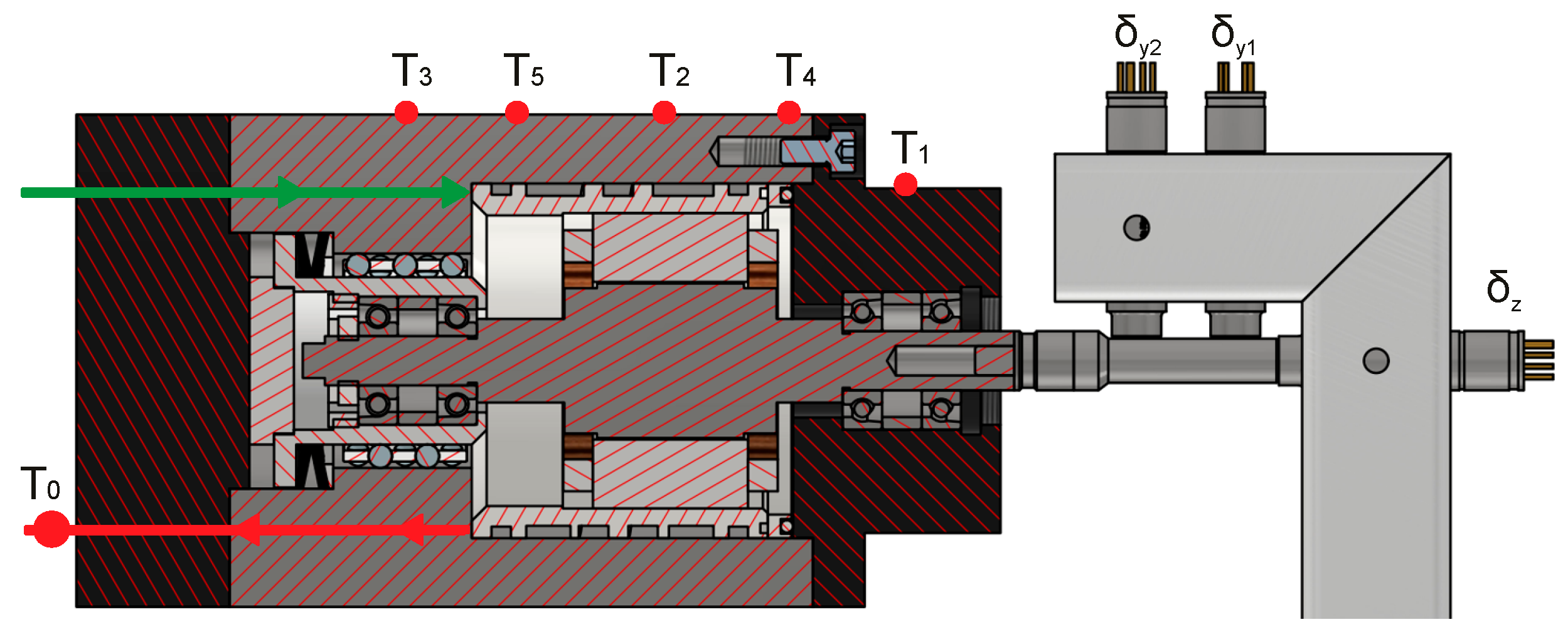
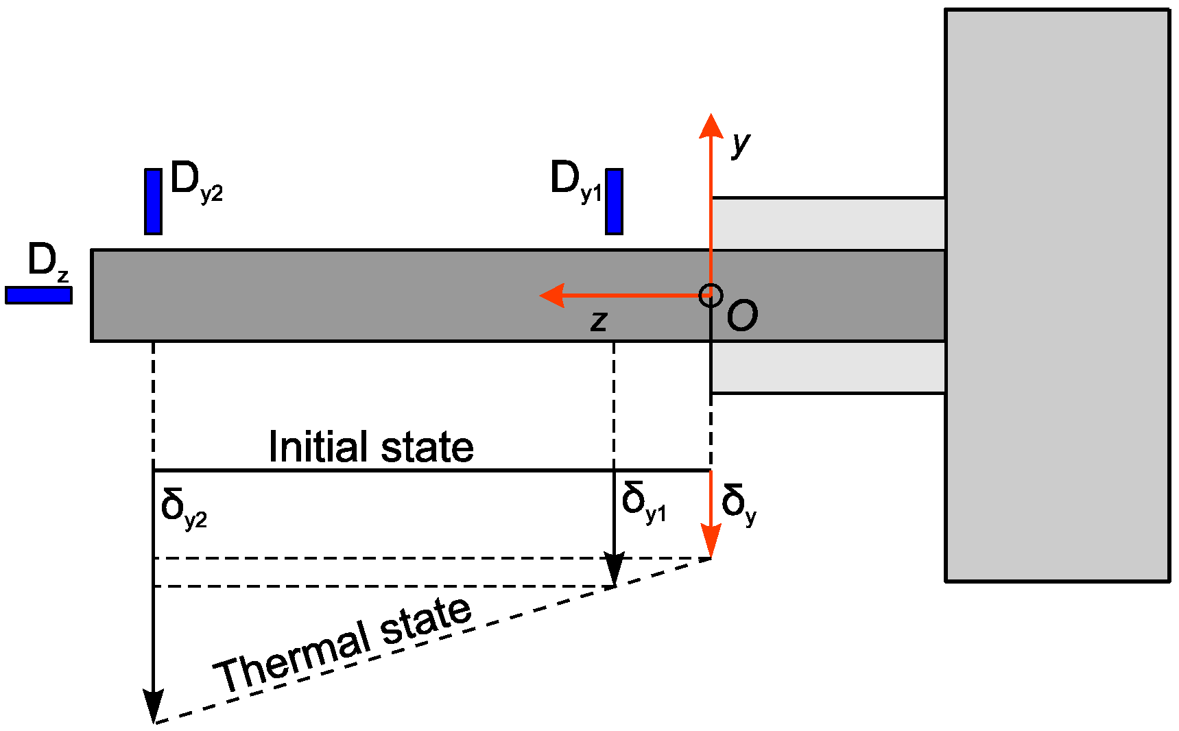
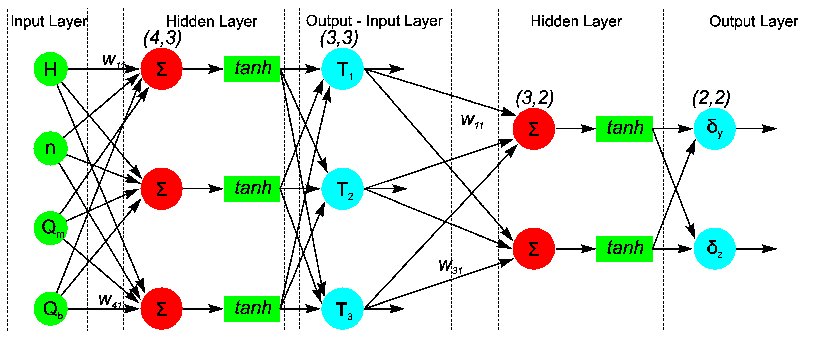
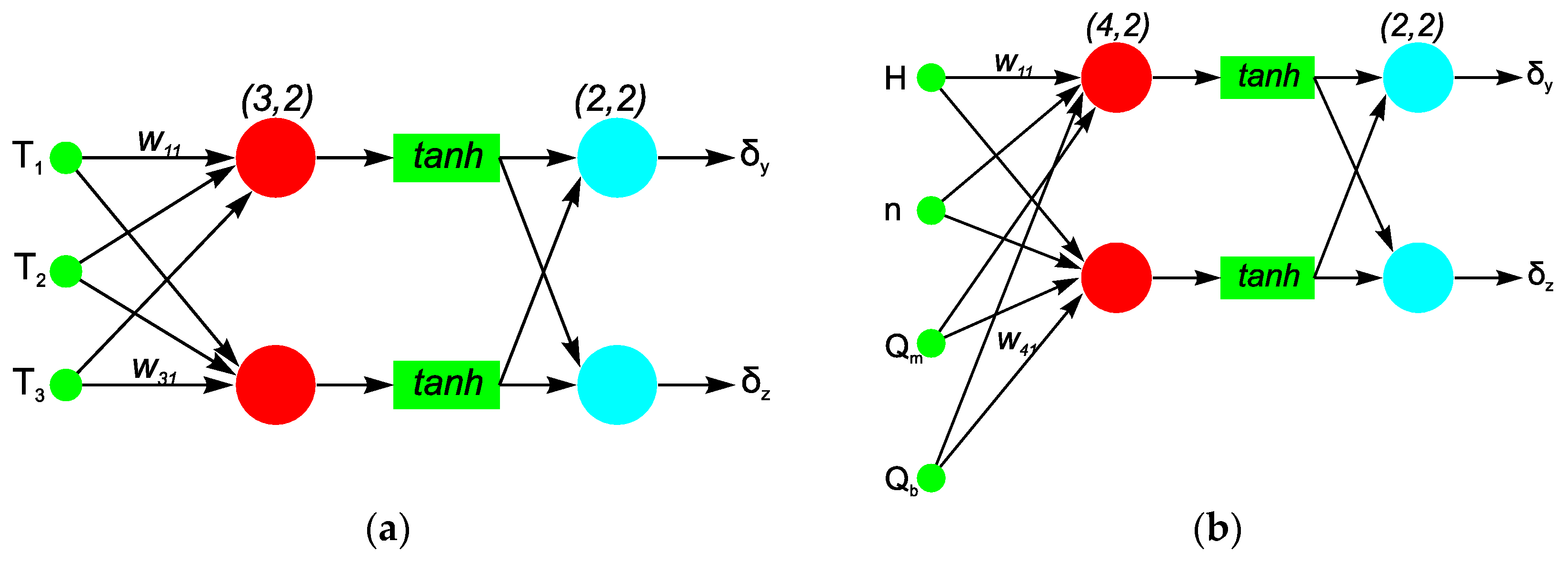
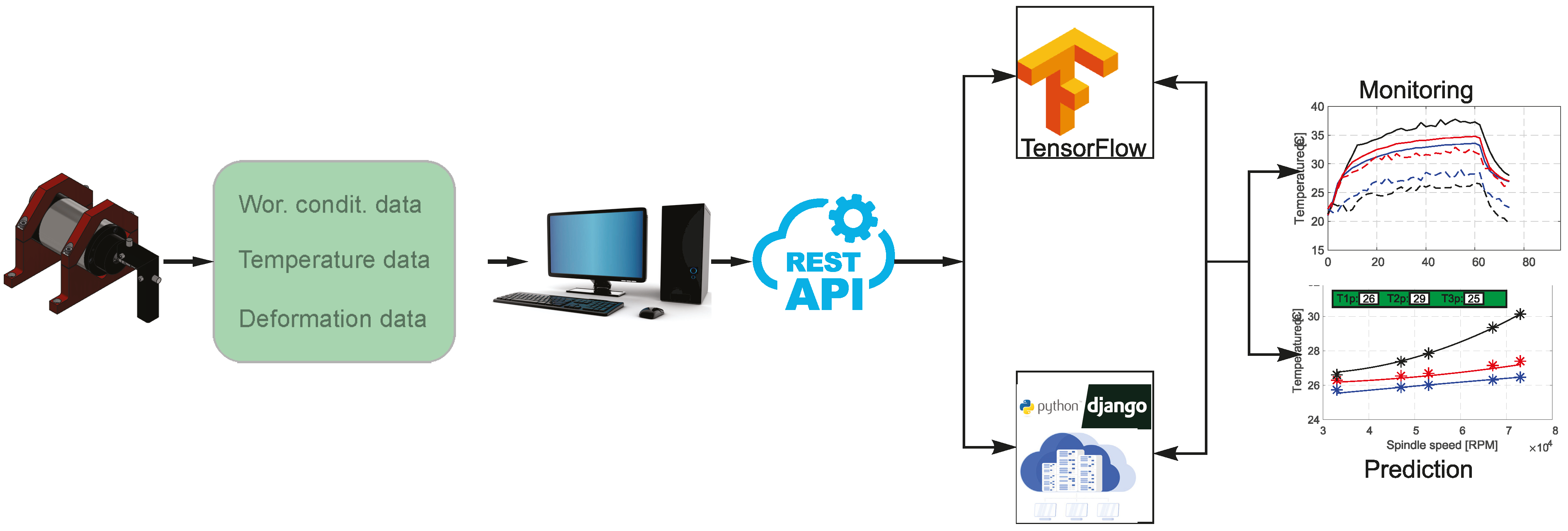
In this paper, experimental testing was conducted by utilizing an acquisition system to capture temperature and thermal deformation data across various spindle speeds, coolant types (oil, water), and coolant flow rates in the motor and bearings, representing different working conditions. Multiple Regression (MR) analysis is employed to delineate the relationships between input parameters (working conditions) and output parameters (temperatures), as well as temperature variables (input) and thermal deformation (output). Subsequently, comprehensive Multiple-Input Multiple-Output (MIMO) backpropagation (BP) neural network models are developed for predicting spindle temperature and thermal deformation, respectively. The models leverage working conditions as input parameters to predict temperatures and thermal deformations on the high-speed motorized spindle unit. Moreover, a novel system architecture incorporating cloud computing is introduced. Cloud Computing provides the opportunity to connect an unlimited number of geographically distributed setups to the same cloud system, which eliminates the necessity to train models or calculate predictions locally. Leveraging REST API calls, the system seamlessly uploads data and retrieves calculated predictions, therefore enhancing computational efficiency and scalability.

2. Defining Prediction Model

The paper focuses on a high-speed motorized spindle unit of grinding machine tools. Thermal equilibrium experiments were realized using an acquisition system to measure temperature and thermal deformations for different spindle speeds, coolant types (oil, water), and coolant flow of motor and bearings (working conditions). Choosing both coolant types enables a more thorough analysis of the algorithm’s performance and its sensitivity to variations in cooling conditions, contributing to a more profound understanding of its capabilities and limitations. We have assessed their effectiveness in cooling the system and determined which is more suitable for the specific application. The framework of the proposed model is shown in Figure 1. Upon gathering data, we analyzed the impact of various working conditions on spindle temperature and examined how these temperatures influence thermal deformation. Multiple Regressions (MRs) are used to establish the relationships between working conditions (input parameters) and temperatures (output parameters), as well as temperature variables (input parameters) and thermal deformations (output parameters). Working conditions were used as input parameters of the first ANN model (NNet1), while temperatures of the spindle unit were given as the output parameters. Subsequently, these temperatures are used as input parameters for the second ANN model (NNet2), employing thermal deformations on the spindle nose as output parameters. After successful separate training of NNet1 and NNet2 models, the models have been evaluated in sequence, i.e., normalized values of outputs obtained from NNet1 have been used as inputs to the previously trained NNet2 in the validation phase. Finally, comprehensive MIMO BP neural network (NNet) approaches were established for spindle temperature and thermal deformation. After the network learning and training, the temperatures and thermal deformation of the motorized spindle unit in multiple places have been accurately fitted and predicted. Furthermore, a system architecture involving cloud computing is developed. The models were migrated to a dedicated cloud solution developed for this purpose, wherein all calculations regarding predictions are conducted. This architecture relies on the REST API calls for uploading data and getting calculated predictions. Afterward, a new set of stochastic sample data is used to validate the model. The results indicate that the model exhibits a high level of prediction accuracy. This implies that an accurate model can be obtained, offering references for characteristic parameters related to thermal equilibrium.

3. Experimental Setup and Equipment

3.1. Experimental System

The experimental system is shown in Figure 2, which focuses on the high-speed motorized spindle unit (GMN TSSV 100-90000) of grinding machine tools. The spindle is mounted with two pairs of high-precision angular contact bearings, the front bearing with EX 12 7C1 DUL SNFA, and the rear bearing with EX 10 7C1 DUL SNFA, mounted in a “tandem” arrangement. The front bearings are equipped with a lock-ring preload, whereas the rear bearings have a constant preload. The test system consists of the speed control system (frequency regulator Nidec HS 72) of the motorized spindle, a cooling system, a system for measurement of fluid flow, and a data acquisition system. The maximum number of revolutions is n = 90,000 RPM. The cooling system consists of the motorized spindle stator cooling system and the bearing air–oil cooling system. Cooling and oil–air lubrication were performed by injecting oil Q_b = 0.18–0.24 L/h (permissible limits for the type of bearing used) for all bearings simultaneously.

Oil and water were utilized for cooling the spindle stator. The tank was cooled through a heat exchanger, maintaining a constant temperature for the oil or water in the tank at 22 °C. The oil or water temperature at the exit of the stator cooling jacket ranged between 23 and 28 °C, depending on input parameters. Oil or water flows through the groove around the stator with a flow rate of Q_m = 4–8 L/min. The system for measurement of fluid flow is composed of the Acrylic Flow Meters 6A01, measuring the amount of oil mist on the bearings at all times, and an Integral Flowmeter AXF, measuring the flow of the cooling fluid for the spindle stator.

The measuring equipment is used to determine the temperature and thermal deformation. To measure the temperature of the spindle unit, K-type thermocouples with an accuracy of ±0.2 °C at 100 °C, and a thermal imager with an accuracy of ±1% have been used. An infrared thermometer with an accuracy of ±0.2% has been used to record the temperature at the outlet coolant from the spindle unit. Edge current sensors (HBM) were applied to measure the thermal deformation. The diameter of the sensor head was 3 mm, and the degree of nonlinearity was 0.1%. The system achieves real-time synchronous acquisition of the temperature and thermal deformation by utilizing an NI USB 6281 acquisition system. The installation locations of the sensors and thermocouples are shown in Figure 3 and

Table 1. Measurements temperature location.

A Method of Measurement	Temperature	Location
Thermocouples, thermal imager	T1	near outer ring of front bearing
Thermocouples, thermal imager	T2	near stator of spindle
Thermocouples, thermal imager	T3	near outer ring of rear bearing
Thermal imager	T4	between front bearing and stator
Thermal imager	T4	between rear bearing and stator
Thermal imager, infrared thermometer	T0	at the outlet coolant from the spindle unit.

.

3.2. Measuring Principle of Thermal Deformation

The spindle thermal deformation is measured by using eddy current displacement sensors. After the spindle reaches a steady state, the thermal deformation expands to the axial and radial direction, resulting from the uneven temperature gradient distribution, which is shown in Figure 4. Also, in Figure 4, a measurement diagram of the thermal deformation of the spindle inspection bar is presented. The spindle is oriented along the Z-axis, so the axial thermal expansion can be obtained by measurement via the sensor D_z. The radial deformation in the Y direction is measured by the sensors D_y1 and D_y2. Based on these detections, spindle thermal errors are calculated according to the presented geometry relationship as specified in [33].

3.3. Results of the Experimental Testing and Analysis

Using the experimental setup described above, the motorized spindle unit operated under different working conditions. For the proposed experiments, the motorized spindle unit operated within the range of 20,000 to 80,000 RPM. The spindle speed influences the temperature field distribution and the value of thermal deformations. To simulate the actual working conditions changes during processing, flow rate fluids for cooling of the spindle stator (Q_m = 4; 6 and 8 L/min) and bearing (Q_b = 0.18; 0.21 and 0.24 L/h) varied during the experiment. Oil and water were used to cool the spindle stator. Based on the presented working condition parameters, 234 different experiments were performed, i.e., 234 sample data were generated for the neural network. The ambient temperature ranged from 20 to 22 °C. The acquisition system recorded the data once every 10 min. The specific distribution of working condition parameters is shown in Figure 5.

3.3.1. Temperature Fields Distribution

Figure 6 illustrates the temperature field of the spindle system in a stationary state. The temperature distribution within the spindle unit is nonuniform. As the rotor rotates with the spindle shaft, the heat is transferred from the rotor to the shaft and housing. Subsequently, the heat conducts along the shaft and bearings to the housing. Conversely, the heat from the stator is conducted to the bearings and housing. These processes collectively result in a pronounced temperature gradient along the axial and radial direction of the housing. The maximum temperature near the stator reaches 36.1 °C for the oil cooling spindle stator and 25.9 °C for the water cooling spindle stator, and the evident temperature gradient is attributed to the outer wall of the stator being in contact with the cooling water jacket. Despite the efficiency of the cooling system in dissipating a significant amount of the stator’s heat, the temperature of the stator remains higher than that of other components. When employing water cooling for the housing, a substantial amount of heat is transferred through water. Water-based cooling is typically more efficient, primarily attributed to its higher specific heat capacity (41.2 kJ/(kgK) at 20 °C for water, compared to 1.9 kJ/(kgK) for the specialized cooling oil). The maximum temperature near the front bearing reaches up to 35 °C for the oil cooling spindle stator and 23.5 °C for the water cooling spindle stator, whereas the maximum temperature near the rear bearings reaches up to 32 °C and 23 °C for oil and water cooling spindle stator.

The spindle unit temperature variations are shown in Figure 7. The temperatures of both the front and rear bearings exhibit a gradual increase from the outset, followed by a sudden rise in the early stage. Subsequently, they gradually stabilize towards the thermal equilibrium temperature, indicating a balance between the heat generation and dissipation into the atmosphere.

Furthermore, during the period when thermal equilibrium is not yet achieved, the temperatures undergo real-time dynamic changes. Experimental data show fluctuations (especially for water cooling) near the thermal stationary state, and these fluctuations are primarily attributed to the performance of the cooling system. During the cooling process, the front bearing, rear bearing, and the motor undergo separate cooling procedures. However, temperatures are restrained from rising significantly, as the cooling fluid removes an amount of heat energy that is less than the heat generated by the spindle motor. Consequently, the overall trend remains an increase in temperature. The temperatures at all measuring points generally rise over time, yet this overall increase exhibits cyclical changes with a recurring time cycle.

In Figure 8, the thermal stationary state temperatures of the spindle system’s key components are presented at various rotational speeds. The temperatures of these key components show an increase corresponding to the rotational speed, with the stator and bearings. These elements register higher temperatures compared to other components.

Figure 9 depicts the temperature rise as a function of the flow rate, Q_m, at a spindle speed of n = 80,000 RPM. The temperature gradient ΔT₂ exhibits its most notable increase at the minimum flow rate, Q_m = 4 L/min, peaking at ΔT₂ = 24.1 °C and 8.9 °C, depending on the cooling type. Subsequently, a slight decrease is observed at Q_m = 6 L/min, with ΔT₂ values of 22.2 °C and 5.8 °C, respectively. The smallest increase in temperature gradient occurs at Q_m = 8 L/min, yielding ΔT₂ values of 20.1 °C for oil cooling and 4 °C for water cooling. Based on these observations, it can be inferred that both the flow rate and the type of cooling fluid exert influence on the temperature distribution, whereby an increase in flow rate correlates with a decrease in maximum temperature.

3.3.2. Thermal Deformation

The test results for the motorized spindle are presented in Figure 10. When the thermal deformation reaches over 90% of its maximum value, it is considered to be in a steady state. It can be observed that the time taken to reach the thermal steady state was consistently around 10 to 15 min for various rotational speeds. The trend of the thermal deformation initially increased rapidly, then slowed down, and eventually stabilized. The periodic fluctuation in the thermal deformation, as shown in the figures, was caused by variations in the cooling oil and water temperature.

Table 2. Thermal deformation in stationary state at different spindle speeds.

RPM	Steady-State Thermal Deformation Values in [μm]
	Oil Cooling		Water Cooling
	δz	δy	δz	δy
50,000	1.61	−1.94	1.58	−1.71
60,000	1.77	−2.31	1.68	−2.29
70,000	2.15	−2.57	1.97	−2.41
80,000	2.46	−3.51	2.26	−2.96

illustrates the thermal deformation values when the motorized spindle reached a steady state for different rotational speeds. Based on the provided diagrams (Figure 10) and data from Table 2, it is evident that variations in flow rate have a discernible impact on spindle deformation. Specifically, in the radial direction (vertical plane), at a spindle speed of n = 80,000 RPM, deformations at Q_m = 4 [L/min] are notably 10 [%] to 13 [%] larger compared to those at Q_m = 8 [L/min]. Furthermore, the choice of cooling medium significantly influences the spindle deformations. When water is used to cool the housing, axial and radial deformations are consistently reduced by 8 [%] to 18 [%] and 6 [%] to 15 [%], respectively, in comparison to cooling with oil.

3.4. Selection of Input Variables

A multitude of input parameters can negatively impact the prediction accuracy and quality of a thermal prediction model. The machine tool’s spindle can be compensated with the temperature that correlates with the temperature of the working conditions (such as the spindle speeds, type of coolant, and coolant flow of motor and bearings). Also, the spindle can be compensated with thermal deformations that correlate with thermal deformations of the temperature variables. A multiple regression is applied in this paper to assess the association between two or more independent variables and a single continuous dependent variable. The multiple regression equation for assessing the association between working conditions (spindle speeds, type of coolant, and coolant flow of motor and bearings) and temperature is expressed as

$$T_i={\beta }_0+{\beta }_{1}n+{\beta }_2{Q}_m+{\beta }_3{Q}_l+{\beta }_1{n}^2\dots +{\beta }_i{Q}_m{Q}_l+\epsilon ; i=1,2,3,\dots n$$

(1)

where T_i is the temperature; n, Q_m, and Q_l are changes in the input parameters: spindle speeds and coolant flow of the spindle stator and bearings, respectively; β represents regression coefficients, which is a p-dimensional parameter vector; ε is residual. The previous relation is valid for both types (oil and water) of spindle stator cooling. A special experiment was carried out for “oil” and “water”. The experiment, as defined in this way, is divided into two blocks. The role of the blocks is to reduce or eliminate the variability caused by interference factors that may affect the response but are not directly related, as a design factor. The multiple linear regression equation to assess the association between temperatures and thermal deformation is given as:

$$\delta ={\beta }_0+{\beta }_1{T}_1+{\beta }_2{T}_2+\dots {\beta }_i{T}_i+\epsilon ; i=1,2\dots n$$

(2)

where T represents the change of the temperature variables. In the equations, i = 1, 2, …, n, are the temperature and thermal deformation measurement points. Correlation coefficients (p) are shown in

Table 3. Correlation coefficients (p) between input (working conditions) parameters and temperature.

Temperatures (output variables)	T1	0.018	0.022	0.025	0.015
	T2	0.010	0.015	0.012	0.061
	T3	0.021	0.021	0.023	0.016
	T4	0.064	0.081	0.056	0.095
	T5	0.063	0.081	0.059	0.096
	T0	0.051	0.091	0.024	0.099
		H	n	Qm	Qb
		Working conditions (input variables)

and

Table 4. Correlation coefficients (p) between input (temperatures) parameters and thermal deformation.

Thermal deformat. (out. variables)	δy	0.0010	0.00181	0.00281	1.2351	1.246	0.0785
	δz	0.0015	0.00185	0.00275	1.2422	1.268	0.0742
		T1	T2	T3	T4	T5	T0
		Temperatures (input variables)

. According to the ANOVA method, all values of p < 0.05 indicate a significant mutual influence of the considered parameters.

Based on Table 3, it can be seen that the considered working conditions, to a greater or lesser extent, affect the observed temperatures of the main spindle. So, the temperatures T₄ and T₅ mostly depend on the amount of heat transfer from the stator and bearing and the construction of the spindle. Therefore, it can be concluded that working conditions indirectly affect these temperatures, but to a lesser extent than temperatures T₁, T_2, and T₃. T₀ is the outlet temperature of the spindle stator coolant, and its temperature depends on coolant flow and the heat generated into the spindle. The comprehensive correlation between the temperature and output variables can be expressed by correlation coefficients given in Table 4.

Table 4 shows a correlation coefficient (p) for all input variables. The correlation between outputs and input variables T₁, T₂, and T₃ indicates that they are strongly correlated. The correlation between output variables and input variable T₀ has values of 0.074 and 0.078. That indicates the presence of correlation, but not as significant as in the previous case. The correlation between output variables and input variables T₄ and T₅ is negligible, indicating that the relationship is not noticeable. Bearing those facts, T₁, T₂, and T₃ are chosen as the typical temperature variables.

4. MIMO Neural Network Models

A multi-input multi-output spindle thermal model was created using a simple feed-forward neural network with backpropagation (BP). Neurons serve as the fundamental components of a neural network. Based on their characteristics and functions, neurons function as nonlinear information processing units with the capability of handling multiple inputs and generating multiple outputs. Numerous neurons with similar structures are interconnected to compose the network structure. Considering the number of training samples in our dataset as well as the complexity of input and output training data, three different neural network architectures have been proposed. After the comprehensive testing, the proposed models were connected into one complex model.

4.1. Temperature Modelling Based on MIMO BP Neural Network

Let us consider the input to the BP neural network (BPNN) as W_i(n, Q_m, Q_b, H), representing variables related to working conditions. Let us also denote the output of the BPNN as Temp, representing the temperatures. If w_ij(i = 1, 2, 3, 4; j = 1, 2, 3) denotes the weights between the input layer and the hidden layer, ϕ_j(j = 1, 2, 3) denotes the biases of hidden nodes, T_j(j = 1, 2, 3) denotes the weights between the hidden layer and the output layer, and θ represents the bias of the output node, the computational procedure for determining the temperatures can be expressed as follows:

$$\begin{gathered} I_i={\displaystyle \sum _{j=1}^3{w}_{ij}{W}_i+{\varphi }_j} \\ \begin{array}{l}{O}_i=f(I_i)\hspace{1em}\hspace{1em}\hspace{1em}1\le i\le 4\\ Temp={\displaystyle \sum _{j=1}^3{T}_j{O}_i+\theta }\end{array} \end{gathered}$$

(3)

The first neural network (denoted as NNet1) (depicted in Figure 11) is designed to capture the relationship between the working conditions—specifically, the spindle speed n (given in revolution per minute—RPM), the coolant type H (represented in a binary form as 0 and 1 for oil and water, respectively), the coolant flow of the motor Q_m [L/min], and the coolant flow of the bearings Q_b [L/h], versus the output temperatures T₁, T₂ and T₃ [°C], acquired through experimental testing. All input values have been normalized to the [0, 1] range. The network consists of one input (4,3) layer, one output (3,3) layer, and a hyperbolic tangent (tanh) layer between them (the numbers in brackets represent the number of inputs and the number of neurons, i.e., the outputs).

4.2. Thermal Deformation Modelling Based on MIMO BP Neural Network

The second neural network model (denoted as NNet2) retains a similar structure, containing one input (3,2) and one output (2,2) linear layer, and a hyperbolic tangent layer between them, modeling the connection between the normalized values of temperatures T₁, T_2, and T₃, and thermal deformations of the motorized spindle unit obtained by experimental testing, δ_y and δ_z. The third neural network model (denoted as NNet3) establishes the relationship between the input parameters {n, H, Q_m, Q_b} and the resulting thermal deformations {δ_z, δ_y} directly, using two linear layers with sizes (4,2) and (2,2) and a hyperbolic tangent layer positioned between them. The dimensions of these layers correspond to the input and output network parameters. This model functioned as a control and monitoring framework. The architectures of the proposed neural network models modeling thermal deformations are illustrated in Figure 12.

In our experiments, all networks were trained using a Stochastic Gradient Descent (SGD) optimizer, with a learning rate set to 0.1, and the L1 loss criterion, measuring the mean absolute error (MAE) between the predicted and measured data as:

$$\begin{array}{l}L{1}_{lf}={\displaystyle \sum _{i=1}^m\left|Y_{exp}-Y_{pred}\right|}\\ MAE=\frac{L{1}_{lf}}{m}\end{array}$$

(4)

Following the successful individual training of NNet1, NNet2, and NNet3 models, the models have been evaluated in sequence. Specifically, the normalized values of outputs obtained from NNet1 have been used as inputs to the previously trained NNet2 in the validation phase, i.e.,:

NNnet. = NNet2[NNet1((n, H, Qm, Qb))norm.]

(5)

The architectures of the proposed neural network models for predicting and monitoring thermal elastic behavior are presented in Figure 13.

4.3. Evaluation of BP Neural Network Models

NNet1, NNet2, and NNet3 models underwent training over 200 epochs, a duration determined through observation of error rates during the validation phase to optimize the results and mitigate overfitting. A total of 234 samples {n, H, Q_m, Q_b, T₁, T₂, T₃, δ_y, δ_z} were employed, i.e., 200 samples within a 1-fold training scenario, while the remaining 34 samples were set aside for validation purposes. Figure 14a represents the results for NNet1, focusing on validation loss, calculated as the average discrepancy (L1 norm) between the predicted and measured temperature values (T₁, T₂, and T₃) for the final epoch of each fold. The mean error value, encompassing all outliers, was 1.48 °C. Similarly, in Figure 14b, the results obtained for NNet2 are depicted following a parallel training approach. NNet2 employed normalized temperature values from areas adjacent to the front and rear bearings, as well as the stator of the motor (T₁, T₂, T₃), as inputs, while the previously determined thermal deformations {δ_y, δ_z} were designated as output values. The mean error value was 0.10 µm. Finally, in Figure 14c, the results obtained for NNet3 are showcased. The model underwent training using normalized input parameters {n, H, Q_m, Q_b}, utilizing thermal deformations {δ_y, δ_z} as outputs. The mean error value was determined to be 0.20 µm.

Following individual training of NNet1, NNet2, and NNet3 models, a sequential evaluation was carried out, wherein the normalized outputs from NNet1 were employed as inputs for the previously trained NNet2 during the validation phase, i.e., NNet. = NNet2(NNet1({n, H, Q_m, Q_b})_norm). The outcomes, illustrated in Figure 14d, indicated a reduced error rate of 0.08 µm, using 34 training samples that were not seen by NNet1 and NNet2 models during the training phase.

5. Cloud Computing

After the offline development of the model for predicting temperature and thermal deformations, the calculation of predictions was moved to a cloud computing system. For this purpose, a web application that is based on the Python Django web framework that implements desired model calculations is developed. REST API was used to upload input data and obtain model outputs in the response. The architecture of this part of the proposed solutions is given in Figure 15. The architecture ensures that predicting temperature and thermal deformations is not only locally available but can be used no matter where setup and equipment are mounted as far as the setup is connected to the internet. Connection between the cloud platform and the physical model is established through the PC that serves as a gateway. The gateway captures the real-time data of equipment workload, working conditions (spindle speeds, type of coolant (oil, water), and coolant flow of motor and bearings), spindle temperature, and thermal deformations from the physical equipment. The data are preprocessed and sent to the cloud platform where spindle temperature or deformation is predicted, which is later used on the gateway to adapt working conditions. The preprocessed data are encapsulated in a JavaScript Object Notation (JSON) format. Mainly, the gateway is used to acquire the working conditions data (spindle speeds, type of coolant (oil, water), and coolant flow of motor and bearings) and sensor data (spindle temperature and thermal deformations) of experimental equipment using different communication and acquisition interfaces (i.e., Modbus, OPC DA, and NI Acquisition Cards). The PC gateway then makes local analysis, preprocessing this data and formatting it into an adequate object that is sent to the cloud platform.

6. System Validation

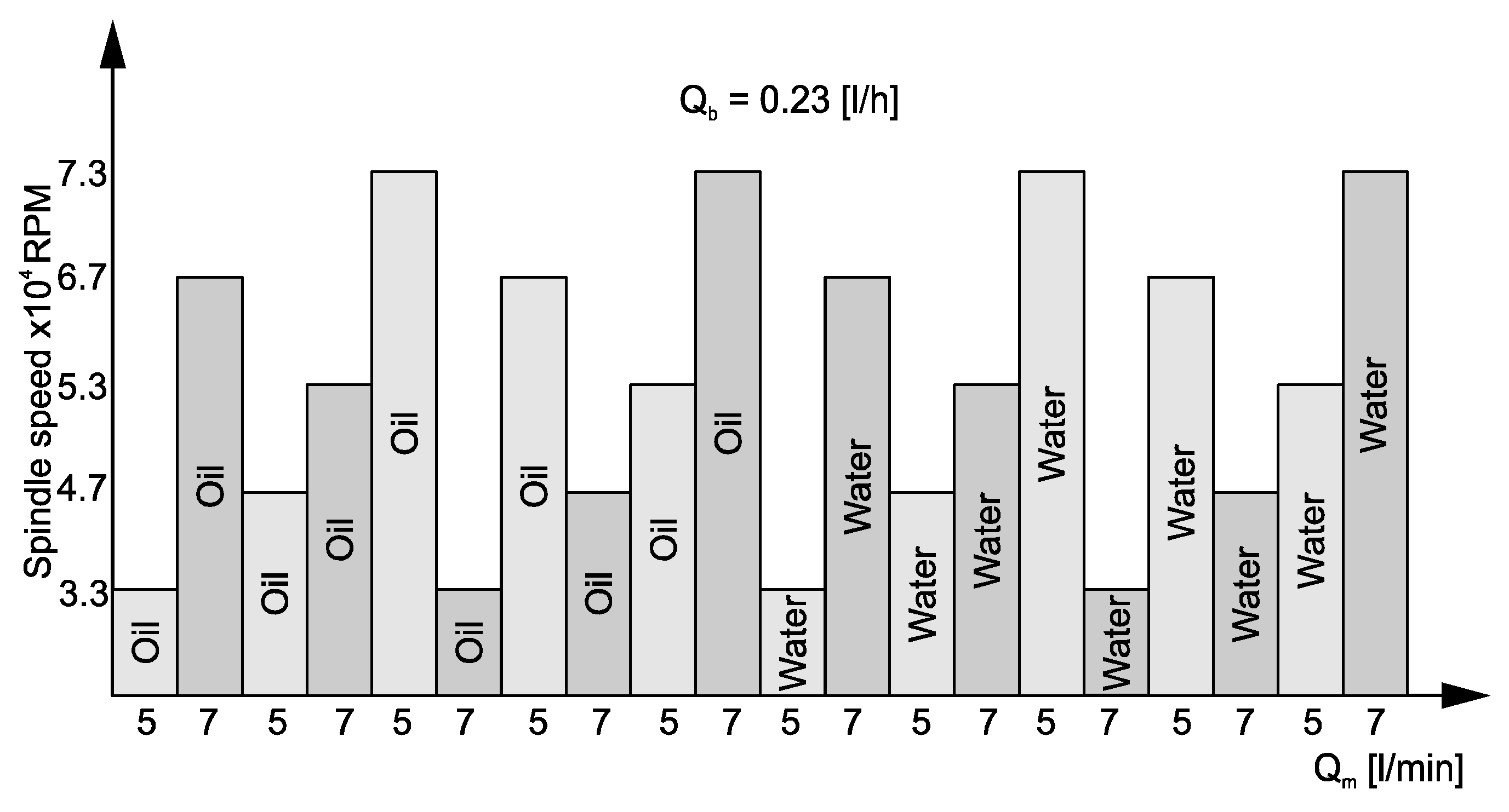
Following the offline development of the temperature and thermal deformation prediction model, the computation of forecasts was transitioned to a cloud computing system where monitoring and forecasting of temperatures and thermal deformations were carried out. A comparison with the results of experimental tests is presented below. To ascertain the model’s validity, newly acquired data samples (20 samples in total) were employed to predict spindle thermal behavior. 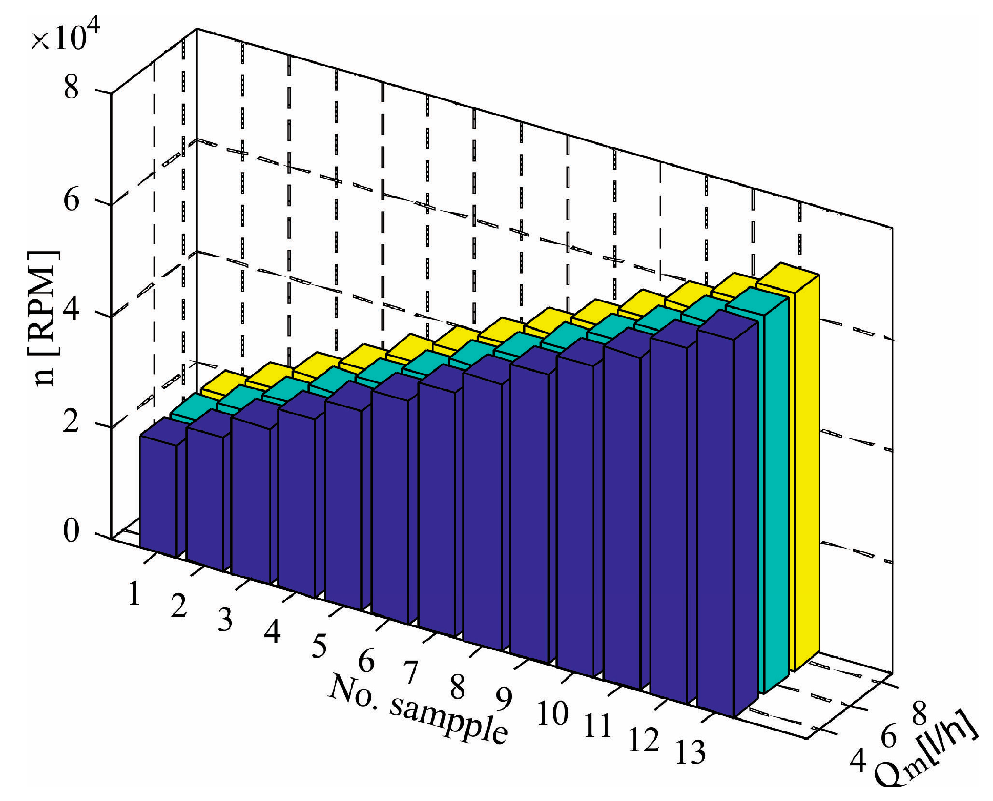Figure 16 illustrates the spindle speeds and flow rate map corresponding to these data samples.

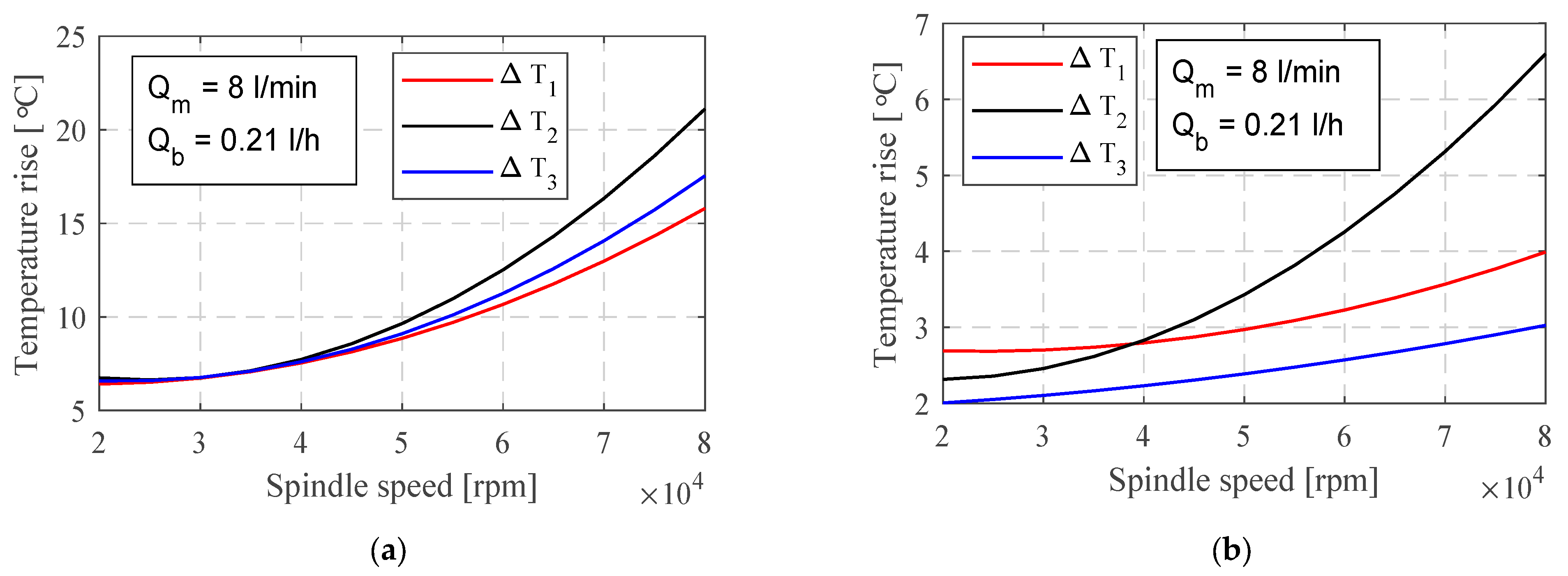
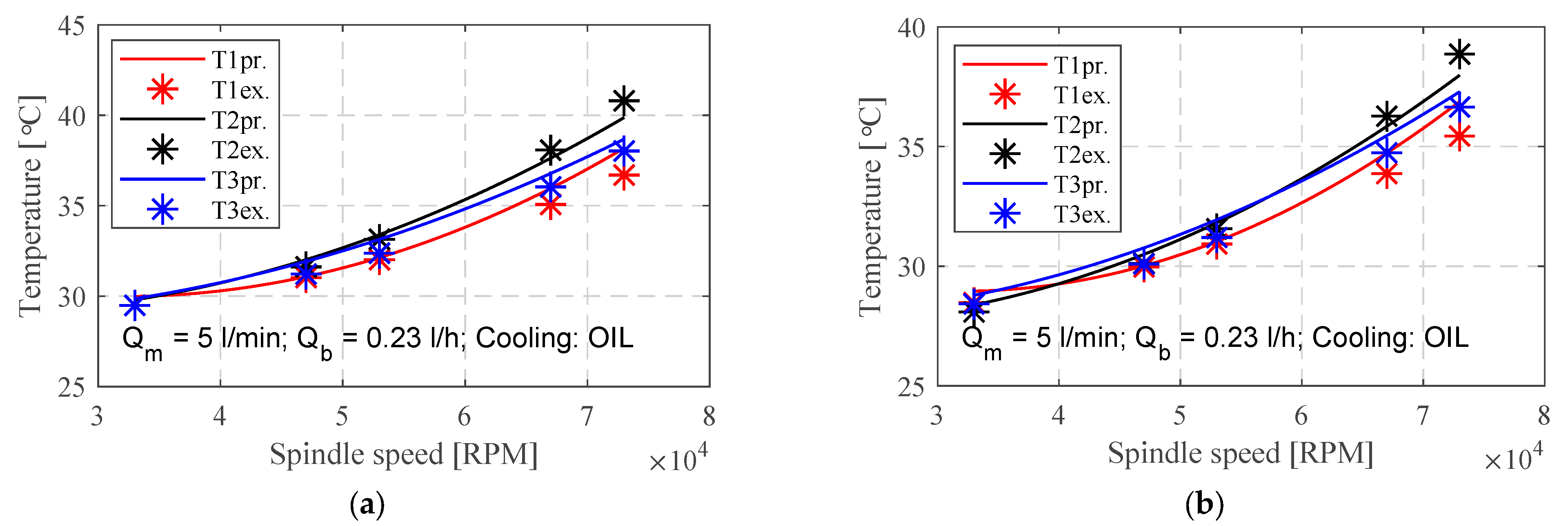
The comparison between the temperature results predicted by the model and the experimental data for cooling the spindle stator with oil and water are shown in Figure 17 and Figure 18. Figure 17 illustrates temperature variations corresponding to different oil flow rates (Q_m) through the housing as a function of the spindle’s revolutions. Elevating the spindle speed from 33,000 to 73,000 RPM resulted in a temperature rise of 38% at an oil flow of Q_m = 5 L/min according to experimental testing, and a 35% increase is predicted by the model. Similarly, for an oil flow of 7 L/min, experimental testing shows a temperature increase of 35%, while the prediction model indicates a 33% rise. Conversely, increasing the flow from 5 to 7 L/min induces a temperature decrease of approximately 3% at n = 33,000 RPM or 5% at n = 70,000 RPM for T₁ and T₃, according to experimental results, and 1% and 3%, respectively, as per the prediction model. Regarding T₂, a reduction of 2% at n = 33,000 RPM and 8% at n = 73,000 RPM is observed in experimental testing, whereas the prediction model anticipates a decrease of 6%. The residual temperature spans from 0.05 to 1.87 °C, depending on oil flows and spindle speed.

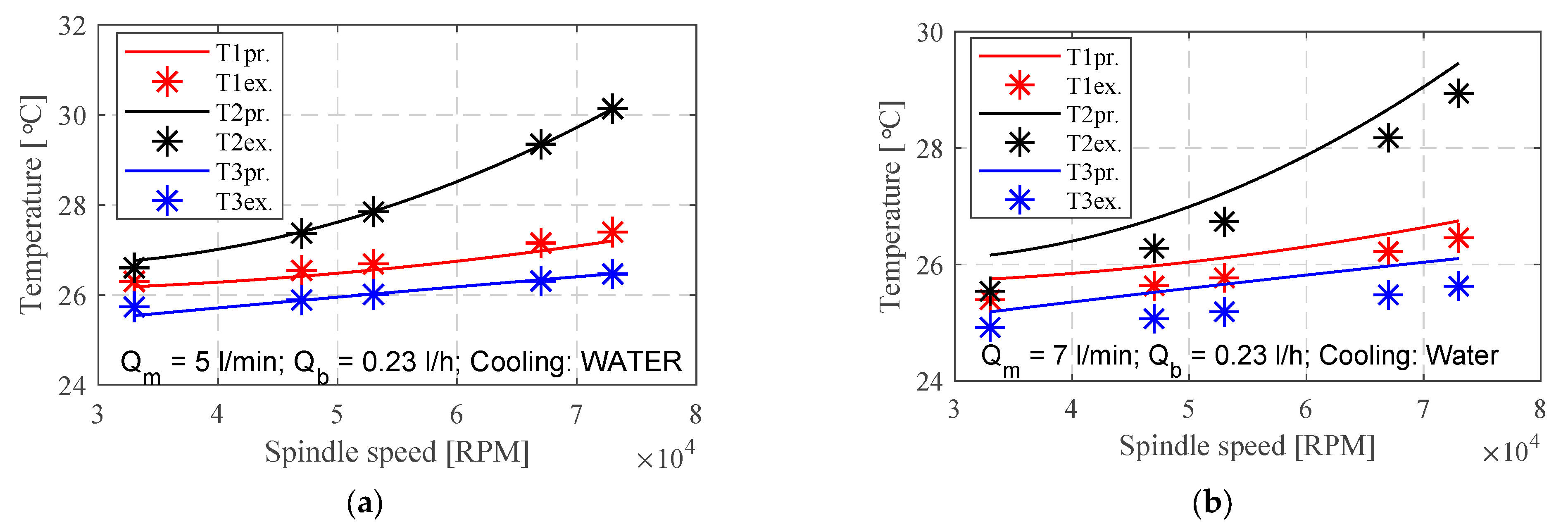
Temperature variations concerning different water flow rates (Q_m) through the housing in relation to the spindle’s revolutions are illustrated in Figure 18. Increasing the spindle speed from 33,000 to 73,000 RPM produced a temperature rise of 13% at an oil flow of Q_m = 5 L/min according to experimental testing and 12% based on the prediction model. At a flow of 7 L/min, experimental testing shows a temperature increase of 10%, while the prediction model indicates an 8% rise. Conversely, augmenting the flow from 5 to 7 L/min results in a temperature decrease of approximately 3% at n = 33,000 RPM or 4% at n = 73,000 RPM for T₁ and T₃, as observed through experimental testing. According to the prediction model, the corresponding decreases are 2% and 3%, respectively. Regarding T₂, a decrease of 4% at n = 33,000 RPM and 10% at n = 73,000 RPM is observed through experimental testing, while the prediction model predicts a decrease of 9%. The residual temperature ranges from 0.03 to 0.61 °C, depending on water flows and spindle speed. The predictive model provides R-squared values ranging from R² = 0.95 to 0.98, which can be considered as good for all temperature outputs.

The comparison between the thermal deformation predicted by the model and the experimental data at different speeds, cooling types and flow are shown in

Table 5. Thermal deformation predicted by the model and the experimental data for cooling the spindle stator with oil at Q_m = 5 L/min.

Spindle Speed RPM	Measurements Data		Predictions Data		Error
	|δy|	δz	|δy|	δz	|δy|	|δz|
33,000	1.28	1.06	1.37	0.98	0.09	0.08
47,000	1.82	1.42	1.93	1.31	0.11	0.11
53,000	2.04	1.56	2.22	1.49	0.18	0.07
67,000	2.46	2.06	2.83	1.96	0.37	0.10
73,000	3.20	2.24	3.29	2.13	0.09	0.11

,

Table 6. Thermal deformation predicted by the model and the experimental data for cooling the spindle stator with oil at Q_m = 7 L/min.

Spindle Speed RPM	Measurements Data		Predictions Data		Error
	|δy|	δz	|δy|	δz	|δy|	|δz|
33,000	1.21	1.01	1.12	0.99	0.09	0.02
47,000	1.44	1.19	1.54	1.41	0.10	0.22
53,000	1.66	1.27	1.72	1.59	0.06	0.31
67,000	2.04	1.71	2.14	2.01	0.10	0.30
73,000	2.54	2.13	2.32	2.19	0.22	0.06

,

Table 7. Thermal deformation predicted by the model and the experimental data for cooling the spindle stator with water at Q_m = 5 L/min.

Spindle Speed RPM	Measurements Data		Predictions Data		Error
	|δy|	δz	|δy|	δz	|δy|	|δz|
33,000	1.13	1.04	1.21	1.13	0.08	0.09
47,000	1.61	1.42	1.77	1.55	0.16	0.13
53,000	2.02	1.48	2.01	1.73	0.01	0.25
67,000	2.31	1.89	2.57	2.15	0.26	0.27
73,000	2.70	2.06	2.81	2.33	0.11	0.27

and

Table 8. Thermal deformation predicted by the model and the experimental data for cooling the spindle stator with water at Q_m = 7 L/min.

Spindle Speed RPM	Measurements Data		Predictions Data		Error
	|δy|	δz	|δy|	δz	|δy|	|δz|
33,000	1.04	0.97	1.13	0.75	0.15	0.21
47,000	1.24	1.19	1.35	1.03	0.20	0.15
53,000	1.60	1.18	1.78	1.15	0.05	0.02
67,000	1.87	1.53	2.24	1.43	0.32	0.09
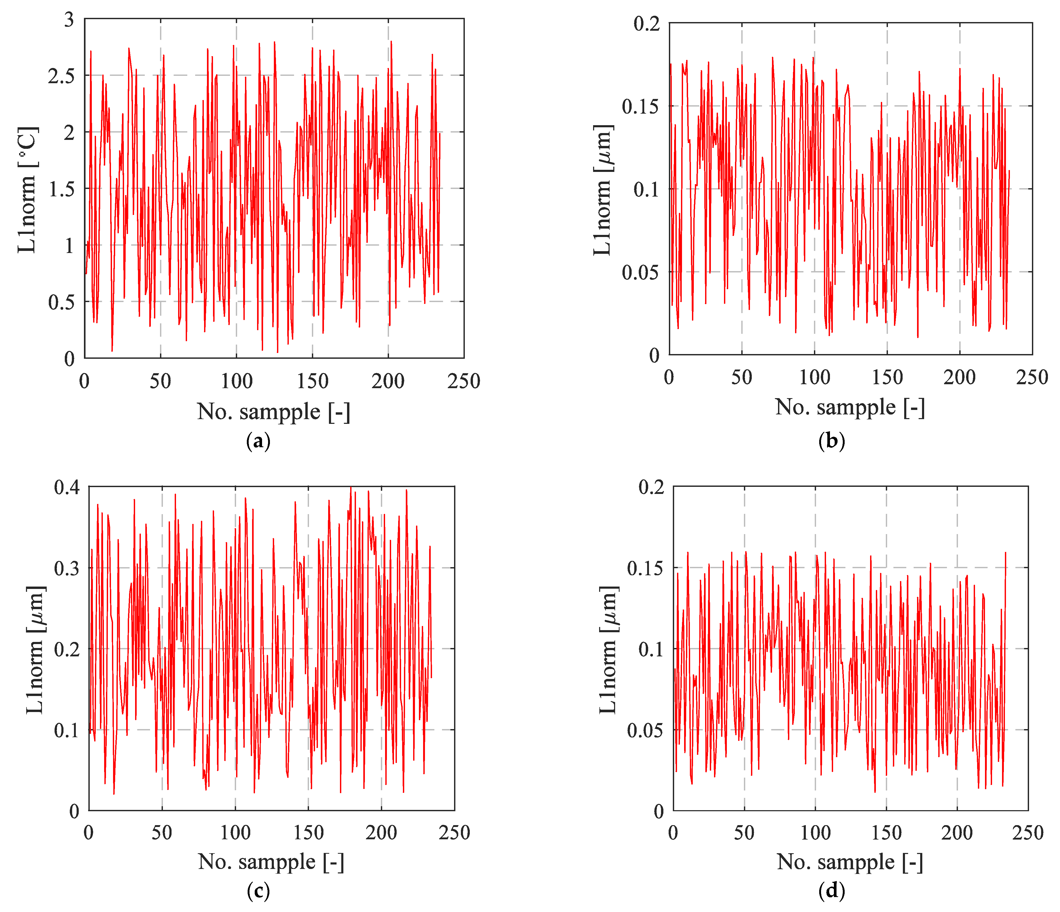
73,000	2.50	1.91	2.59	1.55	0.12	0.35

. The absolute values of the residuals for axial thermal deformation fall within the range of 0.02 to 0.35 [μm], while the radial thermal deformation residuals range from 0.01 to 0.37 [μm]. The average absolute values of the residuals for axial and radial thermal deformation are 0.16 and 0.14 [μm], respectively. Moreover, the predictive ability of the thermal deformation was 90% and 93%, indicating the model exhibits good predictive ability and perfect generalization. However, the average prediction error in the thermal deformation was approximately 0.3 μm.

The average coefficient of the determination, at 0.969, signifies that the ability of prediction is 96.9%, indicating that the four working conditions variables are robust and accurate predictors of the temperature and thermal deformation of the spindle unit. In a large number of previous papers, the average prediction accuracy was from 87 to 96% (most often around 95%).

The high coefficient of determination underscores the robustness and accuracy of the model in predicting spindle temperatures and thermal deformations under different working conditions. The comparison between simulated and measured results highlights the potential of this thermal model, based on artificial neural networks and cloud computing, to forecast spindle thermal behaviour in real time.

7. Conclusions

In summary, the transition of the temperature and thermal deformation prediction model to a cloud computing system has enabled efficient monitoring and forecasting of spindle temperatures and thermal deformations. Validation of the model was achieved through comparison with experimental tests, utilizing newly acquired data samples.

The comparison between predicted temperature results and experimental data for both oil and water cooling methods demonstrated close alignment, with residual temperatures within acceptable ranges. The predictive model exhibited strong performance, as evidenced by R-squared values ranging from 0.95 to 0.98, indicating good predictive accuracy for all temperature outputs.

Similarly, the comparison between predicted thermal deformations and experimental data showcased the model’s reliability, with low residual values and high predictive ability percentages. The average coefficient of determination further confirmed the robustness of the model, with a high prediction accuracy of 96.9%.

Based on these findings, insights into the historical temperature distribution of the motorized spindle unit can be gleaned, facilitating the selection of optimal coolant types and flow rates to mitigate temperature elevation and thermal expansion. The temperature results derived from the presented model enable the identification of optimal solutions and quantitative evaluation of enhancements in high-speed motorized spindle thermal characteristics. Selecting the suitable coolant and flow rate not only enhances the energy efficiency of the machine tool but also mitigates temperature fluctuations and errors stemming from heat load.

Overall, these findings suggest that the developed model, leveraging cloud computing and experimental validation, is an effective tool for predicting the temperature and thermal deformation of spindle units under various working conditions. This model holds promise for real-time monitoring and optimization of spindle performance, with potential applications in improving manufacturing processes and equipment reliability.

References

1. Li, Y.; Yu, M.; Bai, Y.; Hou, Z.; Wu, W. A Review of Thermal Error Modeling Methods for Machine Tools. Appl. Sci. 2021, 11, 5216. [Google Scholar] [CrossRef]
2. Ramesh, R.; Mannan, M.; Poo, A. Error compensation in machine tools—A review: Part II: Thermal errors. Int. J. Mach. Tools Manuf. 2000, 40, 1257–1284. [Google Scholar] [CrossRef]
3. Josef, M.; Jedrzejewski, J.; Uhlmann, E.; Donmez, M.A.; Knapp, W.; Härtig, F.; Wendt, K.; Moriwaki, T.; Shore, P.; Schmitt, R.; et al. Thermal Issues in Machine Tools. CIRP Ann. Manuf. Technol. 2012, 61, 771–791. [Google Scholar]
4. Cao, Y. Modeling of High-Speed Machine-Tool Spindle Systems. Ph.D. Thesis, University of British Columbia, Kelowna, BC, Canada, 2006. [Google Scholar]
5. Li, Z.; Yang, J.; Fan, K.; Zhang, Y. Integrated geometric and thermal error modeling and compensation for vertical machining centers. Int. J. Adv. Manuf. Technol. 2015, 76, 1139–1150. [Google Scholar] [CrossRef]
6. Naumann, C.; Riedel, I.; Ihlenfeldt, S.; Priber, U. Characteristic Diagram Based Correction Algorithms for the Thermo-elastic Deformation of Machine Tools. Procedia CIRP 2016, 41, 801–805. [Google Scholar] [CrossRef]
7. Chen, J.-S. A study of thermally induced machine tool errors in real cutting conditions. Int. J. Mach. Tools Manuf. 1996, 36, 1401–1411. [Google Scholar] [CrossRef]
8. Han, J.; Wang, L.; Wang, H.; Cheng, N. A New Thermal Error Modeling Method for Cnc Machine Tools. Int. J. Adv. Manuf. Technol. 2012, 62, 205–212. [Google Scholar] [CrossRef]
9. Shi, H.; Ma, C.; Yang, J.; Zhao, L.; Mei, X.; Gong, G. Investigation into effect of thermal expansion on thermally induced error of ball screw feed drive system of precision machine tools. Int. J. Mach. Tools Manuf. 2015, 97, 60–71. [Google Scholar] [CrossRef]
10. Zhang, J.; Li, B.; Zhou, C.; Zhao, W. Positioning error prediction and compensation of ball screw feed drive system with different mounting conditions. Proc. Inst. Mech. Eng. Part B J. Eng. Manuf. 2016, 230, 2307–2311. [Google Scholar] [CrossRef]
11. Hao, W.; Hongtao, Z.; Qianjian, G.; Xiushan, W.; Jianguo, Y. Thermal error optimization modeling and real-time compensation on a CNC turning center. J. Am. Acad. Dermatol. 2008, 207, 172–179. [Google Scholar] [CrossRef]
12. Huang, Y.; Zhang, J.; Li, X.; Tian, L. Thermal error modeling by integrating GA and BP algorithms for the high-speed spindle. Int. J. Adv. Manuf. Technol. 2014, 71, 1669–1675. [Google Scholar] [CrossRef]
13. Yang, J.; Shi, H.; Feng, B.; Zhao, L.; Ma, C.; Mei, X. Applying Neural Network based on Fuzzy Cluster Pre-processing to Thermal Error Modeling for Coordinate Boring Machine. Procedia CIRP 2014, 17, 698–703. [Google Scholar] [CrossRef]
14. Li, B.; Tian, X.; Zhang, M. Thermal error modeling of machine tool spindle based on the improved algorithm optimized BP neural network. Int. J. Adv. Manuf. Technol. 2019, 105, 1497–1505. [Google Scholar] [CrossRef]
15. Li, Z.; Zhu, B.; Dai, Y.; Zhu, W.; Wang, Q.; Wang, B. Research on Thermal Error Modeling of Motorized Spindle Based on BP Neural Network Optimized by Beetle Antennae Search Algorithm. Machines 2021, 9, 286. [Google Scholar] [CrossRef]
16. Lv, C.; Liu, Z.Y.; Liu, Z.J.; Yu, Z.M. Application of Generalized Radial Basis Function Neural Network to Thermal Error Modeling. Opt. Precis Eng. 2015, 23, 1705–1713. [Google Scholar]
17. Zhang, H.N. Research on Modeling of Machining Center Spindle Thermal Error Based on Improved Rbf Network. Tech. Autom. Appl. 2019, 38, 60–74. [Google Scholar]
18. Fu, G.; Gong, H.; Gao, H.; Gu, T.; Cao, Z. Integrated thermal error modeling of machine tool spindle using a chicken swarm optimization algorithm-based radial basic function neural network. Int. J. Adv. Manuf. Technol. 2019, 105, 2039–2055. [Google Scholar] [CrossRef]
19. Li, Z.; Zhu, B.; Dai, Y.; Zhu, W.; Wang, Q.; Wang, B. Thermal error modeling of motorized spindle based on Elman neural network optimized by sparrow search algorithm. Int. J. Adv. Manuf. Technol. 2022, 121, 349–366. [Google Scholar] [CrossRef]
20. Zhang, Y.; Yang, J.; Jiang, H. Machine tool thermal error modeling and prediction by grey neural network. Int. J. Adv. Manuf. Technol. 2012, 59, 1065–1072. [Google Scholar] [CrossRef]
21. Abdulshahed, A.M.; Longstaff, A.P.; Fletcher, S.; Potdar, A. Thermal error modelling of a gantry-type 5-axis machine tool using a Grey Neural Network Model. J. Manuf. Syst. 2016, 41, 130–142. [Google Scholar] [CrossRef]
22. Ma, C.; Zhao, L.; Mei, X.; Shi, H.; Yang, J. Thermal error compensation of high-speed spindle system based on a modified BP neural network. Int. J. Adv. Manuf. Technol. 2017, 89, 3071–3085. [Google Scholar] [CrossRef]
23. Guo, Q.; Xu, R.; Yang, T.; He, L.; Cheng, X.; Li, Z.; Yang, J. Application of GRAM and AFSACA-BPN to thermal error optimization modeling of CNC machine tools. Int. J. Adv. Manuf. Technol. 2016, 83, 995–1002. [Google Scholar] [CrossRef]
24. Kosarac, A.; Cep, R.; Trochta, M.; Knezev, M.; Zivkovic, A.; Mladjenovic, C.; Antic, A. Thermal Behavior Modeling Based on BP Neural Network in Keras Framework for Motorized Machine Tool Spindles. Materials 2022, 15, 7782. [Google Scholar] [CrossRef] [PubMed]
25. Yi, H.; Fan, K. Co-simulation-based digital twin for thermal characteristics of motorized spindle. Int. J. Adv. Manuf. Technol. 2023, 125, 4725–4737. [Google Scholar] [CrossRef]
26. Cui, L.Y.; Zhang, D.W.; Gao, W.G.; Qi, X.Y.; Shen, Y. Thermal Errors Simulation and Modeling of Motorized Spindle. Adv. Mater. Res. 2010, 154–155, 1305–1309. [Google Scholar] [CrossRef]
27. Cheng, Y.; Zhang, X.; Zhang, G.; Jiang, W.; Li, B. Thermal error analysis and modeling for high-speed motorized spindles based on LSTM-CNN. Int. J. Adv. Manuf. Technol. 2022, 121, 3243–3257. [Google Scholar] [CrossRef]
28. Tan, F.; Yin, M.; Wang, L.; Yin, G. Spindle Thermal Error Robust Modeling Using Lasso and Ls-Svm. Int. J. Adv. Manuf. Technol. 2018, 94, 2861–2874. [Google Scholar] [CrossRef]
29. Zhang, Y.; Tang, D.; Zhu, H.; Zhou, S.; Zhao, Z. An Efficient Iiot Gateway for Cloud–Edge Collaboration in Cloud Manufacturing. Machines 2022, 10, 850. [Google Scholar] [CrossRef]
30. Pu, R.; Li, S.; Zhou, P.; Yang, G. Improved Chimp Optimization Algorithm for Matching Combinations of Machine Tool Supply and Demand in Cloud Manufacturing. Appl. Sci. 2023, 13, 12106. [Google Scholar] [CrossRef]
31. Khdoudi, A.; Masrour, T.; El Hassani, I.; El Mazgualdi, C. A Deep-Reinforcement-Learning-Based Digital Twin for Manufacturing Process Optimization. Systems 2024, 12, 38. [Google Scholar] [CrossRef]
32. Milošević, M.; Lukić, D.; Ostojić, G.; Lazarević, M.; Antić, A. Application of cloud-based machine learning in cutting tool condition monitoring. J. Prod. Eng. 2022, 25, 20–24. [Google Scholar] [CrossRef]
33. ISO 230-1:2012; Test code for machine tools Part 1: Geometric accuracy of machines operating under no-load or quasi-static conditions. International Organization for Standardization: Geneva, Switzerland, 2012.
Figure 1. The framework of the prediction model.
Machines 12 00194 g001
Figure 2. (a) Model of the experimental test; (b) spindle unit.
Machines 12 00194 g002
Figure 3. Location of sensors and measured temperatures.
Machines 12 00194 g003
Figure 4. The measurement of the spindle thermal deformation.
Machines 12 00194 g004
Figure 5. Specific distribution parameters of working conditions.
Machines 12 00194 g005
Figure 6. Temperature fields of the spindle at n = 80,000 rpm; (a) cooling spindle stator with oil; (b) cooling spindle stator with water.
Machines 12 00194 g006
Figure 7. Temperatures of the spindle at n = 80,000 rpm; (a) cooling spindle stator with oil; (b) cooling spindle stator with water.
Machines 12 00194 g007
Figure 8. Change in temperature depending on the spindle speed during cooling of the stator with (a) oil, (b) water.
Machines 12 00194 g008
Figure 9. Change in temperature depending on the cooling flows of the stator with (a) oil, (b) water.
Machines 12 00194 g009
Figure 10. Thermal deformation of the spindle at n = 80,000 rpm; (a) cooling spindle stator with oil; (b) cooling spindle stator with water.
Machines 12 00194 g010
Figure 11. Neural network structure for temperature modeling (NNet1).
Machines 12 00194 g011
Figure 12. Neural network structure for thermal deformation modeling; (a) NNet2; (b) NNet3.
Machines 12 00194 g012
Figure 13. Comprehensive Neural Network structure for thermal elastic modeling and monitoring.
Machines 12 00194 g013
Figure 14. Validation results in terms of the L1 norm [°C]; (a) NNet1 (b) NNet2, (c) NNet3 and (d) NNet.
Machines 12 00194 g014
Figure 15. The architecture of the proposed solutions.
Machines 12 00194 g015
Figure 16. Stochastic spindle speeds and flow rate distribution.
Machines 12 00194 g016
Figure 17. The results of temperature predicted by the model and the experimental data for cooling the spindle stator with oil: (a) Qm = 5 L/min; (b) Qm = 7 L/min.
Machines 12 00194 g017
Figure 18. The results of temperature predicted by the model and the experimental data for cooling the spindle stator with water; (a) Qm = 5 L/min; (b) Qm = 7 L/min.
Machines 12 00194 g018