Abstract
DC microgrids are vital for integrating renewable energy sources into the grid, but they face the threat of DC arc faults, which can lead to malfunctions and fire hazards. Therefore, ensuring the secure and efficient operation of DC systems necessitates a comprehensive understanding of the characteristics of DC arc faults and the implementation of a reliable arc fault detection technique. Existing arc-fault detection methods often rely on time–frequency domain features and machine learning algorithms. In this study, we propose an advanced detection technique that utilizes a novel approach based on feature differences between moving intervals and advanced learning techniques (ALTs). The proposed method employs a unique approach by utilizing a time signal derived from power supply-side signals as a reference input. To operationalize the proposed method, a meticulous feature extraction process is employed on each dataset. Notably, the difference between features within distinct moving intervals is calculated, forming a set of differentials that encapsulate critical information about the evolving arc-fault conditions. These differentials are then channeled as inputs for advanced learning techniques, enhancing the model’s ability to discern intricate patterns indicative of DC arc faults. The results demonstrate the effectiveness and consistency of our approach across various scenarios, validating its potential to improve fault detection in DC systems.
1. Introduction
While DC systems offer numerous advantages over their AC counterparts, widespread adoption has historically been hindered by the lack of robust transmission and distribution technologies. However, recent advancements in High Voltage DC (HVDC) have paved the way for long-distance DC power transmission [1,2]. Despite this progress, a crucial challenge remains: DC current interruption is inherently difficult due to the absence of natural zero crossings, potentially leading to prolonged arc durations compared to AC systems [3,4]. These DC arc faults pose a significant safety hazard, as the sustained high-temperature plasma discharge can trigger catastrophic electrical fires [5]. Further complicating matters, DC arc faults come in two distinct forms: parallel and series arcs. Parallel arcs, typically caused by short circuits due to insulation breakdowns, follow Paschen’s law, where the minimum breakdown voltage for arc initiation depends on the gas type, pressure, and electrode gap [5]. In contrast, series arcs arise from loose connections or sudden disconnections between elements such as loads and power sources [6]. Fortunately, DC arc faults are not silent or invisible. They manifest through a signature combination of acoustic emissions, light bursts, temperature increases, distorted voltages, and high-frequency current signals [5]. To reliably identify these events, numerous research directions have emerged. One approach focuses on modeling the complex dynamics of DC arc behavior. Scholars have employed diverse techniques, ranging from theoretical analysis to data-driven fitting, to mathematically capture the characteristics of arc phenomena [7,8,9,10,11]. Another research paradigm delves into direct arc detection via time–frequency domain analysis. This method relies on extracting key features from the arc’s temporal and spectral signatures [12,13]. However, setting appropriate thresholds for distinguishing arc faults from normal operating conditions can be a delicate task, prone to false positives. To address this limitation, researchers have turned to advanced signal processing techniques such as wavelet transforms (WT) and its derivatives. Zhang et al. [14] leveraged the sum of squared amplitudes of four-level db20 wavelet coefficients as a powerful discriminator between normal and arc-fault states. Wang et al. [15] combined discrete WT and fast Fourier transform (FFT) to analyze the spectrum of DC series arc currents, demonstrating discrete WT’s superior ability to capture temporal–frequency variations, especially for brief arc events compared to the sampling window limitations of FFT. Beyond analyzing DC-side signals directly, some studies explore the possibility of fault detection through the AC side. This indirect approach analyzes the impact of DC-side faults on the AC side of converter interfaces [16,17]. For instance, [18] proposes comparing estimated and measured power to detect faults in PV modules. Chouder and Silvestre [19,20,21] further refine this concept by developing techniques to categorize various abnormal conditions, including partial-shading errors, alongside normal operation. The process for arc detection, as outlined in [22], consists of four key steps. Initially, the low-frequency range and high-frequency range components are filtered out, leaving behind the middle-frequency range for subsequent artificial intelligence (AI) analysis. Within this range, eight specific inputs are utilized to identify and detect fault events. A pioneering fault detection approach is introduced, drawing on the mathematical formulation of arc discharge [23]. This method extracts feature parameters from the time domain, which remain unaffected by fault transition resistance. Moreover, it separately extracts hybrid features from the time–frequency–phase domain, ensuring that the fault-related features extracted possess clear physical significance. The arc signal underwent analysis using discrete wavelet transform and multiresolution analysis to ascertain the optimal frequency band for arc detection [24].
This study builds upon this rich research landscape by proposing a novel approach for diagnosing DC series arc faults. Our method hinges on a unique concept: utilizing a time signal derived from the power-supply side as a reference input. This strategic reference effectively minimizes system noise influences and facilitates comparison of signal characteristics within smaller, moving intervals. By focusing on subtle changes within these windows, we amplify arc-specific distortions that might otherwise be masked by broader time–frequency domain analysis. These meticulously crafted feature differentials, encapsulating the essence of arcing signatures, are then fed into advanced learning techniques (ALTs). This final stage capitalizes on the pattern recognition prowess of ALTs to achieve superior accuracy and robustness in DC arc-fault detection. The detailed structure of this paper delves deeper into the specifics of our configuration setup, current behavior variations, and the interplay between ALTs and feature differentials. The authors present scientifically rigorous conclusions encompassing diverse current scales and operational rates, culminating in a compelling case for the significance of ALTs in DC arc-fault detection. This exploration paves the way for exciting future developments in DC arc-fault detection systems, ultimately contributing to enhanced safety and reliability in DC power systems.
2. Arc Failure Specifications and Characteristics
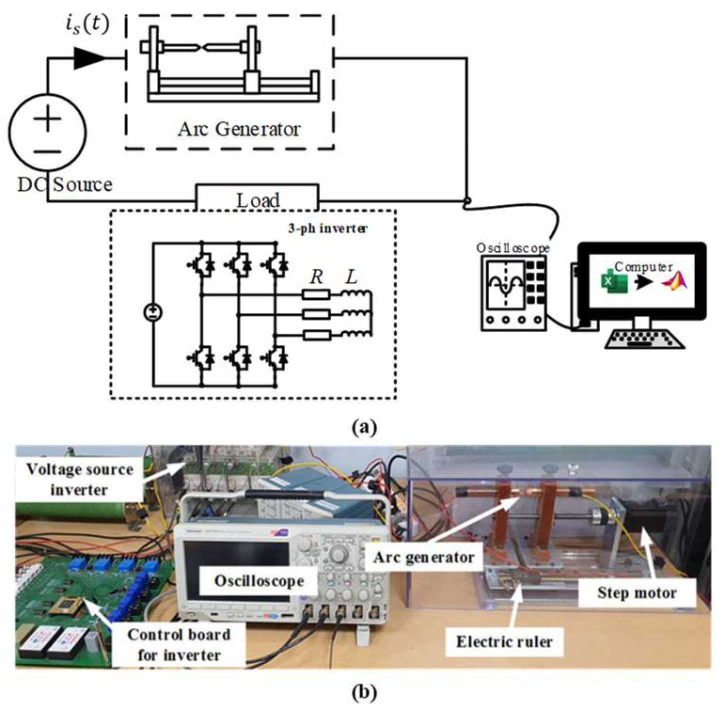
Figure 1 meticulously depicts the intricate dance of data acquisition in our study, emphasizing the rigor and control at the heart of our approach. To ensure scientific robustness, we adhered to the stringent guidelines of UL1699B [25], meticulously crafting the arc-generation circuitry. This carefully calibrated setup utilized the controlled disjointing of arc rods as the precise trigger for arc initiation, immediately followed by the deployment of a high-fidelity oscilloscope, the Tektronix MSO3054 (Tektronix, Beaverton, OR, USA), a high-accuracy oscilloscope known for its reliability and precision. The decision to utilize this particular model was based on its reputation for providing accurate measurements across a wide range of frequencies and signal types. The Tektronix MSO3054 enabled the authors to capture and analyze the data with confidence, ensuring the integrity of our experimental results. Acquired waveforms were then subjected to rigorous analysis via advanced MATLAB routines, extracting the hidden nuances of arcing behavior. The arc generation setup itself was a symphony of essential components: a stable DC power source, a meticulously designed arc generator, and carefully chosen load elements. Figure 1 prominently showcases the N8741A DC power supply from Keysight Technologies (Santa Rosa, CA, USA) delivering precisely controlled DC voltage to the load [26]. An intricate interplay between a high-precision step motor and the customized arc rods ensured their controlled separation, mimicking real-world scenarios with unparalleled precision.
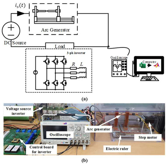
Figure 1.
Arc failure specifications. (a) Setup diagram. (b) Experimental hardware.
For uncompromising data acquisition, authors employed an oscilloscope boasting a stunning 250 kHz sampling frequency, capturing even the most fleeting of electrical nuances. The sampling rate of 250 kHz was selected based on findings from recent investigations into arc faults in DC networks [27,28,29,30]. While a higher sampling rate would yield more data points per unit time, it could also increase processing time and computational burden. Given that a key priority in arc diagnosis is prompt fault identification to swiftly isolate errors from the network, it was imperative to strike a balance between efficiency and execution time. Therefore, the sample rate of 250 kHz was deemed sufficiently high to achieve this equilibrium. Further bolstering our data fidelity, the Tektronix TCP312 (Tektronix, Beaverton, OR, USA) current probe meticulously measured arc currents with surgical accuracy. Our investigation, however, did not merely capture data, it unearthed its meaning through comprehensive exploration. We systematically generated DC arcs under a diverse tapestry of experimental conditions, yielding a rich tapestry of datasets. Each parameter was meticulously chosen, ensuring a comprehensive exploration of potential arc behavior. Our chosen source voltage of 300 V provided a realistic baseline, while current amplitudes spanning 5 to 8 A and switching rates ranging from 5 to 20 kHz pushed the boundaries of arc behavior. To further enrich our understanding, authors explored both resistive (10 Ω) and inductive (10 mH) loads, revealing the nuanced impact of circuit characteristics on arcing phenomena. Figure 1 also unveils the beating heart of our investigation, the three-phase DC–AC converter modules. These inverters, the central load components, played a crucial role in transforming DC signals into their AC counterparts. To ensure precise control, we harnessed the power of space vector modulation (SVPWM) throughout our research. By meticulously manipulating the state of the individual six switching devices within the inverters, authors emulated the sinusoidal waveforms characteristic of the AC network with remarkable fidelity [31]. This fine-grained control allowed us to adjust both frequency and amplitude parameters with exquisite precision, guaranteeing robust and accurate experimental conditions. It is this meticulous orchestration of data acquisition, arc generation, and control circuitry that truly sets our study apart, laying the foundation for a deep and nuanced understanding of DC arc faults.
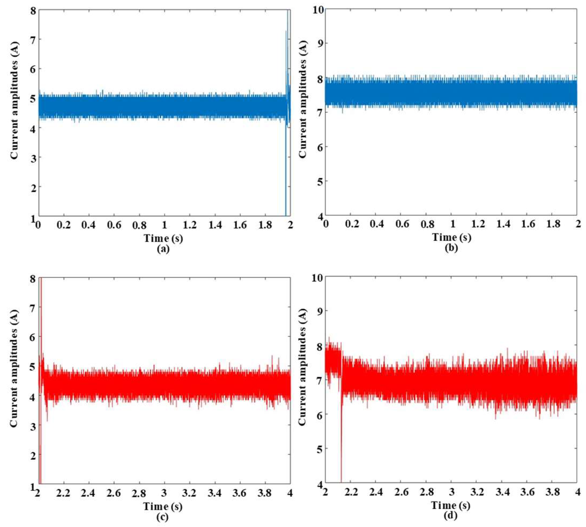
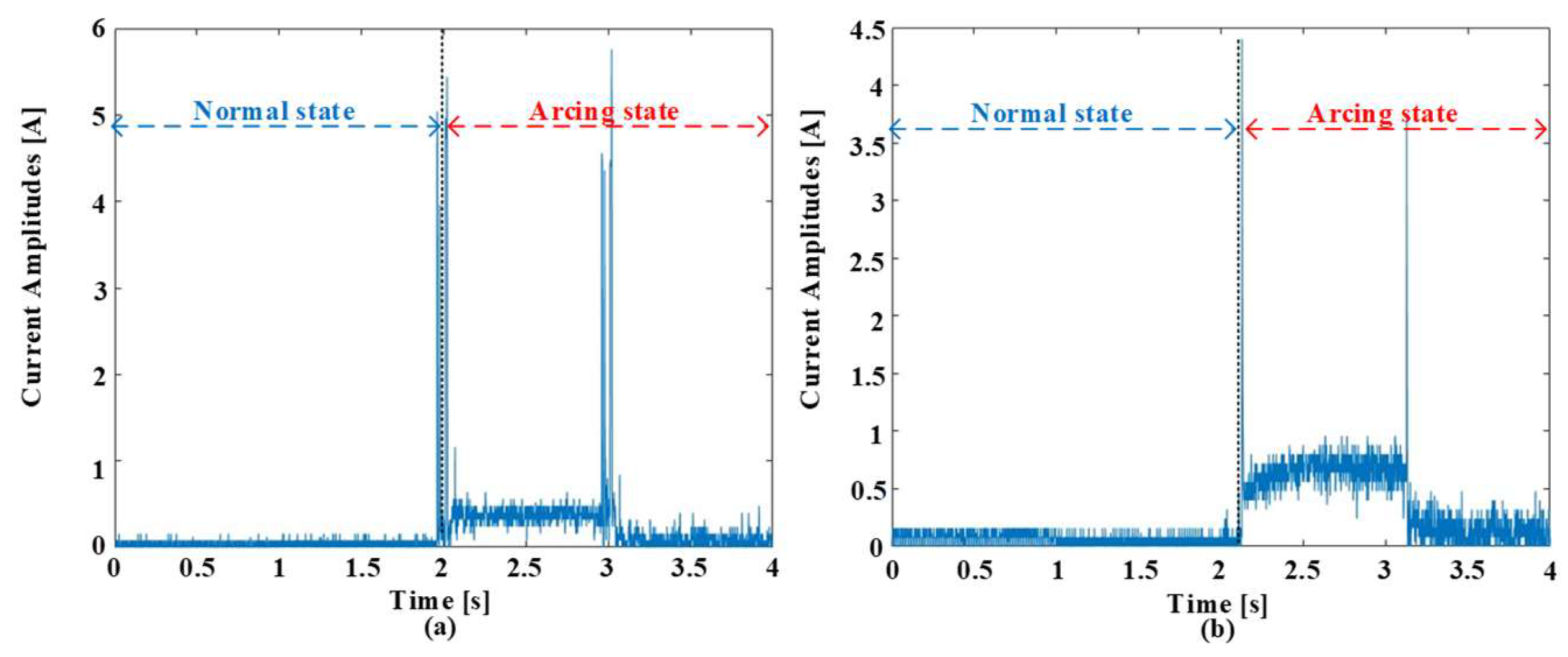
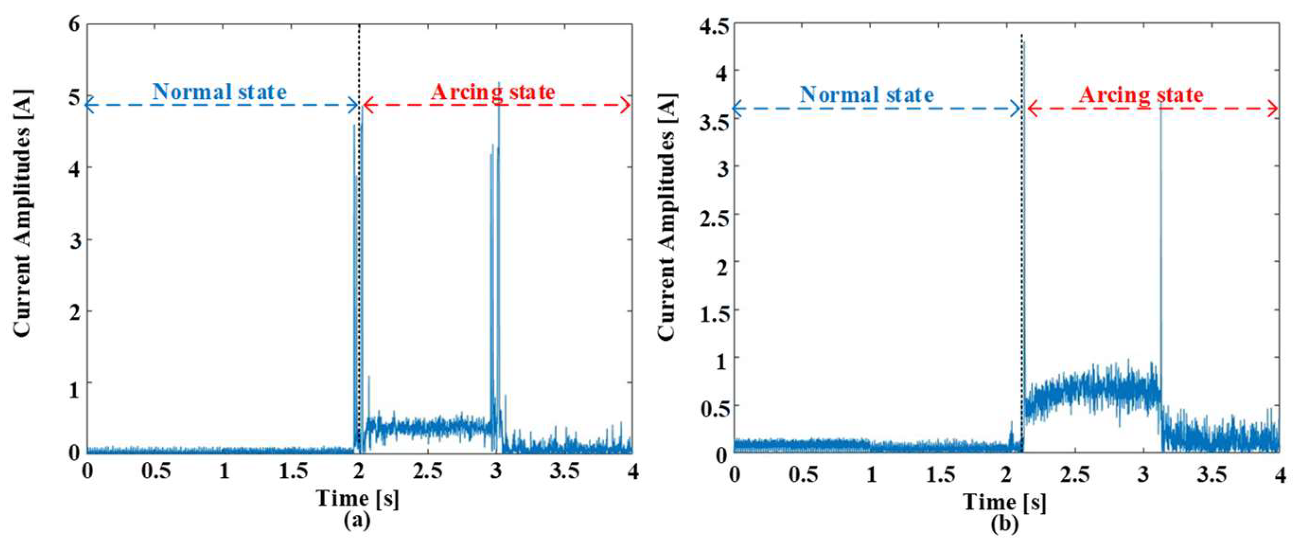
Figure 2 paints a revealing picture of how arc faults dramatically alter the electrical landscape. It showcases waveforms under both normal and arcing conditions at 5 kHz switching frequency and currents of 5 A and 8 A. Although the waveforms follow a similar pattern before the arcing event, the moment an arc forms, the delicate electrical dance erupts into chaos. This chaos manifests in multiple ways. Firstly, harmonic components infiltrate the pure load current, distorting its once smooth rhythm. Imagine ripples spreading across a still pond after a pebble is tossed in. These harmonies, like the ripples, are signatures of the electrical turbulence caused by the arc.
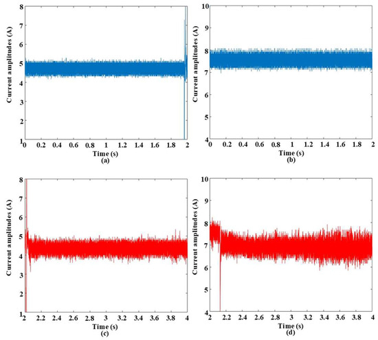
Figure 2.
The current waveforms before and after arc failure at 5 kHz switching frequency. (a) 5 A load current at normal state. (b) 8 A load current at normal state. (c) 5 A load current at arcing state. (d) 8 A load current at arcing state.
Interestingly, the level of distortion seems to be in increased conversation with the switching frequency, suggesting a hidden relationship between these parameters. Secondly, the current amplitude takes a slight dip upon arcing. This subtle but measurable decrease hints at the energy being diverted to sustain the arc itself. Like a siphon stealing water from a pool, the arc siphons off some of the current’s strength. Most striking, however, are the pronounced spikes in amplitude during the initial phase of the arc. These bursts, like tiny electrical explosions, are the telltale signs of the sparky drama unfolding within the circuit. Notably, the intensity of these sparks appears to waltz with the switching frequency, hinting at a deeper connection between frequency and spark magnitude. These dramatic deviations in waveform behavior are more than just visual curiosities; they hold immense promise for the holy grail of arc fault detection. Their unique dance, shaped by the interplay of arcing and switching frequency, offers a potential treasure trove of discriminative features that could unlock the door to accurate and reliable arc fault identification. It is now up to researchers to decipher the language of these electrical hieroglyphs and translate them into effective detection algorithms. The experimental current being lower than the set reference can be attributed to the fact that the impedance of the experimental setup, including the cables, connectors, and components, can introduce voltage drops along the circuit path. These voltage drops can result in a reduction in the effective voltage across the load, leading to a lower current than expected based on the set reference. The distortion in the arc current tends to be higher with higher current amplitudes due to several reasons. At higher current amplitudes, the arc intensity typically increases. This means that the arc becomes more energetic, producing higher temperatures and greater ionization of the surrounding air. As a result, the arc’s behavior becomes more erratic, leading to larger fluctuations and irregularities in the arc current waveform. Additionally, higher current amplitudes lead to increased heating within the arc, resulting in variations in the arc current waveform. Thermal effects can also induce changes in the arc’s size and shape, further contributing to distortion in the arc current waveform.
3. Advanced Learning Techniques and the Differentials of Moving Intervals
3.1. Advanced Learning Techniques
Support Vector Machines (SVMs) are able to uncover the elusive “optimal hyperplane”, a boundary that maximizes the margin between different classes, making them indispensable tools in countless applications. SVMs achieve this by identifying the hyperplane that maximizes this margin, effectively drawing the most distinct and defensible border between classes. They operate with elegance, utilizing a set of weights and biases to define the hyperplane. These weights act like invisible scales, tipping the balance towards one class or another depending on the data point’s features. Biases, on the other hand, function as subtle nudges, fine tuning the position of the hyperplane to ensure the widest possible margin [32]. Imagine data points as individuals in a city, each belonging to a distinct group. KNN throws a data point into this mix and then throws a virtual net around the data point, capturing the k individuals closest to the data point in terms of “distance.” This distance can be measured like footsteps on a city grid (Euclidean distance) or like navigating around buildings (Manhattan distance). It depends on the nature of the data and their characteristics. Once this k-sized neighborhood is established, it becomes the data group, data classification, based on the “votes” of those closest to data point. It is like attending a neighborhood party and declaring your allegiance based on the majority vibe. Choosing the optimal k value, for instance, becomes a strategic balancing act. A small k risks overfitting, basing your identity solely on a handful of noisy neighbors. A large k, on the other hand, can drown out your individuality, making you blend into the city’s overall demographics. Finding the sweet spot for k requires careful consideration of your data and the desired level of granularity [33]. Decision Trees (DTs) are like branching trees, where each path represents a choice and each leaf whispers a prediction. The journey begins at the root, the patriarch of the tree, where the entire dataset gathers. But this root soon splits, driven by a quest for clarity. It analyzes all the features, like a detective interrogating suspects, and identifies the one that best separates the data into distinct groups. This chosen feature becomes the first rule, the first branch in the labyrinth, and like a wise judge dividing disputing parties, the root sends each data point down its designated path based on its feature value. Each branch, in its turn, becomes a new root, a new quest for clarity. The process repeats, with each node splitting based on the most “informative” feature at that level. This dance of splitting continues until the tree reaches its leaf nodes, the quiet corners of the labyrinth where predictions finally bloom. Each leaf represents a distinct category or a specific value, a final destination reached after navigating the intricate web of decisions [34]. One of the most popular ensemble methods is the Random Forest (RF). Think of it as a vast forest of decision trees, each a unique detective with its own set of “if–then” rules. Each tree is trained on a different subset of the data, ensuring no single viewpoint dominates. This diversity is key to the RF’s strength, as it prevents overfitting and allows the forest to capture the intricate patterns hidden within the data. The number of trees, known as a hyperparameter, needs careful tuning. Too few trees limit the forest’s ability to learn complex relationships, while too many lead to computational overload and potentially diminishing returns. Finding the sweet spot, typically within the range of 100 to 1000 trees, is a crucial step in optimizing the RF’s performance. Each tree casts its vote, its prediction based on its own analysis of the data. The RF employs a democratic process. Each vote is weighted based on the tree’s expertise, with more accurate trees having a stronger say in the final decision. This weighted average becomes the collective wisdom of the forest, a prediction refined through the collaboration of diverse perspectives [35]. Naive Bayes (NB) is a statistical sleuth that uses Bayes’ theorem for classification. First, it gathers evidence. It collects information about each possible “culprit” (class) based on prior knowledge and past experience. This initial hunch, the prior probability, gives us a rough idea of who is most likely to be behind the crime (data point). Next, NB examines the individual clues (features) for each suspect. It takes all the evidence, the prior hunch, and the individual clues and combines them using Bayes’ theorem. It assigns the data point to the class with the highest “posterior probability”, the one that emerges as the most likely culprit after considering all the evidence. NB makes an assumption—that the clues (features) are independent gossips, each whispering their suspicions without influencing the others [36].
3.2. Differences of Features between Moving Intervals
This section describes the proposed approach using the differences of features between moving intervals. In this study, the dataset, experimented at a frequency of 250 kHz, is meticulously divided into individual segments, each with an interval of 0.8 ms, to facilitate the subsequent featuring process. Certainly, higher sampling rates could provide more detailed information about the current waveforms and help mitigate issues such as aliasing, noisy data, biasing, and data errors. Adhering to the Nyquist criterion for data sampling is essential for accurately capturing the characteristics of the current signals, especially in dynamic systems prone to rapid changes. In our study, we utilized a sampling frequency of 250 kHz to capture the dynamic nuances of the arc current signals. While this frequency allowed us to effectively capture the essential features of the current waveforms and achieve our research objectives, we acknowledge the potential benefits of higher sampling rates, particularly in scenarios where finer details need to be captured. Within each segment, we diligently calculate the features, such as average, median, RMS, variance, peak-to-peak (p2p), and z-score [37,38]. These features are obtained as follows:
where is the th data element in each data set, and L denotes the number of sampling elements within each sample interval. Then, the differences between features are obtained as follows:
where k is the order of the specified interval and n is the number of the dataset between two intervals. In this study, n is selected to appropriate as a 1250 dataset. Figure 3 paints a fascinating picture of the electrical landscape, revealing the average difference behavior of load current signals under both normal and arcing conditions at two different current amplitudes (5 A and 8 A). Imagine each signal as a river of data points, and the average as a calm pool where these points converge. To find this pool of tranquility, we sum up all the data points in the river and then divide them by their total number, essentially smoothing out the turbulence. Interestingly, the average values reveal a consistent pattern across both normal and arcing states. In the normal state, the river flows serenely, its average level remaining relatively stable, like a placid lake reflecting the sky. In contrast, the arcing state throws the river into turmoil. The average level fluctuates, as if the lake were buffeted by sudden gust of wind, rippling its surface and hinting at the hidden drama unfolding beneath.

Figure 3.
The average differences under different load current amplitudes at 5 kHz switching frequency. (a) Load current at 5 A. (b) Load current at 8 A.
Figure 4 unveils another layer of the electrical drama, this time through the lens of the difference of median. Imagine the data points in our river of information arranged in a line from lowest to highest. The median acts as the silent sentinel, marking the exact point where half the data lies above and half below. It is a robust measure of central tendency, less susceptible to outliers than the average, making it a valuable detective in this electrical mystery. Interestingly, the median paints a similar picture to the average, but with a twist. In the normal state, the median stands resolute, like a lighthouse in calm seas, its value remaining relatively stable over time. This stability whispers of predictability, of a well-behaved electrical system functioning as it should. However, the arcing state throws the median into disarray. It starts to dance erratically, like a ship caught in a storm, reflecting the underlying turbulence caused by the arc. This fluctuating nature of the median in the arcing state holds significant promise as a discriminative feature for classification. It is like a telltale sign, a clue in the electrical fingerprint, that hints at the presence of an arc fault. Unlike the average, which can be skewed by extreme values, the median remains grounded, offering a more robust and reliable indicator of the central tendency.

Figure 4.
The median differences under different load current amplitudes at 5 kHz switching frequency. (a) Load current at 5 A. (b) Load current at 8 A.
Figure 5 unveils yet another hidden dimension of the electrical story, this time through the lens of the Root Mean Square (RMS) difference. Imagine our data points not as a simple line or a single point, but as a bustling crowd of individuals, each representing the signal’s intensity at a specific moment. The RMS acts like a meticulous census taker, calculating the average “loudness” of this crowd, not just by counting heads, but by accounting for the volume of each individual voice. This “loudness” measure, unlike the average or median, is not easily swayed by a few loud outliers. It considers the contributions of all data points, giving a more holistic picture of the crowd’s overall energy. In the normal state, the crowd remains relatively calm, their average volume steady and predictable. It is like a well-behaved orchestra, playing in harmony with no sudden bursts or dramatic crescendos. But when the arc fault strikes, the crowd erupts into chaos. The RMS value spikes, reflecting the sudden surge in signal intensity. This erratic behavior of the RMS in the arcing state provides another valuable clue for classification, a telltale sign that something is amiss in the electrical landscape.
Figure 5.
The RMS differences under different load current amplitudes at 5 kHz switching frequency. (a) Load current at 5 A. (b) Load current at 8 A.
Figure 6 throws a curveball in our electrical detective story, introducing the Peak-to-Peak (p2p) values. Unlike the previous measures, the p2p, which tracks the distance between the highest and lowest points of the signal (think mountain peak to valley floor), does not seem to tell the same tale of clear discrimination between the normal and arcing states. Both the calm symphony of the normal state and the chaotic turbulence of the arcing state appear somewhat muted when viewed through the p2p lens. The peaks and valleys, while present, do not exhibit the dramatic swings we saw in the average, median, or RMS. This suggests that the p2p is not as sensitive to certain aspects of the signal that might be crucial for pinpointing arc faults. The p2p is too focused on the extremes, overlooking the subtle nuances within the signal that betray the presence of an arc. It is like a detective fixated on the most obvious suspects, missing the clever thief hiding in plain sight.

Figure 6.
The p2p differences under different load current amplitudes at 5 kHz switching frequency. (a) Load current at 5 A. (b) Load current at 8 A.
Figure 7 throws a spanner in the works of our electrical detective story. This time, the culprit is the variance, a measure that quantifies how “spread out” a set of values is. Unlike the average, median, or even the dramatic peaks and valleys, the variance seems to struggle to tell the tale of two electrical states. Both the serene drizzle of the normal state and the chaotic downpour of the arcing state appear surprisingly similar through the lens of variance. While some spread is evident in both cases, their values overlap significantly, blurring the lines and making variance an unreliable witness in our quest for fault detection. Variance is too broad of a brush, capturing the overall “noisiness” of the signal but missing the finer details that truly distinguish an arc. Figure 8 throws a wrench in our electrical detective story. This time, the culprit is the z-score, the data’s resident statistician. Unlike the average, median, or even the dramatic peaks and valleys of other features, the z-score seems blind to the contrasting narratives of the normal and arcing states. Both the gentle ebb and flow of the normal state and the turbulent storm surge of the arcing state appear to be mere ripples in z-score’s eyes. While some variation exists, their values overlap significantly, blurring the lines and rendering the z-score an unreliable witness in our fault detection chase. It is like wielding a broad brush, capturing the general “buzz” of the signal but missing the finer details, the subtle whispers that betray the presence of an arc fault.

Figure 7.
The variance differences under different load current amplitudes at 5 kHz switching frequency. (a) Load current at 5 A. (b) Load current at 8 A.
Figure 8.
The z-score under different load current amplitude differences at 5 kHz switching frequency. (a) Load current at 5 A. (b) Load current at 8 A.
The average, median, and RMS values stand tall as reliable witnesses. They whisper clues about the electrical state, with the average portraying a stable melody, the median a steady pulse, and the RMS the overall energy of the electrical storm. These features paint a clear picture, aiding in the discrimination between the serene normalcy and the chaotic arcing states. However, not all features are created equal. The peak-to-peak and variance, like detectives with different specialties, reveal their limitations. The peak-to-peak, focused on the dramatic peaks and valleys, misses the subtle tremors that might betray an arc fault. It is like a detective fixated on a jewel heist, overlooking the clever pickpocket slipping through the crowd. Additionally, the variance, the measure of the overall data spread, becomes overwhelmed by the general “noisiness” of the signal, unable to discern the telltale signature of an arc. Its broad brushstroke blurs the lines between calm and chaos, but this nuanced understanding of different features is precisely what elevates our analysis. It is not about finding a single star witness, but about building a team of diverse perspectives. Each feature, with its strengths and weaknesses, contributes a piece of the puzzle.
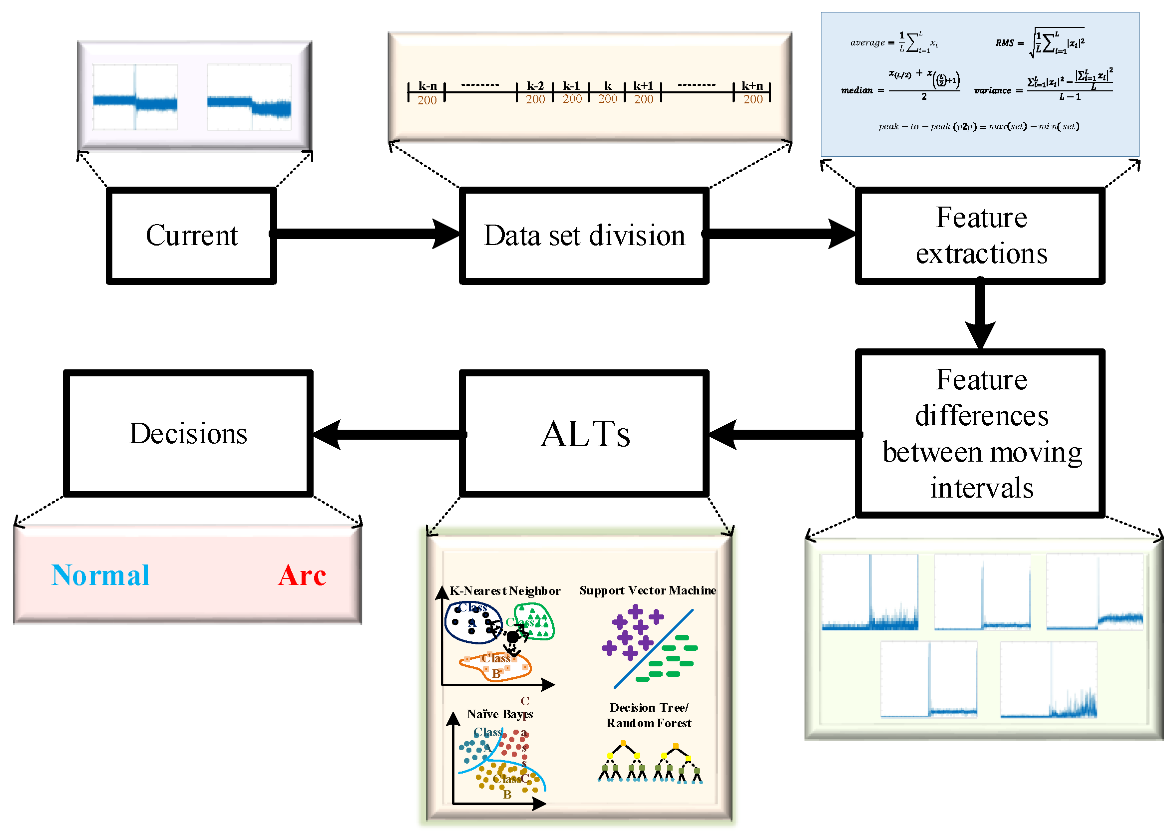
4. Diagnosis of DC Arc-Based Feature Difference of Moving Intervals and Advanced Learning Techniques
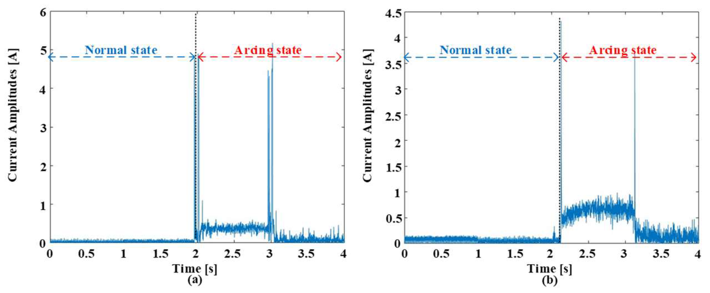
Figure 9 depicts the proposed framework for accurate arc fault diagnosis, employing a data-driven approach. The initial stage involves high-frequency sampling of continuous current data at 250 kHz. This captured data stream is subsequently segmented into subdatasets of 200 data points each, corresponding to a time interval of 0.8 milliseconds. This segmentation facilitates efficient feature extraction and computational tractability. Within each segment, time–domain features are extracted, capturing relevant characteristics of the electrical signal. Crucially, the differences between these features across consecutive segments are calculated, amplifying subtle variations and potentially revealing the presence of arc faults. There are two data ranges of faulted data being tested; the first range is the range of difference between arc and normal states (from 2 s to 3 s). The second range is the difference between arcing states (from 3 s to 4 s). These data ranges will be denoted as R1 (from 2 s to 3 s) and R2 (from 3 s to 4 s). These processed features, enriched with the temporal dynamics of the data, are then fed into advanced learning models. This provides the models with a comprehensive representation of the electrical state, enabling them to learn complex patterns and accurately classify arc faults.
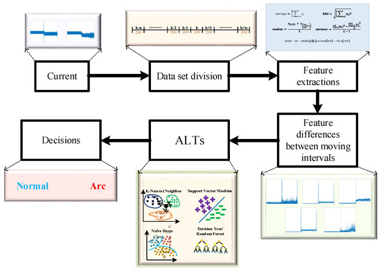
Figure 9.
The proposed diagnosis scheme of DC arc failure using feature differences between moving intervals and ALTs.
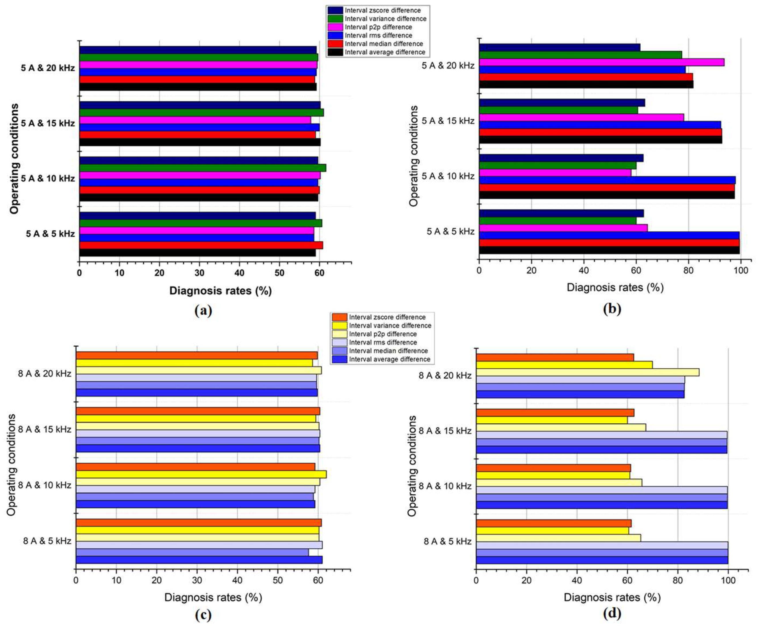
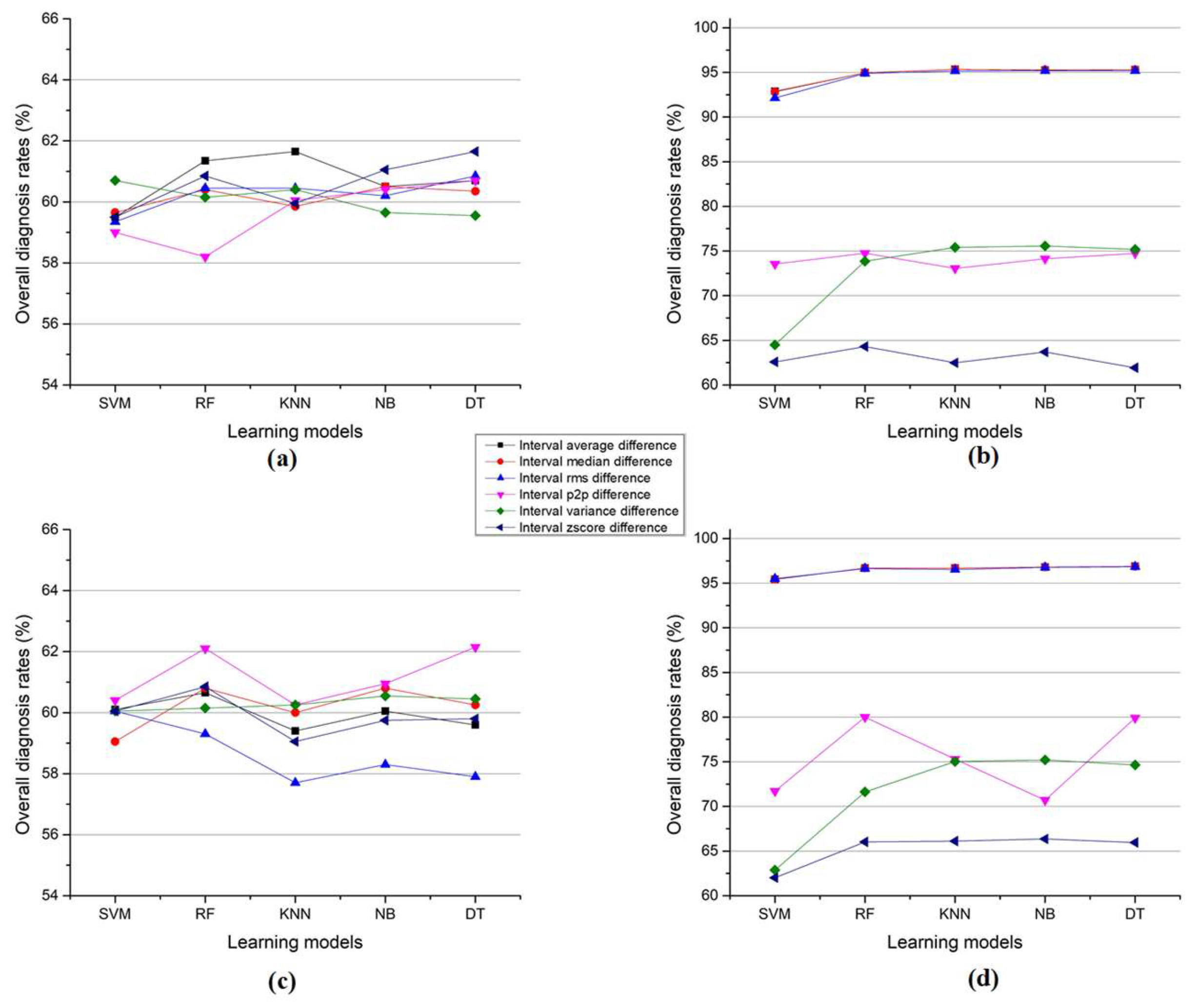
Notably, the framework incorporates both training and testing phases, ensuring the models’ generalizability across diverse operational scenarios and data conditions. Maintaining a balanced data distribution throughout both phases is paramount, with a 1:1 ratio of normal and arcing state data ensuring unbiased training and promoting fair evaluation. This balanced data diet is crucial for the models’ ability to effectively discriminate between normal and arcing conditions with high accuracy. The primary metric employed to assess the performance of the advanced learning models in this context is accuracy. This metric quantifies the models’ ability to correctly identify and classify the electrical state, serving as a fundamental benchmark for performance evaluation. The accuracy metric is calculated as the ratio of correctly classified datasets to the total number of analyzed datasets. Figure 10 illuminates a compelling debate surrounding the efficacy of various features in diagnosing arc faults within a three-phase inverter. It investigates the interplay between current amplitude (5 A and 8 A), switching frequency, and the subsequent accuracy achieved by difference features between moving intervals and the SVM algorithm. The analysis conducted in Section 3 regarding the visibility of feature differences finds validation in Figure 10. The average, median, and RMS values emerge as the frontrunners in terms of accuracy with R1. They operate like seasoned investigators, adept at uncovering subtle clues within the data that betray the presence of an arc fault. However, the plot thickens with the introduction of switching frequency. As it increases, the accuracy of the average, median, and RMS values begins to decline. These features seem overwhelmed by the rapid fluctuations, their focus blurred by the amplified noise. P2P and variance, often less recognized investigative tools, exhibit an inverse relationship, with their accuracy climbing alongside the switching frequency. They shift their focus, honing in on the extreme and rapid changes, finding their own rhythm in the data’s turbulent dance.
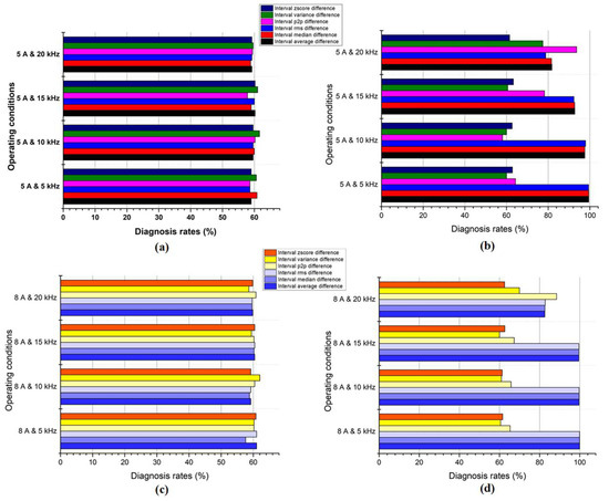
Figure 10.
The diagnosis rates of DC arc failure using featuring differences between moving intervals and SVM. (a) 5 A current R2. (b) 5 A current R1. (c) 8 A current R2. (d) 8 A current R1.
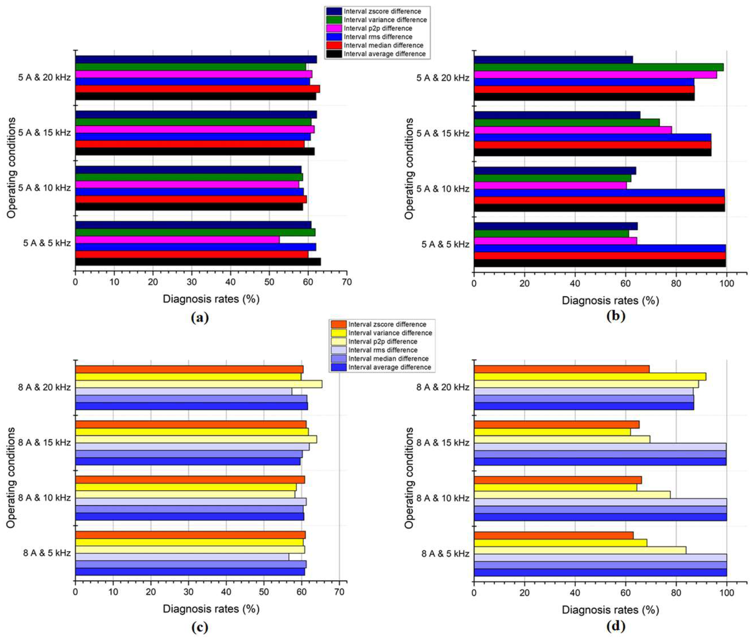
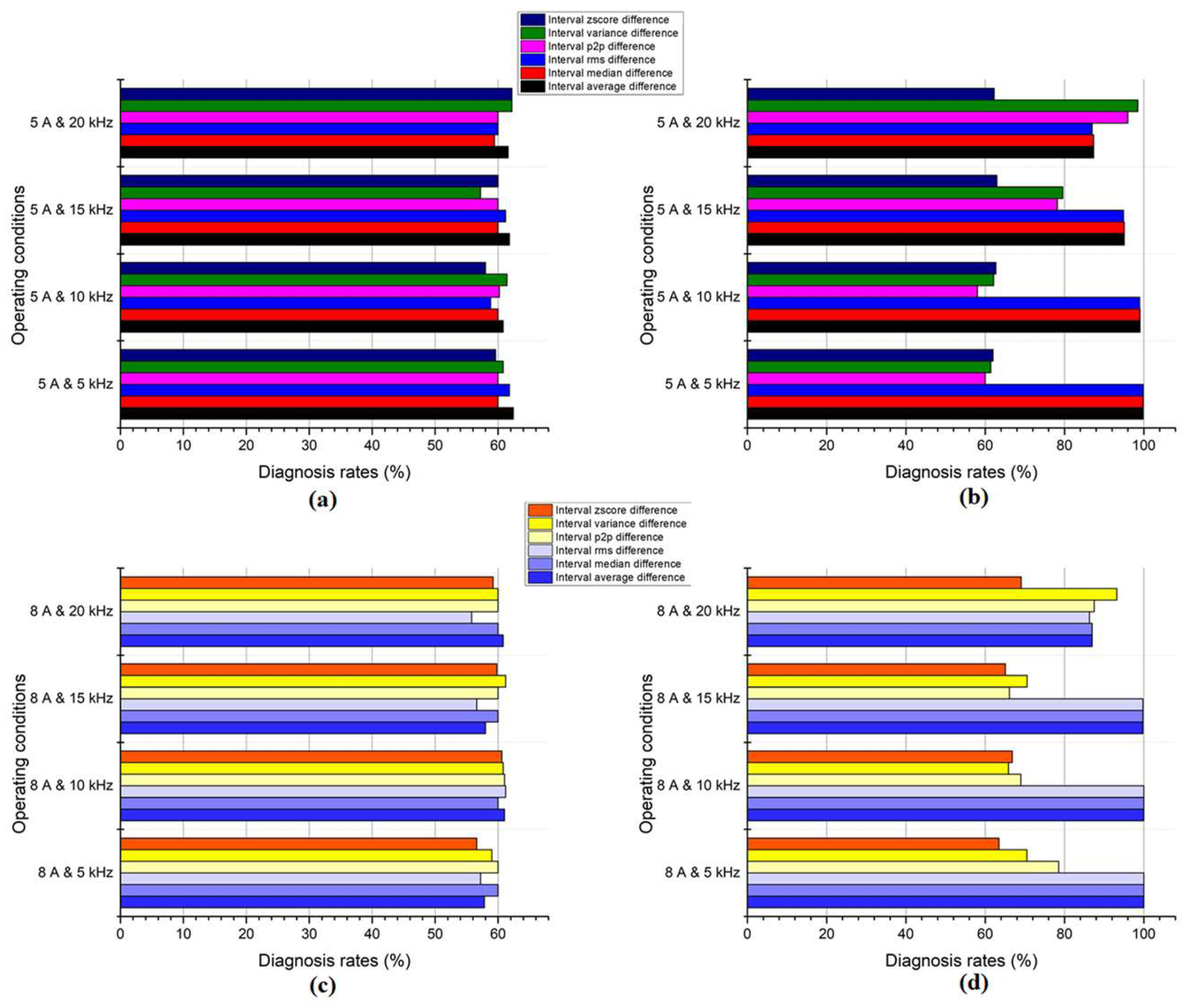
The performance at the 8 A current amplitude presents a particularly intriguing scenario. Here, the accuracy curves for all features converge, with P2P and variance even reaching parity with the average, median, and RMS for R1. Figure 11 explores how different features perform in diagnosing arc faults in a three-phase inverter. It tests them at two current levels (5 and 8 amps) and three switching speeds. For R1, the average, median, and RMS values are the top performers at low speeds, like skilled detectives finding clues in smooth data. But as the switching increases in speed, their accuracy drops, like struggling to keep up with a chaotic crime scene. P2P and variance, often overlooked tools, shine at higher speeds, focusing on sudden changes and data extremes, like detectives chasing a fast-moving suspect. At 8 amps, all features perform similarly, showing the technique’s adaptability. This detective story reveals that different features work best in different situations, and the technique adjusts to ensure accurate diagnoses regardless. Comparing R1 and R1, R1 shows higher accuracy for all features. Figure 12 throws open the case file on arc faults in a three-phase inverter, with the KNN algorithm as our trusty forensic tool. Different features in R1, like the average, median, and RMS, act as seasoned investigators, analyzing data clues to identify the culprit. However, the plot thickens with the rising tide of switching frequency. The rapid electrical fluctuations overwhelm our usual suspects, their focus blurred like detectives in a high-speed chase. P2P and variance, often the overlooked duo, step into the spotlight. They are like hawks circling a carcass, thriving on the data’s extremes and sharp changes. Their unique skills actually benefit from the chaos, and their accuracy soars with faster switching. The 8 A current amplitude introduces another twist. Here, all features find their rhythm, with P2P and variance even matching the established trio.

Figure 11.
The diagnosis rates of DC arc failure using featuring differences between moving intervals and RF. (a) 5 A current R2. (b) 5 A current R1. (c) 8 A current R2. (d) 8 A current R1.

Figure 12.
The diagnosis rates of DC arc failure using featuring differences between moving intervals and KNN. (a) 5 A current R2. (b) 5 A current R1. (c) 8 A current R2. (d) 8 A current R1.
Figure 13 throws shade on the reliability of different tools for spotting arc faults in a three-phase inverter. It tests them at two current levels and three switching speeds, using NB as the detective agency. For R1, the average, median, and RMS are the early stars, like experienced cops good at picking out subtle clues. However, as the switching increases in speed, their accuracy tanks, overwhelmed by the data’s wild swings. P2P and variance, the underdogs, thrive in the chaos, focusing on sudden changes and data extremes, like detectives chasing a fast-moving suspect. For R2, all the features return mediocre performances. At 8 amps, a similar trend as 5 A is observed for both R1 and R2. This shows the outperformance of R1 compared with R2 across various operating conditions. Figure 14 tackles the mystery of arc faults in a three-phase inverter. It is like a detective thriller, where different features, our sleuths, try to solve the case using clues hidden in the data. The criminal’s tactics change with two variables: the electrical flow (5 or 8 amps) and how fast the system switches (frequency). The usual suspects in R1, the average, median, and RMS, are brilliant at low speeds, picking out subtle patterns in the data. However, as the switching becomes faster, the case becomes tricky. They stumble, overwhelmed by the rapid changes, like detectives in a high-speed chase. P2P and variance are often overlooked; they are like hawk-eyed investigators, thriving on the data’s chaos. They zero in on the extremes and swift changes, their accuracy even rising with higher speeds. It is like they’re dancing to the data’s wild rhythm, while the others struggle to keep up. For R2, the accuracies of all features are lower than that of R1 across various current amplitudes and switching frequencies. Figure 15, through its comparative analysis of different features, offers invaluable insights for the future refinement and optimization of DC arc-fault detection. It serves as a guide for developing more effective strategies to apprehend DC arc faults, paving the way for enhanced electrical safety measures and reduced risks of catastrophic events. The results displayed in Figure 10, Figure 11, Figure 12, Figure 13, Figure 14 and Figure 15 were derived from experiments conducted with an AC load configuration encompassing both resistive and inductive elements. The experimental setup was crafted to mirror real-world scenarios, where electrical systems often comprise a diverse array of loads representing a mix of resistive and inductive components. While the primary objective of this study revolves around introducing our methodology and showcasing its effectiveness in detecting arc faults under conditions reflective of real-world load diversity, the authors fully acknowledge the significance of exploring how different load types may influence detection performance. Recognizing the complexity of electrical systems and the potential variations in load characteristics across different applications, the author aims to conduct in-depth analyses to delve into the impact of load composition on the performance of the proposed detection approach. By examining results obtained under varying load conditions, the authors aspire to uncover nuanced insights into the interplay between load types and detection algorithm performance. Ultimately, the aim is to advance the understanding of how different load compositions may impact the efficacy and reliability of arc fault detection algorithms, thus contributing to the development of more robust and adaptive diagnostic techniques for electrical systems. The proposed approach relies on analyzing the difference between moving intervals to detect arc faults in DC circuits. When noise influences the current, it induces fluctuations in both normal and arcing states. However, the fluctuations in the arcing state are typically more pronounced than those in the normal state. As a result, when comparing the difference between the moving intervals, the proposed approach can effectively distinguish between normal operation and arc faults.
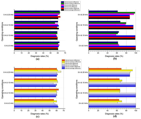
Figure 13.
The diagnosis rates of DC arc failure using featuring differences between moving intervals and NB. (a) 5 A current R2. (b) 5 A current R1. (c) 8 A current R2. (d) 8 A current R1.
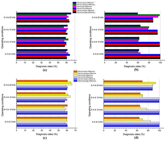
Figure 14.
The diagnosis rates of DC arc failure using feature differences between moving intervals and DT. (a) 5 A current R2. (b) 5 A current R1. (c) 8 A current R2. (d) 8 A current R1.
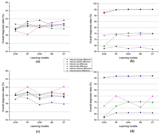
Figure 15.
The diagnosis rates of DC arc failure using feature differences between moving intervals and ALTs. (a) 5 A current R2. (b) 5 A current R1. (c) 8 A current R2. (d) 8 A current R1.
This is because the significant fluctuations observed during arc faults lead to larger differences between consecutive intervals compared to the relatively smaller differences observed during normal operation. By leveraging this characteristic, the proposed approach can accurately detect arc faults by identifying intervals where the difference exceeds a certain threshold. This analysis demonstrates the robustness of the proposed approach in effectively detecting arc faults in DC circuits, even in the presence of noise-induced fluctuations in the current signal.
Indeed, in more complex DC grids, noise on the DC part can arise from various sources, potentially leading to disturbances in the current signal. While the method described in the paper primarily focuses on detecting arc faults induced by the DC/AC inverter, it is important to acknowledge the potential presence of noise in the DC part from other sources. The assumption of relatively low noise in the DC part simplifies the analysis and facilitates the detection of arc faults primarily caused by the DC/AC inverter. However, in real-world scenarios where noise levels may be higher, additional measures may be necessary to account for and mitigate the effects of noise on the accuracy of arc-fault detection. Future research could explore methods to adapt the proposed approach to handle higher levels of noise in the DC part, ensuring robustness and reliability in detecting arc faults in more complex DC grids. In practical applications, it is not uncommon to encounter inverters with switching frequencies exceeding 20 kHz, highlighting the need to address the potential limitations of the proposed method in such scenarios. While the current method primarily focuses on analyzing signals generated by inverters with relatively low switching frequencies compared to the sampling frequency, it is imperative to recognize the impacts of higher switching frequencies on the dynamics of the current signal. Inverter systems with higher switching frequencies may exhibit distinct signal characteristics and behavior, necessitating additional considerations to ensure the effectiveness of the proposed detection method. To address this concern, future research endeavors will delve deeper into the implications of higher switching frequencies on the performance of the proposed method. This exploration will involve analyses to understand how the signal dynamics vary across different switching frequency ranges. Additionally, the authors will investigate potential modifications or adaptations to the existing detection framework to accommodate a broader spectrum of inverter configurations, including those with higher switching frequencies. These modifications may include refining feature extraction techniques, optimizing algorithm parameters, or developing specialized signal processing algorithms tailored to handle the unique challenges posed by high-frequency switching. While the current study focuses on proposing theoretical frameworks and methodologies for arc-fault detection, the authors acknowledge the necessity of experimental validation to assess the practical effectiveness of these approaches in real-world scenarios. However, it is important to emphasize that experimental validation is a critical component that will be executed in future work. Given the complexity and scope of the experimental setup required for rigorous validation, it was deemed prudent to prioritize the development and presentation of robust theoretical frameworks and methodologies in this initial study. These experiments will involve the implementation of the proposed methods in real-world settings, utilizing appropriate hardware setups and data acquisition systems. By conducting experiments under varying conditions and scenarios, the authors aim to evaluate the performance of the approaches in realistic environments and assess their efficacy in accurately detecting arc faults. Indeed, each PWM technique introduces unique variations in the signal characteristics, particularly in response to the occurrence of an arc fault. These variations stem from the specific modulation strategies and switching patterns employed by each PWM technique. For instance, AZPWM, SPWM, and SVPWM each exhibit distinct voltage and current waveforms, harmonics, and switching patterns. When an arc fault occurs, these characteristics may undergo further alterations, such as amplitude fluctuations, frequency shifts, and waveform distortions, depending on the PWM technique implemented. In future work, the authors plan to investigate how these unique variations in signal characteristics, induced by different PWM techniques, can be leveraged in conjunction with our proposed approach for arc detection. By systematically analyzing the response of each PWM technique to arc faults, the authors aim to identify specific features or patterns that are indicative of fault conditions. These features can then be incorporated into our detection algorithm to enhance its robustness and effectiveness across diverse PWM implementations.
5. Conclusions
This pioneering research introduces a novel strategy for addressing the intricate challenge of DC arc-fault detection, leveraging the synergistic capabilities of feature differences between moving intervals and ALTs. Notably, the results highlight the consistent superiority of DT and RF as premier ALTs. These models demonstrate unwavering diagnostic excellence across varying input data scenarios, current amplitudes, and switching frequencies, consistently achieving the highest diagnosis rates. The comparison between different features serves as a focal point for understanding the overarching success of this research. It vividly illustrates the superior performance of ALTs employing diverse input features in the demanding field of DC arc fault detection. Specifically, the average, median, and RMS features emerge as standout performers, outclassing p2p and variance features. This collective success validates the considerable potential of the proposed approach to significantly elevate safety and reliability in electrical systems. Beyond the confines of the laboratory, the real-world implications of this research are substantial, particularly in critical applications like industrial settings and data centers. The groundwork laid by this study contributes to the development of more robust, precise, and dependable arc fault detection systems. These advancements represent promising strides toward enhancing safety and reliability in a diverse range of critical electrical systems, marking a significant step forward in the field.
Author Contributions
Conceptualization, S.K.; methodology, S.K.; software, H.-L.D.; validation, H.-L.D.; formal analysis, S.K.; investigation, H.-L.D.; resources, S.K.; data curation, H.-L.D.; writing—original draft preparation, H.-L.D.; writing—review and editing, S.K. and S.C.; visualization, H.-L.D.; supervision, S.K.; project administration, S.K.; funding acquisition, S.K. All authors have read and agreed to the published version of the manuscript.
Funding
This work was supported by a National Research Foundation of Korea (NRF) grant funded by the Korean government (MSIT) (2020R1A2C1013413).
Data Availability Statement
Data are contained within the article.
Conflicts of Interest
The authors declare no conflicts of interest.
References
- Liang, J.; Jing, T.; Gomis-Bellmunt, O.; Ekanayake, J.; Jenkins, N. Operation and Control of Multiterminal HVDC Transmission for Offshore Wind Farms. IEEE Trans. Power Deliv. 2011, 26, 2596–2604. [Google Scholar] [CrossRef]
- Raza, A.; Dianguo, X.; Xunwen, S.; Weixing, L.; Williams, B.W. A Novel Multiterminal VSC-HVdc Transmission Topology for Offshore Wind Farms. IEEE Trans. Ind. Appl. 2016, 53, 1316–1325. [Google Scholar] [CrossRef]
- Ma, R.; Rong, M.; Yang, F.; Wu, Y.; Sun, H.; Yuan, D.; Wang, H.; Niu, C. Investigation on Arc Behavior During Arc Motion in Air DC Circuit Breaker. IEEE Trans. Plasma Sci. 2013, 41, 2551–2560. [Google Scholar] [CrossRef]
- Sawa, K.; Tsuruoka, M.; Yamashita, S. Fundamental Arc Characteristics at DC Current Interruption of Low Volt-age (<500V), ICEC 2014. In Proceedings of the 27th International Conference on Electrical Contacts, Dresden, Germany, 22–26 June 2014; pp. 1–6. [Google Scholar]
- Kim, Y.-J.; Kim, H. Modeling for Series Arc of DC Circuit Breaker. IEEE Trans. Ind. Appl. 2019, 55, 1202–1207. [Google Scholar] [CrossRef]
- Parise, G.; Parise, L. Unprotected faults of electrical and extension cords in AC and DC systems. IEEE Trans. Ind. Appl. 2014, 50, 4–9. [Google Scholar] [CrossRef]
- Uriarte, F.M.; Gattozzi, A.L.; Herbst, J.D.; Estes, H.B.; Hotz, T.J.; Kwasinski, A.; Hebner, R.E. A DC Arc Model for Series Faults in Low Voltage Microgrids. IEEE Trans. Smart Grid 2012, 3, 2063–2070. [Google Scholar] [CrossRef]
- Gammon, T.; Lee, W.-J.; Zhang, Z.; Johnson, B.C. A review of commonly used DC arc models. IEEE Trans. Ind. Appl. 2015, 51, 1398–1407. [Google Scholar] [CrossRef]
- Khamkar, A.; Patil, D.D. Arc Fault and Flash Signal Analysis of DC Distribution System Sing Artificial Intelligence. In Proceedings of the 2020 International Conference on Renewable Energy Integration into Smart Grids: A Multidisciplinary Approach to Technology Modelling and Simulation (ICREISG), Bhubaneswar, India, 14–15 February 2020; pp. 10–15. [Google Scholar]
- Weerasekara, M.; Vilathgamuwa, M.; Mishra, Y. Modelling of DC Arcs for Photovoltaic System Faults. In Proceedings of the 2016 IEEE 2nd Annual Southern Power Electronics Conference (SPEC), Auckland, New Zealand, 5–8 December 2016; pp. 1–4. [Google Scholar]
- Parise, G.; Martirano, L.; Laurini, M. Simplified Arc-Fault Model: The Reduction Factor of the Arc Current. In Proceedings of the IEEE Industry Applications Society Annual Meeting, Las Vegas, NV, USA, 7–11 October 2012. [Google Scholar]
- Chen, S.; Li, X.; Xiong, J. Series Arc Fault Identification for Photovoltaic System Based on Time-Domain and Time-Frequency-Domain Analysis. IEEE J. Photovolt. 2017, 7, 1105–1114. [Google Scholar] [CrossRef]
- Chae, S.; Park, J.; Oh, S. Series DC Arc Fault Detection Algorithm for DC Microgrids Using Relative Magnitude Comparison. IEEE J. Emerg. Sel. Top. Power Electron. 2016, 4, 1270–1278. [Google Scholar] [CrossRef]
- Zhang, Y.; Wang, L.; Yang, S. Research on Characteristics of DC Arc Fault Based on Wavelet Transform. In Proceedings of the IEEE International Conference on Electrical Systems for Aircraft, Railway, Ship Propulsion and Road Vehicles & International Transportation Electrification Conference (ESARS-ITEC), Nottingham, UK, 7–9 November 2018; pp. 1–6. [Google Scholar]
- Wang, Z.; Balog, R.S. Arc Fault and Flash Signal Analysis in DC Distribution Systems Using Wavelet Transformation. IEEE Trans. Smart Grid 2015, 6, 1955–1963. [Google Scholar] [CrossRef]
- Shimakage, T.; Nishioka, K.; Yamane, H.; Nagura, M.; Kudo, M. Development of Fault Detection System in PV System. In Proceedings of the IEEE 33rd International Telecommunications Energy Conference (INTELEC), Amsterdam, The Netherlands, 8–10 October 2011; pp. 1–5. [Google Scholar]
- Platon, R.; Martel, J.; Woodruff, N.; Chau, T.Y. Online Fault Detection in PV Systems. IEEE Trans. Sustain. Energy 2015, 6, 1200–1207. [Google Scholar] [CrossRef]
- Ducange, P.; Fazzolari, M.; Lazzerini, B.; Marcelloni, F. An Intelligent System for Detecting Faults in Photovoltaic Fields. In Proceedings of the 11th International Conference on Intelligent Systems Design and Applications (ISDA), Cordoba, Spain, 22–24 November 2011; pp. 1341–1346. [Google Scholar]
- Chouder, A.; Silvestre, S. Automatic supervision and fault detection of PV systems based on power losses analysis. Energy Convers. Manag. 2010, 51, 1929–1937. [Google Scholar] [CrossRef]
- Silvestre, S.; Chouder, A.; Karatepe, E. Automatic fault detection in grid connected PV systems. Sol. Energy 2013, 94, 119–127. [Google Scholar] [CrossRef]
- Spataru, S.; Sera, D.; Kerekes, T.; Teodorescu, R. Photovoltaic Array Condition Monitoring based on Online Regression of Performance Model. In Proceedings of the IEEE 39th Photovoltaic Specialists Conference (PVSC), Tampa, FL, USA, 16–21 June 2013; pp. 0815–0820. [Google Scholar]
- Zhang, W.; Xu, P.; Wang, Y.; Li, D.; Liu, B. A DC arc detection method for photovoltaic (PV) systems. Results Eng. 2024, 21, 101807. [Google Scholar] [CrossRef]
- Rong, F.; Huang, C.; Chen, Z.; Liu, H.; Zhang, Y.; Zhang, C. Detection of arc grounding fault based on the features of fault voltage. Electr. Power Syst. Res. 2023, 221, 109459. [Google Scholar] [CrossRef]
- Ji, H.-K.; Wang, G.; Kil, G.-S. Optimal Detection and Identification of DC Series Arc in Power Distribution System on Shipboards. Energies 2020, 13, 5973. [Google Scholar] [CrossRef]
- UL 1699B; Outline of Investigation for Photovoltaic (PV) dc Arc-Fault Circuit Protection, Issue 2. Underwriters Laboratories, Inc.: Northbrook, IL, USA, 2013.
- Kim, J.; Kwak, S. Detection and Identification Technique for Series and Parallel DC Arc Faults. IEEE Access 2022, 10, 60474–60485. [Google Scholar] [CrossRef]
- Dang, H.-L.; Kwak, S.; Choi, S. DC Series Arc Fault Diagnosis Scheme Based on Hybrid Time and Frequency Features Using Artificial Learning Models. Machines 2024, 12, 102. [Google Scholar] [CrossRef]
- Miao, W.; Xu, Q.; Lam, K.H.; Pong, P.W.T.; Poor, H.V. DC Arc-Fault Detection Based on Empirical Mode Decomposition of Arc Signatures and Support Vector Machine. IEEE Sens. J. 2020, 21, 7024–7033. [Google Scholar] [CrossRef]
- Lu, S.; Sirojan, T.; Phung, B.T.; Zhang, D.; Ambikairajah, E. DA-DCGAN: An Effective Methodology for DC Series Arc Fault Diagnosis in Photovoltaic Systems. IEEE Access 2019, 7, 45831–45840. [Google Scholar] [CrossRef]
- Xia, K.; Guo, H.; He, S.; Yu, W.; Xu, J.; Dong, H. Binary classification model based on machine learning algorithm for the DC serial arc detection in electric vehicle battery system. IET Power Electron. 2019, 12, 112–119. [Google Scholar] [CrossRef]
- Dang, H.-L.; Jun, E.-S.; Kwak, S. Reduction of DC Current Ripples by Virtual Space Vector Modulation for Three-Phase AC–DC Matrix Converters. Energies 2019, 12, 4319. [Google Scholar] [CrossRef]
- Boser, B.E.; Guyon, I.M.; Vapnik, V.N. A Training Algorithm for Optimal Margin Classifiers, (COLT’92). In Proceedings of the Fifth Annual Workshop on Computational Learning Theory, New York, NY, USA, 27–29 July 1992; pp. 144–152. [Google Scholar]
- Cover, T.; Hart, P. Nearest neighbor pattern classification. IEEE Trans. Inf. Theory 1967, 13, 21–27. [Google Scholar] [CrossRef]
- Breiman, L.; Friedman, J.; Olshen, R.; Stone, C. Classification and Regression Trees; Wadsworth and Brooks: Belmont, CA, USA, 1984. [Google Scholar]
- Breiman, L. Random forests. Mach. Learn. 2001, 45, 5–32. [Google Scholar] [CrossRef]
- Langley, P.; Iba, W.; Thompson, K. An Analysis of Bayesian Classifiers; NASA Ames Research Center: Moffett Field, CA, USA, 1992; pp. 223–228. [Google Scholar]
- Dang, H.-L.; Kim, J.; Kwak, S.; Choi, S. Series DC Arc Fault Detection Using Machine Learning Algorithms. IEEE Access 2021, 9, 133346. [Google Scholar] [CrossRef]
- Borges, F.A.; Fernandes, R.A.; Silva, I.N.; Silva, C.B.S. Feature Extraction and Power Quality Disturbances Classifcation Using Smart Meters Signals. IEEE Trans. Ind. Inform. 2015, 12, 824–833. [Google Scholar] [CrossRef]


Disclaimer/Publisher’s Note: The statements, opinions and data contained in all publications are solely those of the individual author(s) and contributor(s) and not of MDPI and/or the editor(s). MDPI and/or the editor(s) disclaim responsibility for any injury to people or property resulting from any ideas, methods, instructions or products referred to in the content. |
© 2024 by the authors. Licensee MDPI, Basel, Switzerland. This article is an open access article distributed under the terms and conditions of the Creative Commons Attribution (CC BY) license (https://creativecommons.org/licenses/by/4.0/).