A Hybrid DWA-MPC Framework for Coordinated Path Planning and Collision Avoidance in Articulated Steering Vehicles

Abstract

This paper presents an autonomous collision avoidance method that integrates path planning and control for articulated steering vehicles (ASVs) operating in underground tunnel environments. The confined nature of tunnel spaces, combined with the complex structure of ASVs, increases the risk of collisions due to path-tracking inaccuracies. To address these challenges, we propose a DWA-based obstacle avoidance algorithm specifically tailored for ASVs. The method incorporates a confidence ellipse, derived from the time-varying distribution of tracking errors, into the DWA evaluation function to effectively assess collision risk. Furthermore, the execution accuracy of DWA is improved by integrating a kinematic-based Model Predictive Control. The proposed approach is validated through simulations and field tests, with results demonstrating significant enhancements in collision avoidance and path-tracking accuracy in confined spaces compared to conventional DWA methods.

1. Introduction

Articulated steering vehicles (ASVs) steer by rotating their front and rear bodies relative to each other, offering a smaller turning radius and enhanced maneuverability. These advantages make ASVs widely used for material loading and transportation tasks in underground mines [1]. As mining depths increase, temperature and humidity levels in subterranean environments rise, significantly raising collapse risks and exposing operators to more hazardous conditions. Consequently, developing autonomous driving systems for ASVs has become essential to improve operational safety and efficiency.

Autonomous collision avoidance is a crucial capability for enabling automated driving and ensuring operational safety. Significant advancements have been made in robotic autonomous collision avoidance across various scenarios [2,3,4,5]. Typically, these systems consist of two main components: path planning and path tracking. First, the vehicle generates a feasible local avoidance path based on its surroundings, which is then executed by a tracking controller to enable autonomous navigation and collision avoidance.

Collision-avoidance path planning aims to generate a local path that prevents collisions by following a global path, incorporating real-time environmental data, and considering the vehicle’s kinematic constraints. Key collision-avoidance algorithms include the Dynamic Window Approach (DWA) [6], Artificial Potential Field (APF) [7], and Timed Elastic Band (TEB) [8]. DWA, widely used as the default local planning method in the Robot Operating System (ROS) [9], is one of the most representative methods in local path planning. This approach optimizes obstacle distance, velocity, and heading toward the target by leveraging the robot’s mathematical model. Its effectiveness depends on carefully selected weights for obstacle avoidance, speed, and other parameters in the evaluation function.

Several studies have enhanced the performance of global path planning by integrating A* or Dijkstra algorithms with DWA [10,11,12,13]. In addition, other research has focused on improving the adaptability of DWA in complex environments by incorporating intelligent algorithms like fuzzy control and reinforcement learning [14,15,16,17]. Despite the considerable attention DWA has received, its application is typically limited to differential steering vehicles. This limitation stems from the velocity space used in DWA, which consists of both linear and angular velocities—movements that differential steering vehicles can perform effectively. Although ASVs exhibit rotational behaviors similar to differential steering vehicles when turning, their segmented body structure introduces additional control challenges, making them more complex to handle.

Additionally, a path-tracking controller is essential to achieve closed-loop control for accurate path tracking [18]. For ASVs, geometry-based controllers like the pure pursuit controller [19] are often preferred due to their simplicity and ease of implementation. Beyond these, researchers have developed various advanced controllers, including feedback linearization [20,21], sliding mode control [22], and linear quadratic regulator (LQR) approaches [23], to enhance path-tracking performance. More recently, Model Predictive Control (MPC) has gained significant attention for its superior control capabilities [24]. MPC effectively handles multi-input and multi-constraint vehicle control challenges and enhances system robustness by incorporating predictions of future vehicle states into the optimization process.

Several studies have applied MPC for path tracking of ASVs under diverse operating conditions [25,26,27,28,29]. However, tracking errors are inevitable, and in confined tunnel environments, even minor deviations from the planned path can significantly increase the risk of collisions, potentially resulting in vehicle damage or even casualties. Previous research [30,31,32] has highlighted the critical impact of tracking errors on autonomous vehicle safety by incorporating collision constraints into the MPC optimization process to minimize tracking errors and avoid collisions. Nonetheless, as the number of constraints grows, achieving a globally optimal solution in real-time becomes increasingly challenging, particularly for complex articulated steering vehicles.

In conclusion, achieving autonomous collision avoidance for articulated steering vehicles (ASVs) in narrow underground tunnels remains a significant challenge, mainly due to two factors: (1) limited space, where the confined tunnel environment imposes stringent demands on vehicle maneuverability; and (2) difficulties in maintaining path-tracking accuracy, as the articulated structure of the vehicle introduces control model uncertainties, leading to inevitable tracking errors. To enhance the safety of autonomous collision avoidance for ASVs in underground mines, this paper proposes a collaborative planning and control method. The main contributions of this study are as follows:

(1)

Development of a novel DWA–MPC algorithm: This approach adapts the Dynamic Window Approach (DWA) for ASVs, enhancing path-planning flexibility. By integrating DWA with Model Predictive Control (MPC) based on the vehicle’s kinematic model, the proposed method ensures effective execution of the optimal velocity space generated by DWA.

(2)

Introduction of a collision risk indicator: A new collision risk indicator that accounts for tracking errors is proposed to mitigate collision risks caused by path-tracking inaccuracies. This indicator is incorporated into the DWA evaluation function during the planning process.

(3)

Validation of the proposed algorithm: The collision avoidance performance of the algorithm was verified through co-simulations using MATLAB/SIMULINK 2023 and ADAMS 2020, as well as field tests, demonstrating its effectiveness in enhancing safety.

The structure of this paper is as follows: Section 2 provides an overview of the proposed DWA–MPC framework. Section 3 describes the design of the DWA, including the integration of the collision risk indicator. Section 4 details the MPC design. Experimental results and analysis of the DWA–MPC algorithm are presented in Section 5 and Section 6. Finally, Section 7 offers a brief conclusion and discusses potential directions for future research.

2. Overview of the Proposed DWA–MPC Approach

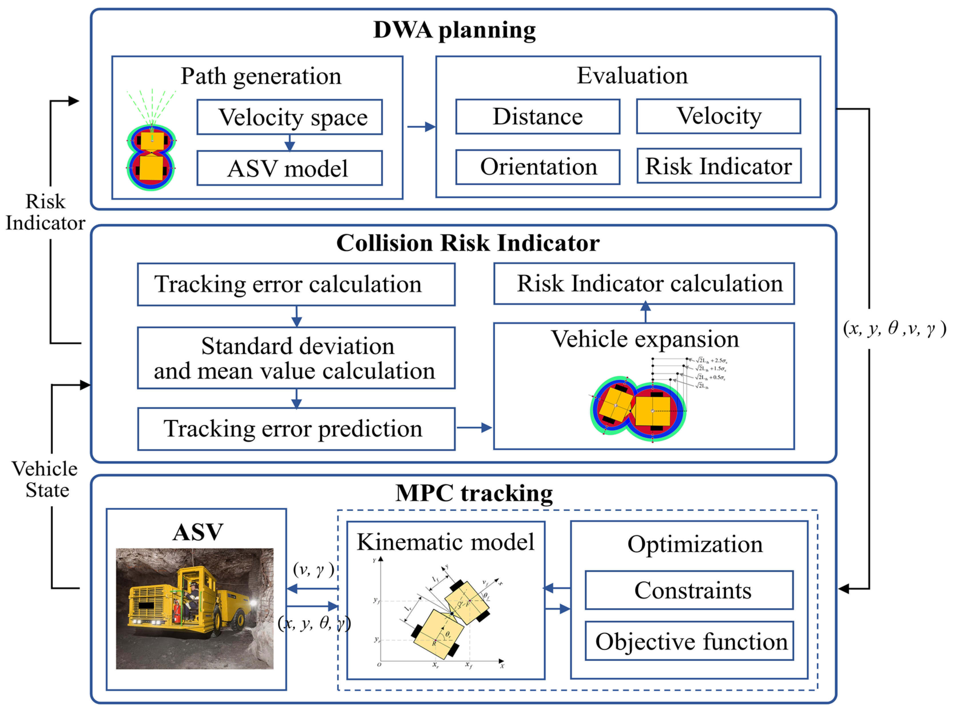
To mitigate the risk of obstacle avoidance failure caused by path tracking errors, we propose a coordinated path planning and control method incorporating DWA and MPC, as illustrated in Figure 1.

First, a Dynamic Window Approach (DWA) algorithm is tailored for ASVs, generating an optimal path based on factors such as obstacle proximity, vehicle orientation toward the target, velocity, and a collision risk indicator. To account for the inherent uncertainties in path tracking, a confidence ellipse is constructed using the distribution of tracking error data over time. The area of this ellipse increases with greater tracking error, reflecting the growing uncertainty. The collision risk is then quantified by measuring the distance between the ellipse’s closest point and the obstacle, and this risk metric is integrated into the DWA evaluation function to reduce collision risks due to tracking uncertainties. Finally, a kinematics-based Model Predictive Control (MPC) is implemented for closed-loop path tracking, ensuring that the ASV accurately follows the planned trajectory, rather than directly applying the control inputs calculated by the DWA to the vehicle.

3. Design of DWA Incorporating Collision Risk Indicator

3.1. DWA Algorithm for ASV

DWA is a common algorithm for local path planning. Firstly, DWA generates the vehicle’s longitudinal velocity and steering angular velocity within defined constraints to form a velocity space. Then, it predicts a motion path in a specified future time by using the vehicle model. These paths are evaluated via an evaluation function so that the path and velocity with the highest score are selected for execution.

3.1.1. Velocity Space

The DWA algorithm needs to account for constraints such as vehicle speed, steering limitations, and braking performance to sample the velocity space and generate combinations of longitudinal velocity and steering angular velocity. The vehicle’s speed and acceleration are constrained according to its specified performance, as illustrated below:

$$\left\{\begin{array}{l}0⩽v(\mathrm{k})⩽v_{\max }\\ v(k)-a_v\Delta t⩽v(k+1)⩽v(k)+a_v\Delta t\\ -{\omega }_{\max }⩽\omega (k)⩽{\omega }_{\max }\\ \omega (k)-a_{\omega }\Delta t⩽{\omega }_1(k+1)⩽{\omega }_1(k)+a_{\omega }\Delta t\end{array}\right.$$

(1)

where $v\left(k\right)$ represents the longitudinal velocity at time step $k$, and $\omega \left(k\right)$ represents the articulated angular velocity at time stepk. The maximum accelerations corresponding to $v\left(k\right)$ and $\omega \left(k\right)$ are $a_v$ and $a_{\omega }$, respectively. $\Delta t$ is the forward simulation time interval.

3.1.2. ASV Model

Based on the generated velocity space, the future states of the vehicle are predicted. To adapt the DWA algorithm for articulated steering vehicles, a kinematic prediction model specific to such vehicles was established. Figure 2 shows its kinematic geometry.

By referring to the kinematic modeling approach described in [29], a kinematic model with the front axle center $(x_f,y_f)$ as the reference point is derived in Equation (2). For simplicity in notation, the subscript f, representing variables $x_f,y_f,{\theta }_f,{\gamma }_f,v_f$ associated with the front body, is omitted to $x,y,\theta ,\gamma ,v$.

$$\left[\begin{array}{c}\dot{x}\\ \dot{y}\\ \dot{\theta }\\ \dot{\gamma }\end{array}\right]=\left[\begin{array}{cc}\cos \theta & 0\\ \sin \theta & 0\\ {\displaystyle \frac{\sin \gamma }{l_f\cos \gamma +l_r}}& {\displaystyle \frac{l_r}{l_f\cos \gamma +l_r}}\\ 0& 1\end{array}\right]\left[\begin{array}{c}v\\ \omega \end{array}\right]$$

(2)

When the vehicle’s initial state is $(x_{k-1},y_{k-1},{\theta }_{k-1},{\gamma }_{k-1})$, and the velocity space is $(v_k,{\omega }_k)$, assuming the vehicle moves at a constant speed over an infinitesimal time interval $\Delta t$, the next state of the vehicle $(x_k,y_k,{\theta }_k,{\gamma }_k)$ can be derived as follows:

$$\left\{\begin{array}{l}{x}_k=x_{k-1}+v_k\cos ({\theta }_{k-1})\Delta t\\ y_k=y_{k-1}+v_k\sin ({\theta }_{k-1})\Delta t\\ {\theta }_k={\theta }_{k-1}+{\displaystyle \frac{(v_k\sin ({\gamma }_{k-1})+l_r\omega )\Delta t}{l_f\cos ({\gamma }_{k-1})+l_r}}\\ {\gamma }_k={\gamma }_{k-1}+{\omega }_k\Delta t\end{array}\right.$$

(3)

where $(x,y)$ represents the center of the front axle; $\theta$ is the heading angle of the front body relative to the global coordinate system; γ is the articulation angle, which denotes the relative angle between the front and rear bodies.

3.1.3. Evaluation Function

To enable effective obstacle avoidance path planning, it is essential to evaluate the generated future states and select an optimal path, utilizing its speed, steering angle, and coordinate information as reference data for the path-tracking controller. The proposed DWA algorithm includes the same evaluation objectives as the traditional DWA algorithm, such as the vehicle’s heading, speed, and distance from the vehicle’s center to obstacles. Additionally, it introduces a collision risk value, which expands the vehicle’s body based on tracking errors to assess the risk. The calculation of this risk value will be elaborated upon in Section 3.2. The evaluate function is shown as:

$$G(\mathrm{v},\omega )=a\cdot heading(\mathrm{v},\omega )+b\cdot dist(\mathrm{v},\omega )+c\cdot vel(\mathrm{v},\omega )-\mathrm{d}\cdot risk$$

(4)

where heading represents the angular difference between the final direction of the predicted path and the target point; dist indicates the distance between the vehicle’s reference center and nearby obstacles; vel is the evaluation function for speed, expressed as the absolute value of the speed; risk accounts for the vehicle’s collision risk value after considering tracking errors. The parameters a, b, c, and d correspond to the weighting coefficients for each respective component. In different application scenarios, achieving optimal results may require adjusting the parameters of various factors. For instance, in scenarios with numerous obstacles or limited space, the weights of b and d should be increased, while those of a and c should be reduced. Conversely, in open driving environments where efficiency is prioritized, the weights of a and c should be increased, while the weights of b and d should be decreased.

3.2. Tracking Error–Informed Collision Risk Indicator

In traditional path planning, vehicles are often assumed to accurately follow the prescribed path. However, due to modeling inaccuracies and external disturbances, the planned path is frequently not executed as intended. For mining articulated vehicles navigating narrow tunnels, neglecting tracking errors in path planning increases the risk of collision. To address this, this section incorporates tracking errors into the planning process by introducing an error-based confidence ellipse.

3.2.1. Tracking Error Calculation

Tracking errors are composed of heading errors $e_h$ and lateral errors $e_d$, as illustrated in Figure 3. The lateral error is a main contributor to vehicle collisions, namely displacement errors. It is defined as the difference in global coordinate position between the nearest point on the reference path and the vehicle’s actual point and is expressed as follows:

$$e_l=(x-x_r)\cos {\theta }_r-(y-y_r)\sin {\theta }_r$$

(5)

where $(x_r,y_r)$ represent the coordinates of the reference point, $(x,y)$ are the coordinates of the actual position, and ${\theta }_r$ is the heading angle of the reference point.

3.2.2. Tracking Error Prediction

The tracking error at the current moment may not fully represent the tracking error at future moments. Given the tracking errors are unlikely to change significantly over a short period, the range of future tracking errors can be inferred from the distribution of past tracking errors. Assuming the tracking error data follows a normal distribution, it can be characterized by its mean and standard deviation to describe the probability density, as illustrated in Figure 4. For instance, the probability that the error falls within $\left(-0.5\sigma ,0.5\sigma \right)$ is 38%, and the probability that the error data falls within $\left(-1.5\sigma ,1.5\sigma \right)$ is 87%. To consider the effects of tracking errors during path planning, the mean and standard deviation of tracking error data from time $k-n$ to $k$ are calculated to estimate the probability density of future tracking errors. The equations for calculating the mean and standard deviation are as follows:

$$\left\{\begin{array}{l}\overline{x}={\displaystyle \sum _{i=1}^n\frac{e_i}{n}}\\ \sigma =\sqrt{{\displaystyle \frac{1}{n}}{\displaystyle \sum _{i=1}^n{(e_i-\overline{x})}^2}}\end{array}\right.$$

(6)

where $n$ is the sample size and $e_i$ is the tracking error for the i-th sample.

3.2.3. Confidence Ellipse-Based Vehicle Expansion

We expand the vehicle’s body based on the distribution density of tracking error data at specific step sizes. This expansion enables the calculation of distances to obstacles, ensuring adequate space is maintained between the vehicle and potential obstacles. The confidence ellipse method is employed to represent the distribution of two-dimensional data, where the lengths of the semi-major and semi-minor axes correspond to the standard deviations along different dimensions [33].

Drawing from this method, we treat the body of the articulated steering vehicle as an inscribed rectangle within an ellipse. By combining the vehicle’s dimensions with the standard deviations of the tracking errors, we generate expansion areas at different confidence levels for collision risk detection. The semi-major axis $l_{long}$ and semi-minor axis $l_{short}$ of the vehicle’s confidence ellipse are, respectively, represented as follows:

$$\begin{array}{l}{l}_{long}=\alpha \cdot l_{f1}+\left(\overline{x}+\beta \cdot \sigma \right)\\ l_{short}=\alpha \cdot l_{f2}+\left(\overline{x}+\beta \cdot \sigma \right)\end{array}$$

(7)

where $l_{f1}$ and $l_{f2}$ represent the length and width of the vehicle; $\alpha$ is the coefficient of the inscribed rectangle; $\beta$ is the coefficient of the standard deviation, which can be adjusted to obtain different probability densities.

Figure 5 shows the generated collision risk areas, in which ➀, ➁, and ➂ are the confidence regions for β = 0.5, 1.5, and 2.5, respectively. Based on the probability density distribution, it is estimated that the vehicle has probabilities of (38%)², (50%)², and (90%)² of being located in the different regions at the next moment. By adjusting the standard deviation coefficient $\beta$, the size of the confidence region can be dynamically tailored to suit planning tasks with different objectives. Additionally, reducing the extent of the confidence region helps to lower the computational complexity of the algorithm.

3.2.4. Risk Indicator Calculation

To quantitatively describe collision risk in greater detail, we divide the collision risk detection area into three non-overlapping regions. Based on the distribution probabilities within each region, the probabilities of the vehicle’s future position falling within these areas are 0.144, 0.613, and 0.233, respectively. The proximity of an obstacle to the vehicle directly correlates with an increased collision risk. Consequently, we inversely adjust the vehicle’s collision risk indicator based on the probability density. The Risk indicator can be expressed as follows:

$$Risk=\left\{\begin{array}{cc}0& P\notin ①,②,③\\ 0.233& P\in ①\\ 0.233+0.613& P\in ②\\ 0.233+0.613+0.144& P\in ③\end{array}\right.$$

(8)

where P is the region in which the nearest obstacle is located.

4. Design of MPC for Tracking DWA Planned Path

Differential steering vehicles can achieve the linear and angular velocities required by the DWA algorithm by controlling the speed differential between the wheels on each side. However, for ASVs, the fixed relative position between the body and wheels, combined with the split-body structure, leads to more complex dynamic responses. Using open-loop control, where the DWA algorithm solely drives the vehicle forward and steers, often results in significant tracking errors. To address this, we propose a lower-level MPC algorithm tailored for the DWA algorithm when applied to ASVs. By incorporating the same kinematic model used in the DWA, we establish a cohesive link between the planning and control layers.

Let the state variable be defined as $\chi =[x,y,\theta ,\gamma {]}^T$ and the control variable as $u=[v,\omega {]}^T$. The kinematic model presented in Equation (2) directly aligns with the path state and velocity space of the DWA planning algorithm described in Section 3. The kinematic model is expressed as follows:

$$\dot{\chi }=f(\chi ,u)$$

(9)

To enhance the computational efficiency of the predictive model, a first-order Taylor expansion is performed on Equation (9) at the desired path point $({\chi }_d,u_d)$, linearizing the kinematic model. The model is then discretized by the forward Euler method, resulting in a linearized discrete kinematic model:

$$\overline{\chi }\left(k+1\right)=A_k\overline{\chi }\left(k\right)+B_k\overline{u}\left(k\right)$$

(10)

where $A_k=\left[\begin{array}{cccc}1& 0& -v_d\sin {\theta }_{d}T& 0\\ 0& 1& v_d\cos {\theta }_{d}T& 0\\ 0& 0& 1& {\displaystyle \frac{v_d(l_f+l_r\cos {\gamma }_d)+{\omega }_d{l}_f{l}_r\sin {\gamma }_d}{{\left(l_f\cos {\gamma }_d+l_r\right)}^2}}T\\ 0& 0& 0& 1\end{array}\right]$, $B_k=\left[\begin{array}{cc}\cos {\theta }_{d}T& 0\\ \sin {\theta }_{d}T& 0\\ {\displaystyle \frac{\sin {\gamma }_r}{l_f\cos {\gamma }_r+l_r}}T& {\displaystyle \frac{l_r}{l_f\cos {\gamma }_r+l_r}}T\\ 0& T\end{array}\right]$, $\overline{u}(k)=\left[\begin{array}{c}v(k)-v_d(k)\\ \omega (k)-{\omega }_d(k)\end{array}\right]$, $\overline{\chi }(k)=\left[\begin{array}{c}x(k)-x_d(k)\\ y(k)-y_d(k)\\ \theta (k)-{\theta }_d(k)\\ \gamma (k)-{\gamma }_d(k)\end{array}\right]$.

To predict the state variables at future time steps, a new state variable is defined as $\xi (k)=\left[\begin{array}{c}\overline{\chi }\left(k\right)\\ \overline{u}(k-1)\end{array}\right]$. Using the linearized discrete kinematic model (10), the following equation is derived as follows:

$$\xi (k+1)=\overline{A}\xi \left(k\right)+\overline{B}\Delta u\left(k\right)$$

(11)

$$\eta \left(k\right)=\overline{C}\xi \left(k\right)$$

(12)

where $\overline{A}=\left[\begin{array}{cc}{A}_k& B_k\\ 0_{m\times n}& I_m\end{array}\right]$, $\overline{B}=\left[\begin{array}{c}{B}_k\\ I_m\end{array}\right]$, $\overline{C}=\left[\begin{array}{cc}{I}_n& 0\end{array}\right]$, $\Delta u=\overline{u}(k)-\overline{u}(k-1)$, n and m denote the dimensions of the state variable and the control variable, respectively.

Let N_p be the prediction horizon and N_c be the control horizon, we can derive the predictive equation for the state variables at future time steps, expressed as follows:

$$Y=\Psi \xi (k)+\Theta \Delta U$$

(13)

where $\Psi =\left[\begin{array}{c}\overline{C}\overline{A}\\ \overline{C}{\overline{A}}^2\\ \dots \\ \overline{C}{\overline{A}}^{N_c}\\ \dots \\ \overline{C}{\overline{A}}^{N_p}\end{array}\right]$, $\Theta =\left[\begin{array}{ccccc}\overline{C}\overline{B}& 0& 0& \cdots & 0\\ \overline{C}\overline{A}\overline{B}& \overline{C}\overline{B}& 0& \cdots & 0\\ \cdots & \cdots & \cdots & \ddots & \cdots \\ \overline{C}{\overline{A}}^{N_c-1}\overline{B}& \overline{C}{\overline{A}}^{N_c-2}\overline{B}& \overline{C}{\overline{A}}^{N_c-3}\overline{B}& \cdots & \overline{C}{\overline{A}}^0\overline{B}\\ \cdots & \cdots & \cdots & \ddots & \cdots \\ \overline{C}{\overline{A}}^{N_p-1}\overline{B}& \overline{C}{\overline{A}}^{N_p-2}\overline{B}& \overline{C}{\overline{A}}^{N_p-3}\overline{B}& \cdots & \overline{C}{\overline{A}}^{N_p-N_c}\overline{B}\end{array}\right]$, $\Delta U=\left[\begin{array}{c}\Delta \overline{u}(k)\\ \Delta \overline{u}(k+1)\\ \Delta \overline{u}(k+2)\\ \begin{array}{c}\dots \\ \Delta \overline{u}(k+N_c-1)\end{array}\end{array}\right]$, $Y=\left[\begin{array}{c}\eta (k+1)\\ \eta (k+2)\\ \eta (k+3)\\ \dots \\ \eta (k+N_p)\end{array}\right]$.

Finally, based on the predictive equation, we construct a cost function shown in Equation (14). By solving it, we obtain $\Delta U$ that minimizes the error between the state values and the desired values within the prediction horizon N_p, while also minimizing the variation in the input:

$$\begin{gathered} \min J(\xi (k),u(k-1),\Delta U))={\displaystyle {\sum }_{i=1}^{N_p}{‖\eta (k+i)-{\eta }_d(k+i)‖}_Q^2}+{{\displaystyle {\sum }_{i=1}^{N_c}‖\Delta U(k+i)‖}}_R^2+{\tau }^2 \\ \begin{array}{ll}\mathbf{s.t.}& \Delta U_{\min }\le \Delta U(k)\le \Delta U_{\max }\\ & U_{\min }\le U(k-1)+\Delta U(k)\le U_{\max }\\ & Y_{\min }-\tau \le \psi \xi (k)+\Theta \Delta U(k)\le Y_{\max }+\tau \end{array} \end{gathered}$$

(14)

where the relaxation factor τ can prevent the controller from encountering infeasible solutions; ${\eta }_d$ is provided by the optimal path generated by the DWA; $\left[\Delta U_{\min },\Delta U_{\max }\right]$ is the constraint range for the control input increments; $\left[U_{\min },U_{\max }\right]$ is the constraint range for the control input.

5. Simulation Experiments

To assess the performance of the proposed algorithm, a path-tracking experiment was initially conducted to evaluate the stability of the control system. Confidence ellipses were constructed based on the tracking error, providing further validation of the method. Additionally, the algorithm’s obstacle avoidance capabilities were tested in both narrow alley turns and obstacle avoidance scenarios to comprehensively evaluate its effectiveness. A co-simulation was conducted using MATLAB/SIMULINK 2023 and ADAMS 2020 dynamic analysis software to verify the proposed algorithm. An ADAMS model of ASV acted as the control object, providing real-time kinematic responses of the vehicle, as shown in Figure 6. The simulation was executed on a high-performance computer equipped with an Intel Core i7-13700 CPU and 32 GB RAM.

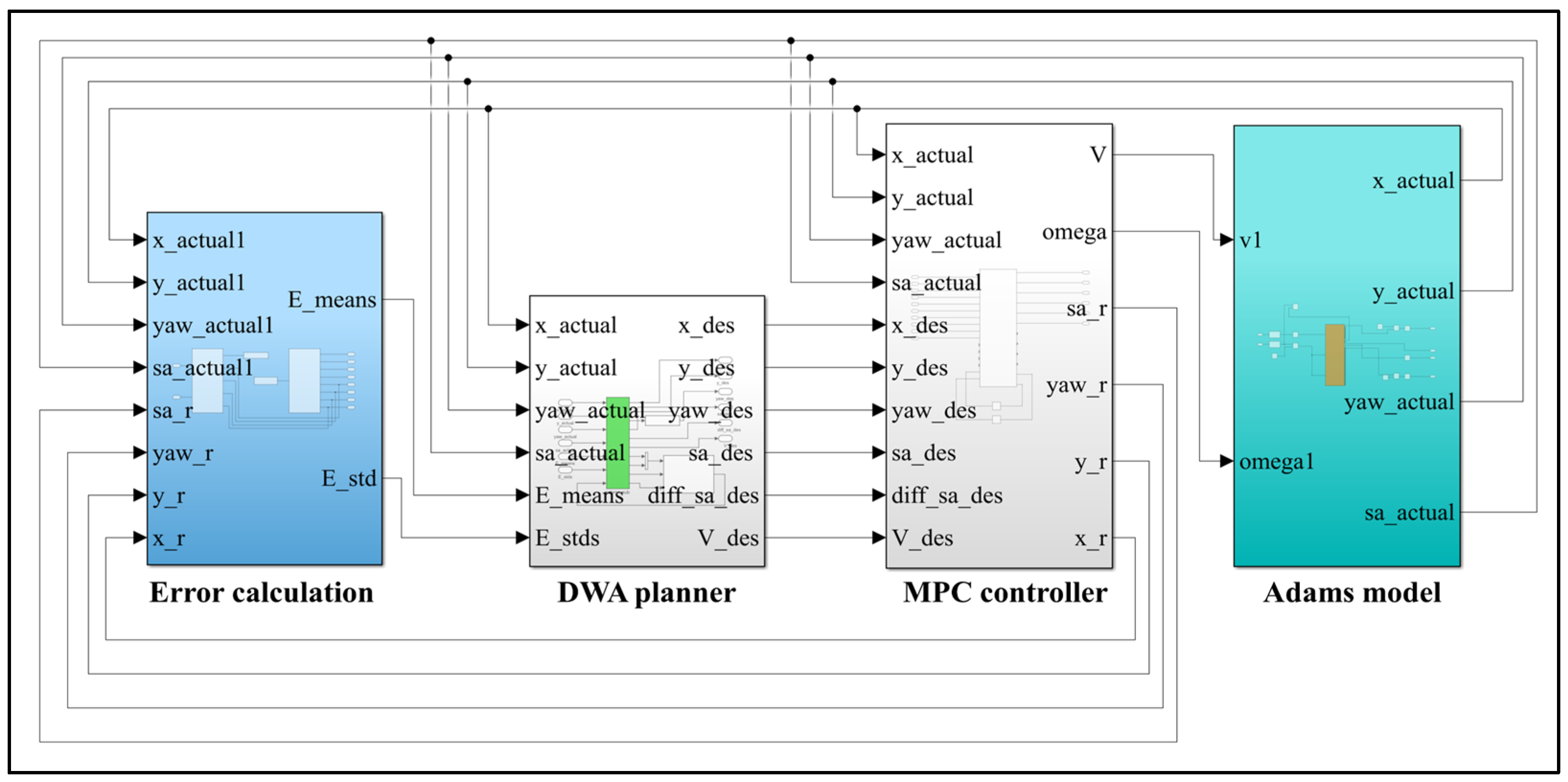
The simulation architecture is depicted in Figure 7. Within the MATLAB/SIMULINK environment, modules were developed to handle error calculation, the DWA planner with risk indicators, and MPC algorithms. The DWA planner module incorporated virtual obstacle scenarios to dynamically compute the distances between obstacles and the vehicle. Simultaneously, an ASV model was created in ADAMS, with constraints and parameters referenced from [34]. The geometric parameters of the model are listed in

Table 1. The model parameters.

Parameter and Unit	Description	Value
$l_a$ (m)	Total length of the vehicle	1.18
$l_{f1}$ (m)	Front body length	0.46
$l_{f2}$ (m)	Front body width	0.6
$l_{r1}$ (m)	Rear body length	0.62
$l_{r2}$ (m)	Rear body width	0.55

. The SIMULINK and ADAMS environments were synchronized with a sampling interval of 0.01 s.

5.1. Path Tracking Experiment

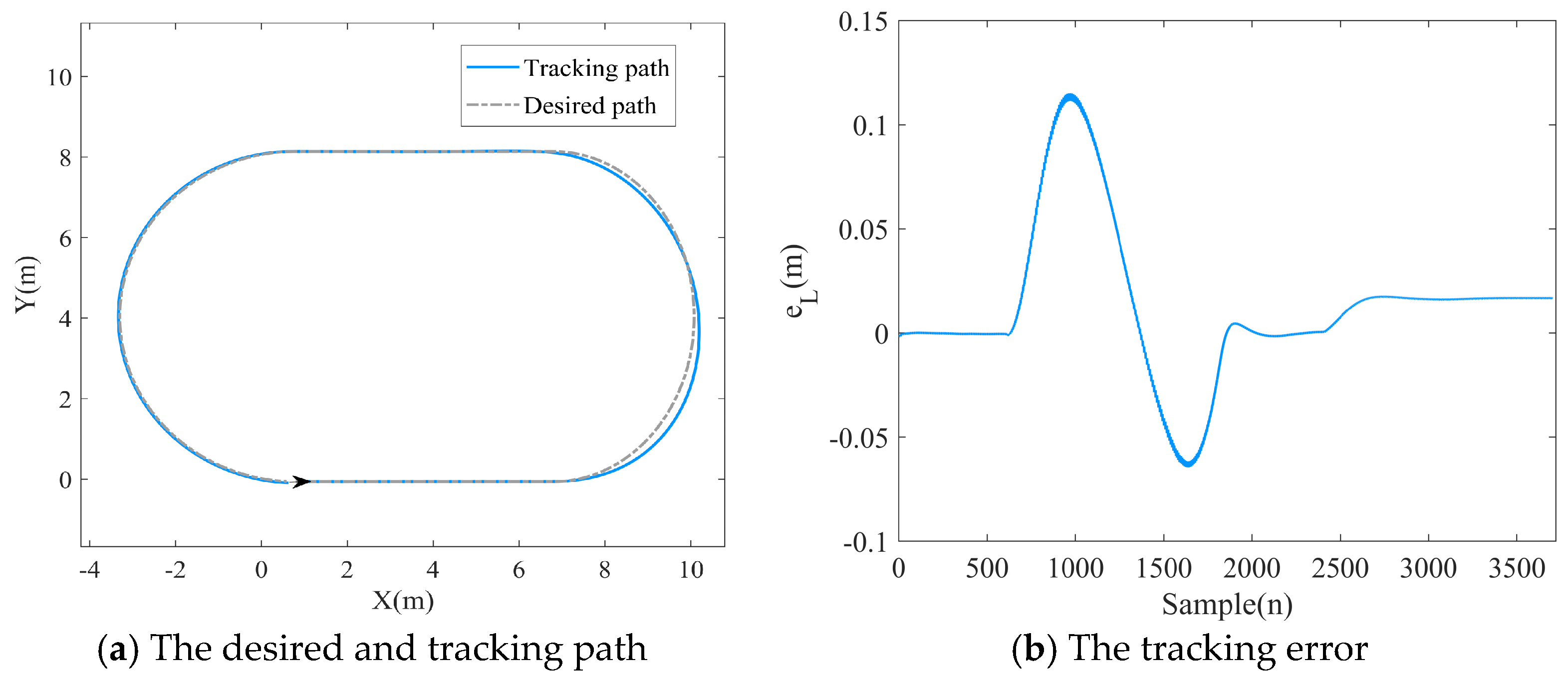
A path comprising both straight and turning segments was designed to assess the stability of the control algorithm. The tracking path, represented by the gray dashed line in Figure 8, consists of two semi-circles with a radius of 2 m and two straight sections, each 8 m long. To simulate uncertainty during tracking, a steering angle pulse disturbance of 0.1 radians amplitude and 0.1 s duration was introduced during the first turn. The controller parameters are provided in

Table 2. The controller parameters.

Parameters	Np	Nc	Q	R	$\mathit{\tau }$	${\mathit{v}}_{\mathbf{max}}$	${\mathit{\omega }}_{\mathbf{max}}$
Value	50	20	10	5	0.01	2 m/s	0.25 rad/s

.

The tracking results shown as the blue solid line in Figure 8, together with the lateral error data in Figure 9, indicate that the proposed MPC path tracking algorithm can accurately follow the desired path. Under external disturbances, the system remained stable, achieving a root mean square (RMS) lateral error of 0.02 and a maximum error of 0.11. Using the vehicle expansion method described in Section 3.2, we computed the tracking error data over 500 timesteps (5 s prior tracking moment) and constructed the expanded region based on the error confidence ellipses. This expanded region was subsequently visualized, as illustrated in Figure 9.

To improve clarity, we visualized selected sample points distributed along the entire path. The results show that when the tracking error is small, the risk region is the same size as the vehicle body, with the deep blue and green confidence ellipses almost overlapping the red region. This occurs because the area of the elliptical risk region is determined by the standard deviation of the tracking error. When the error is small, the data are more concentrated over a specific time period, resulting in lower dispersion and a smaller standard deviation, which causes the three ellipses to nearly overlap.

As the error increased, the data dispersion within a specific period also rose, resulting in a larger standard deviation and varying areas for the three ellipses. For instance, during the first turn, external disturbances caused the tracking error to increase, leading to an expansion of the risk region. This demonstrates that the proposed method for constructing collision risk effectively captures the uncertainty introduced by tracking errors, thereby offering valuable guidance for path planning.

5.2. Collision Avoidance Experiment

To further evaluate the obstacle avoidance performance of the proposed DWACR-MPC algorithm, we conducted tests in both narrow alley turning and obstacle avoidance scenarios. We compared the results with other algorithms: DWA and TEB that directly apply the optimal velocity space for vehicle control and the DWA–MPC algorithm, which does not account for collision risks. Both DWA and MPC utilized the same kinematic model and velocity constraints. Moreover, the forward simulation time in DWA was set to 50 steps, aligning with the N_p in MPC.

5.2.1. Narrow Alley Turning Scenario

Figure 10 depicts a narrow alley turning scenario with a lane width of 1 m by black bold lines. The vehicle needs to navigate this narrow road and successfully reaches the target point at (10, 10). A front-wheel steering vehicle can complete the turn in this space if its length is less than a specific multiple of the lane width. In comparison, the ASV has a smaller turning radius than the front-wheel steering vehicle. With a length of 1.18 m, the test vehicle model demonstrates that the designed scenario meets the necessary turning requirements.

Figure 11 illustrates the results of controlling the ADAMS model using the DWA and TEB algorithms. The gray dashed line represents the global planning path. The light blue solid line and the yellow vehicle body denote the trajectory generated by the DWA algorithm, while the dark red dotted line and the red vehicle body represent the trajectory produced by the TEB algorithm. While the vehicle successfully follows the planned path during straight-line motion, both algorithms encounter difficulties during turns, leading to significant tracking errors. These errors cause the vehicle to collide with the inner corner of the curve, resulting in task failure. Analysis reveals that although ASVs share some similarities with differential steering vehicles, such as maintaining a fixed position between the wheels and the body, the articulated steering vehicle’s segmented body structure results in a more complex kinematic model. When using only DWA or TEB, the system behaves as an open-loop control, making precise tracking challenging. As a result, there is a high probability of the vehicle deviating from the planned path, increasing the risk of task failure.

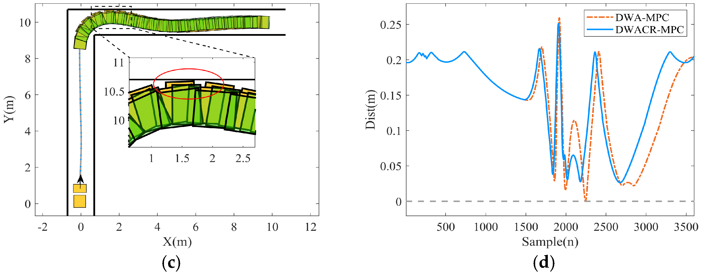
Figure 12 illustrate the collision avoidance results obtained using the DWA–MPC algorithm. Figure 12a presents the driving results when the vehicle collision risk indicator is not considered. The enlarged view shows the vehicle’s front body contacting the edge of the corridor, while the collision risk visualization indicates that the vehicle occupies the highest risk region, highlighted in red. The root mean square (RMS) tracking errors are 0.03 m for both algorithms, regardless of whether the collision risk indicator is considered, as shown in Figure 12b.

Compared to using DWA alone, integrating the DWA planning algorithm with the MPC algorithm improves the vehicle’s execution accuracy. In Figure 12c, the green and yellow vehicles represent the tracking control results with and without consideration of the collision risk indicator, respectively. In the high-risk turning area, the green vehicle demonstrates a larger safety margin compared to the yellow vehicle. Figure 12d further illustrates the variation in the minimum distance between the vehicle and obstacles. When the collision risk indicator is considered, the minimum distance from obstacles increases by 0.03 m. In contrast, when the collision risk indicator is ignored, the minimum distance is reduced to 0 m, leading to contact with the corridor during turns.

5.2.2. Obstacle Avoidance Scenario

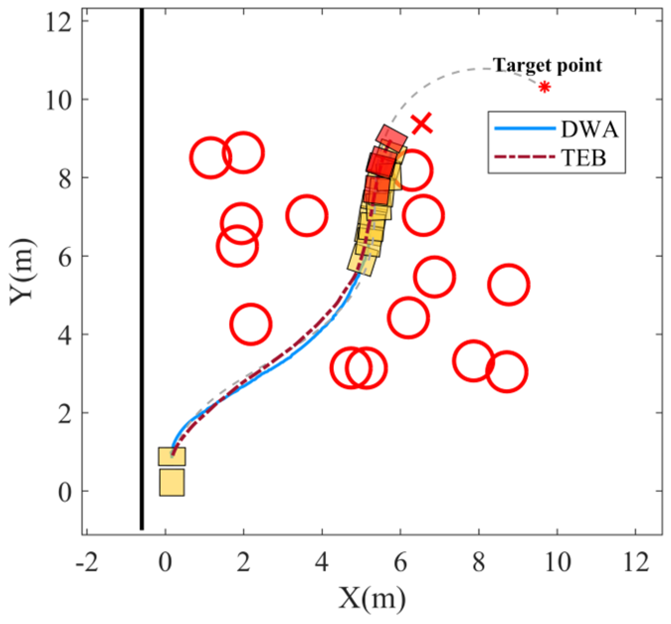
Next, we evaluated the performance of the proposed algorithm in a more open obstacle avoidance scenario, with the vehicle’s target point set at coordinates (10, 10). Figure 13 illustrates this setup, featuring 15 circular obstacles, each with a radius of 0.5 m, randomly distributed throughout the environment. In Figure 13, the obstacles are represented by bold solid red lines. To ensure the vehicle navigates through the obstacles rather than bypassing them, a barrier was placed 0.2 m from the vehicle’s perimeter.

The results of using only the DWA or TEB algorithms are presented in Figure 14. Similarly to the outcomes observed in alley turning scenario relying solely on the DWA or TEB algorithm for planning and control proves insufficient for safely reaching the target point, as the vehicle collides with obstacles in narrow spaces. Figure 15 shows the result of the DWA–MPC algorithm. Figure 15a presents the driving path of DWA–MPC without the vehicle collision risk indicator. The vehicle body is expanded and visualized based on the method in Section 3.2.3. The planned path displays continuously varying curvature, which leads to increased tracking error. In comparison to the narrow alley turning scenario, the vehicle’s risk region expands larger. The lateral tracking error curve in Figure 15b indicates that the DWACR–MPC algorithm, which accounts for collision risk areas, effectively reduces the tracking error, decreasing the RMS value of the lateral error from 0.08 to 0.05.

In Figure 15c, the green and yellow vehicle trajectories represent the results of motion with and without consideration of the collision risk indicator, respectively. The DWA–MPC algorithm, which did not incorporate collision risk assessment, resulted in minor vehicle scraping during tight turns in constrained spaces. As shown in Figure 15d, this led to instances where the distance to the obstacle became negative. In contrast, the DWACR–MPC algorithm successfully navigated through the obstacles, maintaining a minimum clearance of 0.25 m and reaching the target point, thereby demonstrating its superior performance.

6. Field Experiment

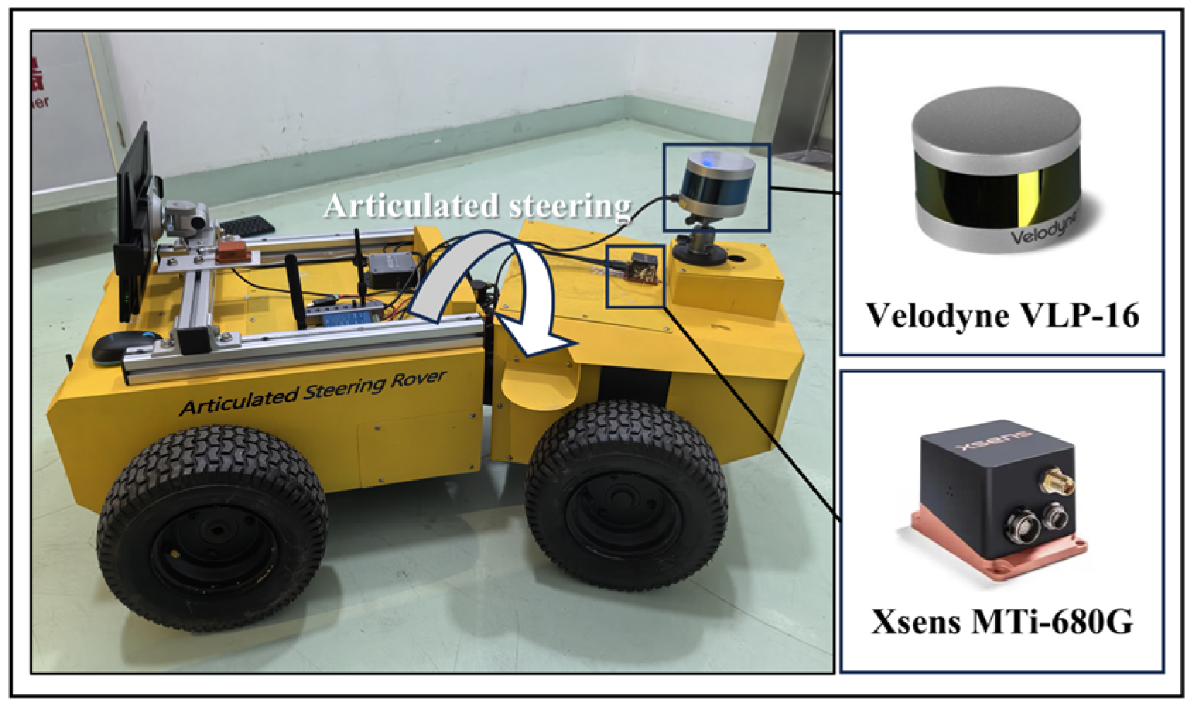
To evaluate the performance of the proposed algorithm, we conducted field tests in an indoor corridor using a 1:4 scale articulated vehicle prototype. The prototype shown in Figure 16 features a steering mechanism identical to that of a mining articulated vehicle, with dimensions of 1250 mm in length, 710 mm in width, and 410 mm in height. The test platform integrates a 16-line LiDAR and a high-precision inertial navigation system, employing the Faster-LIO algorithm [35] for indoor positioning and environmental perception. An industrial control computer, equipped with an Intel I7-6700 processor and 32 GB of memory, serves as the computing platform, with the algorithm running on the ROS1 framework.

Figure 17 displays the point cloud image and photos of the indoor corridor scene. This scene resembles the environment of underground mine car driving, with limited space relative to the vehicle size. The corridor width is 2100 mm, narrowing to just 1600 mm at its narrowest point. The test prototype must safely navigate from the starting point to the endpoint autonomously. We conducted performance tests on the DWA–MPC and DWACR–MPC algorithms, with the results presented in Figure 18.

To clearly illustrate the algorithm results, we proportionally simplified the corridor environment in Figure 18. The simplified corridor, represented by the bold black line, was constructed based on point cloud coordinates. Figure 18a presents the driving path of DWACR–MPC and the visualized result of the vehicle expansion. During the turn, the tracking error increases, causing the vehicle body’s expanded area to grow. This observation aligns the field test results with the simulation outcomes. In Figure 18b, the yellow vehicle body and the gray dotted line represent the motion path of DWA–MPC, while the green vehicle body and the blue solid line represent the motion path of DWACR–MPC. Combining the obstacle-vehicle distance in Figure 18c, it is evident that DWA–MPC collides when turning near the end. However, DWACR–MPC introduces a vehicle body expansion method based on tracking errors, preventing collisions and successfully completing the driving task. This experimental result demonstrates the algorithm’s effectiveness.

7. Conclusions

In this paper, we present a coordinated planning and control algorithm, called DWA–MPC, tailored for autonomous collision-avoidance navigation in underground mining articulated steering vehicles. First, a DWA algorithm customized for ASVs was developed, incorporating a collision risk indicator to select optimal paths. This DWA algorithm is then integrated with a kinematics-based MPC to improve tracking accuracy. Collision risk is assessed by analyzing tracking error distribution over a specified period and is factored into the DWA evaluation function. Experimental results demonstrate that the proposed method significantly enhances both collision-avoidance capabilities and path-tracking precision. By modifying the vehicle model within the framework, this method can also be applied to vehicles with different steering mechanisms, thereby enhancing collision avoidance safety during operation.

To ensure the algorithm’s effective operation, it is essential to store the tracking error over a defined period and compute the minimum distance between the expansion vehicle and obstacles. This process imposes significant demands on the device’s computational capacity. In future research, efforts will focus on further optimizing the algorithm’s complexity by adaptively adjusting it to compute and store error frequencies. Additionally, as DWA parameter selection affects planning outcomes, we plan to incorporate reinforcement learning and other intelligent algorithms for adaptive parameter tuning, improving the adaptability and robustness of the planning algorithm.

References

1. Marshall, J.; Barfoot, T.; Larsson, J. Autonomous underground tramming for center-articulated vehicles. J. Field Robot. 2008, 25, 400–421. [Google Scholar] [CrossRef]
2. Ji, J.; Khajepour, A.; Melek, W.; Huang, Y. Path planning and tracking for vehicle collision avoidance based on model predictive control with multi-constraints. IEEE Trans. Veh. Technol. 2016, 66, 952–964. [Google Scholar] [CrossRef]
3. Wang, N.; Xu, H. Dynamics-constrained global-local hybrid path planning of an autonomous surface vehicle. IEEE Trans. Veh. Technol. 2020, 69, 6928–6942. [Google Scholar] [CrossRef]
4. Song, K.; Sun, Y. Coordinating multiple mobile robots for obstacle avoidance using cloud computing. Asian J. Control 2021, 23, 1225–1236. [Google Scholar] [CrossRef]
5. Luo, D.; Huang, X.; Huang, Y.; Miao, M.; Gao, X. Optimal Trajectory Planning for Wheeled Robots (OTPWR): A Globally and Dynamically Optimal Trajectory Planning Method for Wheeled Mobile Robots. Machines 2024, 12, 668. [Google Scholar] [CrossRef]
6. Fox, D.; Burgard, W.; Thrun, S. The dynamic window approach to collision avoidance. IEEE Robot. Autom. Mag. 1997, 4, 23–33. [Google Scholar] [CrossRef]
7. Lee, M.; Park, M. Artificial potential field-based path planning for mobile robots using a virtual obstacle concept. In Proceedings of the IEEE/ASME International Conference on Advanced Intelligent Mechatronics, Kobe, Japan, 20–24 July 2003. [Google Scholar]
8. Wu, J.; Ma, X.; Peng, T.; Wang, H. An improved timed elastic band (TEB) algorithm of autonomous ground vehicle (AGV) in complex environment. Sensors 2021, 21, 8312. [Google Scholar] [CrossRef]
9. Dobrevski, M.; Skočaj, D. Adaptive dynamic window approach for local navigation. In Proceedings of the 2020 IEEE/RSJ International Conference on Intelligent Robots and Systems, Las Vegas, NV, USA, 25–29 October 2020. [Google Scholar]
10. Liu, H.; Zhang, Y. An improved A-star algorithm for indoor cleaning robots. IEEE Access 2022, 10, 99498–99515. [Google Scholar] [CrossRef]
11. Guo, H.; Li, Y.; Wang, H.; Wang, C.; Zhang, J.; Wang, T.; Rong, L.; Wang, H.; Wang, Z.; Huo, Y.; et al. Path planning of greenhouse electric crawler tractor based on the improved A* and DWA algorithms. Comput. Electron Agr. 2024, 227, 109596. [Google Scholar] [CrossRef]
12. Liu, L.; Lin, J.; Yao, J.; He, D.; Zheng, J.; Huang, J.; Shi, P. Path planning for smart car based on Dijkstra algorithm and dynamic window approach. Wirel. Commun. Mob. Comput. 2021, 2021, 8881684. [Google Scholar] [CrossRef]
13. Wu, B.; Chi, X.; Zhao, C.; Zhang, W.; Lu, Y.; Jiang, D. Dynamic path planning for forklift AGV based on smoothing A* and improved DWA hybrid algorithm. Sensors 2022, 22, 7079. [Google Scholar] [CrossRef] [PubMed]
14. Dobrevski, M.; Skočaj, D. Dynamic Adaptive Dynamic Window Approach. IEEE Trans. Robot. 2024, 40, 3068–3081. [Google Scholar] [CrossRef]
15. Lin, Z.; Yue, M.; Chen, G.; Sun, J. Path planning of mobile robot with PSO-based APF and fuzzy-based DWA subject to moving obstacles. Trans. Inst. Meas. Control 2022, 44, 121–132. [Google Scholar] [CrossRef]
16. Chang, L.; Shan, L.; Jiang, C.; Dai, Y. Reinforcement based mobile robot path planning with improved dynamic window approach in unknown environment. Auton. Robot. 2021, 45, 51–76. [Google Scholar] [CrossRef]
17. Patel, U.; Kumar, N.; Sathyamoorthy, A.; Manocha, D. DWA-RL: Dynamically feasible deep reinforcement learning policy for robot navigation among mobile obstacles. In Proceedings of the IEEE International Conference on Robotics and Automation (ICRA), Xi’an, China, 30 May–5 June 2021. [Google Scholar]
18. Stano, P.; Montanaro, U.; Tavernini, D.; Tufo, M.; Fiengo, G.; Novella, L.; Sorniotti, A. Model predictive path tracking control for automated road vehicles: A review. Annu. Rev. Control 2023, 55, 194–236. [Google Scholar] [CrossRef]
19. Fue, K.; Porter, W.; Barnes, E.; Li, C.; Rains, G. Autonomous navigation of a center-articulated and hydrostatic transmission rover using a modified pure pursuit algorithm in a cotton field. Sensors 2020, 20, 4412. [Google Scholar] [CrossRef]
20. Zhao, X.; Yang, J.; Zhang, W.; Zeng, J. Feedback linearization control for path tracking of articulated dump truck. Telkomnika 2015, 13, 922–929. [Google Scholar] [CrossRef]
21. Dekker, L.G.; Marshall, J.A.; Larsson, J. Experiments in feedback linearized iterative learning-based path following for center-articulated industrial vehicles. J. Field Robot. 2019, 36, 955–972. [Google Scholar]
22. Nayl, T.; Nikolakopoulos, G.; Gustafsson, T.; Kominiak, D.; Nyberg, R. Design, and experimental evaluation of a novel sliding mode controller for an articulated vehicle. J. Robot. Auton. Syst. 2018, 103, 213–221. [Google Scholar] [CrossRef]
23. Yu, H.; Zhao, C.; Li, S.; Wang, Z.; Zhang, Y. Pre-work for the birth of driver-less scraper (LHD) in the underground mine: The path tracking control based on an LQR controller and algorithms comparison. Sensors 2021, 21, 7839. [Google Scholar] [CrossRef]
24. Ding, Y.; Wang, L.; Li, Y.; Li, D. Model predictive control and its application in agriculture: A review. Comput. Electron. Agric. 2018, 151, 104–117. [Google Scholar] [CrossRef]
25. Nayl, T.; Nikolakopoulos, G.; Gustafsson, T. Effect of kinematic parameters on MPC based on-line motion planning for an articulated vehicle. Robot. Auton. Syst. 2015, 70, 16–24. [Google Scholar] [CrossRef]
26. Bai, G.; Liu, L.; Meng, Y.; Luo, W.; Gu, Q.; Ma, B. Path tracking of mining vehicles based on nonlinear model predictive control. Appl. Sci. 2019, 9, 1372. [Google Scholar] [CrossRef]
27. Shi, J.; Sun, D.; Qin, D.; Hu, M.; Kan, Y.; Ma, K.; Chen, R. Planning the trajectory of an autonomous wheel loader and tracking its trajectory via adaptive model predictive control. J. Robot. Auton. Syst. 2020, 131, 103570. [Google Scholar] [CrossRef]
28. Zhou, B.; Su, X.; Yu, H.; Guo, W.; Zhang, Q. Research on Path Tracking of Articulated Steering Tractor Based on Modified Model Predictive Control. Agriculture 2023, 13, 871. [Google Scholar] [CrossRef]
29. Chen, X.; Yang, C.; Cheng, J.; Hu, H.; Shao, G.; Gao, Y.; Zhu, Q. A Novel Iterative Learning-Model Predictive Control Algorithm for Accurate Path Tracking of Articulated Steering Vehicles. IEEE Robot. Autom. Lett. 2024, 9, 7373–7380. [Google Scholar] [CrossRef]
30. Jian, Z.; Yan, Z.; Lei, X.; Lu, Z.; Lan, B.; Wang, X.; Liang, B. Dynamic control barrier function-based model predictive control to safety-critical obstacle-avoidance of mobile robot. In Proceedings of the IEEE International Conference on Robotics and Automation (ICRA), London, UK, 30 May–1 June 2023. [Google Scholar]
31. Ammour, M.; Orjuela, R.; Basset, M. An MPC combined decision making and trajectory planning for autonomous vehicle collision avoidance. IEEE Trans. Intell. Transp. Syst. 2022, 23, 24805–24817. [Google Scholar] [CrossRef]
32. Lindemann, L.; Dimarogonas, D.V. Barrier function based collaborative control of multiple robots under signal temporal logic tasks. IEEE Trans. Control. Netw. Syst. 2020, 7, 1916–1928. [Google Scholar] [CrossRef]
33. Wang, B.; Shi, W.; Miao, Z. Confidence analysis of standard deviational ellipse and its extension into higher dimensional Euclidean space. PLoS ONE 2015, 10, e0118537. [Google Scholar] [CrossRef]
34. Yang, C.; Zhu, Q.; Liu, Q.; Chen, X. An unscented Kalman filter based velocity estimation method for articulated steering vehicles using a novel dynamic model. Proc. Inst. Mech. Eng. Part K J. Multibody Dyn. 2023, 237, 389–405. [Google Scholar] [CrossRef]
35. Bai, C.; Xiao, T.; Chen, Y.; Wang, H.; Zhang, F.; Gao, X. Faster-LIO: Lightweight tightly coupled LiDAR-inertial odometry using parallel sparse incremental voxels. IEEE Robot. Autom. Lett. 2022, 7, 4861–4868. [Google Scholar] [CrossRef]
Figure 1. Schematics of the proposed DWA–MPC method.
Machines 12 00939 g001
Figure 2. Geometry of kinematic model.
Machines 12 00939 g002
Figure 3. Diagram of tracking error.
Machines 12 00939 g003
Figure 4. Probability density of normally distributed data.
Machines 12 00939 g004
Figure 5. Collision risk region for the vehicle.
Machines 12 00939 g005
Figure 6. The ADAMS model.
Machines 12 00939 g006
Figure 7. Simulation experiment architecture diagram.
Machines 12 00939 g007
Figure 8. The tracking result.
Machines 12 00939 g008
Figure 9. Tracking error visualization.
Machines 12 00939 g009
Figure 10. Narrow alley turning scenario.
Machines 12 00939 g010
Figure 11. The result of DWA and TEB in alley turning scenario.
Machines 12 00939 g011
Figure 12. The result of the proposed algorithm in the alley turning scenario. (a) The driving path of DWA–MPC and vehicle expansion visualization; (b) The lateral tracking errors; (c) Result of vehicle turning in a narrow alley; (d) The minimum distance variations.
Machines 12 00939 g012aMachines 12 00939 g012b
Figure 13. Obstacle avoidance scenario. The red solid circles represent obstacles.
Machines 12 00939 g013
Figure 14. The result of DWA and TEB in obstacle avoidance scenario.
Machines 12 00939 g014
Figure 15. The result of the DWA–MPC algorithm in obstacle avoidance scenario. (a) The driving path of DWA–MPC and vehicle expansion visualization; (b) The lateral errors in obstacle avoidance; (c) Result of vehicle obstacle avoidance; (d) The minimum distance variations.
Machines 12 00939 g015
Figure 16. The platform used in field experiment.
Machines 12 00939 g016
Figure 17. The test site in the field experiments.
Machines 12 00939 g017
Figure 18. The results of field experiment.
Machines 12 00939 g018