Trajectory Planning for Reciprocating Motion in Integrated Servo Motor Linear Stages

Abstract

Many applications in manufacturing, physical therapy, and machining require linear motion stages to move back and forth at specified rates without exceeding the capabilities of the stages. Growing interest has also been in using integrated servo motors for these applications, which would benefit from the integrated nature of the motor, feedback device, and drive electronics in a single package. This paper introduces a methodology for trajectory planning for the reciprocating motion for a linear motion device. The methodology can be implemented on any device, and a simplified version can be applied to the control software for integrated servo motors. The approach develops motion trajectories, such as triangular or trapezoidal, using a dynamic model of the device and the motor’s torque–speed profile characteristics. The simplified version of the methodology was implemented using an integrated servo motor driving a ball screw stage. Tests were conducted at various motion rates and loads. The experimental results show high accuracy between the predicted and measured motion rates, particularly for rates below three cycles per second. These results suggest that the developed methodology can be a valuable tool for predicting the performance of systems that use integrated servo motors for reciprocating motion applications.

1. Introduction

Linear motion stages [1] are essential for automation, precision engineering, and manufacturing applications. They enable accurate positioning and controlled movement along a single axis, with some systems achieving a positioning accuracy of 1 μm [2]. Typically, these stages consist of a platform that moves along a guide or rail, facilitated by bearings, and powered by an electric motor. The platform is driven by mechanisms such as a ball screw, lead screw, or timing belt. Additionally, single-axis stages can be stacked to create multi-axis systems, enabling XY or XYZ motion. Many applications in manufacturing, physical therapy, and machining require linear motion stages to move back and forth at specified rates without exceeding the capabilities of the stages [3]. These applications could benefit from integrated servo motors [4,5,6,7], which combine the motor, feedback device, and drive electronics into a single compact unit. This design reduces cost and hardware footprints, making them ideal for space-constrained and cost-sensitive environments. Many manufacturers produce these motors. However, while they provide efficient and simplified solutions, the control software for integrated servo motors can have certain limitations compared to the more flexible and customizable software used for general-purpose servo motors. These limitations may affect the choice of trajectories or motion timing. This paper develops an approach for trajectory planning that works around the software that drives these motors.

In robotics [8], path planning involves the generation of a geometric path that connects an initial point to a final destination, typically accounting for predefined points or intermediate locations along the way. This process focuses solely on the spatial configuration of the path without considering timing or forces. In contrast, trajectory or motion planning extends beyond the geometric path by incorporating kinematic and dynamic parameters, such as velocities, accelerations, inertia, and torques. These parameters govern how the path is followed in time, ensuring that the physical constraints of the system are respected. Trajectory planning methods can also be adapted to optimize multiple criteria, such as minimizing travel time or controlling jerk (rate of change in acceleration), all while balancing the need for smoothness, safety, and system limitations. This ensures an efficient and feasible motion trajectory. This paper addresses the trajectory planning for a single-axis motion system under back-and-forth motions.

There has been considerable work reported on the motion planning of robotic devices. Gasparetto et al. [9] provide a general overview of path planning and trajectory algorithm methods in robotics. Scalera et al. [10] discuss various trajectory planning algorithms and methods for intelligent robotic and mechatronic systems. Ata [11] reviews and analyzes the current optimization techniques used for optimal trajectory planning methods of robotic manipulators. Ma et al. [12] developed a method for a time-optimal trajectory planning algorithm for robotic manipulators focusing on torque and jerk limitations. The introduced approach integrates the limitations of torque and jerk to ensure the fastest possible and efficient performance while adhering to the physical limitations of the robotic device. Hu et al. [13] developed a motor vector control method using a speed–torque–current map to enhance the robotic system’s performance. This method integrates the motor’s speed, torque, and current characteristics into a central control data map. The simulation and experimental results showed significant improvements in motor efficiency and stability compared to traditional vector control methods. Massaro et al. [14] introduced a minimum-time trajectory planning algorithm for robotic manipulators, accounting for kinematic and dynamic constraints without requiring a predefined motion path or control structure. The algorithm also considers obstacles and jerk limitations.

Several references [15,16,17,18] have addressed motion planning for single-axis motion systems, similar to the focus of this paper. All these references emphasize minimizing energy consumption during point-to-point trajectory planning, and their approaches account for practical constraints such as acceleration and velocity limits. However, their approaches to solving the problem vary. Fabris et al. [15] developed an online optimization method that combines dynamic modeling with polynomial motion laws (e.g., poly3, poly5) and offers minimum-time and time–energy tradeoff optimization. Carabin and Vidoni [16] proposed analytical methods for energy minimization across several predefined motion profiles (e.g., trapezoidal, cycloidal, polynomial) with closed-form solutions. Dona’ et al. [17] exploited the structure of the optimal solution using variational methods, solving nonlinear equations directly for efficiency. Wang et al. [18] utilized Pontryagin’s Maximum Principle and iterative two-point boundary value problem (TBVP) solving to achieve real-time feasibility. The above references do not explicitly include the motor torque–speed characteristics in their planning methods, unlike the work presented in this paper, in which the torque–speed characteristics are explicitly included. Furthermore, none of these references have explicitly targeted integrated servo systems as this paper does. Among them, the work by Wang et al. [18] and Fabris et al. [15] most closely address motion planning for systems involving integrated servo motors, focusing on servo motor dynamics, constraints, and real-time applicability. In terms of applicability to reciprocating motion, which is the focus of this paper, Fabris et al. [15] is the most suited due to its real-time optimization capabilities and adaptability. While the methods of Dona’ et al. [17] and Carabin and Vidoni [16] can be extended to reciprocating motion, they do not explicitly emphasize it. Wang et al. [18], on the other hand, primarily focus on single forward motions, not reciprocation.

This paper introduces a novel methodology for trajectory planning for reciprocating motion for a linear motion device. The methodology can be implemented on any device, and a simplified version can be applied to the control software for integrated servo motors. The contribution of this paper is the development of a trajectory planning method that (a) determines back-and-forth trajectories that optimize motor performance based on motor characteristics and the dynamic model of the device, (b) explicitly incorporates motor torque–speed constraints into trajectory planning, and (c) provides a practical solution for integrated servo motor systems. The remainder of this paper is organized as follows. Section 2 presents the methodology used in this work. Section 3 provides an example of applying this methodology. Section 4 discusses the testing and implementing a simplified version of the method. Section 5 provides the results and discussion, while the concluding remarks are given in Section 6.

2. Methodology

The methodology used to solve this problem is based on utilizing a dynamic model of the linear stage to develop a motion profile that does not violate the torque–speed characteristics of the motor used to drive the stage.

2.1. Trajectory Planning Algorithm

The trajectory planning algorithm aims to determine the fastest trajectory the stage can execute without exceeding the motor specifications and limitations. It starts with a given desired trajectory, such as triangular, trapezoidal, or quintic, that the user creates based on specifying the desired displacement and the cycle rate for back-and-forth motions. These input parameters were chosen since this paper’s interest is in the stage’s reciprocating motion. A maximum possible trajectory is created based on the motor torque–speed data, the desired cycle rate, a dynamic model of the stage drive system, and the desired motor torque level (rated or peak). A resultant trajectory is created by comparing the maximum speed in the desired trajectory to that in the maximum possible trajectory. The resultant could be the maximum possible trajectory if the peak desired motor speed exceeds the maximum possible motor speed. If that is not the case, then the algorithm will create a modified trajectory that keeps the time constraints of the desired trajectory but limits the torque at any point in the trajectory to the maximum available from the motor. The structure of this trajectory planning algorithm, as coded in MATLAB (R2023a), is shown in Figure 1. The following section gives details on the main functions used in this algorithm. The equations used in these functions are provided in [19].

2.2. Details of Code Sections/Functions Used in the Algorithm

2.2.1. Define ‘Global’ Data

The first section initializes the global data used (‘Define ‘global’ Data’ in Figure 1). In this code section, global data are initialized, such as the desired motor torque level (rated or peak), the desired velocity trajectory profile (triangular, trapezoidal, or quintic), the desired displacement, the cycle rate, the resolution of the iterative calculations, whether friction is included or not, and the maximum rpm range of the motor.

2.2.2. Motor Torque

This section is called after the initialization of the global data. Its purpose is to transfer the torque–speed data provided by the motor manufacturer, making it usable for subsequent calculations. This is achieved by importing the main torque points into the program. The result is an array that stores the ideal torque values corresponding to the RPM values. If friction is considered, the function will calculate the torque required to overcome Coulomb and viscous friction in the system and subtract this from the ideal torque values, as discussed in Section 2.3.

2.2.3. Moment of Inertia

This function calculates the positioning system’s effective moment of inertia, which is essential for determining the system’s performance during the acceleration phase. It analyzes the system’s geometric data and computes the individual moments of inertia of all the system components. The sum of these values gives the effective moment of inertia.

2.2.4. Desired Trajectory

This function creates a movement profile based on the user’s input, which includes the cycle rate (cycles/second), the desired distance, and the chosen velocity profile (trapezoidal, triangular, or a quintic velocity profile). The calculations are made using either an analytical (for trapezoidal and triangular) or iterative (for quintic) approach to calculate the desired acceleration, velocity, and displacement.

2.2.5. Desired Torque

This function calculates the torque needed to realize the desired trajectory fully. For this calculation, the stage’s linear acceleration is converted to angular acceleration in the motor frame. Also, the rpm speed profile is created by transforming the linear velocity into angular velocity with the given drive characteristics.

2.2.6. Max Trajectory

The maximum achievable trajectory over a given time can be calculated using the selected motor’s maximum torque output and the system’s effective moment of inertia. When operating at its maximum torque, this trajectory represents the motor’s highest possible performance, whether rated or peak. It includes the profiles for linear acceleration, linear velocity, displacement, torque, and RPM.

2.2.7. Decision Point

The decision point is needed to check if the desired trajectory exceeds the performance of the motor by checking the maximum speed of both. If it does, the function ‘Max to Real’ will be called; otherwise, the ‘Real Torque’ function will be called.

2.2.8. Real Torque

This function generates a ‘Real Torque’ profile based on the ‘Desired Torque’ profile, constrained by the ‘Motor Torque’ profile. The ‘Real Torque’ profile is calculated iteratively over time segments. If the desired torque at any given time and velocity exceeds the available motor torque, the ‘Real Torque’ is set to the motor’s maximum torque. The ‘Real Torque’ matches the desired torque if it does not exceed the motor’s limit. The result is a modified torque profile closely following the desired torque while respecting the motor’s limitations.

2.2.9. Real Trajectory

This function uses the results from the ‘Real Torque’ function and geometric data to calculate the resulting trajectory over time iteratively. The acceleration profile is determined by dividing the ‘Real Torque’ profile by the moment of inertia. The velocity profile is obtained by integrating the acceleration profile, and the position profile is calculated by integrating the velocity profile.

2.2.10. Max to Real

This function sets the maximum possible trajectory the motor can execute as the real trajectory, discarding the desired trajectory.

2.3. Available Motor Torque and Effective Inertia

If friction were not considered in the trajectory planning for the motion system, then the possible output torque of the motor would be the same as that of the manufacturer. If friction is included, the torque needed to overcome Coulomb, and viscous friction in the system will be subtracted from the given motor torque by the manufacturer. For modeling purposes, we assume that the motor drives a ball screw stage guided by two linear guides as shown in Figure 2, although other drive configurations can also be used.

Equation (1) expresses the Coulomb friction used in this work and is based on reference [20].

$${\tau }_{\mathrm{c}}={\displaystyle \frac{{\mu }_{\mathrm{rail}}\hspace{0.17em}\left(\mathrm{P}\mathrm{lat}\_\mathrm{m}\right)\hspace{0.17em}9.81\hspace{0.17em}\mathrm{L}}{2\pi \hspace{0.17em}{\eta }_{\mathrm{screw}}}}$$

(1)

where Plat_m is the platform mass, including the mass of any load carried by the platform, L is the lead, and η_screw is the screw efficiency. The expression for the viscous friction torque is given by Equation (2)

$${\tau }_v=b\omega$$

(2)

where b is the rotational viscous friction coefficient, and ω is the angular speed of the screw in rad/s. Subtracting Equations (1) and (2) from the frictionless motor torque data gives Equation (3), which provides an expression for the effective motor torque after accounting for friction in the motor drive system.

$$T_{\mathrm{eff}}\left(rpm\right)=T_{\mathrm{m}-\mathrm{avail}}\left(rpm\right)-\left({\tau }_c+{\tau }_v\right)$$

(3)

where T_{m_avail}(rpm) is the frictionless motor torque data provided by the manufacturer. If the effectively usable torque falls below 0.1 Nm, it is set to 0.1 Nm to maintain calculation integrity and a limited discrepancy. Figure 3 and Figure 4 show an example of the influence of friction on the torque over the speed curve of our selected motor and chosen hardware setup.

To compute the stage’s acceleration, we need an expression for the effective inertia of all the sliding and rotating elements in the system. Equation (4) gives the expression for the effective inertia for the selected drive configuration, which includes the inertia of the ball screw, the coupling, the platform, and the rotor of the motor.

$$I_{\mathrm{eff}}=I_{\mathrm{ball}\_\mathrm{screw}}+I_{\mathrm{coupling}}+I_{\mathrm{platform}}+I_{\mathrm{motor}\_\mathrm{rotor}}$$

(4)

Using Equation (4) and the available motor torque, the system’s maximum possible angular acceleration α can be determined using Equation (5).

$$\alpha ={\displaystyle \frac{T_{\mathrm{m}-\mathrm{avail}}\left(\mathrm{rpm}\right)}{I_{\mathrm{eff}}}}$$

(5)

3. Example Trajectory

This example uses the following inputs: peak motor torque specification (the same as shown in Figure 3), a trapezoidal velocity profile, a cycle rate of two cycles per second, a resolution of 200 points, a driven distance of 4 cm, friction inclusion, and an RPM range of up to 3000. A ball screw diameter of 16 mm and a lead (L) of 5 mm are also assumed.

Table 1. Values of the inertias and friction coefficients used in the system model.

Parameter	Value
Iball_screw (kg m2)	2.067 × 10−5
Icoupling (kg m2)	7.958 × 10−6
Iplatform * (kg m2)	1.267 × 10−6
Imotor_rotor (kg m2)	1.5 × 10−4
Ieff (kg m2)	1.8 × 10−4
µrail (Nms)	0.003
ηscrew	0.96
Viscous damping coefficient, b (Nms/rad)	0.01
Plat_m (kg)	2

* Value is for no load applied to the platform.

lists the values of the inertia and friction coefficients used in the system model. The parameters in Table 1 were selected based on a combination of experimental data, manufacturer specifications, and commonly accepted values for similar systems in the literature. For example, the effective moment of inertia values, such as I_{ball_screw}, I_coupling, I_platform, and I_{motor_rotor}, were calculated using geometric data and material properties provided by the component manufacturers. The viscous damping coefficient (b) and the friction coefficient µ_rail were derived from empirical studies and tuned to align with the observed behavior of the prototype during initial testing. The screw efficiency η_screw reflects typical values for high-performance ball screws and was confirmed using the specifications of the selected hardware. Platform mass (Plat_m) corresponds to the unloaded condition of the prototype and was conservatively measured. These parameters ensure that the simulation closely reflects the physical setup and maintains the fidelity of the trajectory planning results.

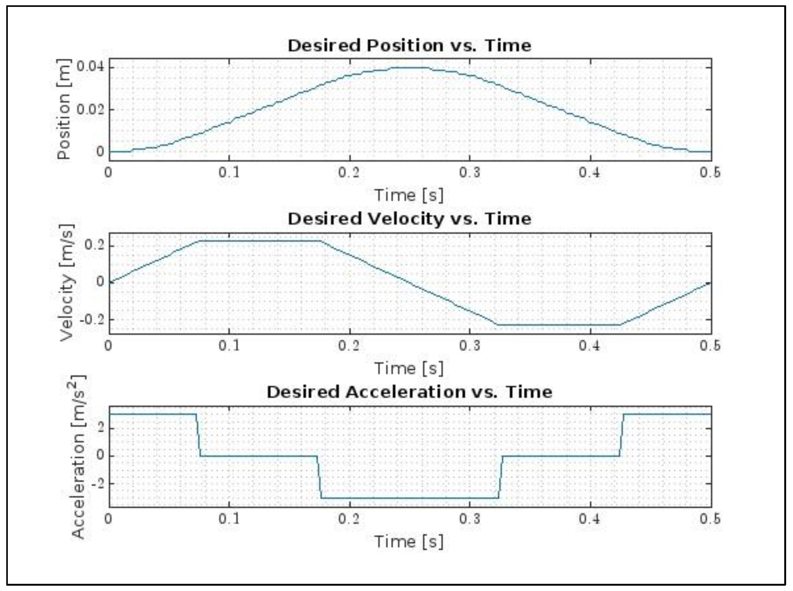
The input data are exported into the ‘Desired Trajectory’ function, which calculates trajectory profiles for acceleration, velocity, and position based on these inputs. In the trapezoidal trajectory profile, the stage accelerates during the first 12.5% of the cycle time, moves with a constant velocity between 12.5% and 37.5%, decelerates between 37.5% and 62.5%, moves with a constant velocity between 62.5% and 87.5%, and accelerates again for the final 12.5%. The resulting plots are shown in Figure 5.

The system’s effective moment of inertia is needed to calculate the torque profile corresponding to the desired trajectory. This is conducted through the function ‘Moment of Inertia’. After the effective moment of inertia is calculated, the desired trajectory’s torque profile is calculated in the function ‘Desired Torque’. Additionally, this function calculates the trajectory’s angular velocity profile. The resulting torque and velocity profiles are shown in Figure 6.

Before calculating the maximum possible trajectory the motor can execute, the torque–speed array is created in the ‘Motor Torque’ function. The user input data for this function include the desired torque level (here, peak torque is chosen), the rpm range (up to 3000 rpm), and whether the system experiences friction (included). The generated torque plot is shown in Figure 4.

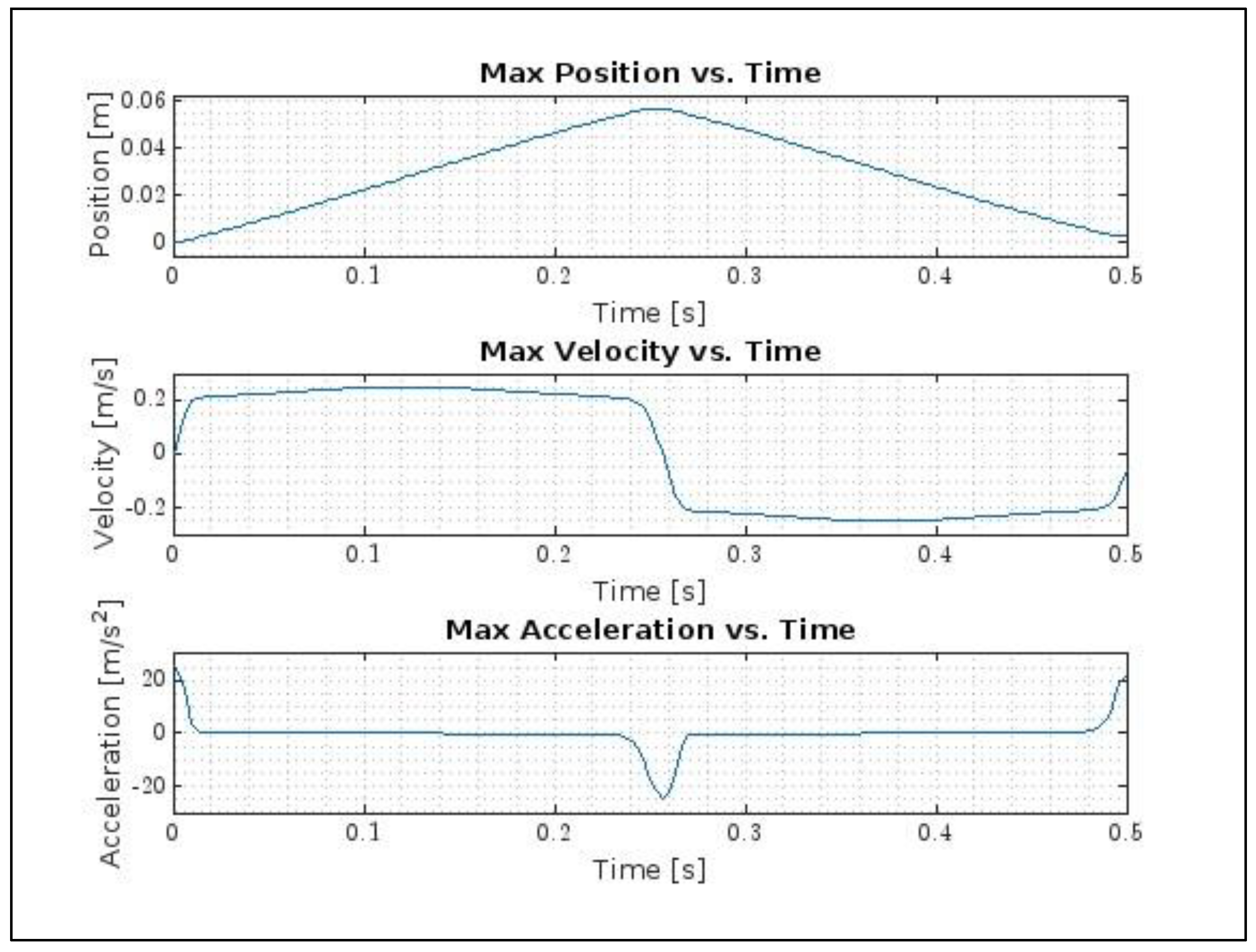
The ‘Max Trajectory’ function calculates the motor’s maximum possible performance based on user input for cycle rate and resolution, along with the effective moment of inertia and available motor torque. This calculation focuses on obtaining the maximum distance the motor can drive by continuously accelerating with its maximum available torque subject to time constraints. The process uses an iterative time-step approach. During each time increment, acceleration is calculated based on the effective moment of inertia and available torque at that speed. This acceleration is then integrated to update the velocity, and velocity and acceleration are used to determine the position. These updated position, velocity, and acceleration values become the starting conditions for the next time increment. Figure 7 and Figure 8 present the results, including acceleration, velocity, position, torque, and rpm (which correlate directly to velocity).

The next step in the program is a decision point. At this stage, the program checks if the maximum RPM value of the desired trajectory is lower than the maximum RPM the motor can achieve (in this case, 3000 RPM). Since the maximum RPM in the desired trajectory is 2750 (see the lower panel in Figure 6), which is slightly less than 3000 RPM, the ‘Real Torque’ function is called. This function compares the desired torque profile (torque over time) to the motor’s maximum torque profile (torque over RPM). If, at any time increment, the desired torque (corresponding to a given RPM) exceeds the motor’s maximum available torque, the ‘Real Torque’ value at that increment is capped at the motor’s maximum torque. Figure 9 illustrates the resulting torque over time and RPM over time plots.

The calculated real torque over time results (from Figure 9) are used in the final function call, ‘Real Trajectory’, to calculate the corresponding trajectory over time increments iteratively. The function reads the torque values and calculates the acceleration based on the given effective moment of inertia. This acceleration is then integrated to determine the velocity, which is subsequently integrated to obtain the position. These steps are repeated over the 200-time increments (nodes) to generate the resulting trajectories based on the real (maximum) torque values. Figure 10 illustrates these.

The final resulting trajectory has a displacement of 3.6 cm, lower than the desired displacement of 4 cm. However, the motor can achieve this trajectory as it considers the motor torque–speed characteristics and the inertia and damping in the system. This example illustrated obtaining an achievable trajectory based on a desired trajectory by computing the maximum performance and adjusting the desired trajectory according to the maximum possible trajectory. This process, aimed at optimizing motor performance, has been effectively executed.

4. Implementation and Testing

A simplified version of the developed methodology was implemented on a single-axis ball screw stage (see Figure 11) driven by an integrated servo motor (Clearpath SCHP 3426) from Teknic, Inc. (Victor, NY, USA). This stage is constructed like the model shown in Figure 2. The labeled components of the experimental setup, as shown in Figure 11a, are as follows. The motor (1) is the integrated servo motor that drives the ball screw. The ball screw (2) converts the motor’s rotational motion into linear motion to move the platform along its trajectory. The platform (3) is the moving component of the stage, designed to carry loads during testing procedures. The linear guides (4) ensure a smooth and precise motion by supporting the platform throughout its movement. Finally, the frame (5) serves as the structural base, maintaining alignment and providing stability to all the system components.

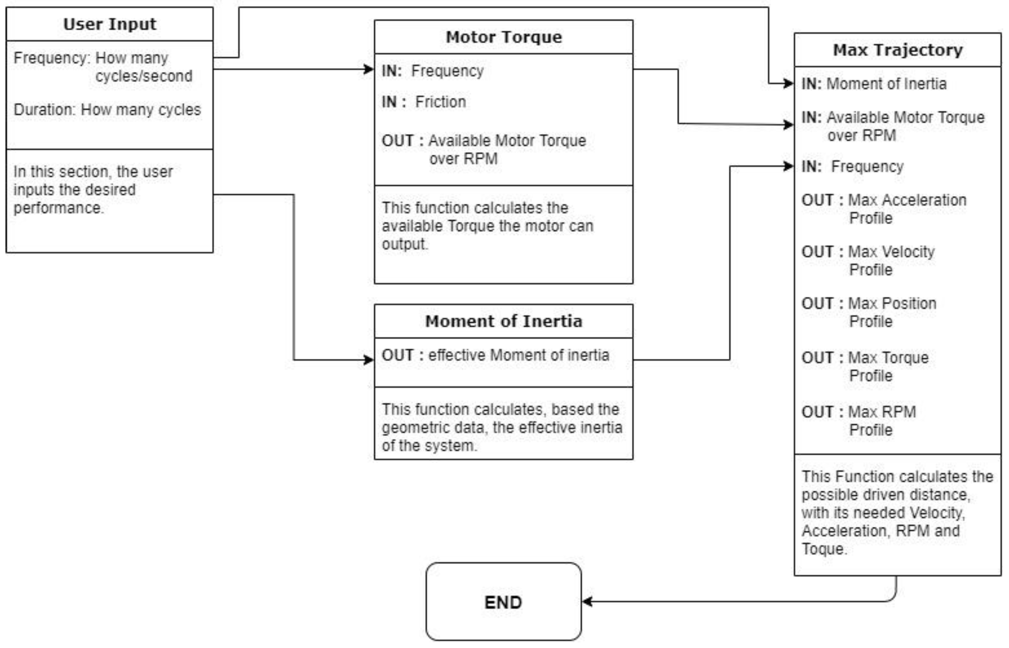
Integrated servo motors are available in several different types. A common type uses simple digital signals from switches, buttons, or sensor outputs to run the motor in various operation modes to control the motor’s position, velocity, or torque. A limitation of this motor type is that arbitrary motor displacements and motor parameters such as acceleration or velocity limits cannot be specified during program execution but have to be manually set during servo configuration. Another type, which is the one used in this work, is controlled using software API. This type allows motor displacement and parameters, such as acceleration or velocity limits, to be set or changed during program execution. However, even with the provided software, the user cannot specify any arbitrary trajectory or the desired travel time. The user sets the motor’s velocity and acceleration limits and the desired displacement, and the motor control software automatically generates either a triangular or trapezoidal velocity profile to satisfy the given displacement and motor performance. We have developed a testing methodology to work with this system limitation, ensuring the validity of the results. The simplified method is shown in Figure 12. In this approach, the user specifies the desired cycle rate for the motion. The algorithm computes the fastest trajectory that matches this rate and the resulting displacement of the device using this rate. The trajectory planner also outputs the maximum velocity and acceleration during the motion. To test this algorithm on the hardware, the cycle rate is manually adjusted to obtain specific displacements, such as the ones listed in

Table 2. Simulated and measured frequencies as a function of travel distance with no load applied to the platform.

Disp. (cm)	Simulated Frequency (Cycles/s)	Measured Frequency (Cycles/s)	Frequency Difference (Cycles/s)	% Diff.	Disp. (Encoder Counts)	Acceleration Limit (rpm/s)	Velocity Limit (rpm)
1.5	6.29	5.75	0.54	9.4	19,200	299,880	3000
2	4.92	4.7	0.22	4.7	25,600	299,880	3000
2.5	4.06	3.9	0.16	4.1	32,000	299,880	3000
3	3.46	3.4	0.06	1.8	38,400	299,880	3000
3.5	3.03	3	0.03	1.0	44,800	299,880	3000
4	2.69	2.7	−0.01	−0.4	51,200	299,880	3000
5	2.22	2.2	0.02	0.9	64,000	299,880	3000
7.5	1.56	1.55	0.01	0.6	96,000	299,880	3000
10	1.22	1.2	0.02	1.7	128,000	299,880	3000

. These displacements are fed to the actual hardware, and the cycle rate of the resulting motion is read from the hardware setup. These details are discussed in the next section. A Raspberry Pi was used as the control computer, and code written in C served as the control interface for the integrated servo motor. The code performed the following functions: (1) read user-defined input parameters such as the number of cycles and cycle rate; (2) compute the trajectory using the introduced methodology, including performance limits and outside parameters; (3) communicate with the servo motor via the motor’s software API to execute the calculated motion; and (4) wait for the response of the system to the programmed trajectory. The code used iterative algorithms to adjust motion parameters dynamically and ensured that motor torque–speed constraints were respected during execution.

Table 1 shows the system parameters used to model the stage. Table 2 outlines the displacements applied to the device. As mentioned, the trajectory planner determines the maximum possible motion rates for various displacements and loads. The motion rates were obtained iteratively by manually adjusting the frequency (cycles/second) until it matched each displacement case shown in Table 2.

5. Results and Discussion

The obtained results from the simplified trajectory planner are shown in Figure 13. The graph shows the relationship between travel distance (in cm) and frequency (cycles per second) for the linear motion device. As the travel distance increases, the displacement frequency decreases, which is typical for mechanical systems, where increased displacement often results in slower cycles due to factors like inertia and damping. The simulation results also show that the load applied to the device does not have much effect on the cycle rate in this ball-screw-driven system, as the ball screw significantly reduces the effective inertia seen by the motor due to loads applied to the platform.

To determine the system’s performance on the actual system, we have used the development software (ClearView from Teknic) that the motor manufacturer provides to view and measure the system’s response. Figure 14 displays a typical screen output from the software. The control software for the motor was run with the different displacement cases shown in Table 2, and the actual motion frequency of the device was read from the ClearView oscilloscope with an estimated accuracy of ±0.025 cycles/second. In the ClearView interface, the ‘Move Generator’ block is set to ‘Back and Forth Motion’ (analogous to the developed approach). The driven distance (in encoder counts units) is set to correspond to each of the motion cases tested. For example, a driven distance of 19,200 counts is equivalent to 15 mm as the encoder resolution is 6400 counts per revolution. The motor velocity limit is set at 3000 rpm, and the motor acceleration limit is set at 299,880 rpm/s (which corresponds to the acceleration for the selected motor when peak torque is applied). A dwell time of 1 ms is used after every full motion cycle (as 0 ms cannot be inputted), but the inaccuracy due to this should be insignificant. Each gray column on the oscilloscope represents 500 ms, with one full cycle represented by one full square wave. The plot shown in Figure 14 shows that the measured motion frequency is 5.75 cycles/s, determined by counting 11.5 cycles over two seconds, considering the estimated accuracy.

Table 2 lists the simulated and measured frequencies as a function of the travel distance in cm for the case of no load applied to the platform. The data are also plotted in Figure 15. The table also includes the acceleration limit based on peak-rated torque usage, the distance in counts for motor control, the motor’s maximum speed, and the resulting difference between the simulated and experimental frequencies. The resulting frequency differences indicate that the overall discrepancy is relatively low, especially at higher displacements and lower frequencies, with some differences falling within the readout accuracy of ±0.025 cycles/s. A sufficient alignment between the experimental and simulated frequencies was observed in the 3.0 to 1.2 cycles/s range.

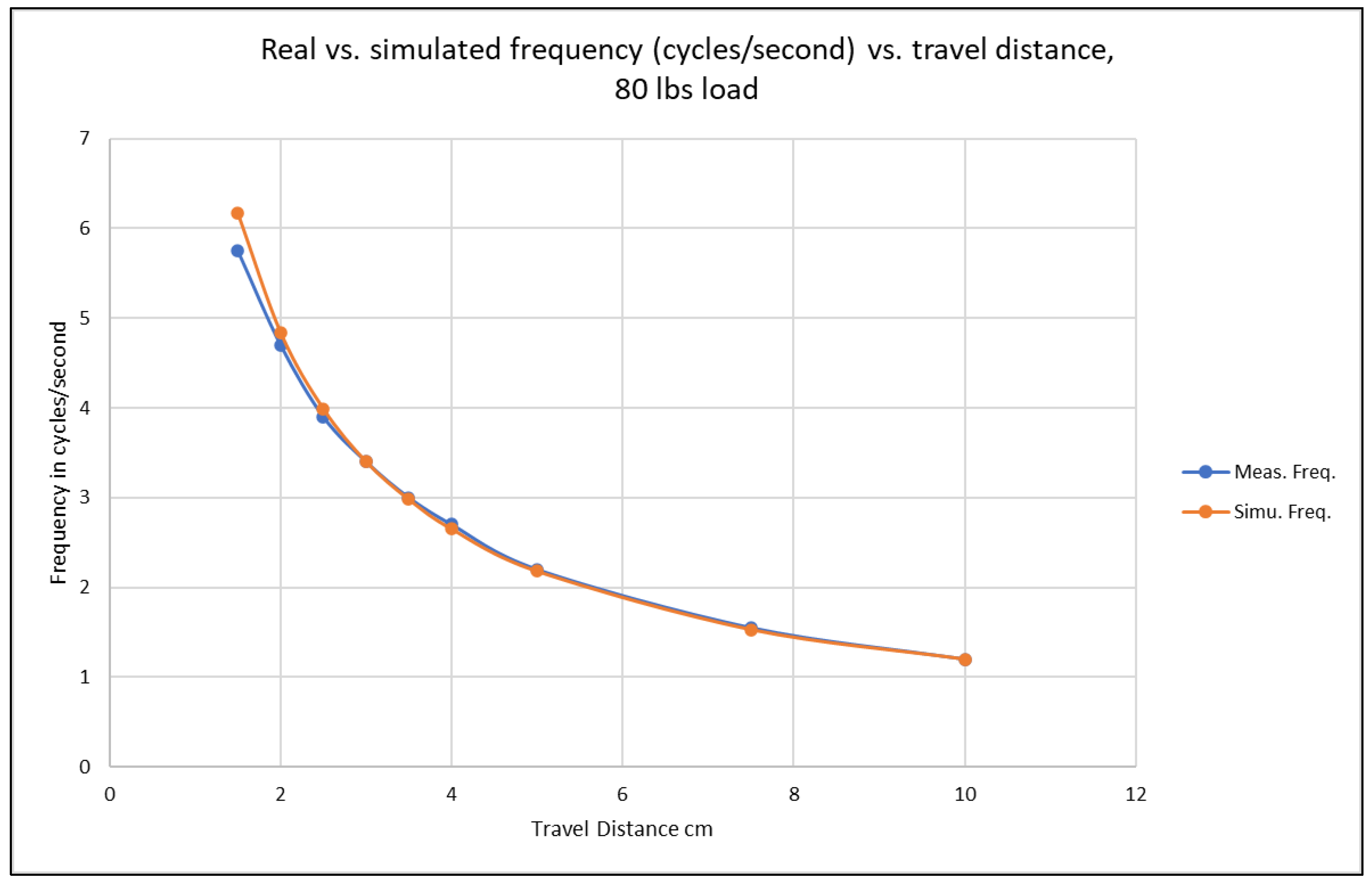
Figure 15 visually shows this relatively high accuracy/low discrepancy. Similar results were obtained for the 40 and 80 lb loads applied to the platform, and Figure 16 and Figure 17 show the simulated and measured frequencies for the 40 and 80 lb cases, respectively.

Similarly to the simulation results, the measured cycle frequency is inversely proportional to the travel distance, since a larger displacement will require more time to complete one cycle given that the acceleration is limited. In all the loading cases, there is a good agreement between the simulated and measured frequencies for cycle rates below three cycles/s. As the cycle rate increases, the discrepancy between the two becomes pronounced but still below 10% for the highest frequency. This discrepancy is due to two factors. One is the inaccuracy in reading the data from the scope (readout error of about 0.025 cycles/s), and the second is due to damping effects since, in actual systems, damping factors are more pronounced at higher frequencies and may not be fully captured in the simulation model.

We compare our approach to references [15,16,17,18], which target 1-DoF mechatronic systems. In our approach, we keep the trajectory time constant corresponding to a given cycle rate but vary the acceleration and velocity along the trajectory. Dona’ et al. [17] and Wang et al. [18] also keep the trajectory time constant, aligning with the approach presented in this work. In contrast, Fabris et al. [15] and Carabin and Vidoni [16] allow trajectory time to vary dynamically as part of the optimization process. Our approach uses iterative calculations to refine trajectory parameters, similar to those in Wang et al.’s [18] and Fabris et al.’s works [15]. This contrasts with the analytical or direct methods used by Dona’ et al. [17] and Carabin and Vidoni [15], which rely on closed-form analytical solutions without iterative refinement.

The approach we developed has some limitations. The iterative calculation of trajectories requires more computational resources than traditional pre-programmed approaches, which could be challenging for real-time applications with minimal hardware. Additionally, while the methodology accounts for system dynamics, it requires accurate input parameters for loads and inertia to maintain its predictive accuracy, a challenge also noted in high-speed manipulator trajectory planning. Finally, the method assumes detailed knowledge of motor characteristics, which may only sometimes be readily available, as highlighted by Hu et al. [13].

6. Conclusions

This paper presents a practical methodology for developing motion trajectories for the reciprocating motion of a single-axis device. The versatile method explicitly incorporates motor torque–speed constraints into trajectory planning and can be implemented on various devices. For devices in which the control software allows for trajectory modification, the methodology starts with a given desired trajectory, such as triangular or trapezoidal, that the user creates based on specifying the desired displacement and the cycle rate for back-and-forth motions. Using a dynamic model of the device and the torque–speed characteristics of the motor, the methodology iteratively modifies the starting trajectory to produce one that does not violate the given motor torque–speed specifications and maintains the specified trajectory time. For devices driven by integrated servosystems, in which the control software for these motors does not allow the user to select any arbitrary trajectory or the desired travel time, the methodology computes the maximum cycle rate for back-and-forth motions.

The methodology was demonstrated through a simulation example. A simplified version requiring minimal input data was also implemented on a prototype device using an integrated servo motor to drive a ball screw stage. Tests were performed at various motion rates and loads. The experimental results showed strong agreement between the predicted and measured motion rates, particularly for rates below three cycles per second. These findings suggest that the proposed methodology is a valuable tool for predicting the performance of systems utilizing integrated servo motors in reciprocating motion applications.