Article

Dynamic Response of Electromechanical Coupled Motor Gear System with Gear Tooth Crack

1
College of Mechanical Engineering and Automation, Huaqiao University, Xiamen 361021, China
2
Fujian Key Laboratory of Green Intelligent Drive and Transmission for Mobile Machinery, Xiamen 361021, China
3
Department of Mechanical Engineering, Ostfalia University of Applied Sciences, 38302 Wolfenbüttel, Germany
*
Author to whom correspondence should be addressed.
Machines 2024, 12(12), 918; https://doi.org/10.3390/machines12120918
Submission received: 25 October 2024 / Revised: 6 December 2024 / Accepted: 11 December 2024 / Published: 15 December 2024
(This article belongs to the Section Electrical Machines and Drives)

Abstract

The motor gear system (MGS) is recognized for its potential in enhancing transmission efficiency and optimizing space utilization. However, the system is subjected to challenges, notably the occurrence of abnormal vibrations. These issues stem from the dynamic interaction between the motor and gears, the presence of nonlinear factors in gear system, and the impact of gear faults, all of which contribute to complex vibration patterns. Traditional dynamic models have been found to be inadequate in effectively addressing the complexities associated with electromechanical coupling problems in MGS. To address these limitations, a comprehensive analysis approach is proposed in this paper, which is grounded in the development of an electromechanical coupling model. This method involves establishing a coupled dynamic model of the motor and gear system, integrating numerical simulations, and experimental validations to thoroughly analyze the vibration characteristics of the system. Through this multifaceted methodology, a detailed analysis of the system’s vibration characteristics is conducted. The results indicate that internal excitations from tooth root cracks not only directly affect dynamic characteristics of the gear transmission system (GTS) but also indirectly influence dynamic behavior of the motor, which offers valuable insights into modeling integrated MGS and provides significant solutions for fault diagnosis within these systems.

1. Introduction

The motor gear system (MGS) is extensively employed across industrial, transportation, and agricultural sectors, owing to its high efficiency, stability, substantial torque, and precision. As efforts to enhance the efficiency, integration, and reliability of drive systems continue, MGS is increasingly moving towards more complex structures. However, this evolution introduces new challenges [1,2]. In particular, the electromechanical coupling dynamics and fault prediction within MGS necessitate comprehensive investigation.
With the development of integrated MGS, dynamic interaction issues between mechanical and electrical systems have emerged. For instance, the performance of the mechanical system is influenced by the current and voltage signals, as well as the control systems within the Electrical Drive System (EDS). Conversely, it has been observed that vibrations, shocks, and mechanical loads exert an influence on the stability of the electrical system, which has been found to contribute to the reduction in the lifespan of electrical components [3,4]. Szolc et al. [5] investigated the dynamic electromechanical coupling between the motor and gear transmission system (GTS) of rotating machinery, revealing that electromagnetic stiffness and damping coefficients are influenced not only by the motor but also gears. Liu et al. [6] developed a dynamic model for an off-grid switched-reluctance wind turbine hydrogen production system, incorporating both mechanical and electromagnetic features. Chen et al. [7] addressed the strong coupling between gear and generator systems, which influences resonance speed and vibration signals, highlighting the importance of studying these interactions for safe drivetrain operation and design. Jiang et al. [8] studied the electromechanical coupling characteristics of coal mining machinery, considering both the electromagnetic effects and bending-torsional vibration characteristics of permanent magnet synchronous motor (PMSM). Kumar [9] introduced an electromechanical model for a single-stage gearbox with gear tooth root cracks, and developed using a modified Lagrangian approach and incorporating Rayleigh dissipative potential. Drawing upon the literature review, it is evident that both the EDS and GTS exhibit abnormal nonlinear vibrations as a result of internal electromechanical coupling.
To study the electromechanical coupling dynamic characteristics of MGS, it is essential to establish an accurate electromechanical coupling dynamic model [10,11]. Hao et al. [12] developed a mathematical model to assess the reliability of GTS and subsequently designed a digital platform to facilitate rapid reliability modeling. In a related study, Zhang et al. [13] proposed a design theory and method aimed at achieving high power density in heavy-duty GTS, particularly those operating under complex loads. To optimize gear parameter design, Zhou et al. [14] explored the effects of friction, impact, and lubrication on gear dynamics. Jedliński [15] examined eccentricity and backlash in spur gears using a 26-degree of freedom model of GTS. Bartelmus [16] explored the application of mathematical modeling and computer simulation to enhance gearbox diagnostic inference during monitoring. In a subsequent study, Sakaridis [17] investigated the impact of individual tooth inertia on spur gear dynamics, proposing a model that distinguishes tooth inertia from the gear body and introduces an innovative method for analyzing tooth contact. However, the prevalent use of local model in MGS frequently neglects the interaction between electrical and mechanical systems, leading to inaccurate simulation outcomes [18,19]. Therefore, the establishment of a comprehensive dynamic model is imperative to facilitate effective multi-domain electromechanical coupling studies.
The introduction of electromechanical coupling in MGS has been observed to exacerbate vibrational phenomena, thereby presenting both novel challenges and opportunities within the domain of fault diagnosis [20]. Addressing the challenge of real-time monitoring of equipment faults in mining machinery, Lu and Zhang [21] investigated the motor current response of mining equipment due to gear tooth root crack faults, and proposed a feasible method to predict mechanical faults by monitoring motor current. Ge [22] assessed the resonance risk by analyzing torsional vibrations at resonant speed, which are identifiable through current signals. Marzebali [23] studied how torsional vibrations affect electrical signals in a complex system, highlighting challenges in detecting gearbox frequencies. Kumar [24] modeled the electromechanical behavior of a straight bevel gear pair under various fault conditions, including healthy, chipped, and missing teeth. Han [25] proposed a motor current model for diagnosing localized defects in planet rolling bearings, which includes a dynamic analysis of a motor-driven planetary gearbox system. Ouyang [26] found that by analyzing gear characteristics in both time and frequency domains, accurate diagnosis of gear status is possible. Molaie [27] analyzed the dynamics of spiral bevel gears, accounting for torsional stiffness, time-dependent stiffness, and backlash, validating the model with a single-degree-of-freedom system. Sang et al. [28] investigated the lateral synthetic vibration signals and output torsional vibration signals of the motor-3K planetary gear system, which analyzed the feasibility of using these two vibration signals for fault diagnosis. Chai et al. [29] utilized the motor driver as an intelligent sensor, leveraging signals such as current and motor speed obtained from the drive system as fault carriers to monitor and diagnose the states of GTS. Yousfi et al. [30] effectively detected gear tooth faults using vibration and motor current signature analysis in both time and frequency domains, demonstrating satisfactory responses under faulty conditions. Sheng et al. [31] proposed a dynamic model of MGS aimed at acquiring motor current and gear fault data. Chen et al. [32] proposed a calculation method for the time-varying mesh stiffness and analyzed its coupling effects with rail transit trains. Ottewill [33] extended the application of the synchronous signal averaging method, traditionally employed for diagnosing tooth faults in parallel shaft gearboxes, to include the monitoring of tooth faults in epicyclic gearboxes. To maintain high precision in MGS, continuous monitoring of gear fault behavior is essential.
Research on the dynamics of electromechanically coupled systems in motor gear systems (MGS) has achieved significant progress. However, several persistent challenges have been identified, including the development of models that exhibit insufficient accuracy, inadequate consideration of electromechanical coupling factors, and the inherent difficulties associated with monitoring tooth root crack faults. As a result, achieving a comprehensive understanding of the dynamics and fault diagnosis within electromechanically coupled systems of mechanical gearboxes (MGS) is of paramount importance. The availability of accurate models is essential for optimizing system design, minimizing failure rates, and enhancing overall performance. Nevertheless, existing models frequently neglect critical dynamic aspects and the intrinsic complexity of the system. In response to these issues, an improved MGS model that effectively balances accuracy and computational efficiency is presented. This proposed model is intended to support design optimization and facilitate effective fault diagnosis within the system.

2. Electromechanical Coupling Modeling of MGS

Figure 1 illustrates the basic structure of the MGS, which includes a three-phase permanent magnet synchronous motor (PSMS) as drive motor, gearbox, and load. Inside the gearbox, there is a spur gear, with both ends of the parallel shafts supported by rolling bearings. The motor is connected to the input shaft of the gearbox, and the load is connected to the output shaft, both via couplings.
The power transmission and coupling relationships between the subsystems of MGS are depicted in Figure 2. The improved model encompasses the motor control, electronic, motor rotor, GTS, and load, explicitly considering the coupling interactions between these subsystems. Here, ui represents voltage signals, ii current, [X Y θ] displacement/vibration, ωi the angular velocity, Fi force, and Ti torque. The modeling of these subsystems will be introduced in detail below.

2.1. Equivalent Circuit Model of PMSM

In this section, the mathematical model of three-phase PMSM is established. The voltage equations and flux linkage equations of motor in stationary coordinate are detailed as follows [34]
u a b c = R i a b c + d d t ψ a b c s ψ a b c s = L a b c i a b c + ψ a b c r
where uabc is voltage vector of stator windings, iabc current vector of stator windings, ψ a b c s flux linkage vector of stator windings, ψ a b c r flux linkage vector of rotor windings, Labc inductance matrix of stator windings, ϕf flux linkage of permanent magnet, θe angle of rotor electric, and R resistance of stator windings.
The model of PMSM in stationary coordinate exhibits time-varying and coupling characteristics. To facilitate the design of the subsequent controller, a mathematically decoupled model is established under the d-q frame [34]. The stator voltage equation in the d-q frame is
u d = R i d + i d d L d ( i d ,   i q ) d t + d ϕ f ( i d ,   i q ) d t           ω e L q ( i d ,   i q ) i q u q = R i q + i q d L q ( i d ,   i q ) d t + L q ( i d ,   i q ) d i q d t           + ω e ( L d ( i d ,   i q ) i d + ϕ f ( i d ,   i q ) )
The stator flux linkage equations in the d-q frame are
ϕ d = L d i d + ϕ f ϕ q = L q i q
Let [ud uq] be the d-axis and q-axis components of stator voltage, respectively. Similarly, [id iq] are the d-axis and q-axis components of stator current, [ϕd ϕq] the stator flux linkage, [Ld Lq] the inductance, ωe the electrical angular velocity, and ϕf the flux linkage of permanent magnet. The electromagnetic torque equation is expressed
T e = 3 2 n p i q i d L d ( i d ,   i q ) L q ( i d ,   i q ) + ϕ f ( i d ,   i q )
In addition, it is important to note the following relationships
ω e = d d t θ e ,   ω m = ω e n p ,   n = 30 π ω m
where ωm is the mechanical angular velocity of motor, n the rotational speed of motor, and np the number of motor pole pairs. The differential equation governing the torsional motion of motor rotor, which incorporates rotor eccentricity, is expressed as follows:
( J + m e 2 ) θ ¨ m = T e T L B θ ˙ m + m e [ sin ( ω m t ) X ¨ cos ( ω m t ) Y ¨ ]
where X and Y are the transverse displacements of motor rotor, θm is the mechanical angular displacement of rotor, m the rotor mass, TL the load torque, B the electromagnetic damping coefficient, and e the eccentricity of rotor.
To derive the fundamental equations in the stationary reference frame, one must apply the inverse Park and Clarke transformations to the equations originally formulated in the synchronous rotating d-q reference frame [34].

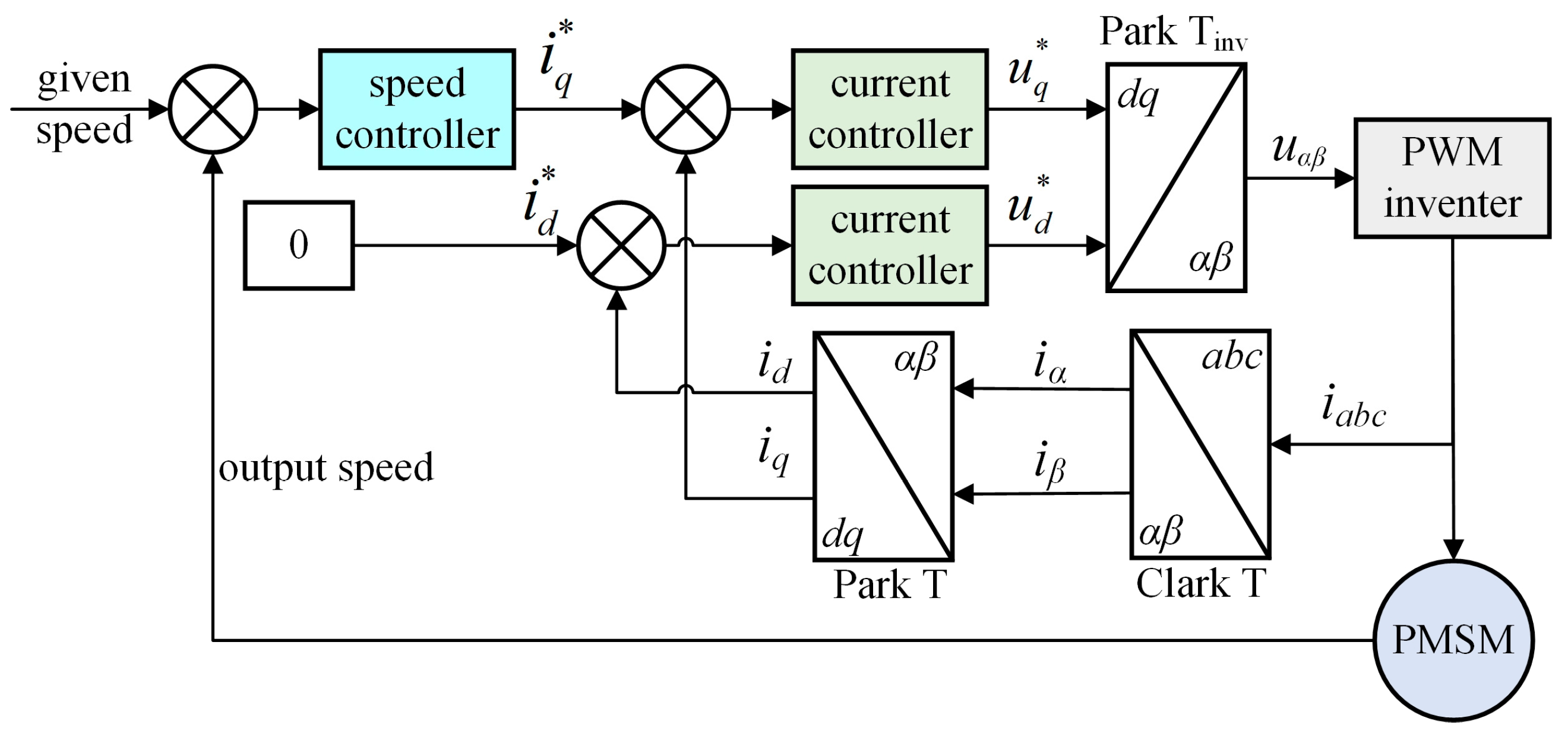
2.2. Vector-Control of Motor

Research frequently overlooks the effect of motor control technology on MGS, neglecting factors such as parameter errors and external disturbances, which can lead to instability. This paper addresses these effects by incorporating motor control technologies into the analysis of GTS and EDS through an electromechanical coupling model. Figure 3 illustrates the control process flowchart, which comprises two primary modules: the speed controller and the current controller. The paper introduces various control methods for designing these controllers, including the Proportional–Integral (PI) speed controller, PI current controller, and Sliding Mode Control (SMC) speed controller.
(1)
Review of PI speed controller
The PI speed controller, a widely adopted technique in industry, reduces stability errors by adjusting proportional gain based on the deviation between actual and desired speeds [35]. Further details are below.
i q * = K P e + K I e d t
where e = ωrefω, and KP, KI are control parameters.
(2)
Review of PI current controller
Employing a conventional PI controller in conjunction with feedforward decoupling control, the voltage in the q-d frame is derived by analytic derivation.
u d * = K p d + K i d s i d * i d ω e L q i q u q * = K p q + K i q s i q * i q + ω e L d i d + ψ f
The closed-loop transfer function of the system using PI controller is defined as follows [36].
G c ( s ) = G ( s ) C ( s ) F ( s ) = [ I C ( s ) G ^ ( s ) ] 1 C ( s ) C ( s ) = G 1 ( s ) L ( s )
where L ( s ) = α I / ( s + α ) , α is the design parameter, which is positive. Then,
F ( s ) = α L d + R s 0 0 L q + R s
By combining Equations (9) and (10), we obtain
G c ( s ) = α s + α I
Comparing Equation (11) with Equation (8) shows that controller tuning parameters are reduced from 2 to 1, simplifying the process. This adjustment fulfills the following relationship
K p d = a L d K i d = a R K p q = a L q K i q = a R  
The rise time (TR), defined as the time taken for the system to transition from 10% to 90% of its step response, is approximately given by TR = ln9/α. Lowering the value of α extends the response time, whereas increasing α hastens it. However, the value of α is constrained by the electrical time constant. In this study, α is set to 1500.
(3)
Review of SMC speed controller
Setting the id to zero aligns with the rotor magnetic field, which is conducive to achieving better control in surface-mounted PMSM. The mathematical model detailed in Section 2.1 is subsequently represented in the q-d reference frame.
d i q   d t = 1 L s R i q p n ψ f ω m + u q d ω m d t = 1 J T L + 3 p n ψ f 2 i q B ω m
The state variable of speed controller is
x 1 = ω ref ω m x 2 = x ˙ 1 = ω ˙ m
Derivation of Equation (14),
x ˙ 1 = ω ˙ m = 1 J T L 3 p n ψ f 2 i q + B ω m x ˙ 2 = ω ¨ m = 3 p n ψ f 2 J i ˙ q B x 2
Let u = i ˙ q , D = 3 p n ψ f 2 J , and rewrite Equation (15) as
x ˙ 1 x ˙ 2 = 0 1 0 1 x 1 x 2 + 0 D u
The sliding surface is given
s = c x 1 + x 2 s ˙ = c x ˙ 1 + x ˙ 2 = c x 2 + x ˙ 2 = ( c 1 ) x 2 D u
where c > 1, and the exponential reaching law is adopted
s ˙ = K 1 sgn ( s ) K 2 s
where K1 and K2 are the parameters of SMC. Combining Equations (17) and (18)
u = 1 D ( c 1 ) x 2 + K 1 sgn ( s ) + K 2 s
The stability of SMC controller is verified using a Lyapunov function.
V ˙ = s s ˙ = s ( c 1 ) x 2 D u       = s ( c 1 ) x 2 ( c 1 ) x 2 + K 1 sgn ( s ) + K 2 s         = K 1 sgn ( s ) s K 2 s 2 0
K1sgn(s) and K2s2 are both positive, and V ˙ < 0 is negative definite. Thus, the system is asymptotically stable with SMC controller. Then, the reference current in q-axis is expressed as
i q * = 1 D 0 t ( c 1 ) x 2 + K 1 sgn ( s ) + K 2 s d τ
The inclusion of an integral term in controller serves not only to attenuate oscillations but also eliminate steady-state errors, thereby enhancing the overall control quality.

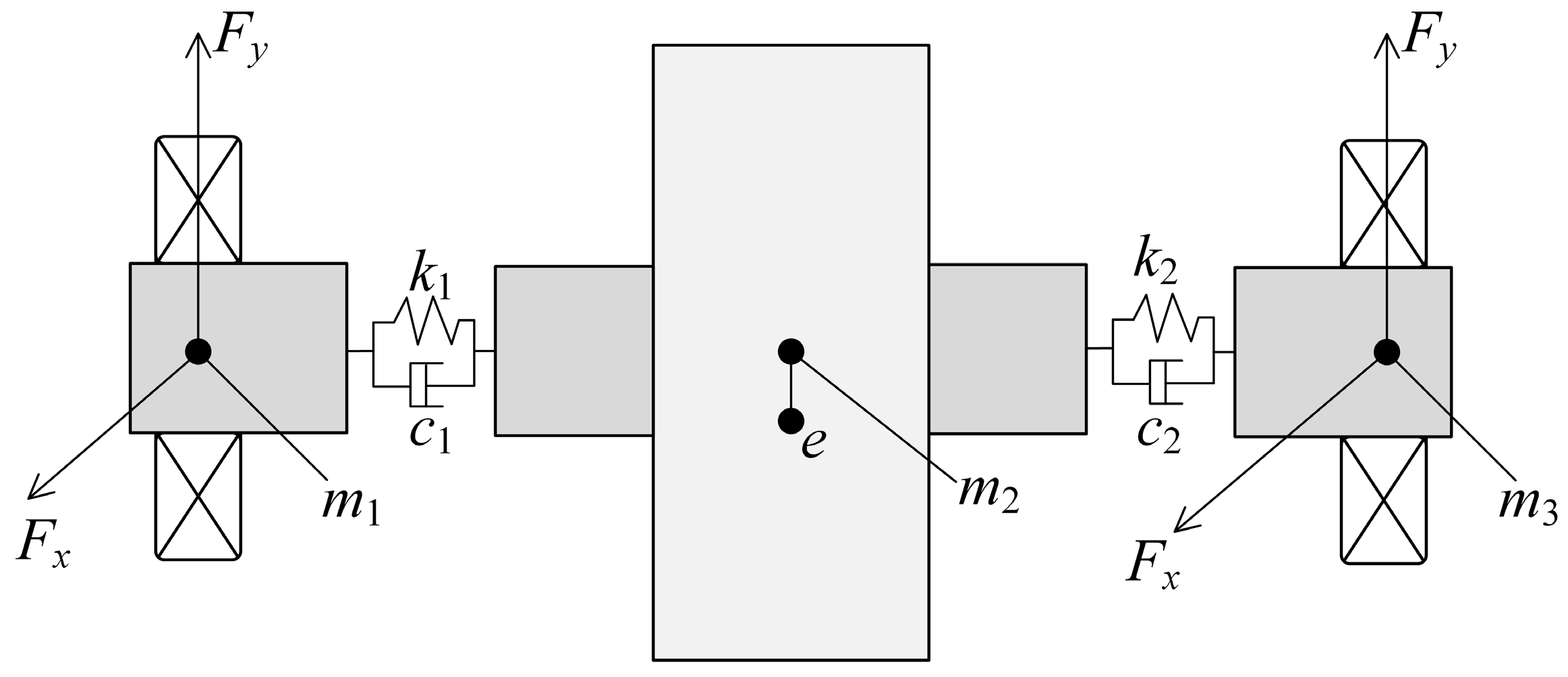
2.3. Mechanical Model of Motor Rotor

Based on the equivalent circuit model of PMSM, the interaction channel is established that links the torsional motion of the motor rotor with GTS, thereby forming an electromechanical coupling model. The coupling between the torsional and lateral vibrations is highlighted by Equation (6), indicating the necessity for incorporation of lateral vibration model. The traditional torsional model neglects these effects, which can influence the air gap, output torque, and noise. To address these issues comprehensively, a lateral vibration model is integrated with the equivalent circuit and torsional models of motor, resulting in an improved electromechanical coupling model.
The study employs the Jeffcott model [37] to analyze the dynamics of the motor rotor, as depicted in Figure 4. The model incorporates lateral vibration and the support forces of rolling bearings. Here, m1 is the mass at the left bearing support, m2 the rotor mass (same as m in Equation (6)), and m3 mass at the right bearing support. The bearing forces (Fx, Fy) can be calculated using the method outlined in reference [38].
The rotor vibrations are described by the mathematical model in the X-Y directions. Left bearing displacements are denoted as X1 and Y1, rotor center displacements as X2 and Y2 (same as X and Y in Equation (6)), and right bearing displacements as X3 and Y3.
m 1 X ¨ 1 + c 1 X ˙ 1 + k 1 X 1 X 2 = F x ( X ˙ 1 , Y ˙ 1 , X 1 , Y 1 ) m 1 Y ¨ 1 + c 1 Y ˙ 1 + k 1 Y 1 Y 2 = F y ( X ˙ 1 , Y ˙ 1 , X 1 , Y 1 ) m 2 X ¨ 2 + c 2 X ˙ 2 + k 1 X 2 X 1 + k 2 X 2 X 3 = m 2 e ω m 2 cos ω m t + β + F x U M P m 2 Y ¨ 2 + c 2 Y ˙ 2 + k 1 Y 2 Y 1 + k 2 Y 2 Y 3 = m 2 e ω m 2 sin ω m t + β + F y U M P m 3 X ¨ 3 + c 3 X ˙ 3 + k 2 X 3 X 2 = F x ( X ˙ 3 , Y ˙ 3 , X 3 , Y 3 ) m 3 Y ¨ 3 + c 3 Y ˙ 3 + k 2 Y 3 Y 2 = F y ( X ˙ 3 , Y ˙ 3 , X 3 , Y 3 )
where c1, c2, c3 represent the damping at shaft and disc, and k1, k2 the bending stiffness of shaft. The forces FyUMP and FyUMP denote the component forces of the unbalanced magnetic pull (UMP) in the X and Y directions, respectively. The magnetic lines passing through the stator and rotor are naturally shortened, generating a pull force. Uniform air gaps result in symmetrical pull forces on the rotor, leading to a net force of zero. However, rotor lateral displacement is observed to create non-uniform air gaps, causing radial unbalanced magnetic pull [37]. Consequently, Equation (22) integrates the UMP of the motor rotor, with the force calculation method detailed in the literature [39].

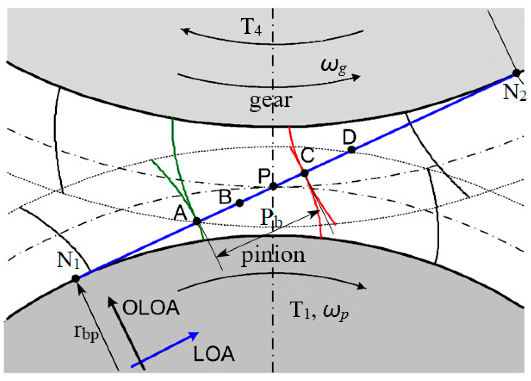
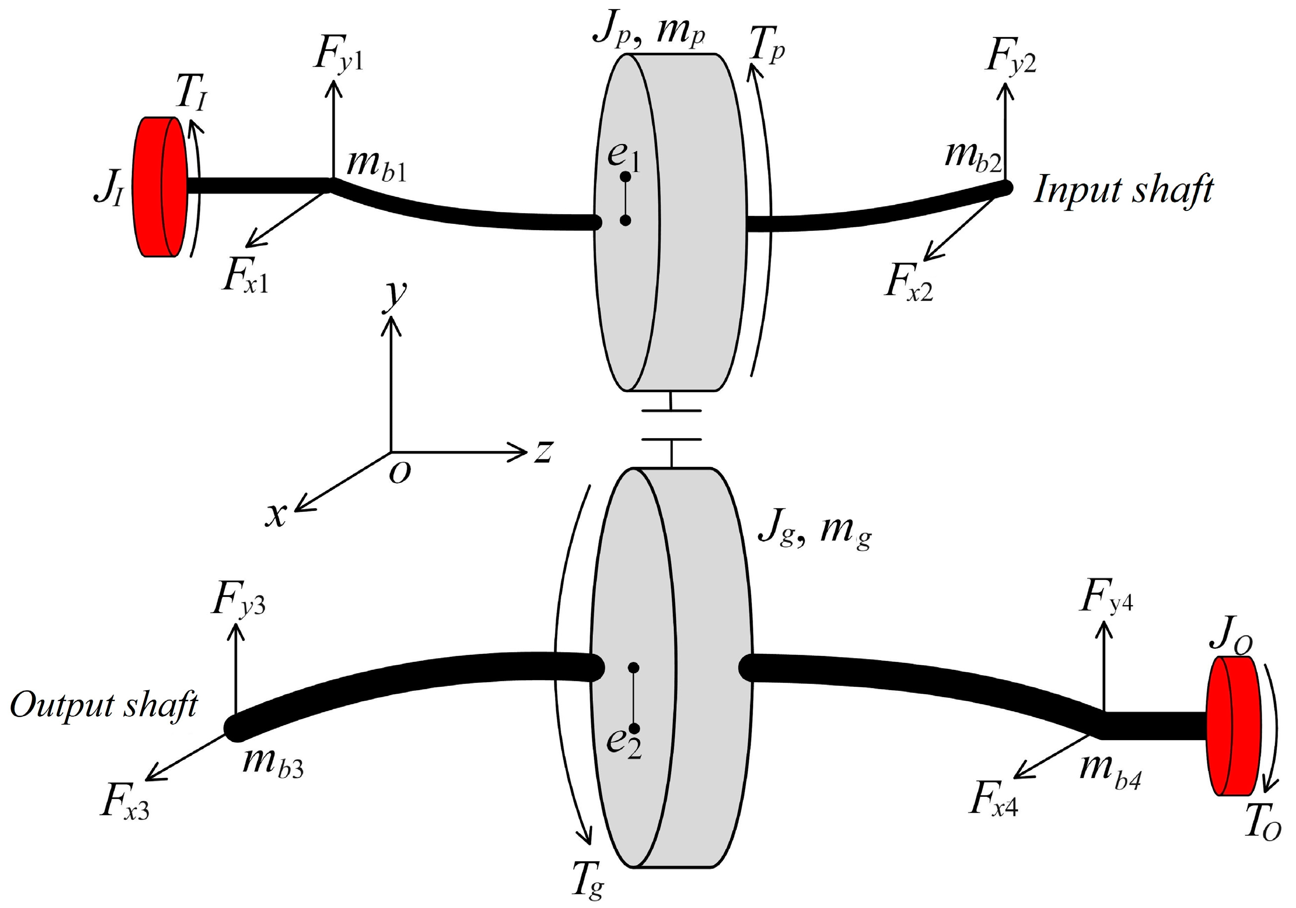
2.4. Dynamic Model of GTS

For precision equipment requiring operation with low vibrations, a more precise modeling method for GTS, named the Multibody of Gear-Rotor-Bearing System [40], is referenced. The model distinctly separates parallel shaft axes and their components, employing a gear tooth rigid body dynamics model to calculate the torque exerted on the hub by meshing gear teeth. This dynamic model, as illustrated in Figure 5, treats the hub as a disc on the shaft, with the gear meshing force represented as meshing torque.
In Figure 5, the input and output torques are denoted as TI and TO, respectively, where the subscript I represents the input and O represents the output. The bearing forces in the x and y directions for both the input and output shafts are labeled as Fxi and Fyi (i = 1~4), and the bearing masses are denoted as mbi. The mass of the gear hub is represented as mi (i = p/g), with the subscript p for pinion and g for gear, and their corresponding moments of inertia are Ji. ei is the gear eccentricity.
Equation (23) formulates the differential equation for the GTS of input shaft, whereas Equation (24) represents the corresponding system for the output shaft within the context of lateral torsional coupled vibration. The variable θi signifies the torsional angle displacement at each concentrated mass location, cbi the damping of bearing, ωi the shaft speed, ζi the dimensionless position parameter of gear hub. In this context, ζi is set to a value of 0.5. In Equations (23) and (24), c1 and k1 are the torsional damping and stiffness of shaft 1, while c2 and k2 are the lateral damping and stiffness of shaft 2. Similarly, c3 and k3 denote the lateral damping and stiffness of shaft 2, while c4 and k4 the torsional damping and stiffness of shaft 2.
J I θ ¨ I + c I θ ˙ I θ ˙ p + k I θ I θ p = T I m b 1 x ¨ b 1 + c b 1 x ˙ b 1 + ζ 2 c p ζ 1 x ˙ b 2 + ζ 2 x ˙ b 1 x ˙ p + ζ 2 k p ζ 1 x b 2 + ζ 2 x b 1 x p = F x 1 m b 1 y ¨ b 1 + c b 1 y ˙ b 1 + ζ 2 c p ζ 1 y ˙ b 2 + ζ 2 y ˙ b 1 y ˙ p + ζ 2 k p ζ 1 y b 2 + ζ 2 y b 1 y p = F y 1 m b 1 g J p + m p e 1 2 θ ¨ p + c I θ ˙ p θ ˙ I + k I θ p θ I = m p e 1 [ sin ( ω p t + θ P ) x ¨ p cos ( ω p t + θ p ) y ¨ p ] F n r b p ( F f p 1 s p 1 + F f p 2 s p 2 ) m p x ¨ p + c p x ˙ p ζ 1 x ˙ b 2 ζ 2 x ˙ b 1 + k p x p ζ 1 x b 2 ζ 2 x b 1 = m p e 1 [ ( ω p + θ ˙ p ) 2 cos ( ω p t + θ p ) + θ ¨ p sin ( ω p t + θ p ) ] + F f p m p y ¨ p + c p y ˙ p ζ 1 y ˙ b 2 ζ 2 y ˙ b 1 + k p y p ζ 1 y b 2 ζ 2 y b 1 = m p e 1 [ ( ω p + θ ˙ p ) 2 sin ( ω p t + θ p ) θ ¨ p cos ( ω p t + θ p ) ] m p g F n m b 2 x ¨ b 2 + c b 2 x ˙ b 2 + ζ 1 c p ζ 1 x ˙ b 2 + ζ 2 x ˙ b 1 x ˙ p + ζ 1 k p ζ 1 x b 2 + ζ 2 x b 1 x p = F x 2 m b 2 y ¨ b 2 + c b 2 y ˙ b 2 + ζ 1 c p ζ 1 y ˙ b 2 + ζ 2 y ˙ b 1 y ˙ p + ζ 1 k p ζ 1 y b 2 + ζ 2 y b 1 y p = F y 2 m b 2 g
m b 3 x ¨ b 3 + c b 3 x ˙ b 3 + ζ 4 c g ζ 3 x ˙ b 4 + ζ 4 x ˙ b 3 x ˙ g + ζ 4 k g ζ 3 x b 4 + ζ 4 x b 3 x g = F x 3 m b 3 y ¨ b 3 + c b 3 y ˙ b 3 + ζ 4 c g ζ 3 y ˙ b 4 + ζ 4 y ˙ b 3 y ˙ g + ζ 4 k g ζ 3 y b 4 + ζ 4 y b 3 y g = F y 3 m b 3 g J g + m g e 2 2 θ ¨ g + c O θ ˙ g θ ˙ O + k O θ g θ O = m g e 2 [ sin ( ω g t + θ g ) x ¨ g cos ( ω g t + θ g ) y ¨ g ] + F n r b g + ( F f g 1 s g 1 + F f g 2 s g 2 ) m g x ¨ g + c g x ˙ g ζ 3 x ˙ b 4 ζ 4 x ˙ b 3 + k g x g ζ 3 x b 4 ζ 4 x b 3 = m g e 2 [ ( ω g + θ ˙ g ) 2 cos ( ω g t + θ g ) + θ ¨ g sin ( ω g t + θ g ) ] + F f g m g y ¨ g + c g y ˙ g ζ 4 y ˙ b 4 ζ 4 y ˙ b 3 + k g y g ζ 3 y b 4 ζ 4 y b 3 = m g e 2 [ ( ω g + θ ˙ g ) 2 sin ( ω g t + θ g ) θ ¨ g cos ( ω g t + θ g ) ] m g g + F n m b 4 x ¨ b 4 + c b 4 x ˙ b 4 + ζ 3 c g ζ 3 x ˙ b 4 + ζ 4 x ˙ b 3 x ˙ g + ζ 3 k g ζ 3 x b 4 + ζ 4 x b 3 x g = F x 4 m b 4 y ¨ b 4 + c b 4 y ˙ b 4 + ζ 3 c g ζ 3 y ˙ b 4 + ζ 4 y ˙ b 3 y ˙ g + ζ 3 k g ζ 3 y b 4 + ζ 4 y b 3 y g = F y 4 m b 4 g J O θ ¨ O + c O θ ˙ O θ ˙ g + k O θ O θ g = T O
in which, the meshing forces Fn are expressed as
F n = k ( t ) f ( r b p θ p r b g θ g + y p y g e ( t ) ) + c ( t ) ( r b p θ ˙ p r b g θ ˙ g + y ˙ p y ˙ g e ˙ ( t ) )
Here, k(t) denotes the Time-Varying Meshing Stiffness (TVMS), and f(x) represents a discontinuous function of the gear along the mesh line. In addition, the frictions experienced by the pinion and gear are denoted by Ffi (where i = p for the pinion and i = g for the gear). The moment arms for these friction forces on the pinion and gear are represented by spi and sgi, respectively (where i = 1, 2 corresponds to the meshing tooth pairs). Detailed descriptions of these nonlinear parameters are provided in the Appendix A.

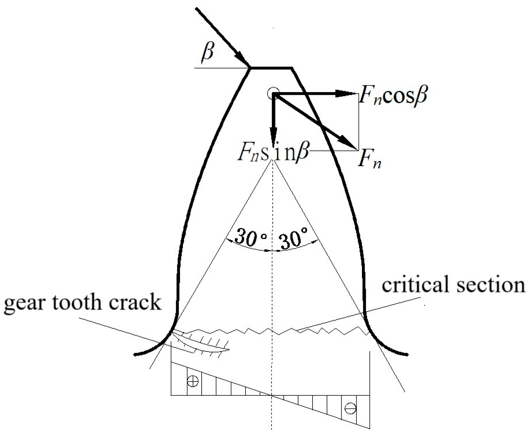
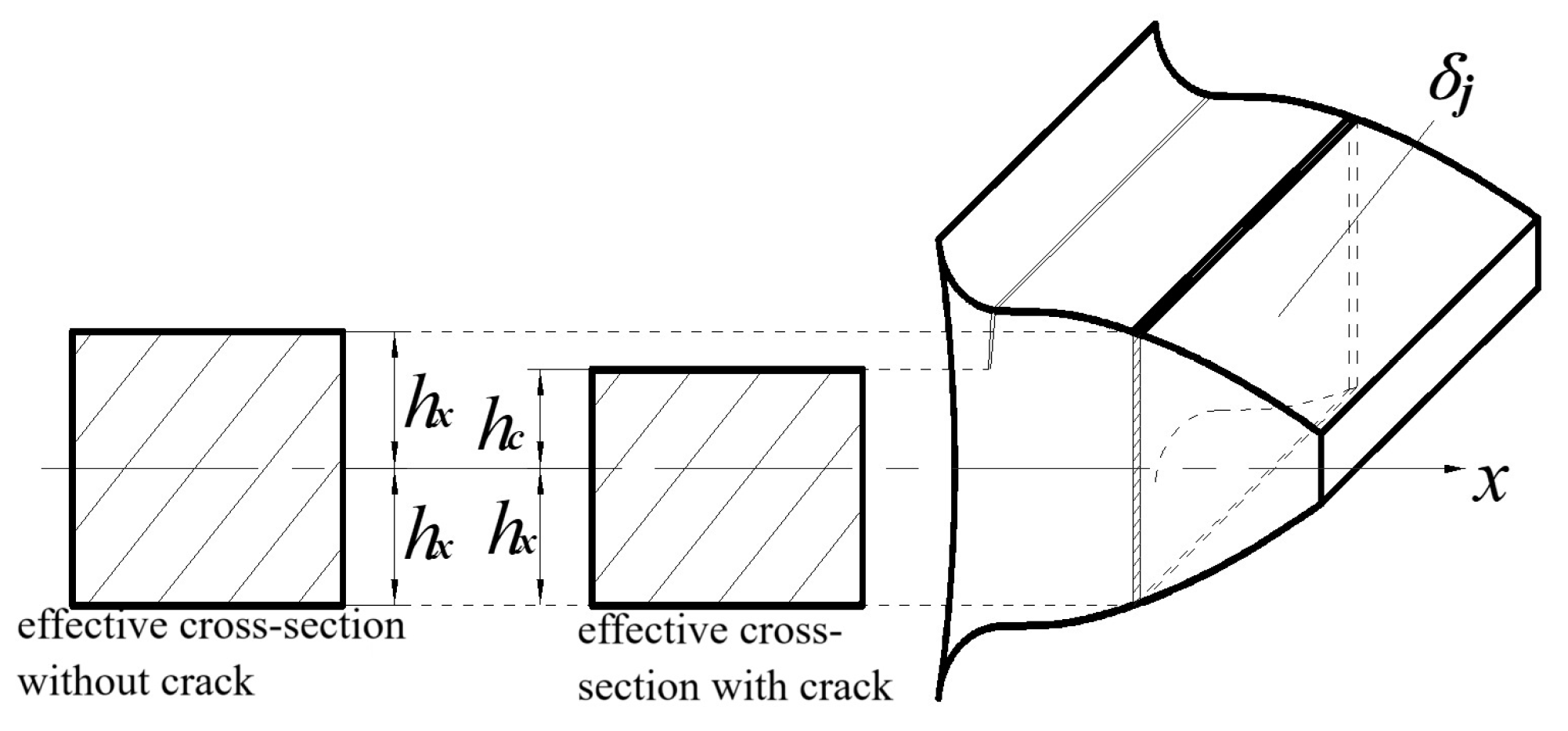
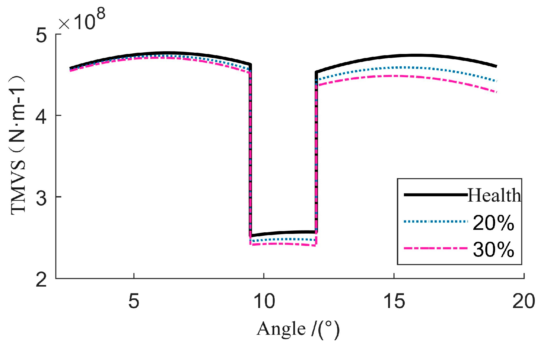
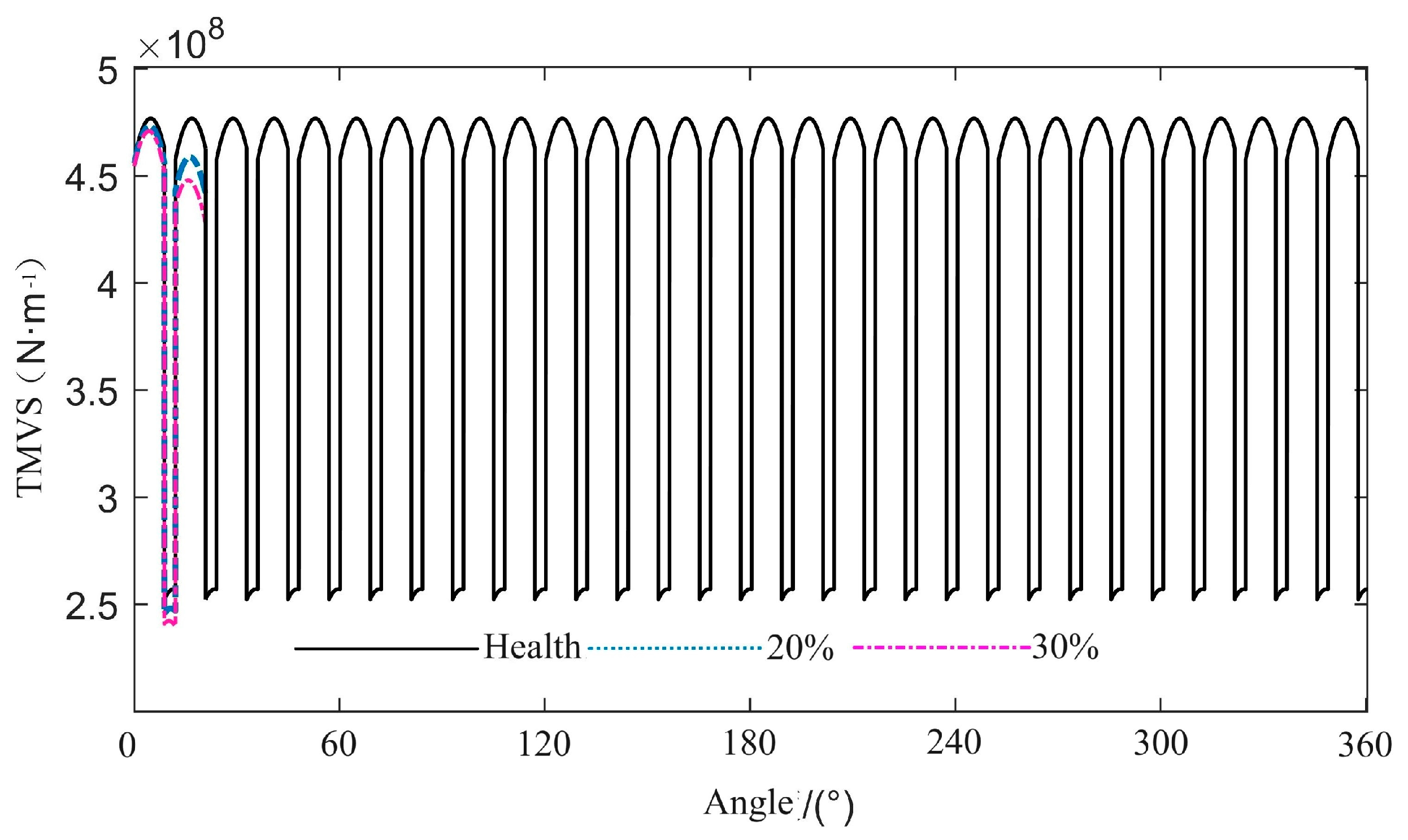
2.5. TVMS Considering Tooth Crack

Tooth root cracks represent a common internal fault in gears and pose a significant risk to the integrity of GTS. The accurate modeling of these cracks is crucial for understanding their impact on the dynamic behaviors of system. In this study, an analytical approach is employed to determine the meshing stiffness of gears that are influenced by the presence of cracks. By altering stiffness calculation methodologies [28], the meshing stiffness of gears affected by cracks can be ascertained, facilitating analysis of their electromechanical characteristics. The calculation method for the time-varying meshing stiffness of gears without considering tooth root cracks is shown in Appendix B.
During the meshing process, the stress experienced by gears closely resembles that of a cantilever beam. This similarity allows for the application of the 30° tangent method to effectively identify the tooth root as the critical section. This method entails drawing two lines at 30° angles to the tooth’s center of symmetry, both tangent to the fillet curve at the root. The intersection points of these lines, known as the tangent points, are then used to create a section parallel to the gear axis. As illustrated in Figure 6, this section is designated as the critical section at the tooth root.
After a crack appears in a gear, the calculation of bending, shear, and axial compressive deformation of the gear tooth section under the influence of meshing force is affected. As shown in Figure 7, the effective cross-section resisting bending along the tooth thickness direction for a gear with a root crack is hc + hx, whereas for a normal gear without cracks, the effective cross-section is hx + hx. If the crack depth is q, the effective height on the side with the crack in the tooth thickness direction is given by
h c = y t q sin θ
The moment of inertia Ix and the cross-sectional area Ax of the selected calculation element δj at a distance x from the tooth root are as follows, where Ix and Ax correspond to the moment of inertia and cross-sectional area in Equation (A5), respectively.
I x = 1 12 b h x + h c             y t h c 1 12 b h x + h x             y t h c
A x = b h x + h c             y t h c b h x + h x             y t h c
This ratio is utilized to quantify the severity of the crack and its impact on the gear’s meshing stiffness. In this study, the tooth root crack is assumed to be located on the pinion, which serves as the driving gear in the gear pair. This selection is based on the observation that cracks on the pinion tend to have a more significant influence on the system’s dynamic response due to its higher rotational speed and greater load-bearing capacity. Figure 8 presents the computed meshing stiffness results for various depths of tooth root cracks, compared with those of normal gears. The gear parameters are outlined in Table 1. In Figure 8, the percentage of tooth root crack depth is defined as the ratio of the crack depth (q) to the tooth thickness (hx).
When a gear contains a single crack, the cracked tooth engages once during a full rotation. In accordance with the principle of involute gear meshing, the meshing process of the cracked tooth can be described as follows:
  • Double-tooth engagement: Initially, the cracked tooth engages in double-tooth engagement, maintaining contact with the preceding gear tooth.
  • Transition to single-tooth engagement: As the engagement progresses, the cracked tooth transitions into a single-tooth engagement state.
  • Reversion to double-tooth engagement: Upon the engagement of the subsequent gear tooth, the cracked tooth reverts to a double-tooth engagement configuration.
The cracked tooth is observed to transition from double-tooth to single-tooth engagement and then revert to double-tooth engagement within a single meshing cycle. The variation in TVMS throughout a complete shaft rotation is depicted in Figure 9.

3. Verification of the Proposed Model

To address the electromechanical coupling dynamics of MGS, a comprehensive dynamic model was introduced. To ascertain the accuracy and efficacy of this innovative model, experimental validation is conducted using a specialized test platform.

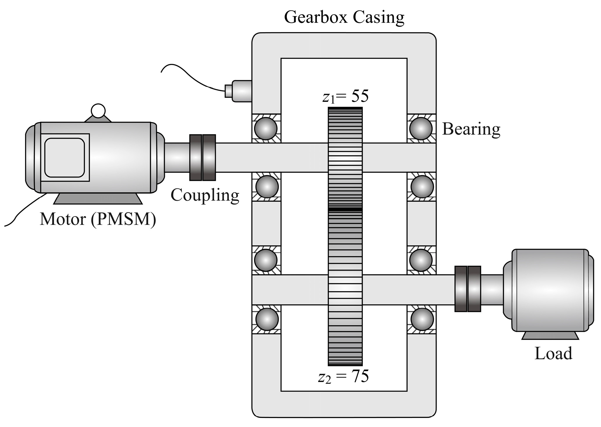
3.1. Introduction of Experimental Platform

The experimental test setup is illustrated in Figure 10, which includes a gearbox, a variable frequency AC motor, a magnetic powder brake, an acceleration sensor, a data acquisition system, controllers, and various auxiliary elements. Operating at a rated power of 1.5 kW, the motor’s speed is adjustable from 0 to 1500 rpm. The magnetic powder brake, attached to the output shaft, facilitates the application of load, with the brake torque controllable from 0 to 10 N·m via the brake controller. The gearbox houses two shafts supported by four rolling bearings. Additional gear parameters are detailed in Table 1 and Table 2. The acceleration sensor is installed on the exterior of the gearbox, close to the bearing supports of the gear shafts, to collect vibration information at the bearings. The collected data are then compared with the simulation results of the MGS model, with the comparison variable being the bearing vibration response yb.

3.2. Model Verification

The effectiveness of the electromechanical coupling dynamic model for the MGS is validated through experiments conducted on a specialized test platform. Figure 11 and Figure 12 illustrate the comparative results under various conditions. The experimental data reveal the vertical acceleration vibration signal of the gearbox input shaft, while the simulation results represent the lateral acceleration of the gear center. Both time-domain signals and their corresponding frequency spectra are presented for detailed analysis.
The vibration acceleration signal of the gearbox, both in its healthy state and with a crack present, exhibits harmonic patterns alongside chaotic behavior. This complexity complicates the identification of fluctuation periods. Analysis of the frequency spectrum indicates the presence of three primary frequencies: rotational frequency (fr), meshing frequency (fm), and twice of meshing frequency (2fm), accompanied by dense sidebands. The comparison between simulation and experimental results highlights several key findings:
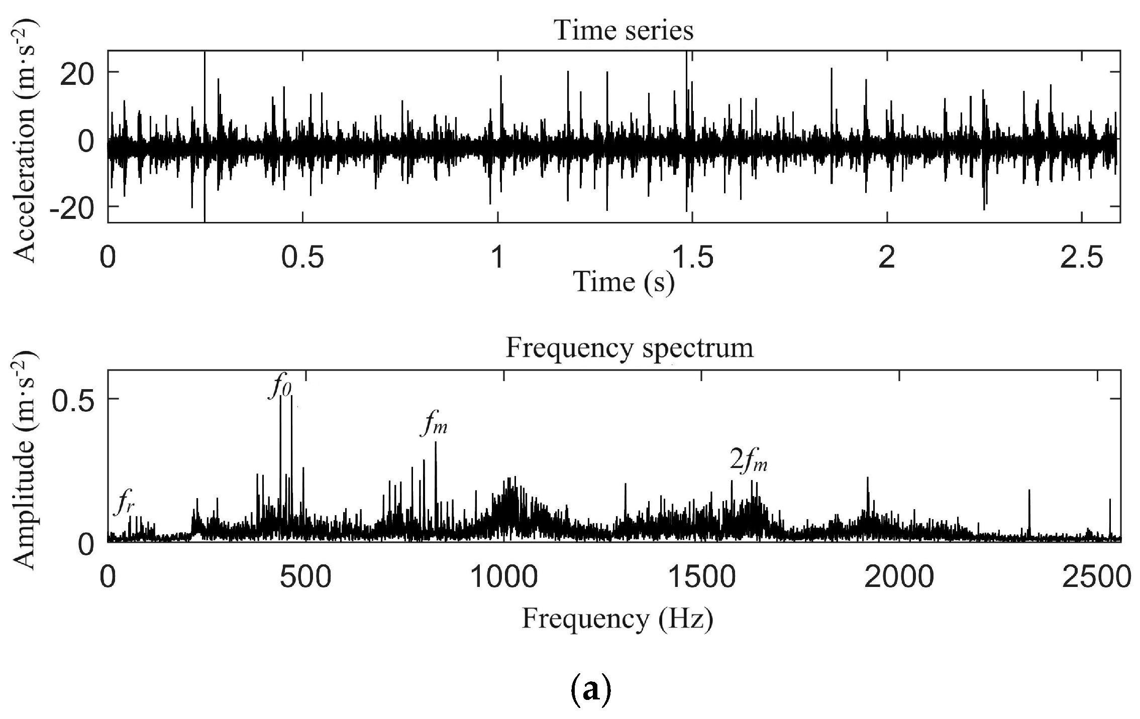
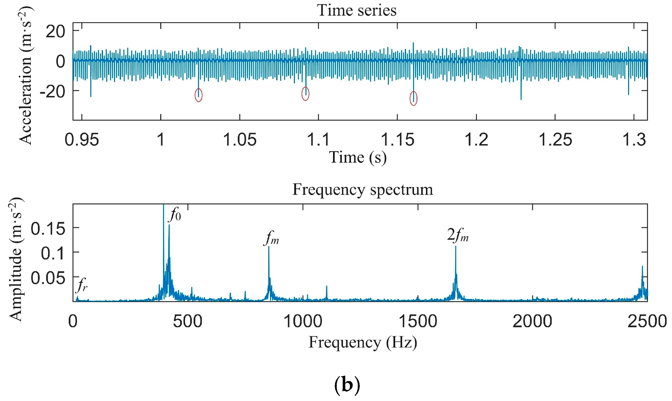
  • Similarity in Time-Domain Signal: Both the simulation and experimental results display harmonic vibration patterns, suggesting that the simulation model accurately represents the system dynamics.
  • Difference in Fluctuation Amplitude: The experimental results exhibit larger vibration acceleration amplitudes compared to the simulation, likely due to the complexities inherent in the real-world experimental setup.
  • Consistency in Frequency Components: Both the simulation and experimental results identify the same primary frequency components, including the rotational frequency (fr), meshing frequency (fm), and twice of meshing frequency (2fm).
  • Comparison of Sideband Components: The simulation results display fewer sidebands around the primary frequency components than the experimental results, highlighting the idealized conditions of the simulation model.
  • Simulation of Tooth Root Cracks: In a healthy system, the rotational frequency components are minimal. However, with a tooth root crack, the time-domain graph exhibits periodic harmonics, and the rotational frequency becomes more pronounced in the frequency spectrum.

4. Electromechanical Coupling Dynamics Simulation

This section delves into the effects of tooth root cracks, a prevalent fault in gear transmissions, on the dynamic characteristics of MGS. Gear mesh stiffness excitation data resulting from tooth root cracks are integrated into a multi-coupled dynamic model. The simulation analysis explores the impact of varying crack depths on system dynamics.

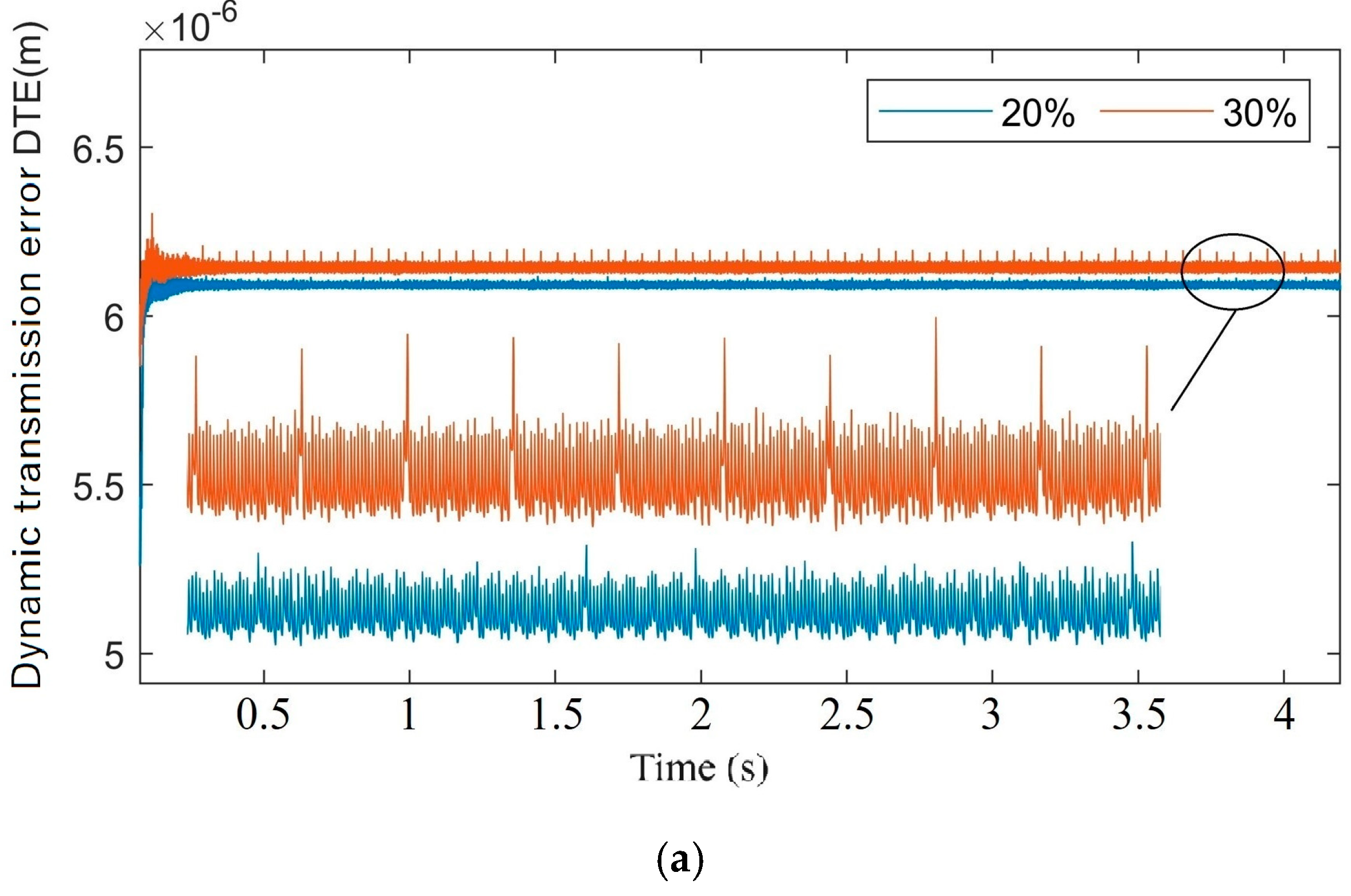
4.1. The Effect of Cracks on Gear Dynamics

The simulation results of gear root displacement along the mesh line for varying crack depths are illustrated in Figure 13. It is observed that gear vibrations are intensified with increasing crack depth, and the frequency spectrum exhibits sidebands associated with the rotational frequency near the natural frequency. These findings corroborate the experimental results detailed in Section 3.2. It is noted that tooth root cracks significantly influence the vibration characteristics of the GTS, altering both the mean value and amplitude of vibrations. A detailed analysis reveals that deeper cracks result in more pronounced impact characteristics and more distinct fault frequencies within gear vibrations.
The dynamic simulation results of gear dynamic transmission error (DTE) with varying tooth root crack depths are depicted in Figure 14. The presence of the tooth root crack is observed to introduce noticeable periodic impact vibrations into the DTE. Additionally, the frequency spectrum indicates multiple frequency modulations caused by meshing force fluctuations during transmission, which align with the observed actual conditions.
The depth of the tooth root crack is observed to directly influence both the gear center vibrations and the DTE of GTS. An increase in crack depth results in elevated mean values and amplitudes of gear center vibrations and DTE. Detailed analysis of the DTE reveals that greater crack depth intensifies gear meshing impacts. The frequency response also indicates that deeper cracks introduce more fault frequencies. These results demonstrate the effectiveness of the proposed multiple coupled dynamic model of the MGS in studying the dynamic impact of external excitations and internal excitation disturbances on mechanical vibrations. The model is shown to accurately simulate the dynamic characteristics of the MGS under fault conditions.

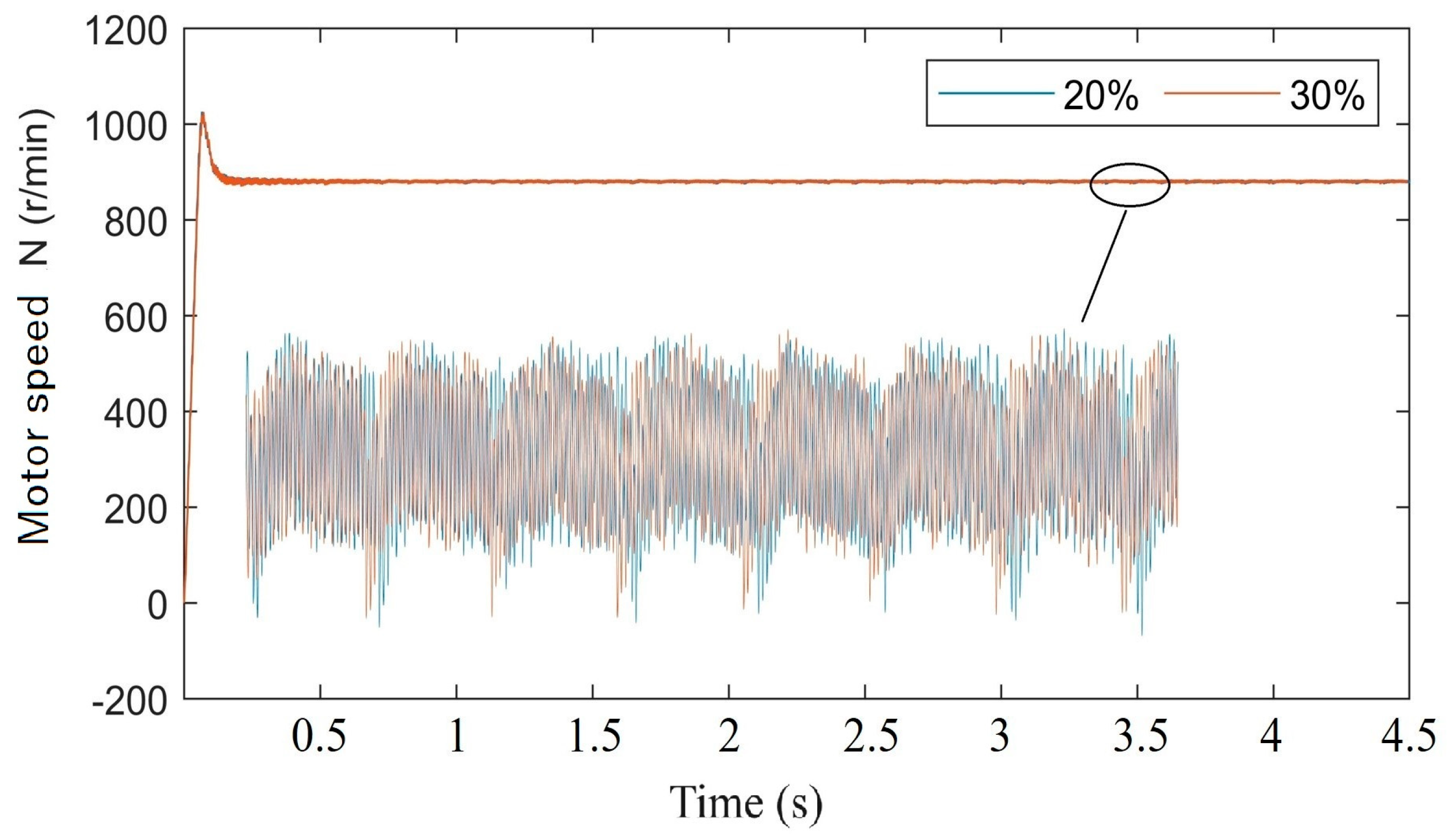
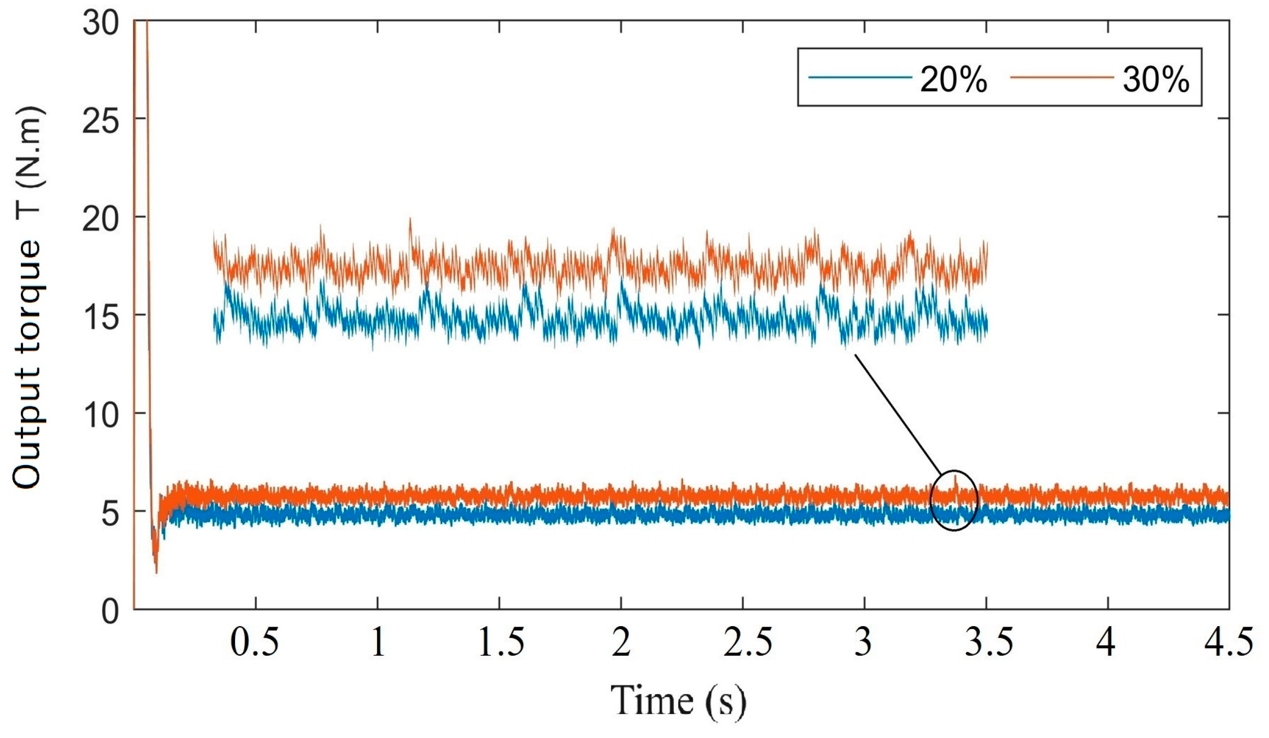
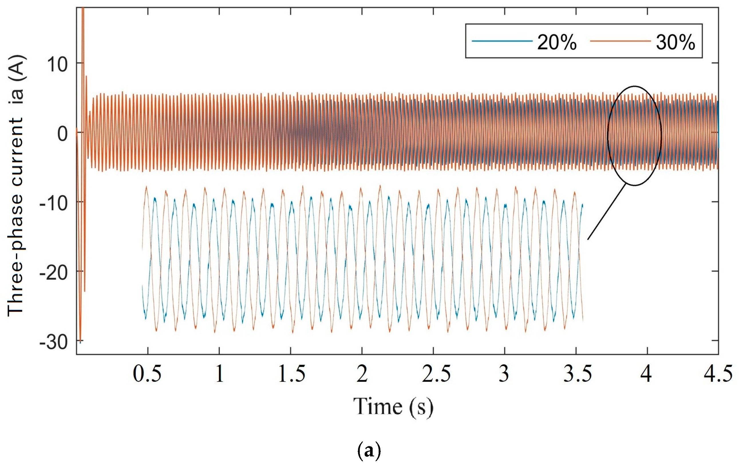
4.2. The Effect of Cracks on Motor Dynamics

The alterations in mechanical vibration characteristics induced by tooth root cracks were analyzed in the aforementioned study. Subsequently, the effects of these cracks on the motor dynamic response are explored. Figure 15 illustrates the actual output speed of the motor, as predicted by the proposed model. It is observed that the presence of tooth root cracks results in fluctuations in the motor output speed, with frequencies corresponding to the fluctuations observed in the DTE response. This indicates that the meshing impacts of tooth root cracks have an indirect influence on motor performance
Figure 16 depicts the actual output torque response of the motor for varying depths of tooth root cracks. The torque fluctuations are observed to mirror those in speed, both exhibiting impact effects. These observations suggest that tooth root crack faults induce unstable motion states within the GTS, such as meshing impacts and abnormal vibrations, which in turn affect the motor output characteristics. With the evolution of electric drive products towards more integrated and compact system structures, the significance of these impacts is expected to increase.
As shown in Figure 17, the dynamic response of motor current varies with tooth root crack depth. The amplitude of motor current is observed to be increased due to the presence of tooth root cracks. Compared to Figure 11, the current spectrum with cracks shows two frequency clusters around the main frequency. The frequency difference between these clusters equals the rotational frequency. This phenomenon is recognized as a new method for diagnosing mechanical faults in electric drive systems. Monitoring motor current, abnormal operations can be effectively detected, especially in situations where gearbox signal monitoring proves to be challenging.
These results demonstrate that internal excitations from tooth root cracks exert a direct impact on the dynamic characteristics of the GTS within MGS and also have an indirect effect on the dynamic properties of motor responses. With the evolution of electric drive products towards more compact and integrated structures, it is expected that these effects will be significantly amplified.

5. Conclusions

The challenges in vibration analysis and fault diagnosis of integrated electromechanical MGS under fault conditions are addressed in this paper. A novel electromechanical coupled dynamic model is introduced, which is designed for the design and optimization of MGS. The model is characterized by significant flexibility in parameter adjustments, making it suitable for various engineering scenarios. Then, the influence of various tooth root crack depths on the dynamic behavior of MGS is simulated by the model. One key finding is that the dynamic behaviors of both GTS and motor within MGS are affected by tooth root cracks. This capability offers a new approach for system fault diagnosis by allowing for the identification and analysis of fault signatures associated with different crack conditions. Although the accuracy of the vibration response of MGS has been experimentally verified in this study, further experimental validation of the motor response is still pending and will be addressed in future work.

Author Contributions

Z.Y., T.L., Q.C. and H.R. wrote the main manuscript text and Z.Y. prepared all figures. All authors have read and agreed to the published version of the manuscript.

Funding

The work is supported by the Key Technologies Research and Development Program of China (2023YFB3406601), National Natural Science Foundation of China (52275055), and Major Science and Technology Plan Projects of Xiamen (3502Z20231013).

Data Availability Statement

Data are contained within the article.

Conflicts of Interest

The authors declared no potential conflicts of interest with respect to the research, authorship, and/or publication of this article.

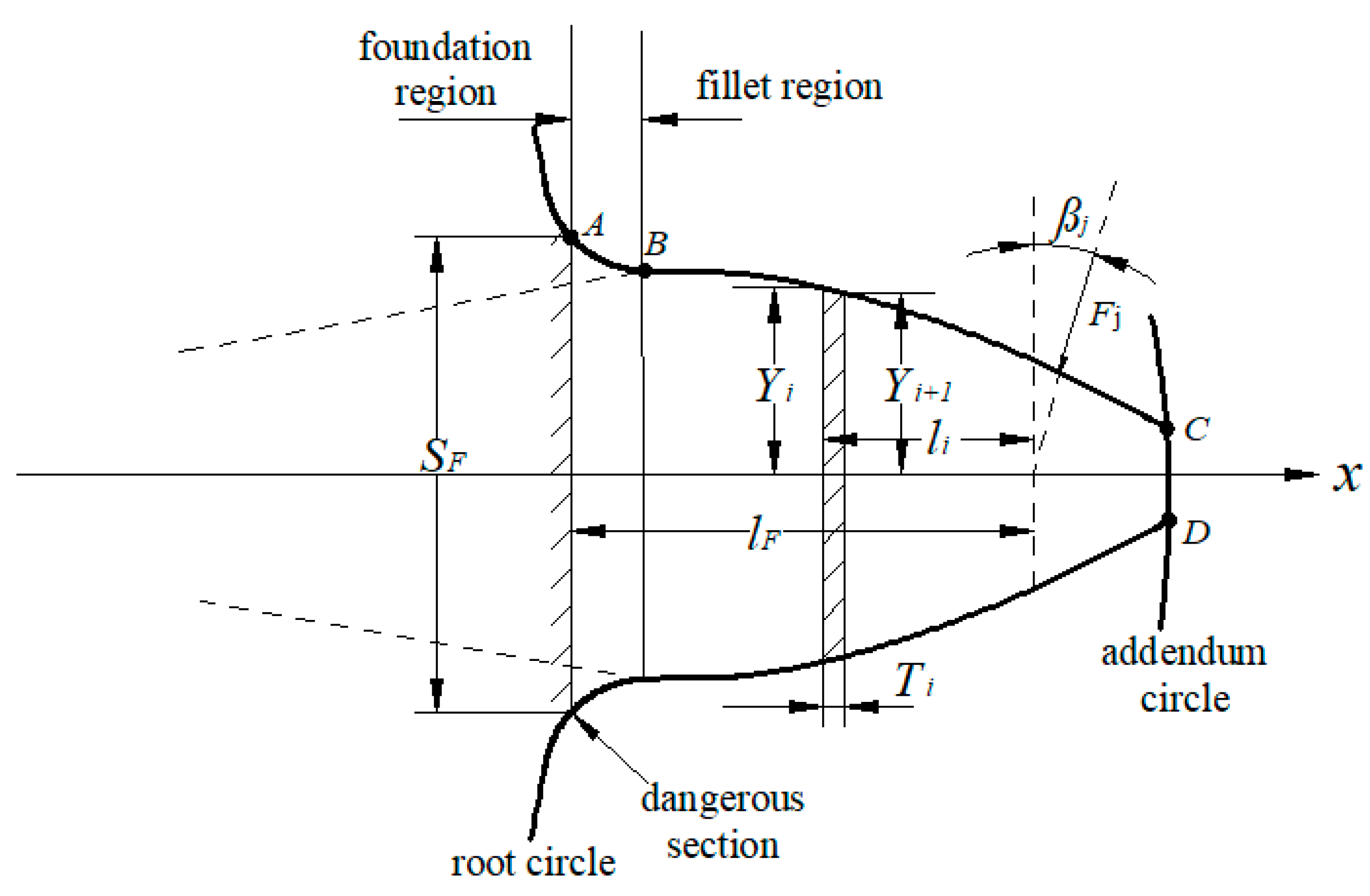
Appendix A. Calculation of TVMS

As shown in Figure A1, a gear tooth can be modeled as a nonuniform cantilever beam [28,32,40]. Its deformation depends on four components:
  • Local Deformation (δL): Resulting from contact between the teeth.
δ L = 4 F j π B ( 1 ν 1 2 E 1 + 1 ν 2 2 E 2 )
where νi denotes Poisson’s ratio, Ei is the modulus of elasticity, Fj represents the load, and B is the tooth width.
2.
Gear Body Contribution (δFB): The effect of the gear body on tooth deflection.
δ F B = F j cos 2 β j E e B [ L * ( l F S F ) 2 + M * ( l F S F ) 2 + P * ( 1 + Q * tan 2 β j ) ]
where L*, M*, P*, and Q* are functions of h and θf, h is ratio of root radius to gear bore, θf is related to gear parameters.
3.
Fillet Deflection (δFF): In the direction of the applied tooth load.
δ F F = F j i = 1 n cos 2 β j E e [ ( T A B ) i 3 3 + ( T A B ) i 2 + ( T A B ) i ( l A B ) i ( I ¯ A B ) i + 2.4 ( 1 + ν ) + tan 2 β j ( A ¯ A B ) i ] cos β j sin β j E e ( ( ( T A B ) i 2 ( Y ¯ A B ) i 2 + ( T A B ) i ( Y ¯ A B ) i ( l A B ) i ) ( I ¯ A B ) i ) + ( T A B ) i sin 2 β j ( A ¯ A B ) i E e
4.
Basic Deflection (δB): Includes bending, shearing, and axial deformation of the tooth as a beam.
δ B = F j cos 2 β j E e i = 1 n T i [ T i 2 3 + T i l i + l i 2 I ¯ i tan β j T i 2 Y ¯ i 2 + Y i l i I ¯ i + 2.4 ( 1 + ν ) + tan 2 β j A ¯ i ]
Here, li and Ti are as depicted in Figure A1. For each segment i, the height Y ¯ i , cross-sectional area A ¯ i , and area moment of inertia I ¯ i are calculated as the average values at both faces, using the following equations:
1 Y i ¯ = ( 1 Y i + 1 Y i + 1 ) / 2 1 A i ¯ = ( 1 A i + 1 A i + 1 ) / 2 = 2 × B × Y ¯ i 1 I ¯ i = ( 1 I i + 1 I i + 1 ) / 2 = B × ( Y i 3 + Y i + 1 3 ) / 3
where subscripts i and i + 1 represent the corresponding part of each side of segment i.
Figure A1. Geometry and segment model of the spur gear.
Machines 12 00918 g0a1
Hence, the deformation of gear teeth at a given moment can be expressed as
δ   =   ( δ F F + δ F B + δ B ) p + ( δ F F + δ F B + δ B ) g + δ L
where the subscripts p and g denote the deformations of the pinion and gear, respectively. The corresponding meshing stiffness at this moment is
k ( t ) = F j δ

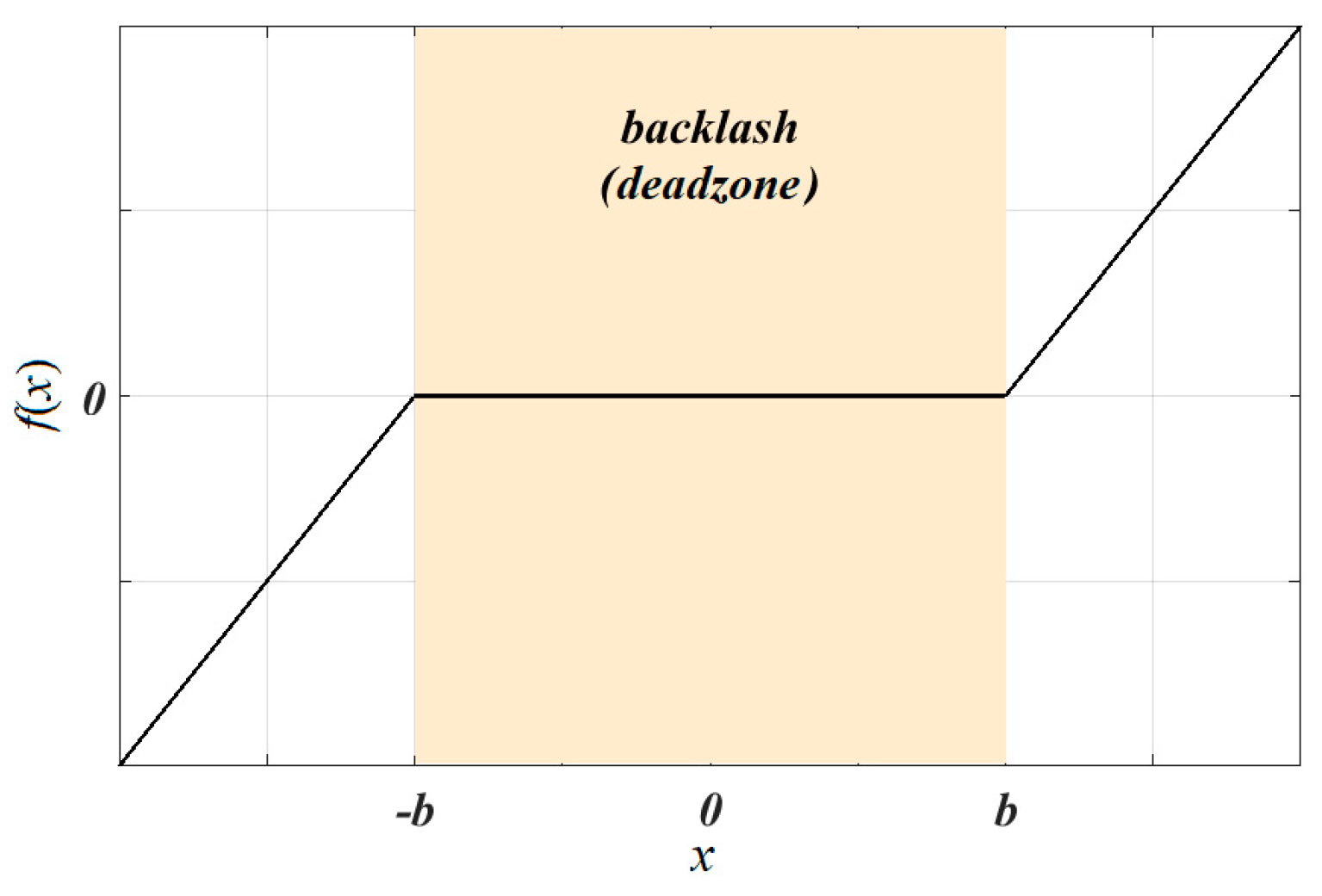
Appendix B. Calculation of Other Nonlinear Parameters in GTS

f(x) represents a discontinuous function of the gear along the direction of the mesh line, and its curve is shown in Figure A2, hence f(x) can be expressed as
f ( x ) = x b     x > b 0               b x b x + b     x < b
where b is the half value of the backlash, a dead zone to allow tooth separations.
Figure A2. Graphical visualization of the gear backlash characteristics.
Machines 12 00918 g0a2
Figure A3 shows the beginning of mesh cycle, pair1 (defined as the tooth pair rolling along line AC) comes into mesh at point A, and pair2 (defined as the tooth pair rolling along line CD) is contact at point C, which is the beginning of the double-tooth engagement. As the gear pair rolls, pair2 leaves contact at point D, which is the beginning of single-tooth engagement, and pair1 approaches at the point B when mesh time t is equal to tb. Finally, pair1 goes through point C when time t is equal to tc, and one mesh cycle is completed. At the same time, pair1 convert to pair2 and new pair1 of teeth come into mesh at point A.
Figure A3. A schematic diagram of the gear teeth mesh for involute spur gear pair.
Machines 12 00918 g0a3
Since the gear pair alternates between single and double tooth engagement, and the load on each tooth pair varies with the meshing position, the meshing forces assigned to each tooth are as follows:
F n p 1 = L d 1 ( t ) F n ,   F n g 1 = F n p 1 ,   F n p 2 = L d 2 ( t ) F n ,   F n g 2 = F n p 2
where Ld1(t) and Ld2(t) represent the time-varying sharing ratios [40]. In Equations (23) and (24), the frictions experienced by the pinion and gear are denoted by Ffi (i = p, g), respectively.
F f p 1 = λ ( t ) μ 1 ( t ) F n p 1 ,   F f g 1 = F f p 1 ,   F f p 2 = μ 2 ( t ) F n p 2 ,   F f g 2 = F f p 2
Here, μi(t) is a time-varying friction coefficient discussed below, and λ(t) is the direction coefficient of the friction forces as follows:
λ ( t ) = sgn [ t P mod ( t , t c ) ] s g n ( x ) = 1           i f x > 0 s g n ( x ) = 1         i f x 0 mod ( x , y ) = x y × floor ( x / y ) ,         if   y 0
in which floor(x) is a downward rounding function, and tP is a time spot when gear pair is meshing at pitch point. Let ωp be the angular velocity of pinion, rbp base circle radius of pinion, and Pb base pitch; then, one obtains
t c = P b ω p r b p ,   t b t c = L A B P b ,   t p t c = L A P P b
When considering torsional dynamics, it is essential to determine the moment arms associated with friction forces. Additionally, it should be noted that the moment arms of tooth pair 1 and pair 2 during double-teeth meshing are not identical. Let spi and sgi (i = 1, 2) represent the moment arms on the pinion and gear, respectively, for the friction forces acting on the i-th meshing tooth pair.
s p 1 = L N 1 A + mod ( ω p r b p t , P b ) ,   s p 2 = L N 1 A + P b + mod ( ω p r b p t , P b ) ,   s g 1 = L N 1 C + P b mod ( ω g r b g t , P b ) ,   s g 2 = L N 1 C mod ( ω g r b g t , P b )
where LN1i (i = A, C) is the distance from N1 to i which can be seen from Figure A3. Based on this, the following equations can be readily derived: Ffp = Ffp1 + Ffp2 and Ffg = Ffg1 + Ffg2.

References

  1. Mohammed, O.D.; Rantatalo, M. Gear fault models and dynamics-based modelling for gear fault detection—A review. Eng. Fail. Anal. 2020, 117, 104798. [Google Scholar] [CrossRef]
  2. Cooley, C.G.; Parker, R.G. A review of planetary and epicyclic gear dynamics and vibrations research. Appl. Mech. Rev. 2014, 66, 040804. [Google Scholar] [CrossRef]
  3. Husain, I.; Ozpineci, B.; Islam, S.; Gurpinar, E.; Su, G.J.; Yu, W.; Chowdhury, S.; Xue, L.; Rahman, D.; Sahu, R. Electric drive technology trends, challenges, and opportunities for future electric vehicles. Proc. IEEE 2021, 109, 1039–1059. [Google Scholar] [CrossRef]
  4. Zhu, L.Y.; Yang, W.J.; Gou, X.F.; Li, Z.F. Dynamic characteristics of spur gear pair considering meshing impact and multi-state meshing. Meccanica 2023, 58, 619–642. [Google Scholar] [CrossRef]
  5. Szolc, T.; Konowrocki, R.; Michajłow, M.; Pręgowska, A. An investigation of the dynamic electromechanical coupling effects in machine drive systems driven by asynchronous motors. Mech. Syst. Signal Process. 2014, 49, 118–134. [Google Scholar] [CrossRef]
  6. Liu, C.; Wang, L.; Zhang, T.; Chen, X.; Ge, S. Electromechanical dynamic analysis for powertrain of off-grid switched-reluctance wind turbine hydrogen production system. Renew. Energy 2023, 208, 214–228. [Google Scholar] [CrossRef]
  7. Chen, R.; Qin, D.; Liu, C. Dynamic modelling and dynamic characteristics of wind turbine transmission gearbox-generator system electromechanical-rigid-flexible coupling. Alex. Eng. J. 2023, 65, 307–325. [Google Scholar] [CrossRef]
  8. Jiang, S.; Li, W.; Wang, Y.; Yang, X.; Xu, S. Study on electromechanical coupling torsional resonance characteristics of gear system driven by PMSM: A case on shearer semi-direct drive cutting transmission system. Nonlinear Dyn. 2021, 104, 1205–1225. [Google Scholar] [CrossRef]
  9. Kumar, V.; Rai, A.; Mukherjee, S.; Sarangi, S.A. Lagrangian approach for the electromechanical model of single-stage spur gear with tooth root cracks. Eng. Fail. Anal. 2021, 129, 105662. [Google Scholar] [CrossRef]
  10. Ryali, L.; Talbot, D. A dynamic gear load distribution model for epicyclic gear sets with a structurally compliant planet carrier. Mech. Mach. Theory 2023, 181, 105225. [Google Scholar] [CrossRef]
  11. Zghal, B.; Graja, O.; Dziedziech, K.; Chaari, F.; Jablonski, A.; Barszcz, T.; Haddar, M. A new modeling of planetary gear set to predict modulation phenomenon. Mech. Syst. Signal Process. 2019, 127, 234–261. [Google Scholar] [CrossRef]
  12. Hao, L.; Li, W.; Zhang, X. Impact of Gear Modification on Gear Dynamic Characteristics. J. Fail. Anal. Prev. 2023, 23, 853–864. [Google Scholar] [CrossRef]
  13. Zhang, C.; Wei, J.; Hou, S.; Zhang, J. Scaling law of gear transmission system obtained from dynamic equation and finite element method. Mech. Mach. Theory 2021, 159, 104285. [Google Scholar] [CrossRef]
  14. Zhou, C.; Jiang, X.; Su, J.; Liu, Y.; Hou, S. Injection lubrication for high-speed helical gears using the overset mesh method and experimental verification. Tribol. Int. 2022, 173, 107642. [Google Scholar] [CrossRef]
  15. Jedliński, Ł. Influence of gear eccentricity with non-parallel axis on the dynamic behaviour of a gear unit using a gear slice model with 26 degrees of freedom. Adv. Sci. Technol. Res. J. 2024, 18, 88–102. [Google Scholar] [CrossRef]
  16. Bartelmus, W. Gearbox dynamic multi-body modelling for condition monitoring under the case of varying operating condition. J. Coupled Syst. Multiscale Dyn. 2014, 2, 224–237. [Google Scholar] [CrossRef]
  17. Sakaridis, E.; Spitas, V.; Spitas, C. Non-linear modeling of gear drive dynamics incorporating intermittent tooth contact analysis and tooth eigenvibrations. Mech. Mach. Theory 2019, 136, 307–333. [Google Scholar] [CrossRef]
  18. Gong, H.; Shu, R.; Xiong, Y.; Xie, Z.; Huang, J.; Tan, R.; Yin, Q.; Zou, Z. Dynamic response analysis of a motor–gear transmission system considering the rheological characteristics of magnetorheological fluid coupling. Nonlinear Dyn. 2023, 111, 13781–13806. [Google Scholar] [CrossRef]
  19. Fateh, F.; White, W.N.; Gruenbacher, D. Torsional vibrations mitigation in the drivetrain of DFIG-based grid-connected wind turbine. IEEE Trans. Ind. Appl. 2017, 53, 5760–5767. [Google Scholar] [CrossRef]
  20. Féki, N.; Clerc, G.; Velex, P. Gear and motor fault modeling and detection based on motor current analysis. Electr. Power Syst. Res. 2013, 95, 28–37. [Google Scholar] [CrossRef]
  21. Lu, W.; Zhang, Y. Research on the effect of tooth root defects on the motor-multistage gear transmission system. Mech. Based Des. Struct. Mach. 2024, 53, 1561–1583. [Google Scholar] [CrossRef]
  22. Ge, S.; Hou, S.; Zhang, Z.; Wang, H.; Li, W. Electromechanical coupling dynamics of dual-motor electric drive system of hybrid electric vehicles. Proc. Inst. Mech. Eng. Part D J. Automob. Eng. 2024, 09544070241230703. [Google Scholar] [CrossRef]
  23. Marzebali, M.H.; Kia, S.H.; Henao, H.; Capolino, G.A.; Faiz, J. Planetary gearbox torsional vibration effects on wound-rotor induction generator electrical signatures. IEEE Trans. Ind. Appl. 2016, 52, 4770–4780. [Google Scholar] [CrossRef]
  24. Kumar, S.; Kumar, V.; Chandan, P.U.; Sarangi, S. Electromechanical Modelling and Multi Faults Diagnosis of Straight Bevel Gear Pair with Experimental Validation. J. Vib. Eng. Technol. 2024, 12, 79–92. [Google Scholar] [CrossRef]
  25. Han, Q.; Jiang, Z.; Kong, Y.; Wang, T.; Chu, F. Motor current model for detecting localized defects in planet rolling bearings. IEEE Trans. Ind. Electron. 2022, 70, 9483–9494. [Google Scholar] [CrossRef]
  26. Ouyang, T.; Wang, G.; Cheng, L.; Wang, J.; Yang, R. Comprehensive diagnosis and analysis of spur gears with pitting-crack coupling faults. Mech. Mach. Theory 2022, 176, 104968. [Google Scholar] [CrossRef]
  27. Molaie, M.; Samani, F.S.; Zippo, A.; Iarriccio, G.; Pellicano, F. Spiral bevel gears: Bifurcation and chaos analyses of pure torsional system. Chaos Solit. Fractals 2023, 177, 114179. [Google Scholar] [CrossRef]
  28. Sang, M.; Huang, K.; Xiong, Y.; Han, G.; Cheng, Z. Dynamic modeling and vibration analysis of a cracked 3K-II planetary gear set for fault detection. Mech. Sci. 2021, 12, 847–861. [Google Scholar] [CrossRef]
  29. Chai, N.; Yang, M.; Ni, Q.; Xu, D. Gear fault diagnosis based on dual parameter optimized resonance-based sparse signal decomposition of motor current. IEEE Trans. Ind. Appl. 2018, 54, 3782–3792. [Google Scholar] [CrossRef]
  30. El Yousfi, B.; Soualhi, A.; Medjaher, K.; Guillet, F. Electromechanical modeling of a motor–gearbox system for local gear tooth faults detection. Mech. Syst. Signal Process. 2022, 166, 108435. [Google Scholar] [CrossRef]
  31. Sheng, L.; Sun, Q.; Li, W.; Ye, G. Research on gear crack fault diagnosis model based on permanent magnet motor current signal. ISA Trans. 2023, 135, 188–198. [Google Scholar] [CrossRef]
  32. Chen, Z.; Zhang, J.; Wang, K.; Liu, P. Nonlinear dynamic responses of locomotive excited by rail corrugation and gear time-varying mesh stiffness. Transport 2022, 37, 383–397. [Google Scholar] [CrossRef]
  33. Ottewill, J.R.; Ruszczyk, A.; Broda, D. Monitoring tooth profile faults in epicyclic gearboxes using synchronously averaged motor currents: Mathematical modeling and experimental validation. Mech. Syst. Signal Process. 2017, 84, 78–99. [Google Scholar] [CrossRef]
  34. Liu, X.; Hou, M. Dynamic Characteristic Analysis of Permanent Magnet Toroidal Motor. In Proceedings of the 2019 Chinese Control Conference (CCC), Guangzhou, China, 27–30 July 2019; pp. 7174–7179. [Google Scholar]
  35. Ullah, K.; Guzinski, J.; Mirza, A.F. Critical review on robust speed control techniques for permanent magnet synchronous motor (PMSM) speed regulation. Energies 2022, 15, 1235. [Google Scholar] [CrossRef]
  36. Parvez, M.; Elias, M.F.M.; Rahim, N.A.; Blaabjerg, F.; Abbott, D.; Al-Sarawi, S.F. Comparative study of discrete PI and PR controls for single-phase UPS inverter. IEEE Access 2020, 8, 45584–45595. [Google Scholar] [CrossRef]
  37. Kim, H.; Sikanen, E.; Nerg, J.; Sillanpää, T.; Sopanen, J.T. Unbalanced magnetic pull effects on rotor dynamics of a high-speed induction generator supported by active magnetic bearings—Analysis and experimental verification. IEEE Access 2020, 8, 212361–212370. [Google Scholar] [CrossRef]
  38. Tsuha, N.A.H.; Cavalca, K.L. Stiffness and damping of elastohydrodynamic line contact applied to cylindrical roller bearing dynamic model. J. Sound Vib. 2020, 481, 115444. [Google Scholar] [CrossRef]
  39. Salah, A.A.; Dorrell, D.G.; Guo, Y. A review of the monitoring and damping unbalanced magnetic pull in induction machines due to rotor eccentricity. IEEE Trans. Ind. Appl. 2019, 55, 2569–2580. [Google Scholar] [CrossRef]
  40. Yao, Z.; Wang, J.; Zhao, Y. Dynamic responses and control of geared transmission system based on multibody modeling methodology. J. Vib. Control 2023, 29, 543–561. [Google Scholar] [CrossRef]
Figure 1. The structure of the motor gear system.
Machines 12 00918 g001
Figure 2. Electromechanical coupling dynamic model of MGS.
Machines 12 00918 g002
Figure 3. Principal diagram of PMSM control.
Machines 12 00918 g003
Figure 4. Simplified model of the motor rotor.
Machines 12 00918 g004
Figure 5. Model of the GTS.
Machines 12 00918 g005
Figure 6. Critical section at the tooth root.
Machines 12 00918 g006
Figure 7. Effective cross-section at the crack location.
Machines 12 00918 g007
Figure 8. The comparison of meshing stiffness results.
Machines 12 00918 g008
Figure 9. The meshing stiffness for one rotation cycle.
Machines 12 00918 g009
Figure 10. Experimental test platform of GTS: 1. worktable; 2. tachometer; 3. speed controller; 4. PMSM; 5. gearbox; 6. vibration sensor; 7. magnetic powder brake; 8. brake control.
Machines 12 00918 g010
Figure 11. Comparison of lateral vibration acceleration without crack fault. (a) Experimental results of acceleration signal. (b) Simulation results of vibration acceleration.
Machines 12 00918 g011
Figure 12. Comparison of lateral vibration acceleration under fault of tooth root crack. (a) Experimental results of acceleration signal. (b) Simulation results of vibration acceleration.
Machines 12 00918 g012aMachines 12 00918 g012b
Figure 13. Dynamic response of displacement yp for different crack depths. (a) Time series response of yp. (b) Spectrum responses of yp.
Machines 12 00918 g013
Figure 14. Dynamic response of DTE for different crack depths. (a) Time series response of DTE. (b) Spectrum responses of DTE.
Machines 12 00918 g014aMachines 12 00918 g014b
Figure 15. The response of motor speed for different crack depth.
Machines 12 00918 g015
Figure 16. The response of motor torque for different crack depth.
Machines 12 00918 g016
Figure 17. The response of motor current FOR different crack depth. (a) Time series response of motor current. (b) Spectrum responses of motor current.
Machines 12 00918 g017aMachines 12 00918 g017b
Table 1. Parameters of the MGS.
MotorSymbol
Number of Pole Pairsnp3
Flux Linkage (Wb)ϕf0.175
Stator Resistance (Ω)R2.875
Moment of Inertia (kg·m2)J0.008
Stator Inductance (mH)Ld, Lq8.58.5
GearSymbolPinionGear
Number of teethz1, z25575
Mass (kg)mp, mg2.3283.937
Moment of inertia (kg∙m2)Jp, Jg0.01950.0614
Modules (mm)m2
Tooth width (mm)B20
Pressure angle (deg)α20
Pitch (mm)Pn5.9
Contact ratioε1.797
Addendum coefficient h a * 1
Tip clearance coefficientλ0.25
Elastic modulus (Pa)E210 G
Poisson’s ratioν0.28
Mass density (kg·m−3)ρ7800
Table 2. Parameters of the GTC.
ParameterSymbolInput ShaftOutput Shaft
Transverse stiffness (N/m)kpx, kgy3 × 1082 × 108
Transverse damping (N∙s/m)cgx, cgy1.1 × 1030.9 × 103
Torsional stiffness (N∙m/rad)kI, kO9 × 1067 × 106
Torsional damping (N∙m∙s/rad)cI, cO1711
Outer radius of the bearing (m)R1, R20.090.04
Inner radius of the bearing (m)r1, r20.050.02
Bearing clearance (mm)γ01, γ020.020.05
Number of bearing rollersN1, N21418
Contact stiffness of supports (N/m3/2)kb1, kb21.334 × 10101.056 × 1010
Disclaimer/Publisher’s Note: The statements, opinions and data contained in all publications are solely those of the individual author(s) and contributor(s) and not of MDPI and/or the editor(s). MDPI and/or the editor(s) disclaim responsibility for any injury to people or property resulting from any ideas, methods, instructions or products referred to in the content.

