
Assessment of Non-Linear Modeling of Ladle Furnace Transformer Using Finite Element Analysis


Abstract
1. Introduction
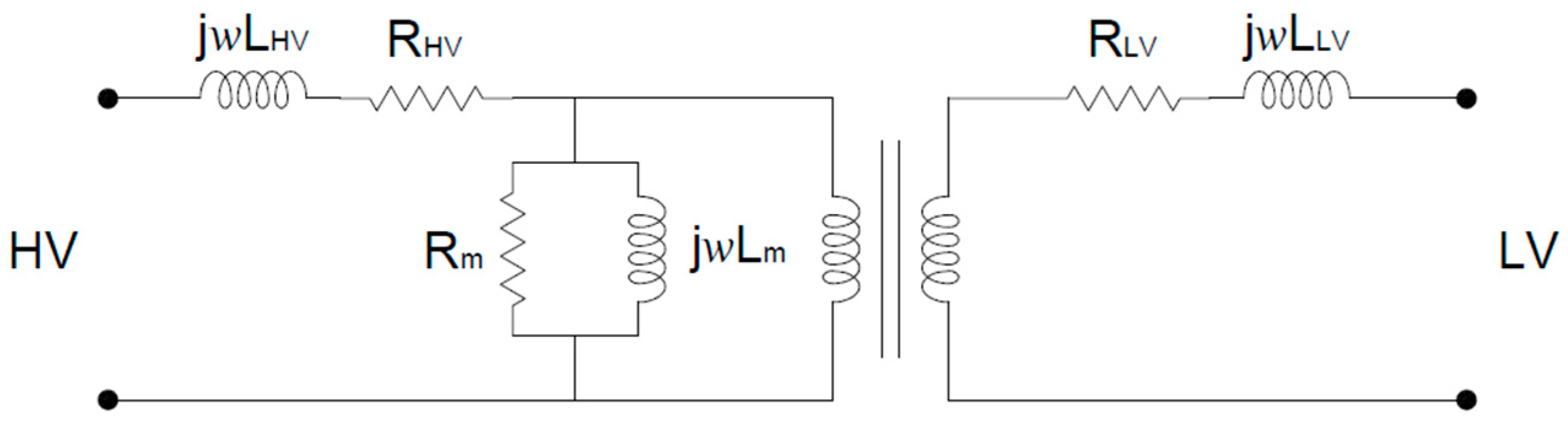
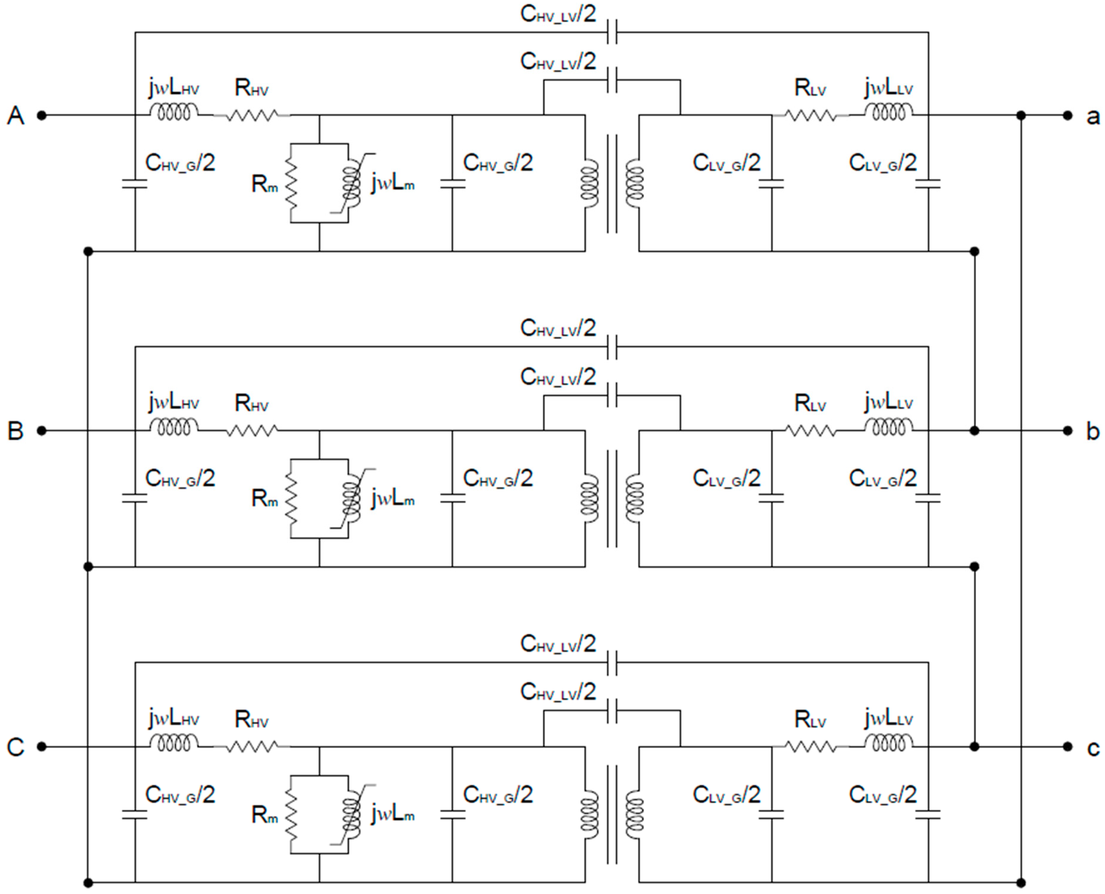
2. Proposed Model
3. Methodology for the Calculation of Parameters
3.1. Analytical Calculation of Impedances
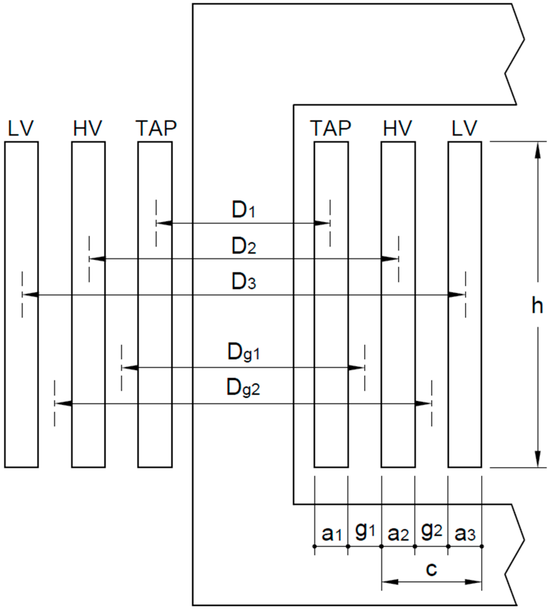
3.1.1. Leakage Impedances
3.1.2. Ohmic Resistance
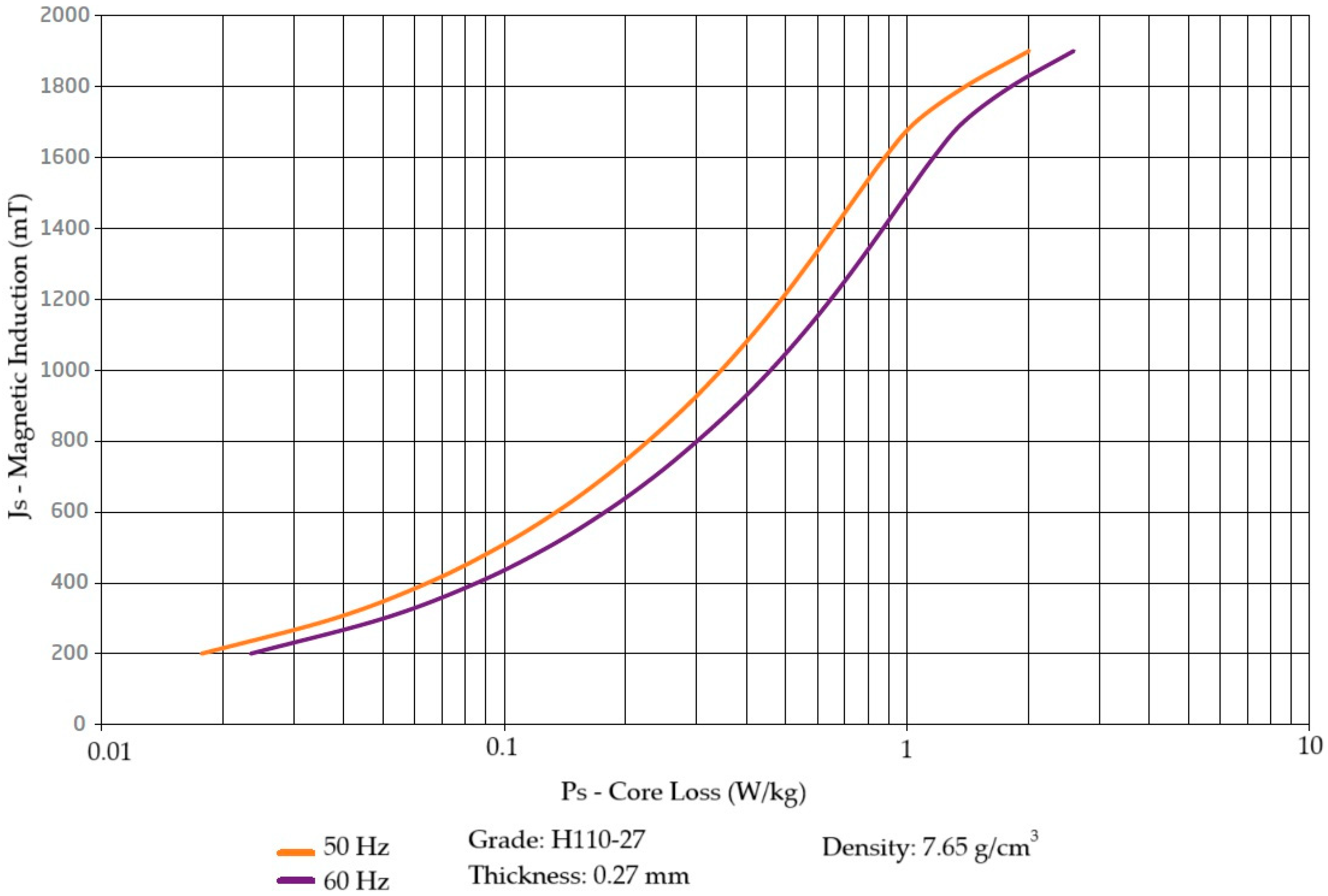
3.1.3. Iron Loss Resistance
3.1.4. Magnetizing Impedance
3.1.5. Capacitance
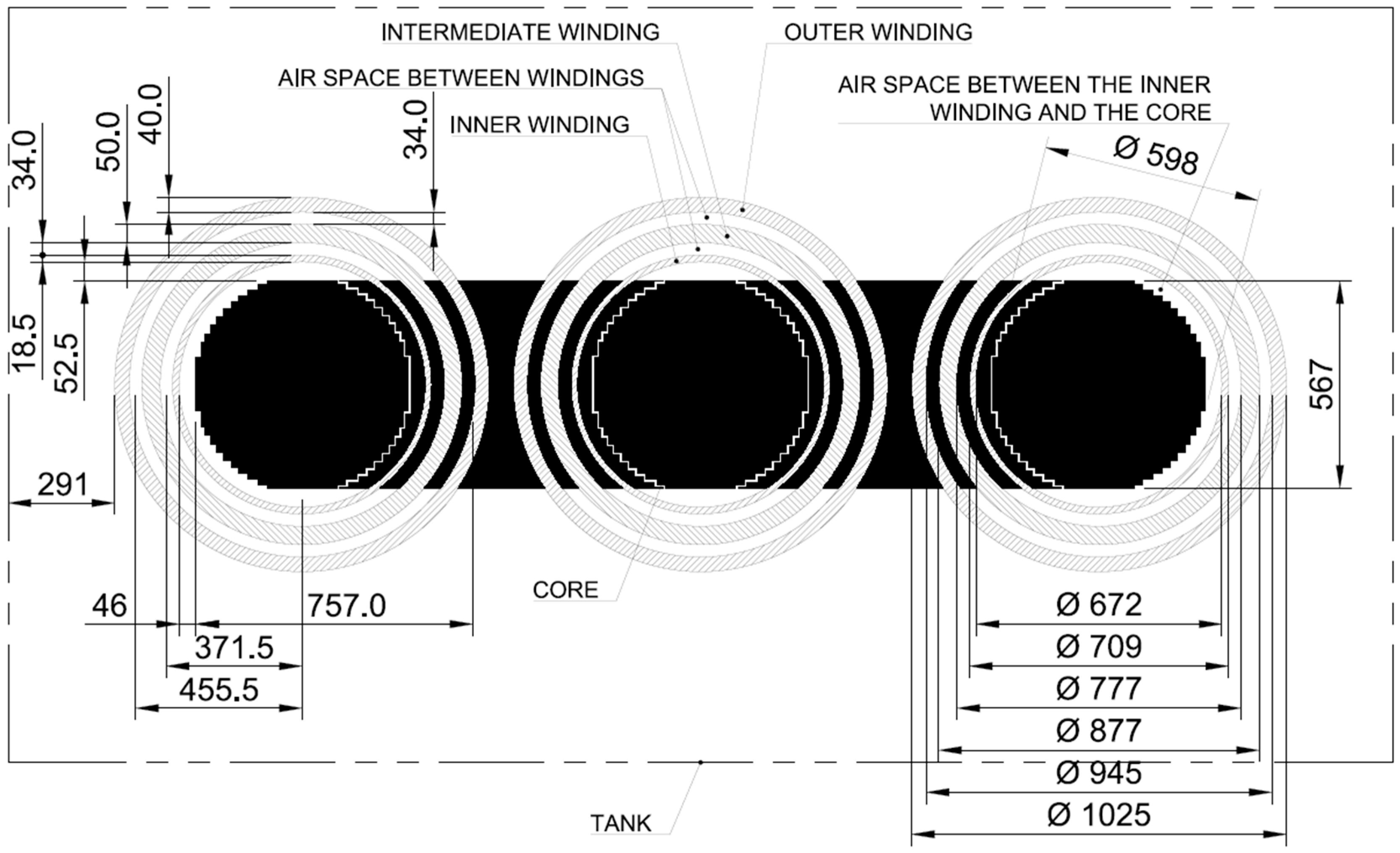
3.2. Transformer Modeling Using Finite Element Analysis
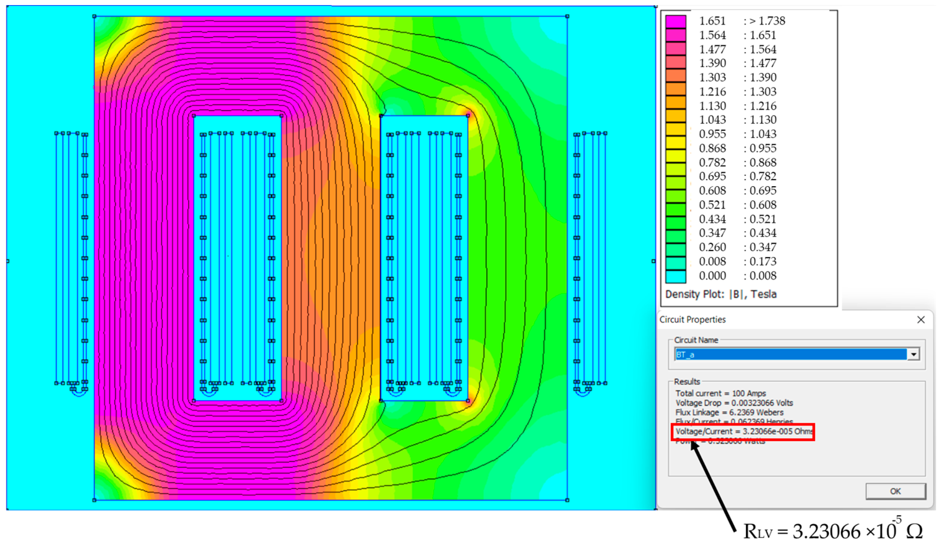
3.2.1. Leakage Impedances
3.2.2. Ohmic Resistance
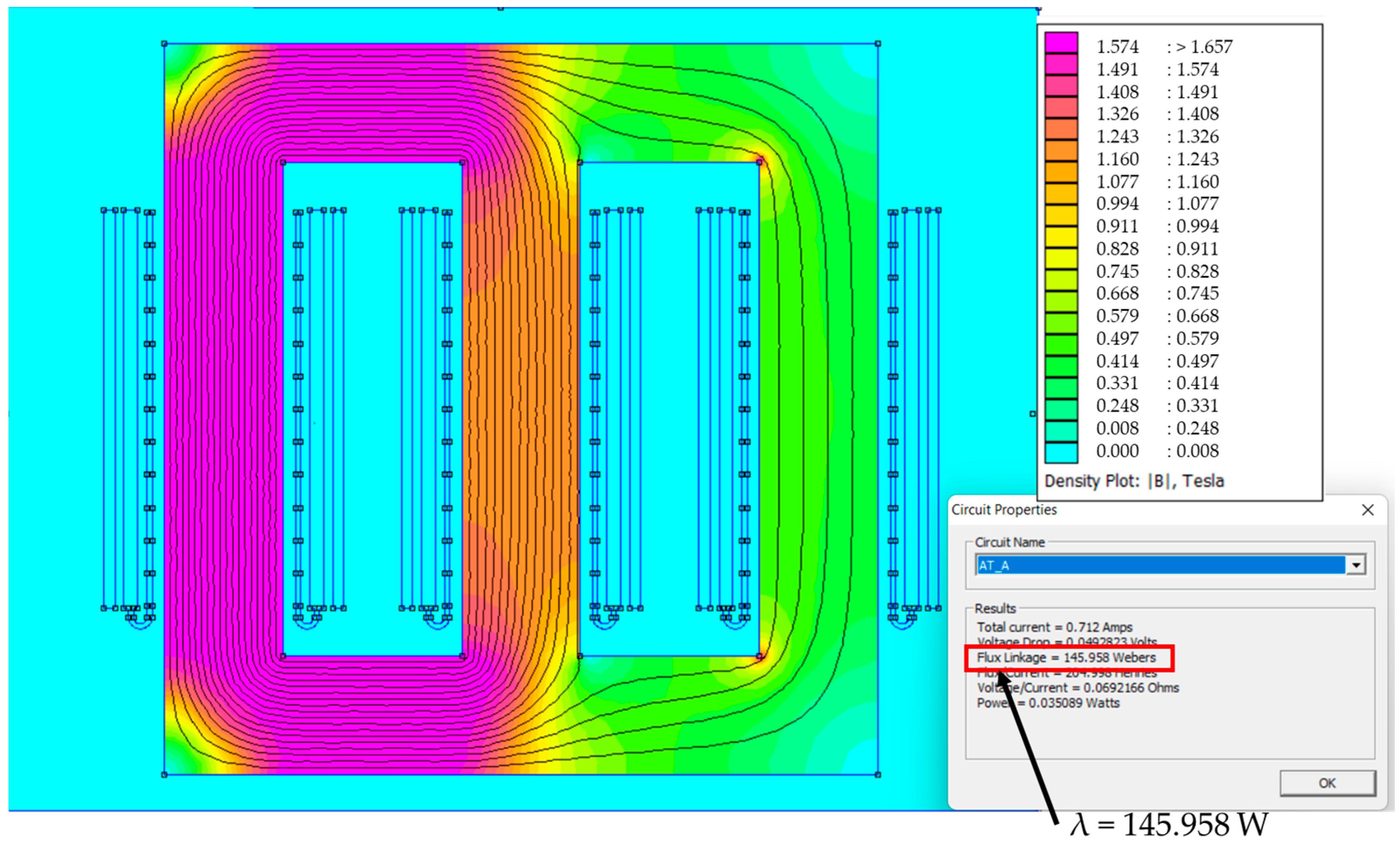
3.2.3. Magnetizing Inductance
3.2.4. Capacitance
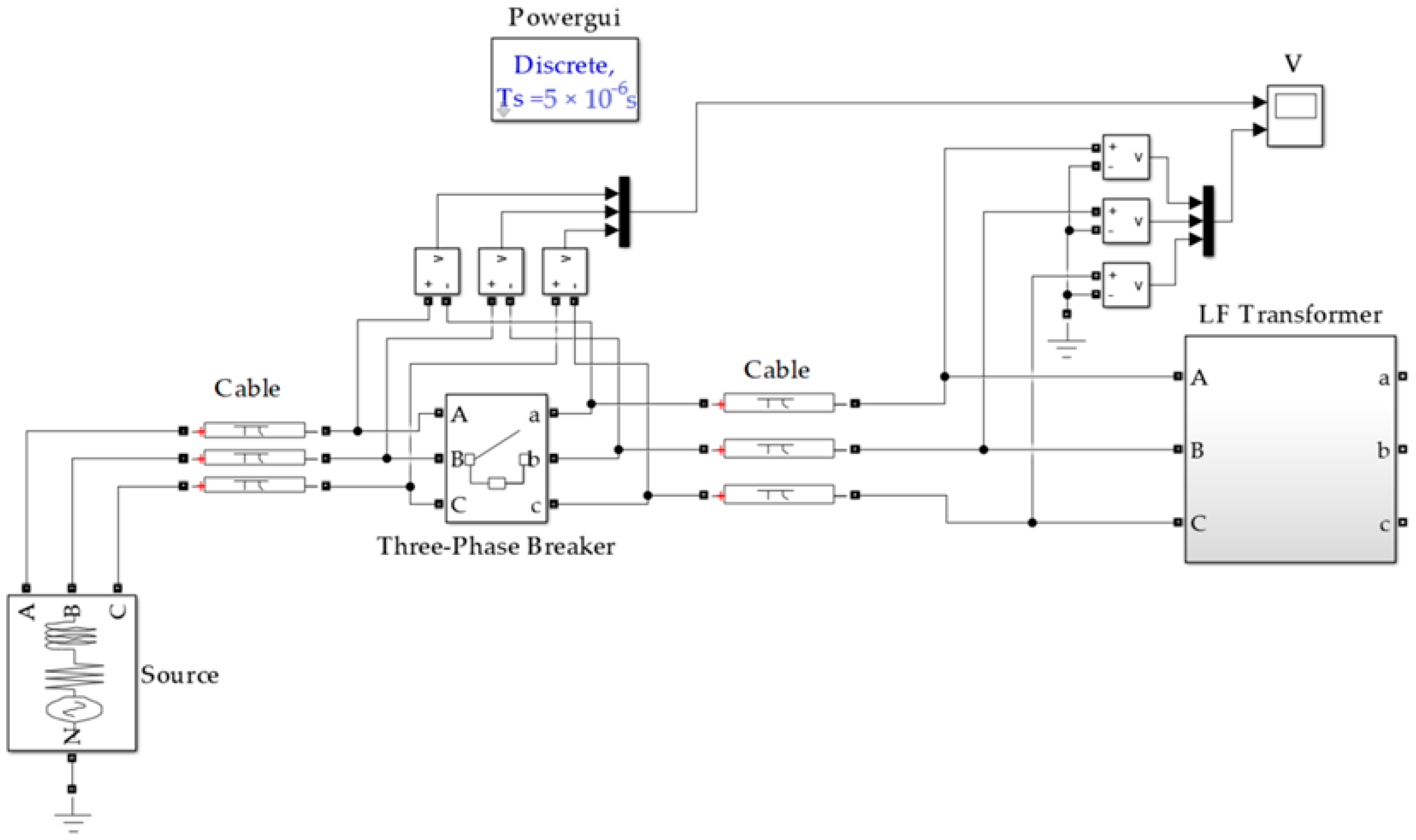
3.3. Tests Parameters Measurement
3.3.1. Load Loss Test
3.3.2. No Load Loss Test
3.3.3. Power Factor Test
4. Results and Discussion
5. Conclusions
Author Contributions
Funding
Data Availability Statement
Conflicts of Interest
References
- Christin, A.J.; Salam, M.A.; Rahman, Q.M.; Wen, F.; Ang, S.P.; Voon, W. Causes of transformer failures and diagnostic methods—A review. Renew. Sustain. Energy Rev. 2018, 82, 1442–1456. [Google Scholar] [CrossRef]
- Ramirez, J.M.V. Optimized Insulation Design of Power Transformer Windings Under Fast Voltage Pulses. Ph.D. Thesis, Western Michigan University, Kalamazoo, MI, USA, 2021. [Google Scholar]
- Tenbohlen, S.; Jagers, J.; Vahidi, F.; Cigre, W.G. A2.37—Standardized Survey of Transformer Reliability. In Proceedings of the 2017 International Symposium on Electrical Insulating Materials (ISEIM), Toyohashi, Japan, 11–15 September 2017. [Google Scholar]
- Singh, J.; Singh, S. Transformer Failure Analysis: Reasons and Methods. Int. J. Eng. Res. 2016, 4, 1–5. [Google Scholar]
- Harlow, J.H. (Ed.) Electric Power Transformer Engineering, 3rd ed.; CRC Press: Boca Raton, FL, USA, 2017. [Google Scholar]
- Marchi, B.; Zanoni, S.; Mazzoldi, L.; Reboldi, R. Energy Efficient EAF Transformer—A Holistic Life Cycle Cost Approach. Procedia CIRP 2016, 48, 319–324. [Google Scholar] [CrossRef]
- Marchi, B.; Zanoni, S.; Mazzoldi, L.; Reboldi, R. Product-service System for Sustainable EAF Transformers: Real Operation Conditions and Maintenance Impacts on the Life-cycle Cost. Procedia CIRP 2016, 47, 72–77. [Google Scholar] [CrossRef]
- Maia, T.A.C.; Onofri, V.C. Survey on the electric arc furnace and ladle furnace electric system. Ironmak. Steelmak. 2022, 49, 976–994. [Google Scholar] [CrossRef]
- Karandaeva, O.I.; Yakimov, I.A.; Filimonova, A.A.; Gartlib, E.A.; Yachikov, I.M. Stating Diagnosis of Current State of Electric Furnace Transformer on the Basis of Analysis of Partial Discharges. Machines 2019, 7, 77. [Google Scholar] [CrossRef]
- Radionov, A.A.; Liubimov, I.V.; Yachikov, I.M.; Abdulveleev, I.R.; Khramshina, E.A.; Karandaev, A.S. Method for Forecasting the Remaining Useful Life of a Furnace Transformer Based on Online Monitoring Data. Energies 2023, 16, 4630. [Google Scholar] [CrossRef]
- Sun, P.; Sima, W.; Jiang, X.; Zhang, D.; He, J.; Ye, L. Review of accumulative failure of winding insulation subjected to repetitive impulse voltages. High Volt. 2019, 4, 1. [Google Scholar] [CrossRef]
- Del Vecchio, R.M.; Poulin, B.; Feghali, P.T.; Shah, D.M.; Ahuja, R. Transformer Design Principles: With Applications to Core-Form Power Transformers, 3rd ed.; Taylor & Francis Group: Boca Raton, FL, USA; CRC Press: Boca Raton, FL, USA, 2017. [Google Scholar]
- Heathcote, M.J.; Franklin, D.P. The J & P Transformer Book: A Practical Technology of the Power Transformer, 12th ed.; Newnes: Oxford, UK; Boston, MA, USA, 1998. [Google Scholar]
- Mbetmi, G.-D.F.; Tchatchueng, F.T.; Andre, B.; Ngong, S.M.; Stephane, N.N. Mathematical models of power transformers winding faults diagnosis based on voltage-current characteristics. Int. J. Eng. Technol. 2024, 13, 156–166. [Google Scholar] [CrossRef]
- León-Martínez, V.; Peñalvo-López, E.; Andrada-Monrós, C.; Sáiz-Jiménez, J.Á. Load Losses and Short-Circuit Resistances of Distribution Transformers According to IEEE Standard C57.110′. Inventions 2023, 8, 154. [Google Scholar] [CrossRef]
- Katende, F.; Katende, J. Determination of Per-Phase Equivalent Circuit Parameters of Three-Phase Transformer Using MATLAB/Simulink. In Proceedings of the 2022 IST-Africa Conference (IST-Africa), Online, 16–20 May 2022; IEEE: New York, NY, USA, 2022; 8p. [Google Scholar] [CrossRef]
- Corrêa, H.P.; Vieira, F.H.T. An Approach to Steady-State Power Transformer Modeling Considering Direct Current Resistance Test Measurements. Sensors 2021, 21, 6284. [Google Scholar] [CrossRef] [PubMed]
- CIGRE WG 33.02. Guidelines for Representation of Network Elements When Calculating Transient; CIGRE: Paris, France, 1990. [Google Scholar]
- Martinez-Velasco, J. (Ed.) Transient Analysis of Power Systems: A Practical Approach; John Wiley & Sons: Hoboken, NJ, USA, 2020. [Google Scholar]
- Høidalen, H.K.; Rocha, A.C.O. Analysis of gray Box Modelling of Transformers. Electr. Power Syst. Res. 2021, 197, 107266. [Google Scholar] [CrossRef]
- Lazzari, E.F.; de Morais, A.P.; Ramos, M.; Ferraz, R.; Marchesan, T.; Bender, V.C.; Carraro, R.; Fontoura, H.; Correa, C.; Resener, M. A Comprehensive Review on Transient Recovery Voltage in Power Systems: Models, Standardizations and Analysis. Energies 2023, 16, 6348. [Google Scholar] [CrossRef]
- Matlab Documentation. 2024. Available online: https://www.mathworks.com/help/matlab/ (accessed on 15 April 2024).
- Aperam. Aços Elétricos de Grão Orientado Ficha; Técnica H110-27′; Aperam: Luxembourg, 2020. [Google Scholar]
- Meeker, D. Finite Element Method Magnetics—Version 4.2 Users Manual. 30 January 2018. Available online: https://www.femm.info/wiki/Documentation/ (accessed on 23 February 2020).
- ABNT NBR 5356. ABNT NBR 5356—Norma Brasileira de Transformadores de Potência; Normas: Sao Paulo, Brazil, 2007. [Google Scholar]
- IEEE Std C57.12.90; IEEE Standard Test Code for Liquid Immer. IEEE: New York, NY, USA, 2015.
- Flanagan, W. Transformer Design and Application Handbook, 2nd ed.; McGraw-Hill, Inc.: New York, NY, USA, 1993. [Google Scholar]
- Martignoni, A. Transformadores, 8th ed.; Editora Globo: Porto Alegre, Brazil, 2003. [Google Scholar]
- IEC 60317-0-2:2020; Specifications for Particular Types of Winding Wires—Part 0-2: General Requirements—Enamelled Rectangular Copper Wire. IEC: Geneva, Switzerland, 2020.
- Saraiva, E.; Chaves, M.L.R.; Camacho, J.R.; Caixeta, G. Adjustments for a Three-Phase Distribution Transformer Two-Dimensional Representation with Finite Element Method. In Proceedings of the 2nd International Symposium on Search Based Software Engineering (SSBSE 2010), Benevento, Italy, 7–9 September 2010. [Google Scholar]


| Origin | Frequency Ranges | Type of Transient |
|---|---|---|
| Ferroresonance | 0.1 Hz to 1 kHz | Low frequency |
| Load rejection | 0.1 Hz to 3 kHz | Low frequency |
| Fault clearing | 50 Hz to 3 kHz | Low frequency |
| Line Switching | 50 Hz to 20 kHz | Slow front |
| Lightning Overvoltage | 10 kHz to 3 MHz | Fast front |
| Switching in GIS | 100 kHz to 50 MHz | Very fast front |
| Variable | Value |
|---|---|
| Rated power | 33 MVA |
| Rated frequency | 60 Hz |
| Winding connection | Yd1 |
| Primary voltage | 69 kV |
| Secondary voltages | 437…329 V (13 TAPs) |
| No-load current at high voltage | 0.83 ARMS at 13° TAP |
| No-load losses | 33 kW at 13° TAP |
| Core specification | H110-27 oriented grain silicon steel (Aperam) [23] |
| Rated operating magnetic flux density | 1.67 T |
| Core cross-section area | 0.24522 m2 |
| Measured Values During Test | |
| VSC_1Ø (V) | 4327 |
| ISC (A) | 292.86 |
| Pr (W) | 151,051 |
| Pa (W) | 22,660 |
| Psc (W) | 173,711 |
| Calculated Values | |
| NHV/NLV | 91 |
| RHV (Ω) | 0.197 |
| RLV (Ω) | 0.00004 |
| LHV (H) | 0.01131 |
| LLV (H) | 1.3661 × 10⁻⁶ |
| Measured Values During Test | |
| V0_1Ø (V) | 438 |
| I0 (A) | 50.87 |
| P0 (W) | 28,942 |
| Calculated Values | |
| NHV/ NLV | 91 |
| Rm_HV (Ω) | 164,673.5 |
| Lm_HV (H) | 209.8 |
| Tests Measurement | Analytical Calculation | Finite Element Analysis (FEA) | |
|---|---|---|---|
| RHV (Ω) | 0.197 | 0.1927 | 0.1928 |
| RLV (Ω) | 0.00004 | 3.929 × 10⁻⁵ | 3.93 × 10⁻⁵ |
| LHV (H) | 0.0113 | 0.0104 | 0.0103 |
| LLV (H) | 1.36 × 10⁻⁶ | 1.26 × 10⁻⁶ | 1.25 × 10⁻⁶ |
| Rm_HV (Ω) | 164,673.5 | 175,670 | − |
| CHV_LV (F) | 2.75 × 10⁻⁹ | 2.61× 10⁻⁹ | 2.625 × 10⁻⁹ |
| CHV_G (F) | 2.18 × 10⁻⁹ | 2.30 × 10⁻⁹ | 2.29 × 10⁻⁹ |
| CLV_G (F) | 2.8 × 10⁻⁹ | 3.03 × 10⁻⁹ | 3.04 × 10⁻⁹ |
| FEA vs. Tests Measurement | FEA vs. Analytical Calculation | |
|---|---|---|
| RHV (Ω) | 2.13% | −0.05% |
| RLV (Ω) | 1.75% | −0.03% |
| LHV (H) | 8.25% | 0.96% |
| LLV (H) | 8.1% | 0.8% |
| Rm_HV (Ω) | - | - |
| CHV_LV (F) | −4.5% | −0.57% |
| CHV_G (F) | −5.05% | 0.43% |
| CLV_G (F) | −8.57% | −0.33% |
Disclaimer/Publisher’s Note: The statements, opinions and data contained in all publications are solely those of the individual author(s) and contributor(s) and not of MDPI and/or the editor(s). MDPI and/or the editor(s) disclaim responsibility for any injury to people or property resulting from any ideas, methods, instructions or products referred to in the content. |
© 2024 by the authors. Licensee MDPI, Basel, Switzerland. This article is an open access article distributed under the terms and conditions of the Creative Commons Attribution (CC BY) license (https://creativecommons.org/licenses/by/4.0/).
Share and Cite
Onofri, V.C.; Maia, T.A.C.; Filho, B.J.C. Assessment of Non-Linear Modeling of Ladle Furnace Transformer Using Finite Element Analysis. Machines 2024, 12, 900. https://doi.org/10.3390/machines12120900
Onofri VC, Maia TAC, Filho BJC. Assessment of Non-Linear Modeling of Ladle Furnace Transformer Using Finite Element Analysis. Machines. 2024; 12(12):900. https://doi.org/10.3390/machines12120900
Chicago/Turabian StyleOnofri, Virna Costa, Thales Alexandre Carvalho Maia, and Braz J. Cardoso Filho. 2024. "Assessment of Non-Linear Modeling of Ladle Furnace Transformer Using Finite Element Analysis" Machines 12, no. 12: 900. https://doi.org/10.3390/machines12120900
APA StyleOnofri, V. C., Maia, T. A. C., & Filho, B. J. C. (2024). Assessment of Non-Linear Modeling of Ladle Furnace Transformer Using Finite Element Analysis. Machines, 12(12), 900. https://doi.org/10.3390/machines12120900