Concurrent AI Tuning of a Double-Loop Controller for Multi-Phase Drives

Abstract

The control of electric drives is an important topic due to the wide-spread use of such devices. Among these, multi-phase induction machines are gaining momentum in variable-speed applications. The usual control practice is the use of a speed Proportional–Integral loop that sets the current reference for an inner controller. This inner controller decides the voltage to be applied, which is realized by an electronic power converter. This paper presents an Artificial Intelligence (AI) scheme for tuning. It aims to optimize the usual figures of merit for drives. Moreover, tuning for both loops is tackled concurrently. The adjustment is performed relying on the operating region to address non-linear behavior. The results obtained using a five-phase induction motor illustrate that the proposed method can work in the entire operating range of the drive with improved results.

1. Introduction

Advanced control methods for induction machines (IMs) employ a two-loop configuration scheme, including a loop responsible for generating electro-magnetic torque and an outer loop that incorporates a speed feedback mechanism [1]. In this outer loop, a PI (proportional action plus integral action) is frequently found, whose output represents the torque and flux references for the inner control loop that are decomposed into orthogonal stator current components. These stator setpoints are then used by the inner controller to switch on a Voltage Source Inverter (VSI) and achieve a defined control goal. The switching power converter that represents the VSI takes the incoming DC voltage to generate AC voltage using discrete switching methods such as space vector or pulse width modulation techniques. Current control can be also performed through the predictive control of VSI states [2]. The predictive method constitutes so called Finite-State Model Predictive Control (FSMPC). This method has been utilized for various systems. The case of multi-phase drives is interesting [1]. In multi-phase drives, FSMPC deals with a larger phase number [3]. Another positive trait is their ability to cope with different electrical objectives, such as the minimization of the current ripple, the commutation losses or the harmonic content [4]. This is achieved through cost function (CF) design, which involves the subsequent tuning of weighting factors (WFs) that appear in the CF [5].

Different factors appear in multi-phase control performance [6]. Previous works have recognized the problem of CF tuning [7], where a specific compromise solution should be identified to avoid the conflicting nature of the objectives [8]. For example, the understanding that it is not possible to simultaneously enhance all performance metrics is illustrated for a six-phase machine in [9] using a Pareto diagram. This result led researchers to create techniques to adjust the cost function of FSMPC within the inner loop (see [10]). Therefore, soft constraints are applied in [11] for a multiphase IM with nine phases. However, this method does not address the matter of dependence on the operating points. Although the proposal of [9] uses fixed WFs, different performance metrics, operating conditions and figures of merit are taken into account. In [12], a Lyapunov method is used for a multilevel rectifier; it is unclear how to adapt it to AC drives. Finally, in [13], WF tuning is performed for a six-phase system using the model reference approach. However, a speed loop is not incorporated.

Artificial Intelligence (AI) methods have been proposed for drives, mainly considering just the mechanical side; thus, the elements in the inner loop (power converter, modulation methods, etc.) are considered ideal. Early works deal with replacing the speed control PI with a non-linear block such as a fuzzy or neural network (NN) system [14]. Reinforcement learning (RL) has also found an application in the speed tracking of brushless electrical machines, where PID tuning is updated according to a deterministic policy gradient algorithm [15]. A similar objective is pursued in [16], where a wavelet-based fuzzy adaptive algorithm is used to set the PID parameters of a brushless DC motor. In [17], an echo state network and the swarm method are utilized to model the dynamics of a permanent magnet motor. Similarly, in [18], a data-driven approach based on a long–short-term memory NN is employed. An off-line phase is used to obtain a control map that is later realized with another neural network. Changes in system dynamics due to changes in the operating point are mostly not considered [19,20].

Continuing with electro-magnetic variables, but in the realm of drives, AI techniques have been reported for various tasks. For example, and with respect to modeling, in [21], neural models are compared with the first principles for their use in the FSMPC of a three-phase permanent magnet drive. Delays and other nonidealities are considered in [22]. The work of [23] uses a first-order Taylor expansion of a maximum-torque-per-ampere policy of a permanent magnet motor in a simulation. Regarding the controllers themselves, in [24], a neural controller is trained to mimic a predictive speed controller. Similarly, [25] presents a predictive scheme for the inner loop but relies on modulation instead of FSMPC. The speed loop overshoot is mitigated in [26] by implementing a kernel controller. Furthermore, the research conducted in [27] introduces an observer for disturbances in sliding control. The current reference is sent to FSMPC and adaptive tuning is used for the WF.

In the more focused realm of AI approaches for IM control, some works such as [28] deal with the elimination of weighting factors. The authors of the current study have argued against this, since the WF provides flexibility to pursue different objectives to various degrees. This idea is shared by other researchers who have proposed methods for WF tuning, such as [29]. In this vein, ref. [30] proposes fuzzy control and WFs to mitigate speed/torque fluctuations. While speed is taken into account, load is not addressed. Nonetheless, the contribution is noteworthy, as it incorporates various performance metrics that were not considered in earlier studies.

Novelty and Contributions

As follows from the state of the art, the problem of the concurrent tuning of both loops for multi-phase induction machines remains unsolved. The originality of the proposed method lies in solving concurrent tuning by means of an AI approach. This is the principal objective of this work. The contributions of this work are briefly explained below.

• An automatic and on-line method for the adjustment of all controller parameters is proposed.
• All parts of the drive (electro-magnetic and mechanical) are considered in a holistic way.
• The weighting factors of FSMPC are retained as degrees of freedom for the consideration of different objectives (figures of merit).
• The whole sinusoidal steady-state operation space of the drive is considered to include combinations of speed and load.
• Flexibility to adapt to different applications is achieved through the use of a customizable optimization problem.
• An assessment in a real five-phase IM is presented considering computational and experimental issues.

The next section presents the formulation of the problem along with the essential theoretical framework. The proposed method is introduced in Section 3 and later put to the test using a laboratory setup in Section 4.

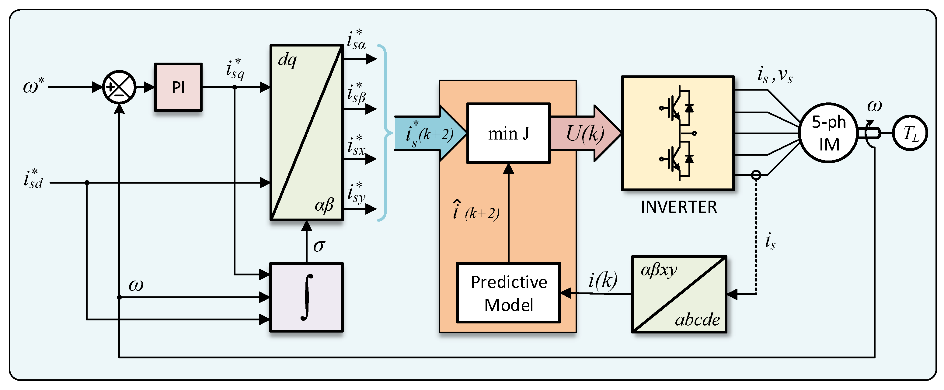
2. FSMPC Control of IM

Some background material is now presented to describe the context of the proposed method. Please note that, the proposed method is applicable to any multi-phase IM; however, this section specifically focuses on a five-phase IM for concretion. The diagram in Figure 1 shows the main elements of FSMPC: the speed and stator current controllers, the VSI and the multi-phase IM.

The VSI can generate 32 different voltages. These are produced by the distinct states of the switches. The ON or OFF state of the top switch of leg i is designed as $u_i$; then, the stator voltage of the phases is $V_{ph}=TU$, where $V_{ph}=(v_1,...,v_5)$, $U=(u_1,...,u_5)$, and T is defined as follows.

$$T={\displaystyle \frac{V_{DC}}{5}}\left(\begin{array}{ccccc}\hfill 4& -1& -1\hfill & -1& -1\\ \hfill -1& 4& -1\hfill & -1& -1\\ \hfill -1& -1& 4\hfill & -1& -1\\ \hfill -1& -1& -1\hfill & 4& -1\\ \hfill -1& -1& -1\hfill & -1& 4\end{array}\right),$$

(1)

where $V_{DC}$ is the voltage of the DC link. It is interesting to mention that a five-phase IM is generally represented, for clarity and simplicity, using two orthogonal planes, $\alpha -\beta$ and $x-y$. Note that while the $\alpha -\beta$ components are related to the production of flux/torque in the machine, the components $x-y$ are related to losses. The Clarke transformation is used to obtain the $\alpha$, $\beta$x and y components. The transformation is provided by:

$$M={\displaystyle \frac{2}{5}}\left(\begin{array}{rrrrr}\hfill 1& cos\vartheta & cos2\vartheta \hfill & cos3\vartheta & cos4\vartheta \\ \hfill 0& sin\vartheta & sin2\vartheta & sin3\vartheta & sin4\vartheta \\ \hfill 1& cos2\vartheta & cos4\vartheta & cos\vartheta & cos3\vartheta \\ \hfill 0& sin2\vartheta & sin4\vartheta & sin\vartheta & sin3\vartheta \\ \hfill 1/2& 1/2& 1/2& 1/2& 1/2\end{array}\right),$$

(2)

where $\vartheta =\pi /5$.

The indirect field-oriented control (IFOC) scheme uses quantities in the rotating $d-q$ reference frame. The d component deals with the generation of rotor flux. The q axis is related to electrical torque. The Park matrix is utilized to transform $\alpha -\beta$ axes into $d-q$ with the equation $V_{d-q}=D{V}_{\alpha \beta xy}$, with

$$D=\left(\begin{array}{cc}\hfill cos\sigma & sin\sigma \\ \hfill -sin\sigma & cos\sigma \end{array}\right).$$

(3)

In matrix D, angle $\sigma$ is the flux position, computed as $\sigma =\int {\omega }_{r}dt$, where ${\omega }_r$ is the rotor electrical speed, computed as ${\omega }_r={\omega }_{sl}+P{\omega }^e$, and P is the pole-pair number. The quantity ${\omega }^e$ is the estimation of mechanical speed obtained from the encoders, whereas ${\omega }_{sl}$ represents the slip speed. A setpoint for $d-q$ intensities is provided by a PI with proportional gain $k_p$, and integral gain $k_i$ is used for this purpose. This PI controller produces

$$\begin{array}{c}\hfill i_q^{*}\left(t\right)=k_p·e_{\omega }\left(t\right)+k_i{\int }_0^t{e}_{\omega }\left(\tau \right)d\tau \end{array}$$

(4)

where $e_{\omega }$ is the control error in mechanical speed, computed as $e_{\omega }\left(t\right)={\omega }^{*}\left(t\right)-{\omega }^e\left(t\right)$, where ${\omega }^{*}$ is the commanded or reference speed.

The control of the stator currents is done in the $\alpha -\beta -x-y$ planes. To do so, the reference $i_{dq}^{*}$ obtained from (4) is transformed to the $\alpha \beta xy$ axes by means of

$$\begin{array}{c}\hfill i_{\alpha }^{*}\left(t\right)=I^{*}sin{\omega }_{e}t,i_{\beta }^{*}\left(t\right)=I^{*}cos{\omega }_{e}t,i_x^{*}\left(t\right)=0,i_y^{*}\left(t\right)=0,I^{*}=\parallel i_{dq}^{*}\parallel .\end{array}$$

(5)

This results in the usual sinusoidal reference for $\alpha \beta$ and zero reference for $xy$ [10]. FSMPC aims at tracking the reference $i_{\alpha \beta xy}^{*}$. This is achieved using the usual MPC method, minimizing the cost function. The model provides predictions as follows:

$${\widehat{i}}_{\alpha \beta xy}(k+1)=\mathsf{\Phi }\left(\omega \right)i_{\alpha \beta xy}\left(k\right)+\mathsf{\Psi }U\left(k\right),$$

(6)

where $\mathsf{\Phi }$ and $\mathsf{\Psi }$ are matrices obtained from IM modeling and discretization [1], and U is the control action already defined in terms of the state of switches in the VSI. Please note that temperature changes and other effects may produce changes in the model. Identification and adaptation methods can be used to track such changes [31]. The computations introduce a delay, prompting the use of a second prediction computed as ${\widehat{i}}_{\alpha \beta xy}(k+2)=\mathsf{\Phi }\left(\omega \right){\widehat{i}}_{\alpha \beta xy}(k+1)+\mathsf{\Psi }U(k+1)$. In this way, the control action $U(k+1)$ is obtained at time k, minimizing J. This CF consists of several terms. Penalties are placed for predicted errors in $\alpha -\beta$, $x-y$ and VSI switching. This is mathematically expressed as

$$J=\parallel {\widehat{E}}_{\alpha \beta }{(k+2)\parallel }^2+{\lambda }_{xy}{\parallel {\widehat{E}}_{xy}(k+2)\parallel }^2+{\lambda }_{sc}SC(k+1)$$

(7)

where $\parallel {\widehat{E}}_{\alpha \beta }{\parallel }^2$ is the root-mean-squared control error in the $\alpha -\beta$ subspace, $\parallel {\widehat{E}}_{xy}{\parallel }^2$ is the root-mean-squared control error in the $x-y$ subspace and $SC$ is the sum of all changes in the power switches of the VSI:

$$SC(k+1)=\sum _{h=1}^5|u_h(k+1)-u_h\left(k\right)|$$

(8)

where the absolute value of $u_h(k+1)-u_h\left(k\right)$ represents the changes in power switches at the VSI due to the application of the candidate control action $u(k+1)$ made at k.

The WFs of the CF are the parameters ${\lambda }_{xy}$ and ${\lambda }_{sc}$ and have to be tuned considering performance indicators, as presented in Section 2.1.

2.1. Figures of Merit

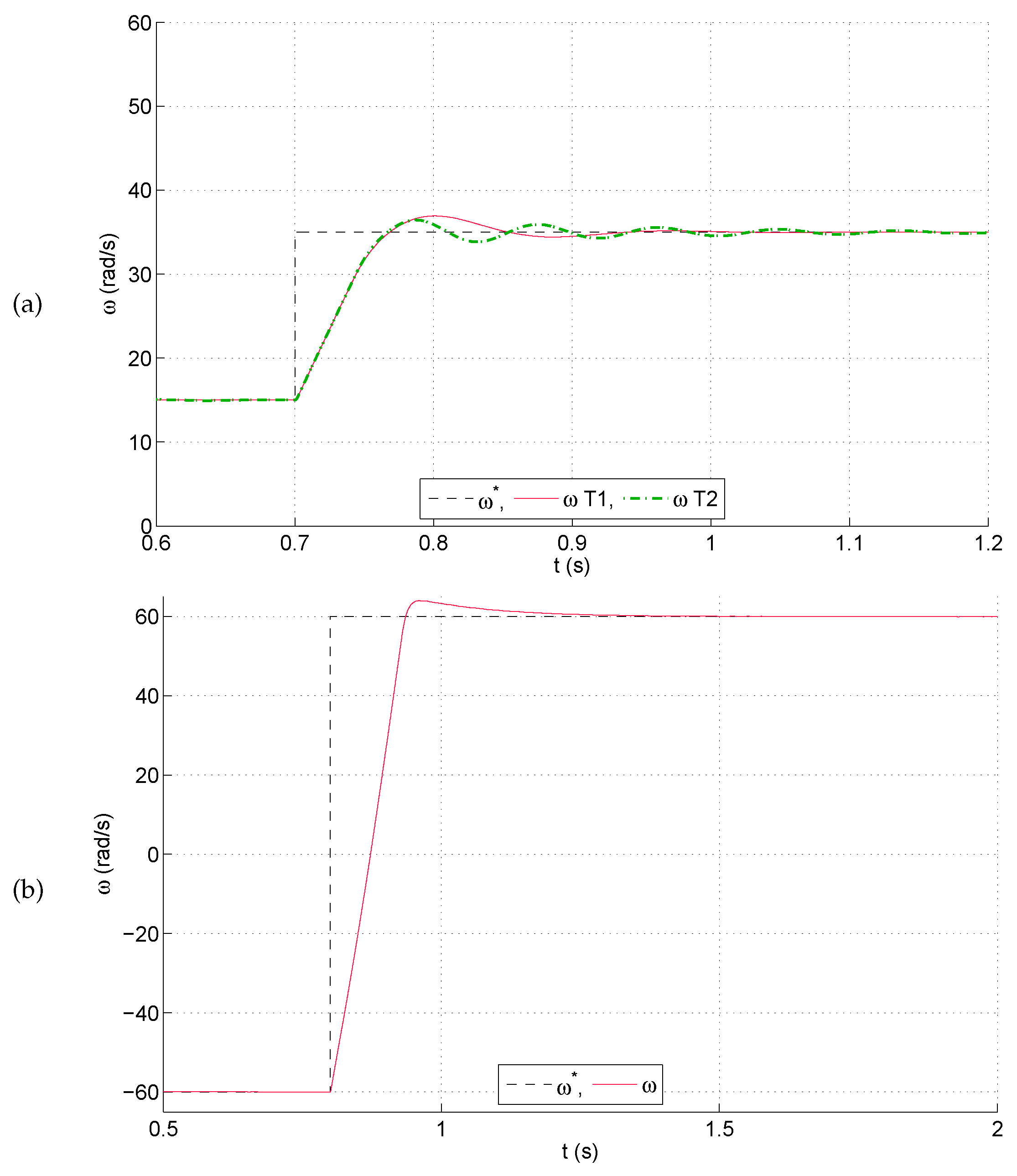
The control objectives depend upon the actual application for the drive. For instance, traction applications may require different values for overshoot than a pump. In the experimental section, a certain prioritization of control objectives is used just to showcase the capabilities of the proposed method. Also, a handful of the most commonly found objectives $\pi$ are presented below.

• Overshoot in mechanical speed (${\pi }_1=PO$). This is defined as per (9), and is something to avoid.
• Mechanical speed rise time (${\pi }_2=T_r$). This is defined as per (10), and should be low enough to provide a fast dynamic response of the drive. It is usually in conflict with $PO$, so in most cases, a compromise solution must be found.
• The absolute error of the integral time (${\pi }_3=ITAE$) penalizes the duration of the tracking error. This is defined as per (11) and is applied to the mechanical speed.
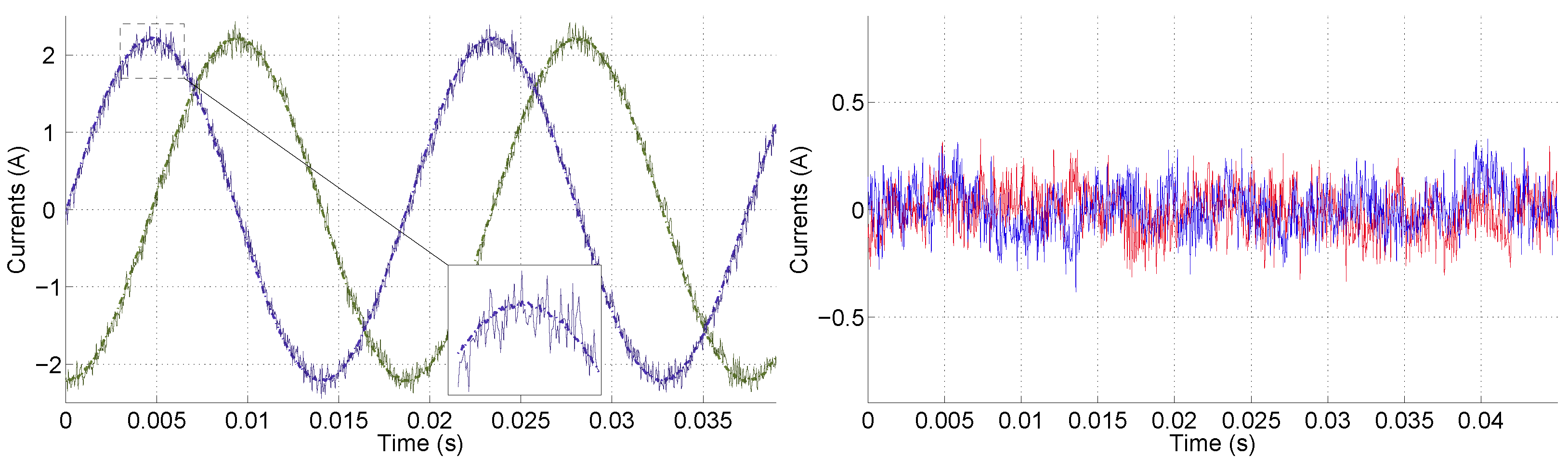
• Torque ripple (${\pi }_4=R_t$). This is defined as per (12) and is actually an electro-magnetic quantity directly generated by stator currents. It is a cause for mechanical stress, so it has to be avoided.
• Harmonic content (${\pi }_5=E_{xy}$). This is defined as per (13) and must be kept as low as possible as it contributes to losses.
• Average value for the switching frequency (${\pi }_6=ASF$). This is defined as per (14) and must be maintained within suitable limits to avoid losses and damages to the VSI.

The performance indices are defined in mathematical terms as follows.

$$\begin{array}{ccc}\hfill PO& =& 100·{\displaystyle \frac{max\omega -{\omega }^{*}}{{\omega }^{*}}}\hfill \end{array}$$

(9)

$$\begin{array}{ccc}\hfill T_r& =& \underset{t\ge 0}{argmin}{\omega }^{*}\left(t\right)-\omega \left(t\right)\hfill \end{array}$$

(10)

$$\begin{array}{ccc}\hfill ITAE& =& {\displaystyle \frac{1}{N}}\sum _{k=1}^N{\displaystyle \frac{\parallel {\omega }^{*}\left(k\right)-\omega \left(k\right)\parallel }{{\omega }^{*}\left(k\right)}}k\hfill \end{array}$$

(11)

$$\begin{array}{ccc}\hfill R_t& =& \sqrt{{\displaystyle \frac{1}{N}}\sum _{k=1}^N{\left(T^{*}\left(k\right)-T\left(k\right)\right)}^2}\hfill \end{array}$$

(12)

$$\begin{array}{ccc}\hfill E_{xy}& =& \sqrt{{\displaystyle \frac{1}{N}}\sum _{k=1}^N{e}_{xy}^2\left(k\right)}\hfill \end{array}$$

(13)

$$\begin{array}{ccc}\hfill ASF& =& {\displaystyle \frac{1}{5N{T}_s}}\sum _{k=1}^{N}SC\left(k\right)\hfill \end{array}$$

(14)

These expressions are commonplace in papers dealing with drives.

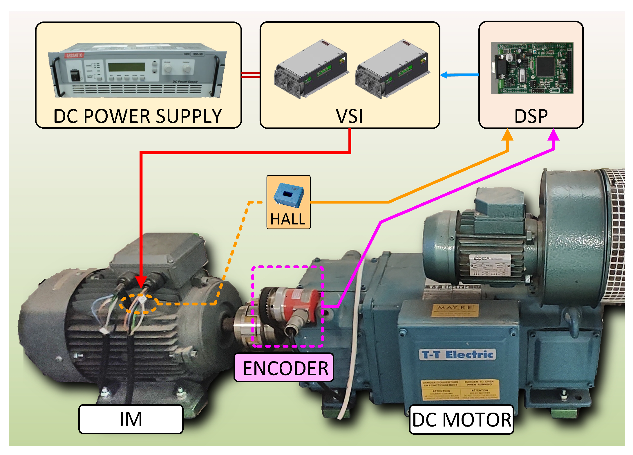
2.2. Experimental Setup

A testing work bench was used to obtain training data for the AI-based tuner and also to evaluate the tuned system, with tests carried on a five-phase IM.

The experimental setup included a five-phase IM and sensing and control elements, as presented in Figure 2. The main parameters are provided in

Table 1. Parameters of experimental 5-phase IM.

Parameter	Value	Unit
Stator resistance, $R_s$	12.85	$\mathsf{\Omega }$
Rotor resistance, $R_r$	4.80	$\mathsf{\Omega }$
Stator leakage inductance, $L_{ls}$	79.93	mH
Rotor leakage inductance, $L_{lr}$	79.93	mH
Mutual inductance, $L_M$	681.7	mH
Rotational inertia, $J_m$	0.02	kg m2
Number of pairs of poles, P	3	-

. These parameters were obtained through identification, as described in [32].

The five-phase VSI is constructed from SKS 22F modules, and a DC link implemented with a KDC 300-50 power supply (Keysight, Colorado Springs, CO, USA). The core of the control unit is a TMS320F28335 digital signal processor (Texas Instruments, Dallas, TX, USA) on an MSK28335 board (Technosoft, Blue Ash, OH, USA), where the control program runs in real time. A GHM510296R/2500 encoder (Sensata Technologies, Attleboro, MA, USA) provides the feedback of the mechanical speed signal. The load can be provided by a co-axial direct-current motor.

3. Proposed ANN Tuning Method

The proposed method is illustrated in the diagram in Figure 3. It consists of an artificial neural network (ANN) that provides the optimal PI controller parameters and optimal FSMPC weighting factors according to the actual speed $\omega$ and its reference ${\omega }^{*}$. Denoting the set of parameter as $\theta$

$$\theta =\left(k_p,k_i,{\lambda }_{xy},{\lambda }_{sc}\right),$$

(15)

the ANN’s task is to compute ${\theta }^{*}=\mathrm{f}(\omega ,{\omega }^{*})$. The ANN was chosen because of its universal approximation property. Other approximators could be used as well. The simplicity of the perceptron facilitates its implementation in many control hardware platforms such as Field-Programmable Gate Arrays. The network architecture is a multilayer perceptron with sigmoidal activation in the hidden units, linear activation in the output units and bias connections to all units. The scheme for this type of ANN is well known, and the interested reader can consult [33] for further details.

The network size is determined by cross-validation [33]. The best results are found for a medium-size ANN of two hidden layers with 20 and 10 units.

Network training uses early stopping and a final phase of validation [33]. The division of training data into sets for training, testing and validation is performed using simple random sampling. The percentage of data use for each set is the same since there is no shortage of data in this particular case.

The scheme in Figure 3 can be used for different applications. For each case, the objectives and restrictions have to be dealt with.

3.1. Objectives and Restrictions

Different applications of the drive might require different values for the performance indices. For concretion, a particular case is used here where overshoot and VSI switching frequency are given priority. This case can be tackled with the help of the following optimization problem:

$$\begin{array}{cccc}\hfill & \underset{\theta }{min}\hfill & \hfill & c_2{\pi }_2+c_3{\pi }_3+c_4{\pi }_4+c_5{\pi }_5\hfill \\ \hfill & \mathrm{s}.\mathrm{t}.\hfill & \hfill & {\pi }_1\le U_{PO}\hfill \\ \hfill & \hfill & & {\pi }_6\le U_{ASF}.\hfill \end{array}$$

(16)

The function being optimized $\mathsf{\Xi }=c_2{\pi }_2+c_3{\pi }_3+c_4{\pi }_4+c_5{\pi }_5$ is a combination of objectives. Coefficients $c_i$ must be designed according to the relative importance of each performance index. Also, those performance indices considered most important are treated as constraints. This is the case in (16) for $PO<U_{PO}$ and $ASF<U_{ASF}$. The first constraint ensures that the overshoot will be below the limit. The second constraint ensures that the VSI will not overheat and become damaged due to fast commutations. Please note that other optimization problems include possible interchanging constraints and terms in $\mathsf{\Xi }$. In this manner, it is possible to ensure some operational values (constraints) while minimizing the rest of the performance indicators (index $\mathsf{\Xi }$).

With these considerations, the training data generation is explained in the next part.

3.2. Data Gathering and Training

Supervised learning is used to obtain an ANN model that provides $\theta$ as a function of $x=(\omega ,{\omega }^{*})$. Training is achieved by selecting the most appropriate set of parameters for both loops. The needed data-set of input/output values is obtained by minimizing $\mathsf{\Xi }$ for a collection of operating points. The minimization is performed considering experimental data where pairs of $\mathsf{\Pi }$ values are gathered for each tentative $\theta$ and operating point.

The experimental $\mathsf{\Pi }$ values are gathered by performing step tests on the experimental setup. This task should consider the fact that a large number of $\theta$ combinations is possible. For instance, in a grid where each ${\theta }_i$ is divided into ten parts, ${10}^4$ combinations are possible for vector $\theta$. This number is affordable for a simulation but it is prohibitive for an experimental platform. Some techniques have been devised to reduce the number of experimental trials to obtain the training data.

• The outer PI loop can be roughly tuned using a simplified dynamical model corresponding to a second-order transfer function. This provides a set of initial guesses for ${\theta }_1$ and ${\theta }_2$ that are later refined.
• Similarly, an initial guess for the WF parameters of the CF can be obtained from previous works on IMs, as shown in [13]. This provides a set of initial guesses for ${\theta }_3$ and ${\theta }_4$.
• Finally, instead of the extensive exploration of $\theta$ space featured in previous works, gradient descent is used to produce new combinations from existing ones. In this way, the experimental setup can drive itself in the data-gathering task. This is similar to the strategy for real-time WF selection proposed in [13] for a six-phase IM.

This strategy is illustrated in the diagram in Figure 4, where $\mathsf{\Sigma }$ represents the whole drive under closed-loop control, using parameters dictated by $\theta$. The step tests have the form depicted in Figure 5, where a set of step changes are introduced in ${\omega }^{*}$ for every operating situation. In this way, different operating regimes are considered.

The controller tuning is initially set to ${\theta }^0$ and later changed after each step. This leads to convergence of the performance indicators towards appropriate values. The procedure is carried out for all operating regimes in the IM’s range. Each test requires less than a minute to complete, so in a few minutes, the whole operational range is covered.

With this strategy a set of input/output pairs is gathered for ANN training. A similar approach is used to derive another data-set for final testing using different values for ${\omega }^{*}$. Figure 6 shows a partial view of the data-set.

The network size is selected using the usual validation set and early stopping. The actual training is carried out using the Matlab Toolbox for shallow networks.

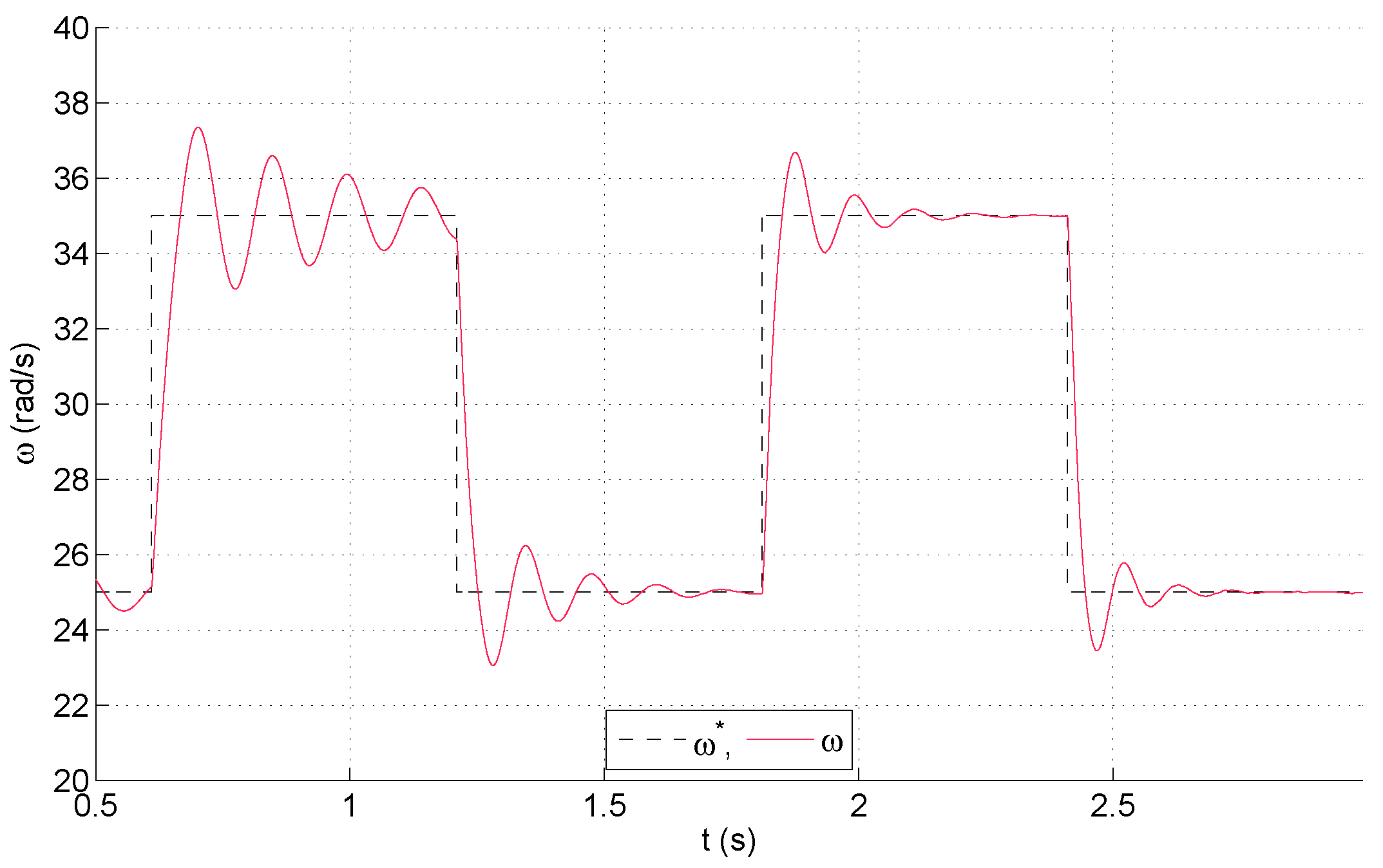
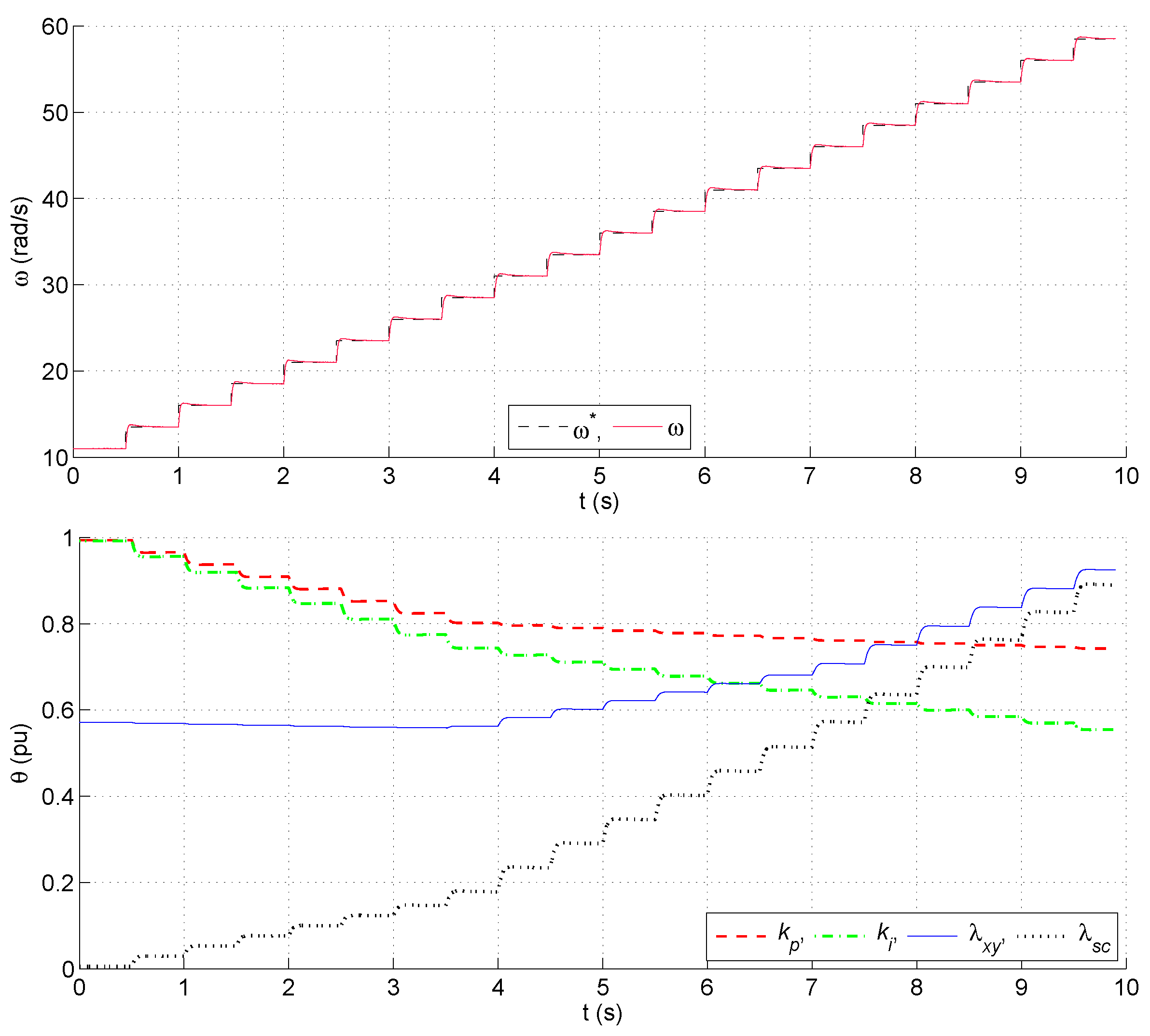
4. Experimental Results

Several tests are carried out in the benchmark for assessment. First, transient operation is considered, where a step is introduced in ${\omega }^{*}$. The performance indicators are gathered for two tunings: (A) and (B). The parameters for each tuning are provided in

Table 2. The tunings $\theta$ used for the comparison.

Speed	Ctrl	${\mathit{k}}_{\mathit{p}}·{10}^3$	${\mathit{k}}_{\mathit{i}}·{10}^5$	${\mathit{\lambda }}_{\mathbf{xy}}$	${\mathit{\lambda }}_{\mathbf{sc}}·{10}^4$
Low	A	295	8.3	0.15	1.60
Med	A	295	8.3	0.15	1.60
High	A	295	8.3	0.15	1.60
Low	B	387	12.3	0.12	0.00
Med	B	295	7.8	0.15	1.58
High	B	285	6.5	0.21	2.85

. The rationale for the tunings is explained below.

• Tuning (A) is a commonly found tuning in which the non-linearities produced by changes in the operating point are not realized. In particular ${\lambda }_{xy}$ and ${\lambda }_{sc}$ are set to low enough values to obtain acceptable values of $E_{xy}$ and $ASF$ on average. A fast response is sought with this tuning, achieving low values of $T_r$. This type of tuning is found in many published works.
• Tuning (B) corresponds to the proposed method, where $\theta =\mathrm{f}(\omega ,{\omega }^{*})$ is provided by an ANN. The constraints of (16) are set to $U_{PO}=9.6$ (%) and $U_{ASF}=10$ (kHz). Function $\mathsf{\Xi }$ uses the parameters $c_2=0.5/{\pi }_2^{max}$, $c_3=0.1/{\pi }_3^{max}$, $c_4=0.1/{\pi }_4^{max}$ and $c_5=0.3/{\pi }_5^{max}$. This tuning aims at ensuring proper working of the VSI, leading to a reduction in overshoot and maintaining a certain trade-off between performance indicators.

The results shown in

Table 3. The results obtained for standard tuning (A) and the proposed method (B).

		$\mathit{PO}$	${\mathit{T}}_{\mathit{r}}$	${\mathit{R}}_{\mathit{t}}$	$\mathit{ITAE}$	${\mathit{E}}_{\mathit{xy}}$	$\mathit{ASF}$	$\mathbf{\Xi }$
Speed	Ctrl	(%)	(ms)	(mNm)	-	(mA)	kHz	-
Low	A	9.4	834	23.3	24.2	23.9	3.85	0.99
Med	A	9.7	834	19.9	7.0	24.9	9.95	0.92
High	A	9.9	839	18.6	5.1	25.7	11.2	0.92
Low	B	9.5	823	24.2	15.0	24.2	6.71	0.95
Med	B	9.1	835	20.1	6.9	24.9	10.0	0.92
High	B	8.1	838	19.1	6.0	24.7	10.0	0.91

indicate the superiority of the concurrent tuning (case B) vs. the standard tuning (case A). To begin with, the constraints are satisfied with the proposed method. In case A, however, $PO$ is over the limit for low speeds and $ASF$ surpasses the 10 (KHz) mark for high speeds. On average, however, these violations do not occur. Also, with the proposed method, the performance indicators are balanced to produce the minimum possible values of $\mathsf{\Xi }$ for each speed. Again, the values for the standard tuning are higher. To further illustrate the performance of the proposed method, Figure 6 presents the mechanical speed for a series of step tests conforming to a stair-case. In this way, the step response is obtained for different operating regimes. It can be seen that the dynamic performance is maintained across all speeds. In Figure 6, the controller parameters are shown, clearly demonstrating the adaptation achieved by the ANN.

Notice that each ${\theta }_i$ is divided by ${\theta }_i^{max}$ to attain a per-unit representation. The max values are ${\theta }_1^{max}=0.387$, ${\theta }_2^{max}=1.23$ × ${10}^{-4}$, ${\theta }_3^{max}=0.21$ and ${\theta }_4^{max}=2.85$ × ${10}^{-4}$.

A second set of results is provided to illustrate the non-linear behavior and trade-offs existing in the drive. This is important, as different tunings ($\theta$) provide different performance indicators that are in conflict with each other. This is shown in Figure 7 by means of performance maps. These maps use $k_p$ and $k_i$ as axes. In this way, many different tunings can be assessed at once. From the maps, it can be seen that $PO$ and $R_t$ require almost opposite values for $k_p$ and $k_i$. This is easily discernible, as high values of $PO$ correspond to zones where $R_t$ is low and vice versa. The values for $E_{xy}$ follow a similar, but not equal, trend to that of $R_t$, and, finally, $ASF$ is affected in a completely different way.

The maps in Figure 7 also show the links between the two types of performance indicators: mechanical and electric/electronic. These links have not previously been emphasized in the literature. Also, these lead to new trade-offs. The trade-offs can be illustrated considering a test where ${\omega }^{*}$ is subjected to a step change. In Figure 8a, two tunings (T1 and T2) have been selected. It can be seen that both tunings achieve very similar rise times. Tuning T2 has less $PO$; however, it is more oscillatory, making both $R_t$ and $ITAE$ higher. It is this kind of behavior that makes the proposed method useful in practice, as it allows us to (1) manage multiple objectives and (2) adapt to the actual operating point.

So far, the changes in operating conditions have been of a small magnitude to better appreciate the results. The proposed method, however, can handle large changes, since both $\omega$ and ${\omega }^{*}$ are used to determine the parameters. This is verified in Figure 8b, where a reversal test is performed. It can be seen that the overshoot is very low, resulting from a trade-off with settling time.

Regarding electrical variables, it is interesting to note that the choice of controller parameters does not have a negative effect on them. To demonstrate this, the trajectories of stator currents in the $\alpha -\beta$ and $x-y$ planes are observed. The measurements are performed in steady state, where $\alpha -\beta$ currents are provided with a sinusoidal reference and $x-y$ must be regulated around zero. This is in accordance with the IFOC values provided in (5). The results are shown in Figure 9, where the trajectories of $\alpha -\beta$ stator currents (left) and of $x-y$ stator currents (right) are presented. The adequate tracking in $\alpha -\beta$ and the regulation around zero of the $x-y$ components can clearly be seen.

5. Conclusions

This work features real-time ANN implementation for the concurrent tuning for both loops of a multi-phase drive. This kind of application features multiple sub-objectives that contribute to the global objective of achieving a desired speed. The proposed method allows for the on-line selection of control parameters so that the above sub-objectives are balanced. The experiments show that the usual practice of using a fixed set of parameters is sub-optimal.

The main line of future work should study the extension of these results to other types of drives and/or different figures of merit.

References

1. Lim, C.S.; Levi, E.; Jones, M.; Rahim, N.; Hew, W.P. A Comparative Study of Synchronous Current Control Schemes Based on FCS-MPC and PI-PWM for a Two-Motor Three-Phase Drive. Ind. Electron. IEEE Trans. 2014, 61, 3867–3878. [Google Scholar] [CrossRef]
2. Hoggui, A.; Benachour, A.; Madaoui, M.C.; Mahmoudi, M.O. Comparative Analysis of Direct Torque Control with Space Vector Modulation (DTC-SVM) and Finite Control Set-Model Predictive Control (FCS-MPC) of Five-Phase Induction Motors. Prog. Electromagn. Res. B 2024, 108, 89–104. [Google Scholar] [CrossRef]
3. Aciego, J.J.; Gonzalez-Prieto, I.; Duran, M.J.; Gonzalez-Prieto, A.; Carrillo-Rios, J. Guiding the Selection of Multi-Vector Model Predictive Control Techniques for Multiphase Drives. Machines 2024, 12, 115. [Google Scholar] [CrossRef]
4. Alharbi, A.; Odhano, S.; Smith, A.; Deng, X.; Mecrow, B. A Review of Modeling and Control of Multi-Phase Induction Motors Under Machine Faults. In Proceedings of the 2024 International Conference on Electrical Machines (ICEM), Torino, Italy, 1–4 September 2024; IEEE: New York, NY, USA, 2024; pp. 1–9. [Google Scholar]
5. Shawier, A.; Habib, A.; Mamdouh, M.; Abdel-Khalik, A.S.; Ahmed, K.H. Assessment of predictive current control of six-phase induction motor with different winding configurations. IEEE Access 2021, 9, 81125–81138. [Google Scholar] [CrossRef]
6. Gonzalez-Prieto, A.; González-Prieto, I.; Duran, M.J.; Aciego, J.J. Dynamic response in multiphase electric drives: Control performance and influencing factors. Machines 2022, 10, 866. [Google Scholar] [CrossRef]
7. Liu, C.; Luo, Y. Overview of advanced control strategies for electric machines. Chin. J. Electr. Eng. 2017, 3, 53–61. [Google Scholar]
8. González, O.; Ayala, M.; Romero, C.; Rodas, J.; Gregor, R.; Delorme, L.; González-Prieto, I.; Durán, M.J.; Rivera, M. Comparative Assessment of Model Predictive Current Control Strategies applied to Six-Phase Induction Machines. In Proceedings of the 2020 IEEE International Conference on Industrial Technology (ICIT), Buenos Aires, Argentina, 26–28 February 2020; IEEE: New York, NY, USA, 2020; pp. 1037–1043. [Google Scholar]
9. Fretes, H.; Rodas, J.; Doval-Gandoy, J.; Gomez, V.; Gomez, N.; Novak, M.; Rodriguez, J.; Dragičević, T. Pareto Optimal Weighting Factor Design of Predictive Current Controller of a Six-Phase Induction Machine based on Particle Swarm Optimization Algorithm. IEEE J. Emerg. Sel. Top. Power Electron. 2021, 10, 207–219. [Google Scholar] [CrossRef]
10. Arahal, M.R.; Kowal, A.; Barrero, F.; Castilla, M. Cost function optimization for multi-phase induction machines predictive control. Rev. Iberoam. Automática E Informática Ind. 2019, 16, 48–55. [Google Scholar] [CrossRef]
11. Gonzalez-Prieto, I.; Zoric, I.; Duran, M.J.; Levi, E. Constrained model predictive control in nine-phase induction motor drives. IEEE Trans. Energy Convers. 2019, 34, 1881–1889. [Google Scholar] [CrossRef]
12. Makhamreh, H.; Trabelsi, M.; Kükrer, O.; Abu-Rub, H. A lyapunov-based model predictive control design with reduced sensors for a PUC7 rectifier. IEEE Trans. Ind. Electron. 2020, 68, 1139–1147. [Google Scholar] [CrossRef]
13. Arahal, M.R.; Satué, M.G.; Barrero, F.; Ortega, M.G. Adaptive Cost Function FCSMPC for 6-Phase IMs. Energies 2021, 14, 5222. [Google Scholar] [CrossRef]
14. Lu, C.H.; Liao, P.Y.; Charng, Y.H.; Liu, C.M.; Guo, J.Y. Multivariable self-tuning PID controller based on wavelet fuzzy neural networks. In Proceedings of the 2014 International Conference on Machine Learning and Cybernetics, Lanzhou, China, 13–16 July 2014; IEEE: New York, NY, USA, 2014; Volume 2, pp. 755–759. [Google Scholar]
15. Lu, P.; Huang, W.; Xiao, J. Speed tracking of Brushless DC motor based on deep reinforcement learning and PID. In Proceedings of the 2021 7th International Conference on Condition Monitoring of Machinery in Non-Stationary Operations (CMMNO), Guangzhou, China, 20–22 May 2021; IEEE: New York, NY, USA, 2021; pp. 130–134. [Google Scholar]
16. Kanungo, A.; Choubey, C.; Gupta, V.; Kumar, P.; Kumar, N. Design of an intelligent wavelet-based fuzzy adaptive PID control for brushless motor. Multimed. Tools Appl. 2023, 82, 33203–33223. [Google Scholar] [CrossRef]
17. Mao, H.; Tang, X.; Tang, H. Speed control of PMSM based on neural network model predictive control. Trans. Inst. Meas. Control 2022, 44, 2781–2794. [Google Scholar] [CrossRef]
18. Hammoud, I.; Hentzelt, S.; Oehlschlaegel, T.; Kennel, R. Learning-based model predictive current control for synchronous machines: An LSTM approach. Eur. J. Control 2022, 68, 100663. [Google Scholar] [CrossRef]
19. Wai, R.J.; Lin, F.J. Adaptive recurrent-neural-network control for linear induction motor. IEEE Trans. Aerosp. Electron. Syst. 2001, 37, 1176–1192. [Google Scholar]
20. Satue, M.G.; Arahal, M.R.; Ramirez, D.R. Estimation of rotor currents in polyphase machines for predictive control. Rev. Iberoam. Automática E Informática Ind. 2023, 20, 25–31. [Google Scholar]
21. Hanke, S.; Wallscheid, O.; Böcker, J. Comparison of Artificial Neural Network and Least Squares Prediction Models for Finite-Control-Set Model Predictive Control of a Permanent Magnet Synchronous Motor. In Proceedings of the 10th International Conference on Power Electronics, Machines and Drives, Online, 15–17 December 2020; IET: London, UK, 2021; Volume 2, pp. 266–271. [Google Scholar]
22. Gao, L.; Chai, F. Model Predictive Direct Speed Control of Permanent-Magnet Synchronous Motors with Voltage Error Compensation. Energies 2023, 16, 5128. [Google Scholar] [CrossRef]
23. Tian, M.; Cai, H.; Zhao, W.; Ren, J. Nonlinear Predictive Control of Interior Permanent Magnet Synchronous Machine with Extra Current Constraint. Energies 2023, 16, 716. [Google Scholar] [CrossRef]
24. Abu-Ali, M.; Berkel, F.; Manderla, M.; Reimann, S.; Kennel, R.; Abdelrahem, M. Deep learning-based long-horizon MPC: Robust, high performing, and computationally efficient control for PMSM drives. IEEE Trans. Power Electron. 2022, 37, 12486–12501. [Google Scholar] [CrossRef]
25. Karimi, M.; Rostami, M.A.; Zamani, H. Continuous control set model predictive control for the optimal current control of permanent magnet synchronous motors. Control Eng. Pract. 2023, 138, 105590. [Google Scholar] [CrossRef]
26. Yin, Z.; Zhao, H. Overshoot Reduction Inspired Recurrent RBF Neural Network Controller Design for PMSM. In Proceedings of the 2023 IEEE 32nd International Symposium on Industrial Electronics (ISIE), Helsinki-Espoo, Finland, 19–21 June 2023; IEEE: New York, NY, USA, 2023; pp. 1–6. [Google Scholar]
27. Saberi, S.; Rezaie, B. Robust adaptive direct speed control of PMSG-based airborne wind energy system using FCS-MPC method. ISA Trans. 2022, 131, 43–60. [Google Scholar] [CrossRef] [PubMed]
28. Penthala, T.; Kaliaperumal, S. Predictive control of induction motors using cascaded artificial neural network. Electr. Eng. 2024, 106, 2985–3000. [Google Scholar] [CrossRef]
29. Guler, N.; Bayhan, S.; Komurcugil, H. Equal weighted cost function based weighting factor tuning method for model predictive control in power converters. IET Power Electron. 2022, 15, 203–215. [Google Scholar] [CrossRef]
30. Zhang, Z.; Wei, H.; Zhang, W.; Jiang, J. Ripple Attenuation for Induction Motor Finite Control Set Model Predictive Torque Control Using Novel Fuzzy Adaptive Techniques. Processes 2021, 9, 710. [Google Scholar] [CrossRef]
31. Holakooie, M.H.; Iwanski, G. An Adaptive Identification of Rotor Time Constant for Speed-sensorless Induction Motor Drives: A Case Study for Six-phase Induction Machine. IEEE J. Emerg. Sel. Top. Power Electron. 2020, 9, 5452–5464. [Google Scholar] [CrossRef]
32. Yepes, A.G.; Riveros, J.A.; Doval-Gandoy, J.; Barrero, F.; Lopez, Ó.; Bogado, B.; Jones, M.; Levi, E. Parameter identification of multiphase induction machines with distributed windings—Part 1: Sinusoidal excitation methods. IEEE Trans. Energy Convers. 2012, 27, 1056–1066. [Google Scholar] [CrossRef]
33. Mehrotra, K.; Mohan, C.K.; Ranka, S. Elements of Artificial Neural Networks; MIT Press: Cambridge, MA, USA, 1997. [Google Scholar]
Figure 1. A diagram illustrating the PI+FSMPC control approach for the utilized 5-phase induction motor drive.
Machines 12 00899 g001
Figure 2. Elements of experimental 5-phase IM drive.
Machines 12 00899 g002
Figure 3. A diagram of the proposed AI-based drive control.
Machines 12 00899 g003
Figure 4. A diagram of the method used for data gathering.
Machines 12 00899 g004
Figure 5. An example of a test for data gathering.
Machines 12 00899 g005
Figure 6. Speed trajectories for stair-case test (top graph) and controller parameters used (bottom graph).
Machines 12 00899 g006
Figure 7. Performance maps for some figures of merit showing trade-offs and non-linearities.
Machines 12 00899 g007
Figure 8. (a) Speed trajectories for two tunings, T1 and T2, illustrating design trade-offs, and (b) speed trajectory for reversal test.
Machines 12 00899 g008
Figure 9. The steady-state results for the proposed method in terms of electrical variables. Left, the α β currents and their references. Right, the x y currents (notice the scale change).
Machines 12 00899 g009