Order Reduction Adaptive Current Tracking Control with Proportional–Integral-Type Filter for MAGLEV Applications

Abstract

The proposed adaptive controller robustly tracks the coil current to its desired trajectory, regulating the target position of the magnetic levitation (MAGLEV) systems under the modeling errors and load variations. This paper makes the following two contributions. First, the order reduction proportional–integral filter replaces the conventional low-pass filter for the current measurement without the signal distortions in the high-frequency operation modes. Second, the proposed technique consists of the proportional-type feedback control and parameter adaptation mechanism estimating the DC component of the uncertain disturbances, involving only one design parameter. The practical advantages of the proposed technique are validated by the numerical simulations based on MATLAB/Simulink (ver. 2017b) considering the nonlinear dynamics of the MAGLEV systems and modeling errors.

1. Introduction

Replacement tasks of mechanical parts with the electrical subsystem have been accelerated to lower pollution and increase power efficiency due to the worldwide eco-friendly policies applied to industrial applications, such as manufacturing processes, printing machines, vehicles, and trains. The electrification of the train systems has recently been considered an important mission for improving durability and lowering power loss, resulting in a lowered maintenance cost and fee. However, there have been technical challenges in designing the pivotal subsystem (named the magnetic levitation (MAGLEV)) to meet the desired system performance and reliability, coming from the nonlinearities between electromagnetic force and coil current [1,2,3,4].

The dynamics of MAGLEVs can be described by the set of nonlinear differential equations involving the rail position, velocity, and coil current as the state variables and coil voltage as the control input, which are modeled as an unstable and underactuated system. Specifically, the strong nonlinear behaviors of rail velocity and coil current have played a critical issue which needed be handled in the feedback system design tasks. The practical problems of load uncertainties and modeling errors made the feedback system design much more challenging for industrial applications [5,6,7]. There has been a preferable solution to solve the rail positioning problem for MAGLEVs, forming the multi-loop proportional–integral–derivative (PID) controller. The performance of the resultant feedback system can be determined by tuning the PID gains through time-domain iterations or frequency-domain analysis techniques, requiring the linearization of the nonlinear system for a given operating condition [8]. Thus, the limited performance and stabilizing region remain to be addressed. The recent adaptive and optimization techniques attempted to achieve improved performance and enlarged operating region as a kind of state-feedback controllers requiring the increased number of sensors [9,10,11]. A feedback-forward compensation term was incorporated as a subsystem for the state-feedback controller to improve the closed-loop robustness against the external disturbance [10]. The inclusions of online gain switching mechanisms and feedback linearization to the state-feedback techniques enlarged the feasible operating region, which increases additional computational burden and dependence level of the system model [8,12,13]. The combination of the disturbance observer (DOB) and optimal state-feedback technique showed an improved closed-loop performance and robustness [14]. Another robust state-feedback controller included the filtering process for the noisy measurements into the control law to secure the improved feedback loop accuracy by suggesting a sufficient condition to stabilize the unstable open-loop system [15]. The novel system parameter adaptation mechanisms can be adopted as an auxiliary system for these control laws to tackle the system parameter variation problem [16,17,18].

The system nonlinearity problem was considered through the rigorous design methods of the nonlinear controllers injecting the damping term to dissipate the closed-loop energy function after canceling the state and system parameter dependent disturbances [19,20,21,22,23], leaving the practical limitations for actual implementations, such as complicated feedback system structures, high-order of the controllers, discontinuous stabilizing actions, and dependence on the true values of system parameters. The nonlinear adaptive positioning technique involved a novel coordinate transformation technique to constrain the state variables into an admissible region [24]. The active damping-based multi-loop feedback system significantly increased the feasible operating region by enhancing the closed-loop robustness against the load and system parameter variations [25]. As an advanced version of this technique, an online auto-tuner for the closed-loop bandwidth was proposed as a replacement for the conventional outer loop controller, preserving the closed-loop stability [26]. These two results also considered the coil current dynamics to maintain the current loop transfer function to be 1 as close as possible, which is important for ensuring the desired rail positioning performance in industrial applications.

This paper attempts to accomplish an improved position regulation and stabilization performance by devising an advanced coil current controller subject to the practical concerns: (C1) dependence of uncertain system model and load information, (C2) complicated tuning process of design parameter for filter and controller involving the matrix algebra, and (C3) limited bandwidth for filtering and control loops, resulting in the reduced admissible operating region. The proposed adaptive current tracking controller tackles the above practical concerns, providing the contributions given by:

• The proposed proportional–integral (PI)-type filter for the current measurement extracts fundamental components without system model information and signal distortions (such as phase delay and magnitude distortion), ensuring the desired first-order filtering error convergence through the order reduction technique.
• Based on the filtered current signal, the proposed adaptive proportional (P)-type controller stabilizes the current error to accomplish the trajectory tracking mission along the desired first-order convergent system; only one design parameter determines its feedback and adaptation gains for the given performance specification through the order reduction technique.

The rigorous closed-loop analysis derives the beneficial closed-loop properties and establishment of the control objective. The simulation study validates the effectiveness of the resultant feedback system by emulating the MALEV system drive by the proposed current controller using MATLAB/Simulink (ver. 2017b).

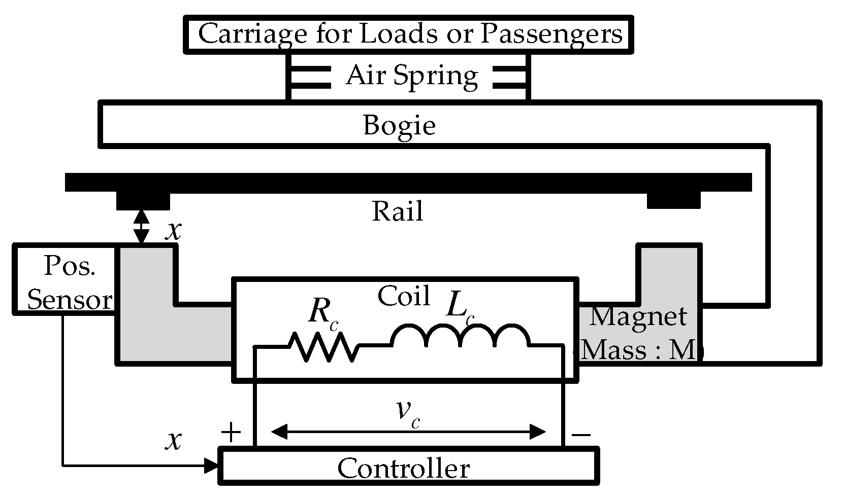
2. Nonlinear Dynamics of MAGLEVs

Figure 1 depicts the hardware configuration of the MAGLEV systems. The coil voltage $v_c$ (in V) regulates its current $i_c$ (in A) triggering the magnetic force ${\displaystyle \frac{K_f}{M}}{\left({\displaystyle \frac{i_c}{x}}\right)}^2$ with coefficients $K_f$ (in N·m²/A²) and M (Magnet mass, in kg), which consecutively results in velocity v (in m/s) and position x (in m) of the MAGLEV systems by the following nonlinear system [4,9]:

$$\begin{array}{ccc}\hfill {\displaystyle \frac{dx}{dt}}& =& v,\hfill \end{array}$$

(1)

$$\begin{array}{ccc}\hfill M{\displaystyle \frac{dv}{dt}}& =& (M+M_L)g-K_f{\left({\displaystyle \frac{i_c}{x}}\right)}^2+f_L,\hfill \end{array}$$

(2)

$$\begin{array}{ccc}\hfill {\displaystyle \frac{d\left(L\left(x\right)i_c\right)}{dt}}& =& -R{i}_c+v_c,\forall t\ge 0,\hfill \end{array}$$

(3)

with the constants g (=$9.8$ m/s²), $M_L$ (in kg), and R (in $\mathsf{\Omega }$) representing the gravity acceleration, load mass, and coil resistance, respectively, and disturbance $f_L$ from the air spring force.

Here, the position x determines the coil inductance $L\left(x\right)$ (in H) such that

$$\begin{array}{c}\hfill L\left(x\right):=L+{\displaystyle \frac{2K_f}{x}}\end{array}$$

(4)

for the base inductance L (in H), which turns the coil current dynamics (3) into the nonlinear system:

$$\begin{array}{c}\hfill L{\displaystyle \frac{d{i}_c}{dt}}=-R{i}_c+v_c+2K_f\left({\displaystyle \frac{v·i_c}{x^2}}\right),\forall t\ge 0,\end{array}$$

(5)

which is used as the basis to design the proposed model-independent filter-based adaptive current tracking controller in Section 3.

3. Structure of Proposed Feedback System

This section consists of two sections; Section 3.1 for the design purpose; and Section 3.2 for the implementation of the proposed solution. In the following sections, the notation $\dot{f}$ represents the time derivative operation ${\displaystyle \frac{df}{dt}}$ for any function f.

3.1. Design Purpose

For any given coil current reference $i_{c,ref}$, this paper purposes for the coil current error defined as ${\tilde{i}}_c:=i_{c,ref}-i_c$ to satisfy the exponential convergence

$$\begin{array}{c}\hfill \underset{t\to \infty }{lim}{\tilde{i}}_c={\tilde{i}}_c^{*}\end{array}$$

(6)

for the desired coil current error ${\tilde{i}}_c^{*}:=i_{c,ref}-i_c^{*}$ derived from the system

$$\begin{array}{c}\hfill {\dot{\tilde{i}}}_c^{*}=-k_c{\tilde{i}}_c^{*},\forall t\ge 0,\end{array}$$

(7)

with the convergence rate $k_c>0$ as the specification of the proposed solution.

Remark 1. 

Supposing ${\dot{i}}_{c,ref}\approx 0$, the desired system (7) yields

$$\begin{array}{c}\hfill {\dot{i}}_c^{*}=k_c(i_{c,ref}-i_c^{*}),\forall t\ge 0,\end{array}$$

with its transfer function from $i_{c,ref}={\mathcal{L}}^{-1}\left\{I_{c,ref}\left(s\right)\right\}$ to $i_c^{*}={\mathcal{L}}^{-1}\left\{I_c^{*}\left(s\right)\right\}$ given by

$$\begin{array}{c}\hfill {\displaystyle \frac{I_c^{*}\left(s\right)}{I_{c,ref}\left(s\right)}}={\displaystyle \frac{k_c}{s+k_c}},\forall s\in \mathbb{C},\end{array}$$

(8)

which indicates that the specification $k_c>0$ can be determined as the bandwidth (e.g., $k_c$ rad/s and ${\displaystyle \frac{k_c}{2\pi }}$ Hz) of the transfer function (8).

3.2. Proposed PI-Type Filter-Based Adaptive Current Tracking Controller

In this subsection, the implementations of the proposed PI-type filter and adaptive control law are presented in Section 3.2.1 and Section 3.2.2, ensuring the design objective (6).

3.2.1. PI-Type Filter for Current Measurement

This paper introduces the filtering objective for the error $e_{i_c}:=i_c-{\widehat{i}}_c$ as the exponential convergence

$$\begin{array}{c}\hfill \underset{t\to \infty }{lim}{e}_{i_c}=e_{i_c}^{*}\end{array}$$

(9)

for $e_{i_c}^{*}:=i_c-{\widehat{i}}_c^{*}$ derived from the desired system

$$\begin{array}{c}\hfill {\dot{e}}_{i_c}^{*}=-k_f{e}_{i_c}^{*},\forall t\ge 0,\end{array}$$

(10)

for given convergence rate $k_f>0$ as the filtering specification.

For the objective (9), the error $e_{i_c}=i_c-{\widehat{i}}_c$ for the filtered current ${\widehat{i}}_c$ defines the proposed PI-type filter given by

$$\begin{array}{c}\hfill {\dot{\widehat{i}}}_c=k_{P,f}{e}_{i_c}+k_{I,f}{\int }_0^t{e}_{i_c}d\tau \end{array}$$

(11)

equipped with the PI gains $k_{P,f}$ and $k_{I,f}$ determined by the design parameter $b_{d_f}>0$ such that

$$\begin{array}{c}\hfill k_{P,f}:=b_{d_f}+k_f\mathrm{and}{k}_{I,f}=b_{d_f}{k}_f\end{array}$$

(12)

for given specification $k_f>0$ driving the desired system (10).

The decomposition $i_c=i_{c,0}+\Delta i_c$ for ${\dot{i}}_{c,0}=0$ (DC) and $\Delta {\dot{i}}_c\ne 0$ (AC) leads to the second-order system for $e_{i_c}=i_c-{\widehat{i}}_c$ along the proposed filter (11) given by

$$\begin{array}{c}\hfill {\ddot{e}}_{i_c}=-k_{P,f}{\dot{e}}_{i_c}-k_{I,f}{e}_{i_c}+f_f\end{array}$$

(13)

where $f_f:=\Delta {\ddot{i}}_c$, $|f_f| \le {\overline{f}}_f$, $\forall t\ge 0$, whose behavior is analyzed in Section 4.

Remark 2. 

The proposed PI-type filter (11) with the nonlinearly structured gain (12) features the two main advantages compared with the conventional low-pass filters (LPFs) and Luenberber observer-type filters:

• (simple structure) The first-order LPF defined as ${\dot{\widehat{i}}}_c=k_f{e}_{i_c}$ leads to the filtering error dynamics as ${\dot{e}}_{i_c}=-k_f{e}_{i_c}+w_{i_c}$ where $w_{i_c}:={\dot{i}}_c$, suffering from the phase delay and magnitude distortion for an high-frequency input $i_c$. The proposed PI-type filter forming the simple structure ensures the improved filtering error dynamics given by

  $$\begin{array}{c}\hfill {\dot{e}}_{i_c}=-k_f{e}_{i_c},\forall t>T,\end{array}$$

  (14)

  for a small $T>0$ through the augmentation of the integral action and order reduction property by the nonlinear structured gain (12).
• (model independence) The proposed filter of (11) with its gain (12) does not necessitate the system model information (unlike the conventional Luenberger observer-type filters), such as (5), while ensures the improved filtering performance (14) by only tuning $b_{d_f}>0$ for given specification $k_f>0$.

and its special gain structure (12) invokes the order reduction property resulting in

$$\begin{array}{c}\hfill {\dot{e}}_{i_c}=-k_f{e}_{i_c},\forall t>T\end{array}$$

for a small $T>0$ by guarantee of the filtering objective (9) under a some choice of $b_{d_f}>0$, which is proved in Section 4.

Remark 3. 

Supposing ${\dot{i}}_c\approx 0$, the desired system (10) yields

$$\begin{array}{c}\hfill {\dot{\widehat{i}}}_c^{*}=k_f(i_c-{\widehat{i}}_c^{*}),\forall t\ge 0,\end{array}$$

with its transfer function from $i_c={\mathcal{L}}^{-1}\left\{I_c\left(s\right)\right\}$ to ${\widehat{i}}_c^{*}={\mathcal{L}}^{-1}\left\{{\widehat{I}}_c^{*}\left(s\right)\right\}$ given by

$$\begin{array}{c}\hfill {\displaystyle \frac{{\widehat{I}}_c^{*}\left(s\right)}{I_c\left(s\right)}}={\displaystyle \frac{k_f}{s+k_f}},\forall s\in \mathbb{C},\end{array}$$

(15)

which indicates that the specification $k_f>0$ can be determined as the bandwidth (e.g., $k_f$ rad/s and ${\displaystyle \frac{k_f}{2\pi }}$ Hz) of the transfer function (10).

3.2.2. Adaptive Current Tracking Control Law

The parameter decomposition $L=L_0+\Delta L$ with the known nominal inductance $L_0$ and its unknown deviation $\Delta L$ yields the open-loop system for ${\tilde{i}}_c=i_{c,ref}-{\widehat{i}}_c$ from (5) as

$$\begin{array}{c}\hfill {\dot{\tilde{i}}}_c=-{\displaystyle \frac{1}{L_0}}{v}_c+d_0+\Delta d+c_f{\dot{e}}_{i_c},\forall t\ge 0,\end{array}$$

(16)

where $c_f:={\displaystyle \frac{L}{L_0}}$, $d:={\displaystyle \frac{1}{L_0}}(-2K_f\left({\displaystyle \frac{v·i_c}{x^2}}\right)+R{i}_c+L{\dot{i}}_{c,ref}-\Delta L{\dot{\tilde{i}}}_c)$, $d=d_0+\Delta d$ for ${\dot{d}}_0=0$ (DC) and $\Delta \dot{d}\ne 0$ (AC), and $|\Delta d|\le \overline{d}$, $\forall t\ge 0$. The proposed P-type adaptive controller stabilizes the open-loop system (16), designed as

$$\begin{array}{c}\hfill v_c=L_0(k_{P,c}{\tilde{i}}_c+{\widehat{d}}_0)\end{array}$$

(17)

with the adaptive rule

$$\begin{array}{c}\hfill {\dot{\widehat{d}}}_0={\gamma }_{ad}{\tilde{i}}_c\end{array}$$

(18)

and feedback and adaptation gains

$$\begin{array}{c}\hfill k_{P,c}:=b_{d_c}+k_c\mathrm{and}{\gamma }_{ad}:=b_{d_c}{k}_c\end{array}$$

(19)

determined by the design parameter $b_{d_c}>0$ for given specification $k_c>0$ in (7).

After substituting the proposed adaptive current controller of (17) and (18) to the open-loop system (16) gives the closed-loop dynamics:

$$\begin{array}{ccc}\hfill {\dot{\tilde{i}}}_c& =& -k_{P,c}{\tilde{i}}_c+{\tilde{d}}_0+\Delta d+c_f{\dot{e}}_{i_c},\hfill \end{array}$$

(20)

$$\begin{array}{ccc}\hfill {\dot{\tilde{d}}}_0& =& -{\gamma }_{ad}{\tilde{i}}_c,\hfill \end{array}$$

(21)

where ${\tilde{d}}_0:=d_0-{\widehat{d}}_0$, $f_c:=\Delta \dot{d}$, $|f_c|\le {\overline{f}}_c$, $\forall t\ge 0$, whose behavior is analyzed in Section 4. Figure 2 represents the feedback system structure of the proposed technique.

4. Closed-Loop Analysis Results

This section purposes to present closed-loop analysis results, including the guarantee of the control objective (6) through further analysis of the closed-loop filtering and current dynamics of (13) and (A7) with their special gain structures (12) and (19) invoking the order reduction. Appendix A provides the proofs of the following lemmas and theorems.

4.1. Analysis of Filtering Loop

The filter gain determined by the special structure of (12) cuts the order of the filtering error dynamics (13) to 1 by the order reduction, which is addressed by Lemma 1 (refer to Appendix A for the proof).

Lemma 1. 

The proposed PI-type filter of (11) equipped with the gain (12) drives the filtering error $e_{i_c}=i_c-{\widehat{i}}_c$ governed by the system

$$\begin{array}{c}\hfill {\dot{e}}_{i_c}=-k_f{e}_{i_c}+y_f\end{array}$$

(22)

perturbed by $x_f$ satisfying

$$\begin{array}{c}\hfill {\dot{y}}_f=-b_{d_f}{y}_f+f_f,\forall t\ge 0.\end{array}$$

(23)

Lemma 2 derives a feasible tuning range for $b_{d_f}>0$ to ensure the exponential convergence (10) by the proposed PI-type filter based on the results (22) and (23) obtained by Lemma 1 (refer to Appendix A for the proof).

Lemma 2. 

The proposed PI-type filter of (11) equipped with the gain (12) guarantees

$$\begin{array}{c}\hfill \underset{t\to \infty }{lim}{e}_{i_c}=e_{i_c}^{*}\end{array}$$

(24)

exponentially for any $b_{d_f}>0$ satisfying ${\displaystyle \frac{2{\overline{f}}_f}{b_{d_f}}}\approx 0$ where the signal $e_{i_c}^{*}$ satisfies the system (10).

Remark 4. 

Lemma 2 proves the statement of Remark 2 by specifying a feasible tuning range for $b_{d_f}>0$ for given specification $k_f>0$, which eventually allows to use

$$\begin{array}{c}\hfill {\dot{e}}_{i_c}=-k_f{e}_{i_c}\end{array}$$

(25)

for the remaining analysis of this section.

4.2. Analysis of Control Loop

The control gain determined by the special structure of (19) cuts the order of the closed-loop dynamics of (20) and (21) to 1 by the order reduction, which is addressed by Lemma 3 (refer to Appendix A for the proof).

Lemma 3. 

The proposed adaptive controller of (17) equipped with the gain (19) drives the filtering error ${\tilde{i}}_c=i_{c,ref}-{\widehat{i}}_c$ governed by the system

$$\begin{array}{c}\hfill {\dot{\tilde{i}}}_c=-k_c{\tilde{i}}_c+{\mathit{𝟭}}^T{\mathit{y}}_c\end{array}$$

(26)

perturbed by ${\mathit{x}}_c$ satisfying

$$\begin{array}{c}\hfill {\dot{\mathit{y}}}_c=-b_{d_c}{\mathit{y}}_c+\mathit{b}{e}_{i_c}+{\mathit{e}}_2{f}_c,\forall t\ge 0,\end{array}$$

(27)

for some $\mathit{b}\in {\mathbb{R}}^2$ where 1$:=\left[\begin{array}{c}1\\ 1\end{array}\right]$.

Theorem 1 provides the proof to guarantee the control objective (6) by deriving a feasible tuning range for $b_{d_c}>0$ on the basis of the results (25), (26) and (27) obtained by Lemmas 1–3 (refer to Appendix A for the proof).

Theorem 1. 

The proposed adaptive controller of (17) equipped with the gain (19) guarantees the control objective (6) for any $b_{d_c}>0$ satisfying ${\displaystyle \frac{2{\overline{f}}_c}{b_{d_c}}}\approx 0$ (e.g., establishment of the exponential convergence ${lim}_{t\to \infty }{\tilde{i}}_c={\tilde{i}}_c^{*}$).

Remark 5. 

The results of Lemma 2 and Theorem 1 derive a tuning direction of the design parameters for the proposed PI-type filter and adaptive current controller given by

• (PI-type filter by Lemma 2)

  1.

  Determine the desired filtering performance as ${\dot{e}}_{i_c}^{*}=-k_f{e}_{i_c}^{*}$ for some $k_f>0$.

  2.

  Increase $b_{d_f}>10$ by observing $|e_{i_c}^{*}-e_{i_c}|\approx 0$, $\forall t\ge 0$.

• (Adaptive current controller by Theorem 1)

  1.

  Determine the desired coil current control performance ${\dot{\tilde{i}}}_c^{*}=-k_c{\tilde{i}}_c^{*}$ for some $k_c>0$.

  2.

  Increase $b_{d_c}>10$ by observing $|{\tilde{i}}_c^{*}-{\tilde{i}}_c|\approx 0$, $\forall t\ge 0$.

These iterations result in the tuned values for the design parameters of the proposed technique used in Section 5.

5. Simulations

This section numerically evaluates the performance of the proposed feedback system as the subsystem of the MAGLEV positioning technique in [25] using MATLAB/Simulink (ver. 2017b), whose implementation is depicted in Figure 3. Here, the nonlinear differential equations of (1), (2), and (3) realized the motions of the MAGLEV system with the coefficients $R=4.4$, and $L=908\times {10}^3$, $M=725$, $M_L=300$, and $K_f=5.45\times {10}^{-3}$ through the ordinary differential equations (ODE) solver of the Simulink. The combination of C-programming and S-function provided by Simulink constructed the filter and controller as the internal interrupt service (ISR) with the period of 1 ms using the nominal inductance $L_0=1.3L$. The recent multi-loop position regulator in [25] yielded the coil current reference $i_{c,ref}$ to stabilize the rail position x to its reference $x_{ref}$ for given bandwidth ${\omega }_p=2\pi f_p$ rad/s with $f_p=0.5$ Hz such that

• (P control for velocity reference)

  $$\begin{array}{c}\hfill v_{ref}={\omega }_p(x_{ref}-x),\end{array}$$

  (28)
• (PI control for acceleration reference)

  $$\begin{array}{c}\hfill a_{ref}=k_{P,a}(v_{ref}-v)+k_{I,a}{\int }_0^t(v_{ref}-v)d\tau ,\end{array}$$

  (29)
• (Current reference calculation)

$$\begin{array}{c}\hfill i_{c,ref}=\sqrt{{\displaystyle \frac{M{x}^2}{K_f}}(-a_{ref}+g)},\end{array}$$

(30)

equipped with a well-tuned PI gains

$$\begin{array}{c}\hfill k_{P,a}=0.5\mathrm{and}{k}_{I,a}=2\end{array}$$

to ensure the exponential convergence ${lim}_{t\to \infty }x=x^{*}$ for ${\dot{x}}^{*}={\omega }_{xc}(x_{ref}-x^{*})$, $\forall t\ge 0$. Figure 3 shows the resultant feedback system structure for the performance evaluation.

The proposed filter and control law was tuned as follows:

• (filter) $b_{d_f}=1000$ for ${\dot{e}}_{i_c}\approx -k_f{e}_{i_c}$ with $k_f=2\pi 10$ and
• (controller) $b_{d_c}=2000$ for ${\dot{\tilde{i}}}_c\approx -k_c{\tilde{i}}_c$ with $k_c=2\pi 6$.

The active damping (AD) controller in [25], given by $i_{c,ref}=L_0\left(-b_{d,AD}{i}_c+k_c(i_{c,ref}-i_c)+b_{d,AD}{k}_c{\int }_0^t(i_{c,ref}-i_c)d\tau \right)$, was adopted for comparison study including the tuned value $b_{d,AD}=5000$ for the same bandwidth $k_c=2\pi 6$ rad/s with the proposed controller.

5.1. Rail Position Tracking Performance Evaluation

This stage applied a piece-wise constant position reference with its initial value $x_{ref}=0.01$ m, which is sequentially increased to $0.03$ and $0.05$ and restored to $0.01$ m. For this position reference, this simulation was conducted for three closed-loop bandwidths $f_p=0.5$, $1.0$, and $1.7$ Hz to evaluate the closed-loop robustness for the proposed adaptive current controller, compared with the AD controller. Figure 4 highlights the main merit of the proposed controller successfully stabilizing the high-speed operation mode at $f_p=1.7$ Hz, unlike the AD controller. The combination of adaptation and order reduction mechanisms led to this advantage of the proposed controller. Figure 5 presents the resultant rail speed responses for three closed-loop bandwidths, indicating the successful rail velocity stabilization for the high-speed operation mode at $f_p=1.7$ Hz by the proposed controller. Figure 6 shows that the proposed controller forced the coil current to track its reference without errors, as guaranteed by Theorem 1, but the AD controller suffered from tracking errors during the transient periods. The left side of Figure 7 confirmed the filtering error stabilization as the result of Lemma 2, which contributes to maintaining the desired feedback system performances. The corresponding adaptation results were shown on the right side of Figure 7.

5.2. Rail Position Stabilization Performance Evaluation

For fixed closed-loop bandwidth $f_p=0.5$ Hz, this stage evaluates the rail position stabilization performance for sudden load variations by introducing the three load mass changing scenarios such that $M_L$ is increased from 300 to $400/800/1300$, and restored to 300 kg sequentially. Figure 8 also points out the practical advantage of the proposed controller securing the successful rail position stabilization despite the sudden load mass change from $M_L=1300$ to 300 kg, unlike the AD controller. This improved robustness was obtained by the systematical feedback system design process considering the nonlinearity and modeling errors, conducted in Section 3 and Section 4. Figure A1 shows the improved over/undershoot reduction and stabilization capability of the rail velocity by the proposed controller. Figure A2 presents the reference tracking results of the coil current, indicating considerably lowered tracking errors by the proposed controller, compared with the AD controller, due to the result of Theorem 1.

5.3. Numerical Performance Comparison Results

The table in Figure A3 numerically compares the closed-loop performances obtained by the proposed and AD controllers based on the evaluation function defined as $f_{eval}:=\sqrt{{\int }_0^{\infty }|x_{ref}{-x|}^2+v^2+{|i_{c,ref}-i_c|}^{2}dt}$. As shown in this table, the proposed controller improved the closed-loop performance by $25\%$ at least over the simulation scenarios in Section 5.1 and Section 5.2, which corresponds to a significant improvement for the actual applications with the simple implementation in Figure 2.

5.4. Computational Time Consumption Comparison Results

This evaluation finalizes this section by presenting the computational time consumption comparison results in Figure A4, which was conducted using a 32-bit digital signal processor (DSP28377 manufactured by Texas Instruments (Dallas, TX, USA)), compared with the AD controller. The time consumption for each controller was measured for $2\times {10}^3$ times using the random current references satisfying $i_{c,ref}\in [1,80]$. Figure A4 tabulates the resultant averaged values, showing the feasibility of the proposed controller for the industrial power electronic-based actual implementations.

6. Conclusions

This paper designed an advanced adaptive current tracking controller to secure an improved positioning performance of the MAGLEV systems subject to modeling errors, load variations, and simplicity for actual implementations. The proposed technique included the model-independent PI-type filter to improve the closed-loop accuracy in the presence of current measurement noises, constructing the simple P-type adaptive current control law. To highlight the academic contributions, the proofs for the closed-loop performance and stability were provided, whose practical improvements were validated by the numerical simulations using MATLAB/Simulink. An expansion for the case of six degrees of freedom will be considered with a combination of the outer and middle loop controls in future studies, including experimental verification.

References

1. Li, A.; Cui, H.; Guan, Y.; Deng, J.; Zhang, Y.; Deng, W. Study on Aerodynamic Drag Reduction by Plasma Jets for 600 km/h Vacuum Tube Train Sets. Machines 2023, 11, 1078. [Google Scholar] [CrossRef]
2. Wang, Y.; Gao, H. Simulation Analysis and Online Monitoring of Suspension Frame of Maglev Train. Machines 2023, 11, 607. [Google Scholar] [CrossRef]
3. Wang, Z.; Li, X.; Xie, Y.; Long, Z. MAGLEV Train Signal Processing Architecture Based on Nonlinear Discrete Tracking Differentiator. Sensors 2018, 18, 1697. [Google Scholar] [CrossRef] [PubMed]
4. Nguyen, C.X.; Pham, T.D.; Lukynov, A.D.; Tran, P.C.; Truong, Q.D. Design embedded control system based controller of the quasi time optimization approach for a magnetic levitation system. In IOP Conference Series: Materials Science and Engineering; IOP Publishing: Bristol, UK, 2021. [Google Scholar]
5. Zhang, L.; Campbell, S.; Huang, L. Nonlinear analysis of a MAGLEV system with time-delayed feedback control. Phys. D Nonlinear Phenom. 2012, 240, 1761–1770. [Google Scholar] [CrossRef]
6. Santos, M.; Ferreira, J.; Simoes, J.; Pascoal, R.; Torrao, J.; Xue, X.; Furlani, E. Magnetic levitation-based electromagnetic energy harvesting: A semi-analytical non-linear model for energy transduction. Sci. Rep. 2016, 6, 18579. [Google Scholar]
7. Zhang, Z.; Zhang, L. Hopf bifurcation of time-delayed feedback control for MAGLEV system with flexible guideway. Appl. Math. Comput. 2013, 219, 6106–6112. [Google Scholar] [CrossRef]
8. Lee, H.W.; Kim, K.C.; Lee, J. Review of MAGLEV train technologies. IEEE Trans. Magn. 2006, 42, 1917–1925. [Google Scholar]
9. Zhang, Z.; Li, X. Real-Time Adaptive Control of a Magnetic Levitation System with a Large Range of Load Disturbance. Sensors 2018, 18, 1512. [Google Scholar] [CrossRef]
10. Kim, C.H. Robust Control of Magnetic Levitation Systems Considering Disturbance Force by LSM Propulsion Systems. IEEE Trans. Magn. 2017, 53, 8300805. [Google Scholar] [CrossRef]
11. Wai, R.J.; Lee, J.D.; Chuang, K.L. Real-time PID control strategy for MAGLEV transportation system via particle swarm optimization. IEEE Trans. Ind. Electron. 2011, 58, 629–646. [Google Scholar] [CrossRef]
12. Shamma, J.S.; Athans, M. Analysis of gain scheduled control of nonlinear plants. IEEE Trans. Autom. Control 2002, 35, 898–907. [Google Scholar] [CrossRef]
13. Olalla, C.; Leyva, R.; Queinnec, I.; Maksimovic, D. Robust Gain-Scheduled Control of Switched-Mode DC-DC Converters. IEEE Trans. Power Electron. 2012, 27, 3006–3019. [Google Scholar] [CrossRef]
14. Yang, J.; Zolotas, A.; Chen, W.H.; Michail, K.; Li, S. Robust control of nonlinear MAGLEV suspension system with mismatched uncertainties via DOBC approach. ISA Trans. 2011, 50, 389–396. [Google Scholar] [CrossRef] [PubMed]
15. Tian, Z.; Zhong, Q.C.; Ren, B.; Yuan, J. Stabilisability analysis and design of UDE-based robust control. IET Control Theory Appl. 2019, 13, 1445–1453. [Google Scholar] [CrossRef]
16. Huang, G.; Huang, H.; Zhai, Y.; Tang, G.; Zhang, L.; Gao, X.; Huang, Y.; Ge, G. Multi-Sensor Fusion for Wheel-Inertial-Visual Systems Using a Fuzzification-Assisted Iterated Error State Kalman Filter. Sensors 2024, 24, 7619. [Google Scholar] [CrossRef]
17. Liang, Z.; Fan, S.; Feng, J.; Yuan, P.; Xu, J.; Wang, X.; Wang, D. An Enhanced Adaptive Ensemble Kalman Filter for Autonomous Underwater Vehicle Integrated Navigation. Drones 2024, 8, 711. [Google Scholar] [CrossRef]
18. Wu, J.; Li, Y.; Sun, Q.; Zhu, Y.; Xing, J.; Zhang, L. Joint Battery State of Charge Estimation Method Based on a Fractional-Order Model with an Improved Unscented Kalman Filter and Extended Kalman Filter for Full Parameter Updating. Fractal Fract. 2023, 8, 695. [Google Scholar] [CrossRef]
19. Wai, R.J.; Lee, J.D. Backstepping-based levitation control design for linear magnetic levitation rail system. IET Control Theory Appl. 2008, 2, 72–86. [Google Scholar] [CrossRef]
20. Kaloust, J.; Ham, C.; Siehling, J.; Jongekryg, E. Nonlinear robust control design for levitation and propulsion of a MAGLEV system. IET Control Theory Appl. 2004, 151, 460–464. [Google Scholar] [CrossRef]
21. Sadek, U.; Sarja, A.; Chowdhury, A.; Cko, R.S. Improved adaptive fuzzy backstepping control of a magnetic levitation system based on symbiotic organism search. Appl. Soft Comput. 2017, 56, 19–33. [Google Scholar] [CrossRef]
22. Sun, Y.; Li, W.; Xu, J.; Qiang, H.; Chen, C. Nonlinear dynamic modeling and fuzzy sliding-mode controlling of electromagnetic levitation system of low-speed MAGLEV train. J. Vibroeng. 2017, 19, 328–342. [Google Scholar] [CrossRef]
23. Wai, R.J.; Lee, J.D. Robust Levitation Control for Linear MAGLEV Rail System Using Fuzzy Neural Network. IEEE Trans. Control Syst. Technol. 2009, 17, 4–14. [Google Scholar]
24. Xu, J.; Du, Y.; Chen, Y.H.; Guo, H. Adaptive robust constrained state control for non-linear MAGLEV vehicle with guaranteed bounded airgap. IET Control Theory Appl. 2018, 12, 1573–1583. [Google Scholar] [CrossRef]
25. Kim, S.K. Nonlinear Position Stabilizing Control with Active Damping Injection Technique for Magnetic Levitation Systems. Electronics 2019, 8, 221. [Google Scholar] [CrossRef]
26. Kim, S.K.; Ahn, C.K. Variable Cut-Off Frequency Algorithm-Based Nonlinear Position Controller for Magnetic Levitation System Applications. IEEE Syst. Man Cybern. Syst. 2021, 51, 4599–4605. [Google Scholar] [CrossRef]
Figure 1. Hardware configuration of MAGLEV systems.
Machines 12 00880 g001
Figure 2. Feedback system structure of proposed adaptive current tracking controller.
Machines 12 00880 g002
Figure 3. Structure of proposed feedback system.
Machines 12 00880 g003
Figure 4. Position response comparison for reference tracking mode with closed-loop bandwidths f p = 0.5 , 1.0 , and 1.7 Hz.
Machines 12 00880 g004
Figure 5. Velocity response comparison for reference tracking mode with closed-loop bandwidths f p = 0.5 , 1.0 , and 1.7 Hz.
Machines 12 00880 g005
Figure 6. Coil current response comparison for reference tracking mode with closed-loop bandwidths f p = 0.5 , 1.0 , and 1.7 Hz.
Machines 12 00880 g006
Figure 7. Filtering error and adaptation responsts for reference tracking mode with closed-loop bandwidths f p = 0.5 , 1.0 , and 1.7 Hz.
Machines 12 00880 g007
Figure 8. Position response comparison for reference regulation mode with load variations M L : 300 400 / 800 / 1300 300 kg.
Machines 12 00880 g008
Disclaimer/Publisher’s Note: The statements, opinions and data contained in all publications are solely those of the individual author(s) and contributor(s) and not of MDPI and/or the editor(s). MDPI and/or the editor(s) disclaim responsibility for any injury to people or property resulting from any ideas, methods, instructions or products referred to in the content.