Comparing Skill Transfer Between Full Demonstrations and Segmented Sub-Tasks for Neural Dynamic Motion Primitives

Abstract

Programming by demonstration has shown potential in reducing the technical barriers to teaching complex skills to robots. Dynamic motion primitives (DMPs) are an efficient method of learning trajectories from individual demonstrations using second-order dynamic equations. They can be expanded using neural networks to learn longer and more complex skills. However, the length and complexity of a skill may come with trade-offs in terms of accuracy, the time required by experts, and task flexibility. This paper compares neural DMPs that learn from a full demonstration to those that learn from simpler sub-tasks for a pouring scenario in a framework that requires few demonstrations. While both methods were successful in completing the task, we find that the models trained using sub-tasks are more accurate and have more task flexibility but can require a larger investment from the human expert.

1. Introduction

Robotic manipulators have the potential for many benefits in our society. They have been applied in many settings to increase productivity by automating repetitive tasks, improving efficiency, increasing safety, and enhancing reliability [1,2]. Recently, there has been increased research into using robotic manipulators in complex environments with high degrees of uncertainty and requiring a high level of expertise, such as in medical applications [3,4,5] and maintenance settings [6,7]. These new applications of robotics increase the need for programming interfaces that can be quickly customized and programmed to complete different tasks to suit the needs of the expery without relying on programming and robotics expertise.

Learning from demonstration, also known as behavioral cloning or imitation learning, is a supervised machine learning technique designed to be a more intuitive and flexible method of robot programming [8] that can also be used to transfer skills from users who are not experts in programming or robotics. Instead of designing specific control architectures, learning from demonstration frameworks allows users who are experts in the desired tasks to interact directly with robots to transfer skills. Demonstrations performed by one or more experts are collected by the system and are used to generate a model of how the task should be completed. This model can then be used to complete the same task and potentially generalize to variations in the task or environment. The ability to learn from demonstration frameworks to be utilized by non-programmers allows them to be an important step toward the flexible programming of robotic manipulators.

Dynamic motion primitives (DMPs) are a learning-from-demonstration method and represent trajectories using second-order dynamic systems [9]. They have several characteristics that make them attractive for learning from demonstrations in robotics, including stability guarantees, learning from a single demonstration, and the capability for generalization. They are a flexible framework that can be formulated in different task spaces, such as joint space or Cartesian space, making them suitable for various purposes. They can also learn from a single demonstration, which can reduce the time and resources required to collect training data.

DMPs can be combined with neural networks to extend the functionality of DMPs by forming what is known as neural DMPs [10]. This allows for further generalization of DMPs through training from multiple demonstrations. However, this can come at the cost of requiring more investment into the demonstration collection process, which can be time-consuming and expensive, as experts are required for very specialized tasks. Additionally, leveraging the function approximation capabilities of neural networks, neural DMPs can increase the complexity and duration of tasks that can be modeled. This presents the option of learning from a full demonstration instead of dividing it into sub-tasks, eliminating the need for experts to process and divide the demonstrations once they have been collected.

1.1. Motivation

A common approach used when programming robots for tasks, including for learning from demonstration, is to break down tasks into sub-tasks. Segmenting tasks in this manner has several advantages, such as reducing the complexity where modeling is required and some flexibility to combine motions in different orders, and it can be very effective in controlled and well-structured environments such as manufacturing [8]. However, decomposing tasks can introduce challenges in current DMP-based controllers, such as requiring a carefully designed framework to combine the sub-tasks, which may need to be modified for changes in the task and require a larger time investment into collecting and processing demonstrations. As such, the systems are still reliant on individuals with robotics and programming expertise, particularly when the system may need to be retrained quickly and often for specific tasks such as in medical and maintenance applications. This limits their usefulness and customization to the user’s specific needs. As such, this paper aims to compare the use of DMPs when using demonstrations of complete tasks to DMPs using demonstrations of individual sub-tasks, with the goal of reducing the necessary technical expertise and resource investment required for programming from demonstration.

Decreasing the reliance on expert programmers and roboticists when teaching new skills is one step toward reducing the barrier to entry for robotic systems for widespread use. Leveraging neural DMPs is one avenue of learning sequences of tasks from complete demonstrations to create a programming interface for robot manipulators. This will allow experts to provide demonstrations in applications such as leg positioning during rehabilitation, or machinery repairing sequences, which can then be transferred to a robot manipulator without modifying the underlying framework. However, while this can result in a faster transfer of skills, it may come with trade-offs when compared to a segmented approach. Comparisons between learning from full and segmented approaches have not been thoroughly addressed in current research.

Collecting a sufficient number of high-quality demonstrations is another challenge to be overcome to increase the prevalence of learning from demonstration for robotics. The lack of available demonstrations is more prevalent in tasks that occur infrequently or that may occur in dangerous locations, such as deep sea welding or maintenance tasks in outer space. The number of training samples varies between different learning methods, meaning methods that are effective with few samples can reduce the time and effort required during data collection. Synthetically generated data have also been used to train models for certain tasks [11], although this is limited by the ability to simulate the completion of the objective and can often negate the modeling benefits obtained from learning by demonstration. Data augmentation can also be used to circumvent this challenge by increasing both the number and variety of samples in the datasets [12].

1.2. Contributions

In this paper, we demonstrate the ability of neural DMPs to learn a skill with few human demonstrations and compare it to a model that has learned from demonstrations split into sub-tasks, as traditionally performed in DMPs. The trade-offs in accuracy, along with other important factors such as the amount of input required from human experts and the potential task flexibility capabilities between the two models, are then analyzed. To assess these trade-offs quantitatively and qualitatively, we utilize neural DMPs with a simple yet nontrivial task—pouring water into a glass. We perform the learning both from a full demonstration and by segmenting the demonstration into sub-tasks; then, we compare them in terms of the required human input, accuracy, and potential for flexibility. The main contributions are as follows:

• We demonstrate that neural DMPs can be used to learn a task made up of multiple sub-tasks from full demonstrations (unsegmented).
• We compare the accuracy of neural DMP models trained using full demonstrations to those trained using simpler sub-tasks and examine key trade-offs between the models trained using full demonstrations to those trained using simpler sub-tasks.
• We demonstrate the ability of neural DMP models to learn from a dataset that requires minimal human demonstrations to generalize for a pouring task.

The remainder of this paper is structured as follows. Section 2 explores the related works and knowledge gaps. Next, Section 3 describes the theoretical foundation and training methods for DMPs. Section 4 outlines the process used to collect demonstrations to form the dataset, and Section 5 presents the results after training the models and implementing them on the robot. Section 6 discusses the results, and Section 7 summarizes the conclusions and presents potential future directions.

2. Related Works

Dynamic motion primitives (DMPs) are a versatile method of learning from demonstration that represents trajectories using second-order dynamical systems [13]. They are composed of a set of basis functions, learned weights, and attractor dynamics, allowing a model to be trained from a single demonstration. DMPs have been formulated for both joint space and Cartesian space and have been augmented to incorporate environmental feedback and external stimuli [14]. They are a proven method of effective learning from demonstrations, but they can have certain drawbacks, such as only learning from a single demonstration, which can limit the ability to generalize.

While traditional DMPs are formulated for joint or Cartesian position control, formulations for both quaternion [15] and rotation-matrix-based orientations [16], as well as combined positions and orientation for Cartesian spaces [17,18], have been developed. Joint-space DMPs tend to be popular when recording robot joint states during demonstrations, such as for kinesthetic teaching or teleoperation-based interfaces [19]. While joint-space DMPs can be used with passive observations, this often requires overcoming the correspondence problem or mapping human joints to robot joint space (retargeting), which can be challenging due to different kinesthetic makeups and redundancies [20]. As such, position, orientation, and Cartesian space DMPs are popular when humans perform the demonstrations independently of the robot. Additionally, DMPs can represent point-to-point motions or periodic motions or even have goals with a non-zero velocity [14]. While each method is rooted in similar theoretical formulations, selecting the correct DMP for a particular task representation is crucial. In this paper, demonstrations were collected using passive observation; therefore, Cartesian DMPs were selected to control the position and orientation of the end effector in completing the task. Point-to-point DMPs were selected as the demonstrations, and segmented demonstrations had zero starting and ending velocities and accelerations.

While modifications to adapt to uncertain environments serve to improve the robustness of DMPs, applying them to more complex tasks requires additional strategies. Integrating via-points into the DMP formulation allows further control when specific and known points in a trajectory are critical for task execution. These can be incorporated based on knowledge of the desired trajectory [21] and have also been implemented at run time for dynamic obstacle avoidance or changing environmental factors [22]. However, it should be noted that even with via points, the amount to which a motion primitive can be adapted to meet the constrained point in the trajectory is limited [21]. Further control over tasks with multiple distinct steps can be obtained by training and executing multiple consecutive DMPs, which is a common strategy [17,23]. While the segmentation can be performed autonomously, typically using zero velocity crossing [24], this can require human oversight, which can become more difficult to obtain when highly trained experts are required. When combined with a higher-level planner that selects from a library of primitives [25,26], this can provide further task generalization and adaptability. However, the system is still limited to the primitives that it has and requires the processing of environmental data to select the correct primitive.

Adding more control to DMPs through via points and DMP chaining introduces additional control for tasks but requires more effort to implement and train. Sidiropoulos and Doulgeri [22] utilize via points in real time, but this requires monitoring the environment for obstacles or changes in the environment that are known to impact the current task. Similarly, static via points require known points critical to the trajectory, which need to be selected in some manner [21]. While DMP chaining can be performed through velocity zero-crossing [24], it may still require human oversight to correct segmentation or when specific augmentations are required. These techniques reintroduce task knowledge handcrafted human inputs, albeit to a lesser extent, which are preferably to be avoided when using learning from demonstration.

A key feature of DMPs is that they learn from a single demonstration, which provides both advantages and disadvantages. Data-driven models that do not require large amounts of data are useful in machine learning to reduce the time and effort required to collect datasets. In robotics, particularly for techniques that collect demonstrations from the robot, the ability to learn from small datasets is even more advantageous as it can reduce the physical wear on the system. However, it is often desirable to learn using multiple demonstrations to integrate characteristics of different experts and generalize over tasks. As such, different methods have been explored to allow DMPs to learn from multiple demonstrations.

A variety of techniques have been used to train DMPs from multiple demonstrations. Early methods have explored adding an additional term to the DMP known as the style parameter [27]. Other approaches focus on training multiple DMPs and finding locally optimal solutions through quadratic optimization [28,29]; however, these methods tend not to scale efficiently, as training and storing DMPs for each demonstration is required. A combination of Gaussian mixture models (GMMs) and Gaussian mixture regression (GMR) [30] has also been used to train DMPs for multiple demonstrations, including demonstrations of correct and incorrect behaviors [31]. Using DMPs along with a learned cost function in model predictive control (MPC) has also been used [32] and has been shown to scale more efficiently with the number of demonstrations. Linear regression has also been used to learn unique weights throughout a task space based on multiple demonstrations [33].

Currently, neural networks are a popular method being used to generalize over multiple demonstrations [10]. Often referred to as neural DMPs, this technique uses a neural network to approximate the weights of a DMP using environmental factors as inputs and using trajectory representation characteristics of the DMPs. End-to-end policies, which take images of the environments, have been developed to avoid hand-crafted features [11]. Neural DMPs for orientation are less common but have been investigated [18], and the weights are learned by comparing the forcing functions. Different types of neural networks, including traditional networks and recurrent neural networks (RNNs) [34], as well as convolutional neural networks (CNNs) [35], have been used.

Different loss functions have been used while learning the weights for DMPs from neural networks. When this is performed, it must be differentiable with respect to the desired outputs, generally the weights and desired goal position, to ensure that back-propagation can occur in the network. The forcing functions from the learned model and the demonstrations have been used to generate the loss function and neural network weight updates for both position and orientation representations [18]. Another method computes the loss function for training a position of neural DMP by comparing the output trajectory to the demonstration, as opposed to comparing the weights, which do not have a physical meaning [36], and is found to increase the performance of the networks. Auto-encoders have also been used to learn latent space representations of tasks for motion generation [37], so they are also able to compare reconstructed trajectories to demonstrations. For this system, the loss function for the position was determined by comparing the demonstration trajectory and the modeled trajectory as in [36], while the orientation loss function compared the learned and modeled forcing function as in [18].

While the use of DMPs has been common in robotics, limited research has explored the use of neural DMPs to learn longer sequences of tasks from a single demonstration. This paper aims to fill this gap by first developing a neural DMP model trained from a single demonstration and then comparing it to one trained from segmented demonstrations. The comparison is performed in terms of task precision, the additional time required to process demonstrations, and the potential for flexibility within the framework.

3. Methodology

3.1. Dynamic Motion Primitives

Equations (1) and (2) show the transformation system and auxiliary variable for the classical formulation for DMPs [14]. Together, these form a second-order differential equation that defines the shape of a trajectory while ensuring convergence to the goal.

$$\tau \dot{z}={\alpha }_z({\beta }_z(g-y)-z)+f\left(x\right)$$

(1)

$$\tau \dot{y}=z,$$

(2)

where $\tau$ is the time scaling factor, g is the final goal point, y is the trajectory variable, and z is the auxiliary variable as formulated in [14]. The variables ${\alpha }_z$ and ${\beta }_z$ are hyper-parameters that create a critically damped system when ${\alpha }_z=4{\beta }_z$. The variable x is the canonical variable that makes the transformation system independent of time through the canonical system given by Equation (3). This allows for easier deployment, analysis, and control over the properties of the DMP. The forcing term $f\left(x\right)$ defines the shape of the trajectory between the initial position and the goal through a set of weights learned from a demonstration and a corresponding set of basis functions, and its formulation is shown in Equation (4).

$$\tau \dot{x}=-{\alpha }_{x}x,$$

(3)

The canonical system shown in Equation (3) is an exponential function described by the parameter ${\alpha }_x$. Equation (4) shows the forcing term.

$$f\left(x\right)={\displaystyle \frac{{\sum }_{i=1}^N{\omega }_i{\mathit{\psi }}_i\left(x\right)}{{\sum }_{i=1}^N{\mathit{\psi }}_i\left(x\right)}}x$$

(4)

It is composed of a set of Gaussian basis functions $\mathit{\psi }\left(x\right)$ and learned weights ${\omega }_i$, where N is the number of basis functions used. The basis functions are given by

$${\mathit{\psi }}_i\left(x\right)=exp(-h_i{(x-c_i)}^2),$$

(5)

where each $c_i$ represents the center of a Gaussian basis function and $h_i$ controls its width. When $\tau$ is set to the duration of the demonstration, and N is known, the centers of the basis functions can be distributed according to the following equations.

$$c_i=\exp \left({\displaystyle \frac{{\alpha }_x(i-1)}{N-1}}\right)$$

(6)

$$h_i={\displaystyle \frac{1}{{(c_{i+1}-c_i)}^2}},h_N=h_{N-1}$$

(7)

To represent trajectories in multiple dimensions, multiple DMPs can be used and synchronized through a common canonical system. The weights are typically learned through a Locally Weighted Regression (LWR) from a single demonstration [38].

3.2. Orientation Dynamic Motion Primitives

The quaternion formulation for orientation DMPs [37] is used in this framework and was selected to have a method of representing orientations without singularities. Additionally, it only uses four parameters, as opposed to the nine required for rotation matrices [16]. The formulation is briefly described here, with a quaternion represented by a vector $\mathit{q}=w+\mathit{u}\in {\mathbb{S}}^3$, where w is the real component and $\mathit{u}\in {\mathbb{R}}^3$ are the imaginary components. Equations (8) and (9) show the transformational system for the quaternion DMP.

$$\tau \dot{\mathit{\eta }}={\alpha }_z({\beta }_{z}2{\mathrm{Log}}^q(\mathit{g}\ast \overline{\mathit{q}})-\mathit{\eta })+{\mathit{f}}_q\left(x\right)$$

(8)

$$\tau \dot{\mathit{q}}={\displaystyle \frac{1}{2}}\mathit{\eta }\ast \mathit{q}$$

(9)

Here, $\dot{\mathit{\eta }}\in {\mathbb{R}}^3$ represents the scaled angular velocity, $\dot{\mathit{q}}\in {\mathbb{R}}^4$ is the quaternion derivative, $\overline{\mathit{q}}$ is the quaternion conjugate, and ${\alpha }_z$ and ${\beta }_z$ are parameters to tune the DMP. The ∗ operation represents a quaternion multiplication, and the quaternion logarithm ${\mathrm{Log}}^q(·)$ is shown in Equation (10), in which $\left|\right|·\left|\right|$ is the $l2$ norm of a vector.

$${\mathrm{Log}}^q\left(\mathit{q}\right)=\left\{\begin{array}{cc}\arccos \left(w\right){\displaystyle \frac{\mathit{u}}{\left|\right|\mathit{u}\left|\right|}},\hfill & \mathit{u}\ne \mathbf{0}\hfill \\ {\left[000\right]}^T,\hfill & otherwise\hfill \end{array}\right.$$

(10)

The quaternion DMP uses the same canonical function, forcing term, and basis function center and width equations shown in Equations (3), (4), (6) and (7), respectively. As with classical DMPs, LWR is often used to learn the weights of the forcing term.

3.3. Neural Dynamic Motion Primitives

Neural networks that use the Euclidean distance between the trajectory and the predicted trajectory have been shown have a higher performance than with the loss function based on forcing terms [36]. The parameters have been shown to be differentiable with respect to the loss, allowing for the use of backpropagation [11,36]. As such, the network is trained by predicting a set of parameters for the DMP and then simulating the resulting output trajectory through numerical integration. The loss is then calculated based on the difference between the predicted and demonstrated trajectories, as shown in Equation (11).

$$L_{position,j}={\displaystyle \frac{1}{T_j}}\sum _{i=1}^{T_j}\left|\right|\mathit{y}{\left(x_{i,j}\right)}_j^{DMP}-{\mathit{y}}_{i,j}^{demo}\left|\right|$$

(11)

$T_j$ is the number of points in the $j_{th}$ sample, and $\mathit{y}{\left(x_{i,j}\right)}^{DMP}\in {\mathbb{R}}^3$ and ${\mathit{y}}_{i,j}^{demo}\in {\mathbb{R}}^3$ are the Cartesian position predicted by the DMP and from the demonstration, respectively. One drawback of this method is that the required numerical integration at each step can reduce training speeds.

Research regarding the formulations of loss functions directly from trajectories for quaternion neural DMPs is limited, and developing such a method is beyond the scope of this paper. As such, the loss function of neural DMPs for orientation involves learning the parameters of the DMP to approximate the forcing term. It has been shown that the weights of DMPs can be attained using a gradient descent approach on demonstration data [18]. Similarly to the position model, the method used in this paper uses a neural network to predict the basis function weights and goal orientation. However, as opposed to predicting the orientation, the forcing term is predicted and used in the loss function, as shown in Equation (12).

$$\begin{array}{cc}\hfill L_{orientation,j}=& \left|\right|{\mathit{q}}_{g,j}^{NN}-{\mathit{q}}_{g,j}\left|\right|+\hfill \\ & ({\displaystyle \frac{1}{T_j}}\sum _{i=1}^{T_j}||\mathit{f}{\left(x_{i,j}\right)}^{NN}-\mathit{f}\left(x_{i,j}\right)||)\hfill \end{array}$$

(12)

where ${\mathit{q}}_{g,j}^{NN}$ and ${\mathit{q}}_{g,j}$ are the predicted and actual final orientations, $\mathit{f}{\left(x_{i,j}\right)}^{NN}$ is the forcing term generated using the predicted DMP weights, and $\mathit{f}\left(x_{i,j}\right)$ is the forcing term generated using weights learned from LWR. Using the L2 norm for the loss function for the forcing terms is in line with previous quaternion-orientation DMPs [17]. While the two terms in Equation (12) have different units (quaternions vs. forcing function values), the loss function can be weighted, and the conversion factors can be absorbed into those weights. Weights of 1 were used during training, so they were not included in the formulation of the loss function. Methods for directly comparing the quaternion trajectories in the loss function are not extensively researched, and developing this method is beyond the scope of this paper.

3.4. Chaining Consecutive DMPs

The transition between consecutive motion primitives for robotic systems requires care to ensure the output accurately represents a coherent task and is within the physical constraints of the robot. As such, two main concerns when chaining multiple dynamic motion primitives are ensuring a smooth transition between consecutive primitives and guaranteeing that each primitive has been completed before proceeding to the next [14,23]. This is achieved through a combination of analyzing the output of the DMP, as well as its first and second derivatives to ensure a smooth transition, and monitoring the canonical system of the DMP to track completeness.

The classical formulation of DMPs imposes several constraints that can be leveraged when chaining consecutive DMPs. Namely, the standard formulations of position and orientation DMPs represent trajectories with first and second derivatives of zero at the start and end of the trajectory. As such, if these formulations are used, as is the case for this system, a DMP can be started when the velocity of the previous DMP has dropped below a threshold and sufficient time has passed to allow the DMP to progress through its full learned motion. Other DMP formulations that allow for starting and stopping with non-zero velocities [14,17], but were not required for the given task. Continuity in the position of the primitives can be ensured by initializing each new DMP with the final position reached by the previous primitive.

The canonical system can be used to track the completion of the DMP. With the time scaling properties inherent in DMPs, the canonical variable will decay relative to the progression of the trajectory and independently of the passing of time [9]. As such, the final value of the canonical value can be calculated given the length of the demonstration and the learned trajectory, and this value can then be used to check for the completion of the primitive regardless of what time scaling has been applied to the primitive.

3.5. Robot Control

An overview of the entire framework, including the execution on a physical robot, can be seen in Figure 1. This demonstrates the process by which the input features are transformed by the neural networks to generate DMP parameters based on the current environment and used to create Cartesian trajectories. The Cartesian space trajectory was converted into joint space using the Rigid Body Dynamics Library (RBDL) [39] and used to command the robot via joint impedance control (this was chosen for this paper, but different control modalities may also be employed). The joint impedance controller for the robot was a standard PD joint impedance controller with compensation for gravity and Coriolis forces.

3.6. Using Cross Validation for Reduced Overfitting

The hyperparameter selection for the models was performed using a k-fold cross-validation. For each fold, the validation data set was separated from the training data set by removing all trajectories from specific configurations. The specifics of the configurations and how they were separated for each fold are further described in Section 4. A model was then trained on a subset of configurations and validated using the remaining configurations. The training and validation losses used for the evaluation of the models were average across all folds. The number of epochs for which the model was trained was included in the hyperparameters and was used to train the final model. The process of separating the demonstrations for this project is further discussed in Section 4.2.

Originally, samples were selected at random to be removed from the training data sets to be added to the validation data sets. However, it was found that while the training and validation sets appeared to have similar errors, the test set with completely new trajectories performed significantly worse. As such, the validation set and training strategy were modified to better select hyperparameters that could generalize to new inputs.

Once the hyperparameters and number of epochs had been identified, the final model was trained using the full set of training data. This combined all the configurations in the training set to utilize all available data and increase the models’ ability to generalize. The final model was trained for a number of epochs found while training the cross-validation models to prevent overfitting.

3.7. Hyperparameter Tuning

To improve the efficiency of the model training process, the hyperparameter tuner Ray Tune [40] was used. This allowed for the definition of search spaces, and the built-in Asynchronus Hyperband Scheduler was used. This terminated underperforming models early, allowing for the testing of more configurations. It also allowed for the implementation of early stopping, which analyzed the validation metric over several epochs and terminated the model once the change in loss dropped below a specific threshold. The hyperparameter tuner evaluated models based on the average validation loss over a model trained on each of the folds.

A variety of parameters were tuned using the hyperparameter tuner. In addition to the number of epochs, the number of layers and layer sizes, learning rate, and other optimizer parameters such as weight decay were tuned. Due to the difference in formulations of the loss function, some parameters, such as the $\beta$ parameter in the DMP and the number of basis functions, were only tunable by the hyperparameter tuner for the position model. This was tuned manually during dataset, creating the orientation models. Additional parameters, including the standard deviation and the number of previous epochs used to check for early stopping, were selected through trial and error.

4. Demonstration Collection

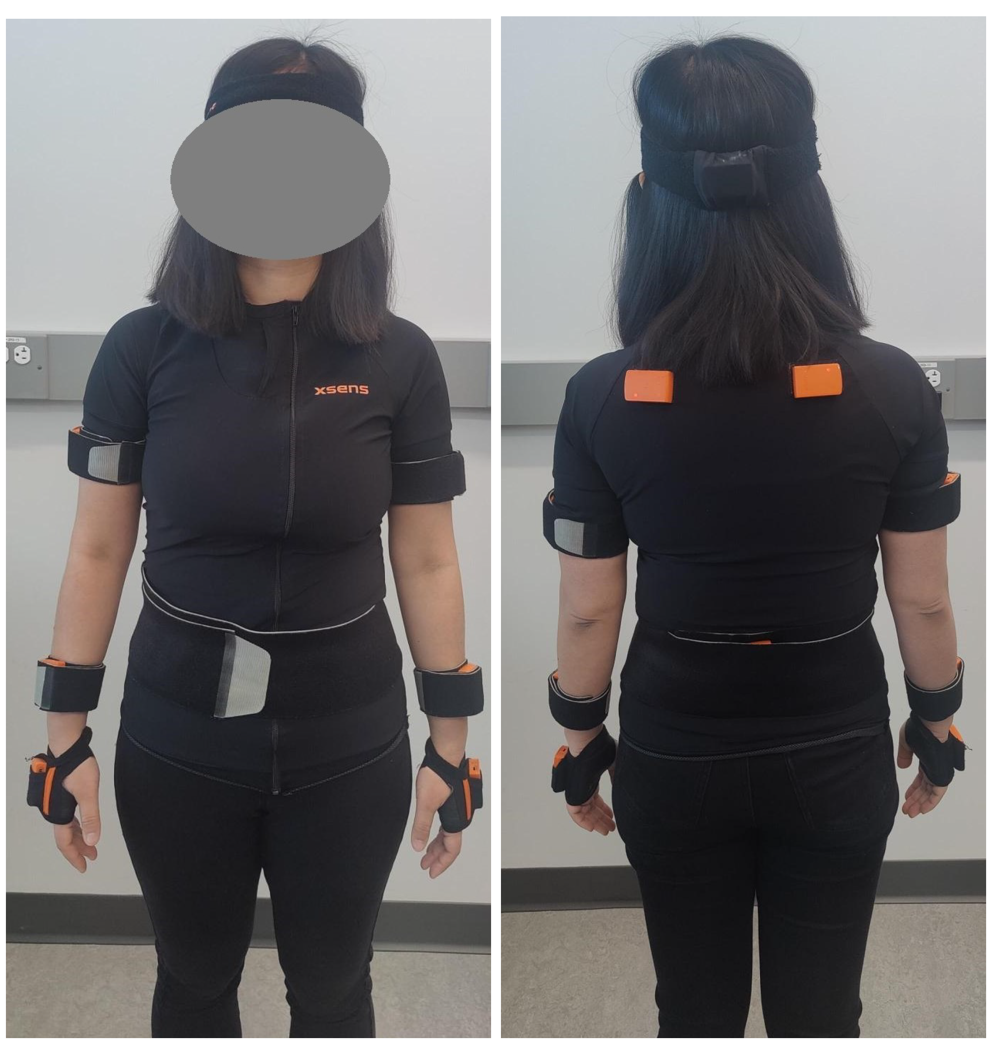
Demonstrations were collected using the Xsens Awinda motion capture suit and software (https://www.movella.com/products/xsens (accessed on 30 September 2024)), which uses Inertial Measurement Unit (IMU) data to estimate human poses [41] at 60 frames per second. The sensors are worn by the demonstrator, which is shown in Figure 2. The Cartesian position and orientations were extracted by the Xsens Awinda software relative to a coordinate frame set during the calibration of the sensors. A rotational transformation was required to convert and align the axes of the hand from the Xsens IMUs from data collection to the robot end effector. This was implemented using rotations from the Scipy version 1.13.0 Python Library [42] through Euler angle rotations.

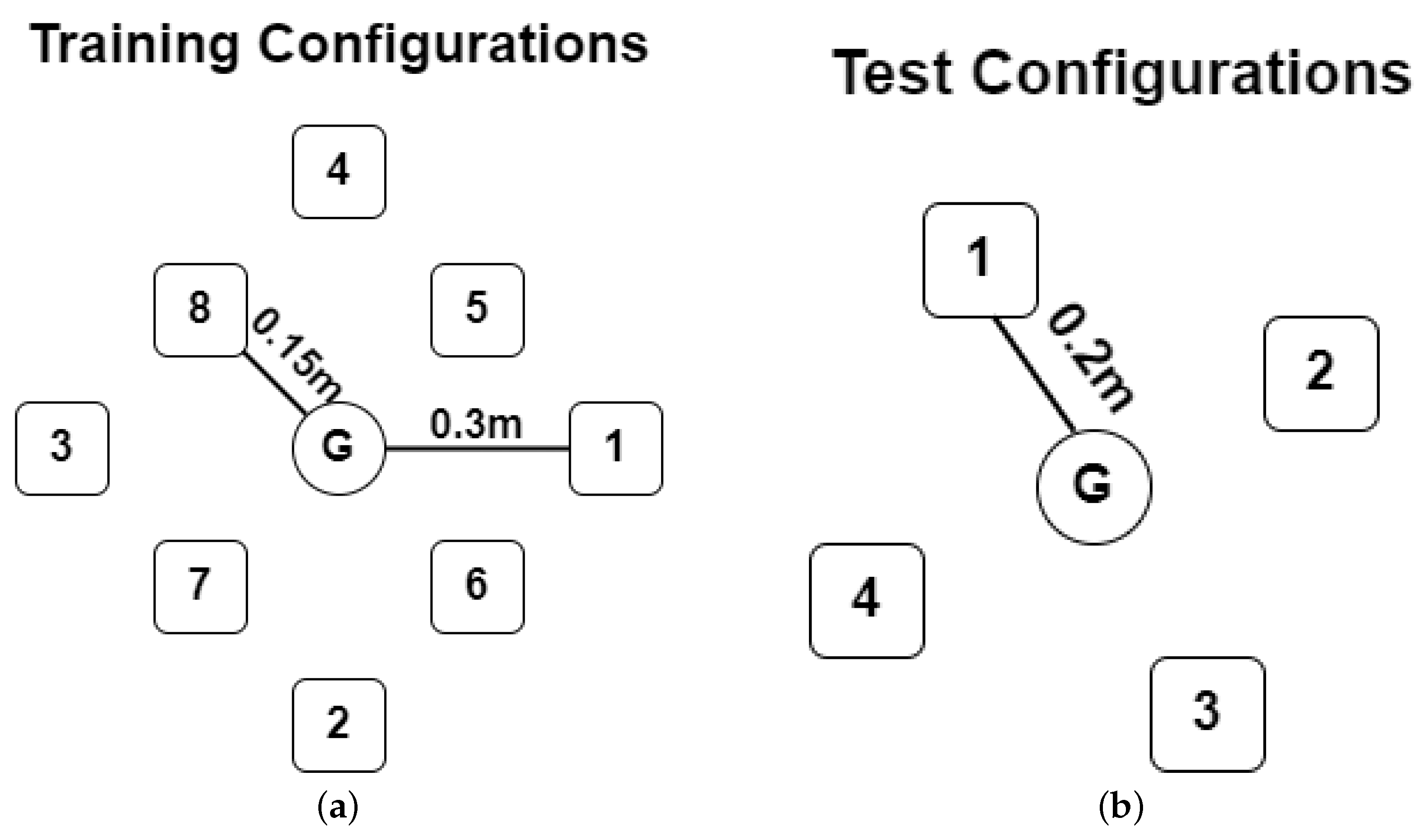
Demonstrations for the training set were collected from four demonstrators, each of which performed a pouring action in eight different configurations, shown in Figure 3a, for three different amounts of water. For each demonstrator, this took approximately half an hour, including the setup, calibration, and explanation of the demonstrations, resulting in a total demonstration collection time of 2 h. Figure 4 depicts an actual demonstration data collection session. The water levels were measured using weights, which had the following values: 799 g, 522 g, and 273 g. One participant collected demonstrations from an additional four configurations shown in Figure 3b and an additional two water levels of 397.5 g and 660.5 g to be used as a testing set. All our experiments received ethical approval from the University of Waterloo Human Research Ethics Board at the University of Waterloo, Ontario, Canada. Before the experiment, participants received proper information and gave informed consent to participate in the study.

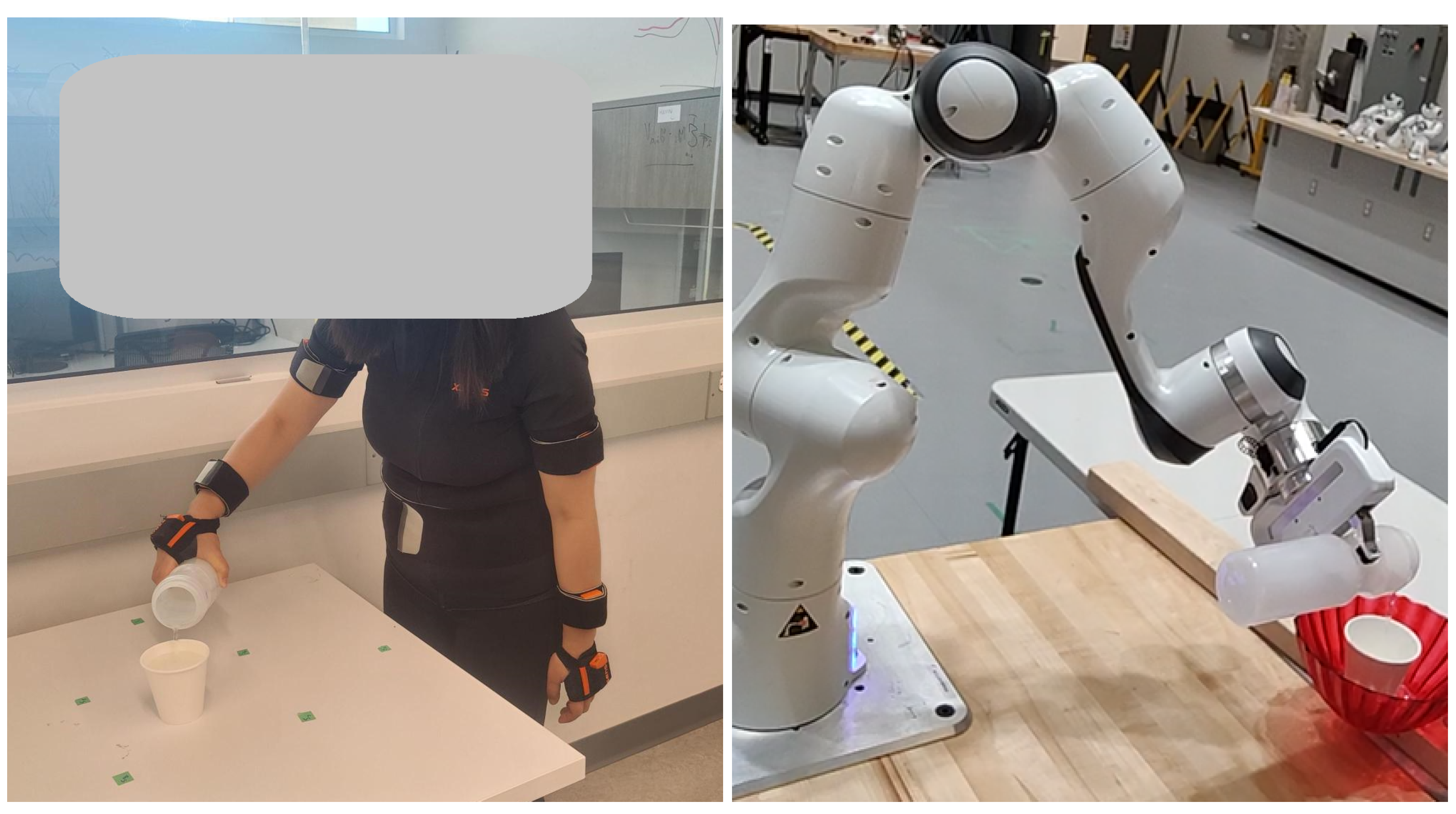
One demonstration consisted of the demonstrator starting with their hands at their sides, reaching for the pouring container, pouring into the goal container until they judged it to be full (as only the 273 g level could be entirely poured into the goal container) or the pouring container was empty, returning the pouring container to its original location, and returning their hand to their side. The demonstrators were also told to grip the container in a specific region that was suitable for a robot gripper to grasp. While it was not a specific exclusion criterion, each of the demonstrators was right-handed and used their dominant hand to pour. The position of the pouring container was varied around the goal container, as seen in Figure 3a,b, where the goal position is shown as a circle, while the pouring container positions are shown as rectangles.

The trajectories were resampled using cubic splines to ensure consistent numbers of data points. The orientation trajectories of the demonstrator’s pouring hand were used to learn a forcing function with LWR to create the labels for the orientation model, while the position trajectory of the demonstrator was used directly as the label for the position model. The implementation of a full vision system was beyond the scope of this project, as the same system would be added to frameworks using the full and segmented demonstrations and would not meaningfully impact the comparison. Additionally, the input features for the models consisted of elements that could feasibly be extracted from image feature extractors. As such, features manually extracted from the demonstrations and environment configuration were used. They included the starting position and orientation of the demonstrator’s hand, the Cartesian position of the pouring container, and the goal container, and the water level normalized to between 0 (empty) and 1 (largest water level). The inputs also included the position difference between the pouring container and the goal container, as well as between the starting hand position and the pouring container in each Cartesian axis.

The collected demonstrations were segmented into three sub-tasks to train one set of DMPs for the pouring task. The first segment included reaching for the container with water and required the end effector to navigate the environment, avoiding the goal container. The second segment began when the manipulator grasped the container and consisted of transporting the container to the goal container, pouring the water, and returning the container to its original location. This segment required the associated DMP to capture the pouring motion, including factors such as the angle at which the pouring container is tilted and the location of the end effector to successfully pour into the receiving container, while also navigating the environment to avoid collisions with the goal container. The final segment started after the pouring container had been released and required the manipulator to return to its initial position without colliding with any containers.

The segmentation points for this task were selected to best align with the input features and to best suit the DMP formulation. Each section was aligned with the available inputs to the system, with each segment beginning and ending at one of the locations specified in the input vector. The first segment, reaching for the pouring container, began at the initial position and ended at the specified position of the pouring container. The third segment, returning from the pouring container to the initial position, used the same two positions but in opposite order. The second segment started and ended at the initial position of the pouring container. Breaking the task into segments with defined starting and ending points based on information from the environment helped ensure the neural DMP had the necessary inputs required to learn the desired trajectories. These points also represented points of low velocity in the demonstrations, which helped with the segmentation process and was compatible with the standard formulation of DMPs.

The data were segmented through a combination of automated analysis and manual point selection. After applying a low-pass filter to the demonstration, the Cartesian velocity of the demonstrator’s pouring hand was used as an input for the data segmentation. The velocity components were combined to find the magnitude of the velocity and were input into the SciPy peak detection algorithm [42], which identified key points in the velocity profiles. The key points were used to define segmentation candidates, which were presented to the human supervisor. The human supervisor then used their experience and task knowledge to approve the suggested segmentation points or select new and appropriate segmentation points. Every demonstration of the same segment was normalized to be completed in a fixed time.

4.1. Dataset Formulation and Augmentation

The training datasets for the position and orientation models are described in this section. The position dataset was formulated as follows:

$${\{{\mathit{u}}_j,{\mathit{y}}_j^{demo}\}}_{j=1}^M$$

(13)

where ${\mathit{u}}_j\in {\mathbb{R}}^K$ is a vector of input features with K features, ${\mathit{y}}_j^{demo}\in {\mathbb{R}}^{T_j\times 3}$ values are the Cartesian position trajectories, and M is the number of training pairs. The input vector remains the same as the position dataset; however, the output consists of two components, as shown in Equation (14).

$${\{{\mathit{u}}_j,({\mathit{f}}_j^{demo},{\mathit{q}}_{g,j})\}}_{j=1}^M$$

(14)

where ${\mathit{f}}_j^{demo}\in {\mathbb{R}}^{T_j\times 3}$ are terms for each of the three dimensions used for the quaternion DMP formulation calculated using LWR. ${\mathit{q}}_{g,j}$ is the final orientation in the form of a quaternion and was added to the dataset so the neural DMP could learn the goal orientation as well as the weights and used during the simulation of the DMP.

To reduce the over-fitting caused by the exposure of the model to repeated identical input values, a small random deviation was added to each of the environment parameters that made up the inputs. This included the position of the goal container and pouring container, along with the initial position and orientation of the demonstrator’s pouring hand. The deviation was sampled from a normal distribution and served to ensure the model could generalize to different starting and environment parameters.

4.2. Training and Validation Sets for Cross Fold Validation

With the augmented datasets collected, the training and validation datasets for the training process described in Section 3.6 were created. For this task, the training dataset was split into four folds, with each fold removing two configurations for the validation set and the remaining six configurations were used for training. The configurations removed for each fold were selected to be far from each other to ensure the model’s training samples were still distributed across the workspace. This resulted in the following pairing of configurations to remove for each fold, with the configuration number denoted with a capital letter “C” followed by the location of the starting container given by Figure 3a.

• Fold 1: C1 and C8 used for validation;
• Fold 3: C2 and C5 used for validation;
• Fold 3: C3 and C6 used for validation;
• Fold 4: C4 and C7 used for validation.

The datasets were created from the augmented dataset, and the number of samples in the training and validation sets for each fold can be seen in

Table 1. Number of samples in each dataset before and after augmentation.

Dataset	Sample Before Augmentation	Samples After Augmentation
Full Train	96	4704
Full Test	8	392
Fold Train	72	3528
Fold Validation	24	1176

. For the remainder of the paper, “C” followed by a number indicates a training/validation configuration, and “V” followed by a number indicates a testing configuration, with the number corresponding to the configurations in Figure 3a and Figure 3b, respectively. “L” followed by a number indicates the water level described earlier in this section, with levels 1–3 indicating the levels in the training set from least to most and levels 4–5 indicating the levels in the test data set from least to most.

5. Results

This section presents the results of the models trained from the full demonstrations and from the models trained using the segmented demonstrations. First, it presents the losses from the complete datasets, followed by an analysis of the individual trajectories. It also demonstrates the implementation of the pouring task on the physical robot manipulator.

5.1. Model Losses

The average losses from the position models are presented in

Table 2. Training, validation, and testing losses for each of the position models and the average loss across all segments weighted by segment lengths. Cross-validation losses are averaged across each fold shown in Table A1 in Appendix A.1.

	Position
	Cross Validation		Full
Model	Avg. Train	Avg. Val.	Train	Test
Full	0.00142	0.00239	0.00123	0.00289
Segment 1	0.00112	0.00127	0.00104	0.00139
Segment 2	0.000903	0.00155	0.000866	0.000904
Segment 3	0.00133	0.00153	0.00129	0.00151
Avg. Segments	0.00106	0.00148	0.00102	0.00118

, and the average losses from the orientation models are presented in

Table 3. Training, validation, and testing losses for each of the orientation models of the average loss across all segments weighted by segment lengths. Cross-validation losses are averaged across each fold shown in Table A2 in Appendix A.1.

	Orientation
	Cross Validation		Full
Model	Avg. Train	Avg. Val.	Train	Test
Full	0.415	0.459	0.404	0.463
Segment 1	0.399	0.455	0.367	0.447
Segment 2	0.441	0.536	0.329	0.456
Segment 3	0.322	0.406	0.300	0.335
Avg. Segments	0.401	0.484	0.332	0.424

. Both of these tables show the average losses for each of the models, including the model learned from the full demonstrations and the models learned from each of the segments. The average over the entire trajectory of the segmented models, weighted by the length of each segment, is also presented as a method of evaluating the loss over the full trajectory for the segmented models.

The loss for the position models was calculated using the Euclidean distance between the predicted and demonstrated trajectories, while the logarithmic mapping shown in Equation (10) was used to measure the distance between the demonstrated and predicted orientation quaternion trajectories. The losses were averaged over each trajectory and then over the full dataset.

The average losses for each of the models were larger for the test set than for the training set, including during the cross-validation. Additionally, by comparing the weighted average loss of the segmented models to the full model, we can see that the segmented version has a lower average loss, indicating a high accuracy.

5.2. Model Trained on Full Demonstrations

The position and orientation models trained on the full demonstrations used the parameters shown in

Table 4. Model parameters for the position and orientation neural DMPs trained on the full demonstrations.

Parameter	Position	Orientation
number of layers	3	3
layer sizes	300, 200, 300	700, 400, 300
$\beta$	25	25
epochs	40	7
number of basis functions	50	50

. Each neural network was composed of three dense layers, and the number of epochs was 40 epochs for the position model and 7 epochs for the orientation model. Rectified linear unit (ReLU) activation functions were used following each layer in each of the networks.

5.2.1. Training Set Performance

The three configurations of the pouring and receiving container selected from the training set for visualization each had a different water level and were selected to analyze the recall of the models. The Cartesian components of the position trajectories from the demonstrations and the corresponding position trajectories generated from the neural DMP for the selected samples are shown in Figure 5. The corresponding quaternion orientation trajectories from the demonstrations and the predicted orientation trajectories from the neural DMP are shown in Figure 6. In both cases, the demonstrated trajectory components are shown by a solid black line, while the predicted trajectory components are shown with a dashed red line.

From the selected trajectories, we can see the neural DMPs that used the full demonstrations while training are able to recall the shape of trajectories from the training set. They are able to reproduce the shape of the demonstrations. However, there appears to be more error near the end of the demonstrations in both the position and orientation plots in Figure 5 and Figure 6.

5.2.2. Testing Set Performance

The two configurations of the pouring and receiving containers selected from the testing dataset had different water levels and were selected to assess the generalization capabilities of the models. The Cartesian components of the position trajectories from the demonstrations and the corresponding position trajectories generated from the neural DMP for the selected samples are shown in Figure 7. The corresponding quaternion orientation trajectories from the demonstrations and the predicted orientation trajectories from the neural DMP are shown in Figure 8. As with the training set, the demonstrated trajectory components are shown by a solid black line, while the predicted trajectory components are shown with a dashed red line for both figures.

Figure 7 and Figure 8 show that while the models trained from the full demonstrations are able to maintain the general shape of the demonstrations of an expert, there is increased error compared to the demonstrations from the training set. This is expected to a certain extent as a byproduct of neural networks, which are not able to generalize perfectly, and is also found in other works on neural DMPs [43]. However, this is also likely a result of the neural networks learning from multiple demonstrators. By incorporating demonstrations from multiple humans, the neural network should learn the common elements between the demonstrators. As such, it may cause the models to miss some elements from single demonstrators when generalizing, as it has learned the commonalities across all the demonstrators, which could account for some of the errors. Despite the increased error, examining these two plots shows the key movements stay aligned in time with the demonstrations. This shows that while the movements may not be exactly the same as the demonstrator, they maintain similar elements at similar times and maintain the structure of the underlying task. As such, this shows that the models have learned key features of the task, and the errors may be explained by learning the commonalities between demonstrators instead of replicating a single demonstrator.

5.3. Model Trained on Segmented Demonstrations

The same configurations and water levels were selected for the segmented models as were selected for the models trained on the full demonstrations, allowing for a comparison between the two methods. As such, three samples and configurations were selected from the training set, and two configurations were selected from the testing set. The parameters for each position segment model are presented in

Table 5. Model parameters for the position of neural DMPs trained on the segmented demonstrations for each segment.

	Position Models
Parameter	Seg. 1	Seg. 2	Seg. 3
number of layers	1	1	1
layer sizes	230	340	140
$\beta$	20	20	20
epochs	14	14	12
number of basis functions	20	40	15

, and the parameters for each orientation segment model are presented in

Table 6. Model parameters for the orientation of neural DMPs trained on the segmented demonstrations for each segment.

	Orientation Models
Parameter	Seg. 1	Seg. 2	Seg. 3
number of layers	2	3	2
layer sizes	110, 110	200, 230, 200	170, 230
$\beta$	25	25	25
epochs	11	10	7
number of basis functions	10	30	10

. The models were composed of fully connected layers. It can be seen that for both the position and orientation models, the first and third segments tend to have simpler models than the second in terms of the number of layers, the number of nodes per layer, and the number of basis functions. This is because they represent the more basic motions of reaching for the container and returning to the original manipulator position, while segment 1 represents a more complex motion that requires the actual pouring of the liquid. ReLU activation functions were used following each layer in each of the networks.

5.3.1. Training Set Performance

The trajectories and demonstrations from the same three configurations with the same water levels that were shown for the models generated from the full demonstrations are displayed for the models trained using the segmented demonstrations. The Cartesian components of the position trajectories from the demonstrations and the corresponding position trajectories generated from the neural DMP for the selected samples are shown in Figure 9. The corresponding quaternion orientation trajectories from the demonstrations and the predicted orientation trajectories from the neural DMP are shown in Figure 10. In both cases, the demonstrated trajectory components are shown by a solid black line, the predicted trajectory components are shown with a dashed red line, and the locations where the demonstration segmentation occurred are shown using a vertical blue dashed line.

Figure 9 and Figure 10 show that the neural DMPs trained using the segmented models are, for the most part, able to accurately reproduce previously seen trajectories. When comparing the third orientation trajectory (bottom left) from the segmented demonstration method in Figure 10 to the corresponding trajectory from the full demonstration method in Figure 5, it appears to have a larger error, particularly near the middle of the trajectory. This seems to contradict the average losses presented in Section 5.1, which are typically lower for the segmented models. However, this serves to demonstrate that while average losses may be lower for the segmented models, there may be individual trajectories that are better represented by the models trained using full demonstrations. Also, unlike the models that used the full demonstrations, the segmented models appear to have more consistent errors throughout the trajectory as opposed to increased errors near the end of the demonstration.

5.3.2. Testing Set Performance

Once again, the same configurations and water levels that were used to demonstrate the test performance for the neural DMPs that were trained using the full demonstrations are shown to demonstrate the generalization capabilities of the segmented models. The Cartesian components of the position trajectories from the demonstrations, and the corresponding position trajectories generated from the neural DMP for the selected samples are shown in Figure 11. The corresponding quaternion orientation trajectories from the demonstrations and the predicted orientation trajectories from the neural DMP are shown in Figure 12. As with the training set, the demonstrated trajectory components are shown by a solid black line, the predicted trajectory components are shown with a dashed red line, and the segmentation points are shown with dashed blue lines for both figures.

As shown in Figure 11 and Figure 12, the position and orientation generated by the segmented neural DMPs are similar to those of the demonstrator. However, just as with the models trained on the full demonstrations, there is an increased error, which is expected as a result of neural networks not generalizing perfectly. Similarly, this is also likely due to the models having learned from different demonstrators, thus incorporating elements from the training trajectories from various demonstrations. This means that it may not perfectly align with a single demonstrator when generalizing, which could account for some of the error. Despite the increased error, examining these two plots shows that the key movements stay aligned in time with the demonstrations. This shows that while the movements may not be exactly the same as the demonstrator, they maintain similar elements at similar times. As with the models learned from full demonstrations, this shows that while the movements may not be exactly the same as the demonstrator, they maintain similar elements at similar times and maintain the structure of the underlying task. As such, this shows that the models have learned key features of the task, and the errors may be due to the learning base explained by learning the commonalities between demonstrators instead of replicating a single demonstrator.

5.4. Performance of the Robotic System

Both the models trained on the full demonstrations and those trained on the segmented demonstrations were implemented on the Franka Emika Panda 7DoF robot manipulator. A sequence of images showing the task completion for both sets of models can be seen in Figure 13. This corresponds to the first configuration and water level selected in the previous sections for the plotted trajectories. This was tested for multiple configurations and water levels and was found to be capable of completing the task. Additional examples can be seen in the video attachment.

6. Discussion

When comparing the models generated from the full demonstrations to those that utilized the segmented demonstrations, several factors are considered. These include the accuracy of the models on cases seen and not seen during training, the amount of expert human input that was required, and the potential for task flexibility within the framework. These factors, and how they relate to the desired application, should also be taken into account when selecting whether to use full or segmented demonstrations. The desired accuracy, availability of demonstrations, expected timeline, and task complexity should be balanced with the trade-offs of the different methods to select a suitable strategy. For example, segmented demonstrations may be appropriate for a maintenance task such as replacing a component in machinery, which is composed of distinct sub-tasks. Learning from full demonstrations on the other hand may be more well suited to manipulating human joints during rehabilitation, where there are fewer distinct sub-tasks, and would require large amounts of time from physicians to annotate demonstrations. However, this paper is not meant to be a guide for selecting a method, as the variability of applications and factors is large. Instead, this paper aims to present some of the trade-offs between the two methods, which the reader can use in the context of their application.

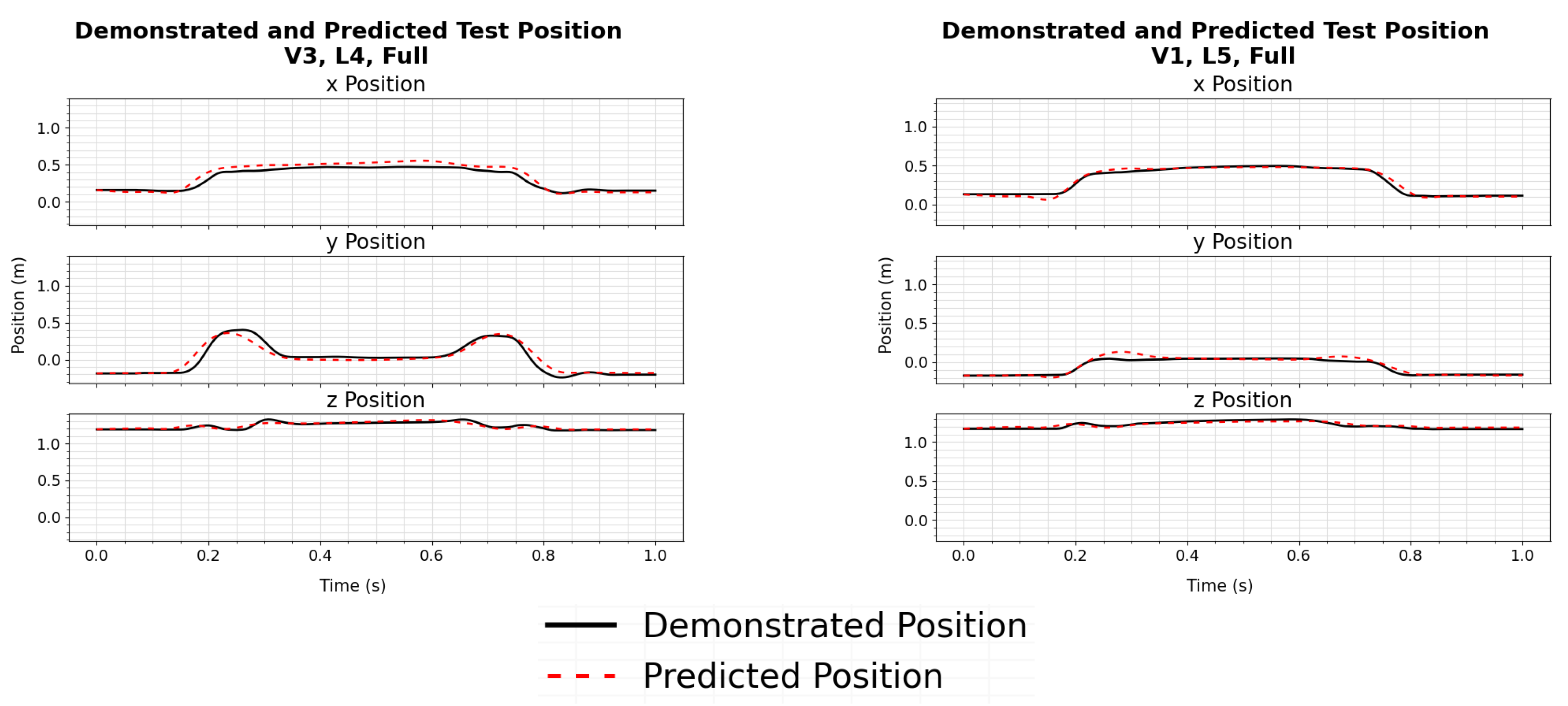
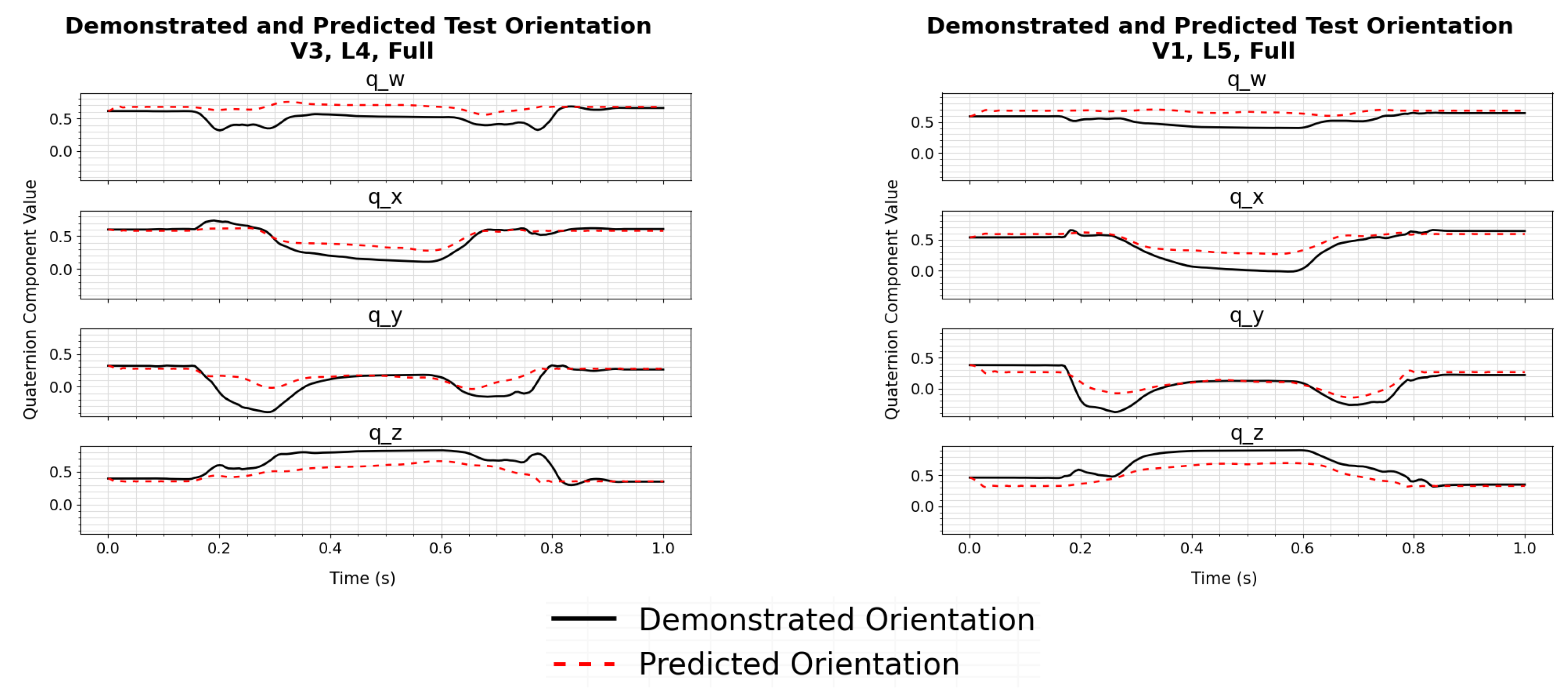
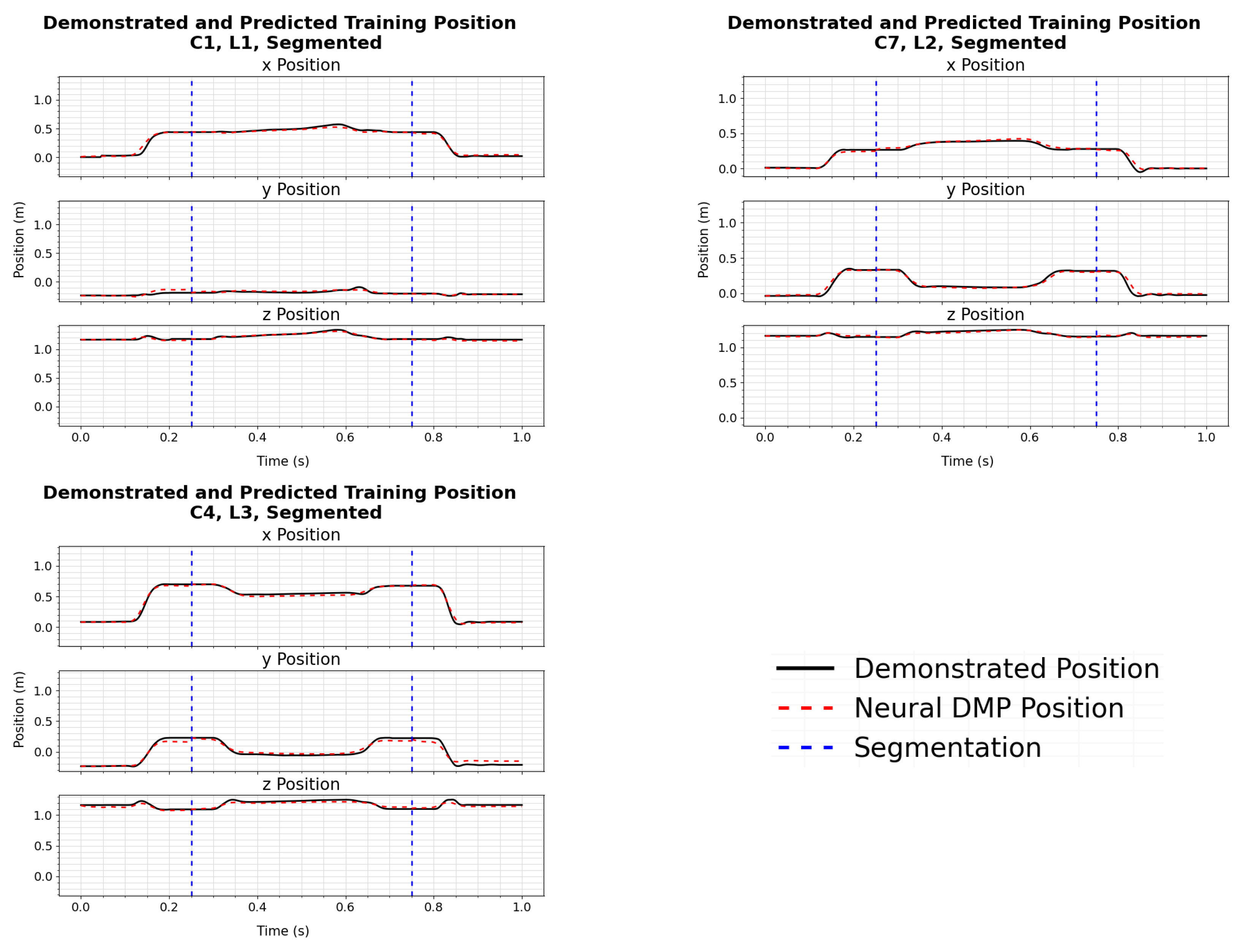
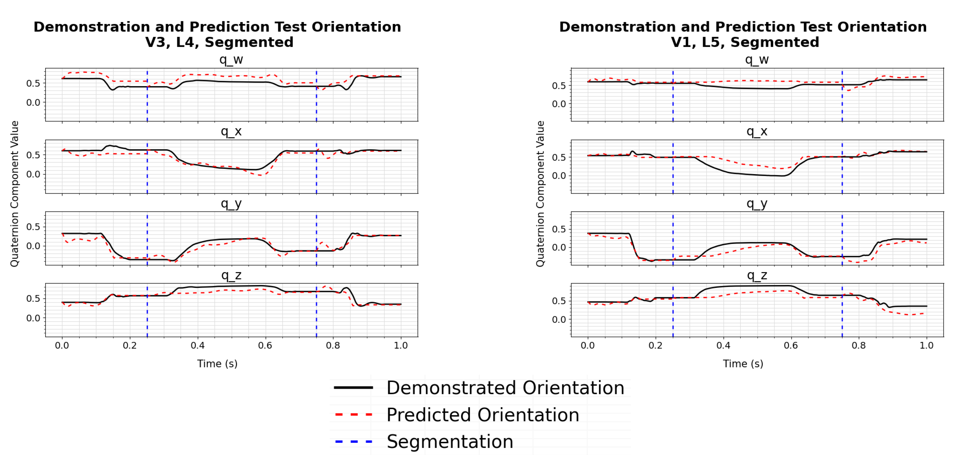
The results show that the models trained from the segmented demonstrations are more accurate in determining the correct trajectories for configurations seen during training, and new configurations. This can be seen over the full set of trajectories by comparing the losses in Table 2 and Table 3. This can also be seen by comparing individual sample trajectories generated from models trained using full demonstrations in Figure 5, Figure 6, Figure 7 and Figure 8 to the corresponding sample trajectories from models trained using segmented trajectories in Figure 9, Figure 10, Figure 11 and Figure 12. 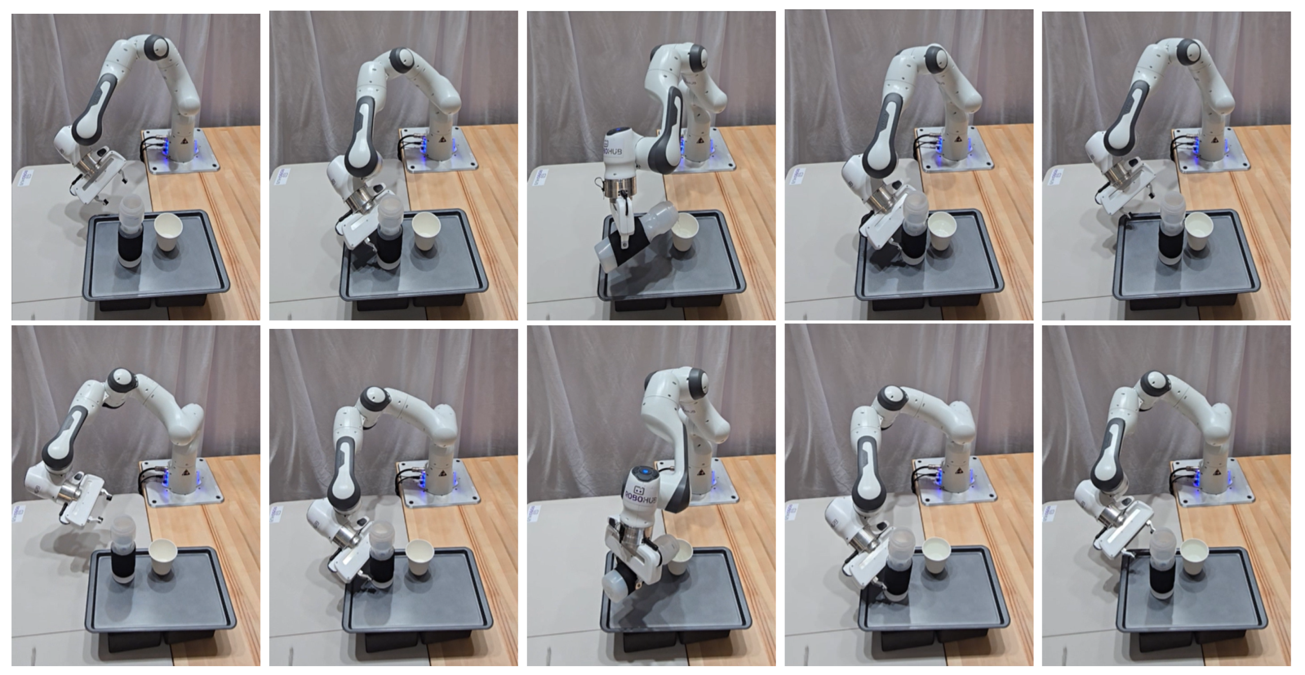In particular, the trajectories from the models trained using full demonstrations show increased error in later sections of the trajectories, which is similar to the position and orientation trajectories presented in [14,17]. While both the full and segmented trajectories were successfully implemented on the physical robotic system, the difference in accuracy could have a larger impact for more precise tasks.

The models that learned from segmented demonstrations required additional time and effort from the expert. The main source of added time was the segmentation and annotation of the demonstrations, as discussed in Section 4, and required an additional 2 weeks to design the semi-automated segmentation and to supervise the segmentation. While this was feasible for the relatively simple task presented in this paper, it would require additional time for more complex tasks. This could be further extended in cases where more demonstrations are required, or where the experimentation of the segmentation points need to be experimented with to successfully learn a task.

The segmented models could achieve a higher task flexibility than the full models, largely due to their potential to be combined into new sequences or used for new tasks. For example, the reaching segment used in the pouring task could be reused for other tasks that require this motion, such as sorting tasks or assembly tasks. A relatively simple high-level planner was used in this paper, but this could be extended further to incorporate additional functionality, such as confirming each sub-task is complete before moving to the next [25]. In comparison, the models trained on full demonstrations would require new demonstrations and full re-training to be applied to different applications and would require structural changes to implement higher-level frameworks.

7. Conclusions

This paper presents a framework that uses neural DMPs for skill transfer between humans and a robot manipulator. The neural DMPs were trained to complete a pouring task using full demonstrations and demonstrations segmented into individual sub-tasks. The neural DMPs required a small number of demonstrations, requiring only 24 human examples, to learn and generalize for a pouring task and were able to generalize to new configurations of the task not seen during training. The neural DMP formulation and robot control strategy were discussed, followed by a description and analysis of the demonstration, collection, training, and testing processes, as well as an implementation of a Franka Emika Panda 7-DoF manipulator. This allowed for a comparison of the accuracy of each method while also allowing for some analysis of the input requirements from a human expert and the task flexibility of each method.

Several trade-offs between the models trained on full demonstrations and the models trained on segmented demonstrations were discussed. It was found that the model trained using the segmented demonstrations had a higher accuracy on the training and testing datasets, indicating that shorter motion primitives could increase the accuracy. Additionally, the models trained on segmented demonstrations are anticipated to have higher task flexibility, requiring fewer changes to the framework and minimal retraining to be applied to new tasks. However, the segmentation and annotation of the demonstrations required for this method significantly increased the amount of time required by the expert as they are required to both perform and annotate the demonstrations.

While this paper provides an in-depth comparison between neural DMP models that learn from a full demonstration to models that learn from sub-tasks, future work could expand on this comparison. This could include analyzing the differences in performance for tasks with different lengths and complexities or finding the ideal locations of how to subdivide different tasks. Further work could also be performed to assess the suitability of sub-tasks to transfer to new skills.

References

1. Arents, J.; Greitans, M. Smart industrial robot control trends, challenges and opportunities within manufacturing. Appl. Sci. 2022, 12, 937. [Google Scholar] [CrossRef]
2. González, C.; Solanes, J.E.; Muñoz, A.; Gracia, L.; Girbés-Juan, V.; Tornero, J. Advanced teleoperation and control system for industrial robots based on augmented virtuality and haptic feedback. J. Manuf. Syst. 2021, 59, 283–298. [Google Scholar] [CrossRef]
3. Ziheng, W.; Reed, I.; Fey, A.M. Toward Intuitive Teleoperation in Surgery: Human-centric Evaluation of Teleoperation Algorithms for Robotic Needle Steering. In Proceedings of the 2018 IEEE International Conference on Robotics and Automation (ICRA), Brisbane, Australia, 21–25 May 2018. [Google Scholar]
4. Riek, L.D. Chapter 8-Robotics Technology in Mental Health Care. In Artificial Intelligence in Behavioral and Mental Health Care; Luxton, D.D., Ed.; Academic Press: San Diego, CA, USA, 2016; pp. 185–203. [Google Scholar] [CrossRef]
5. Yuan, F.; Klavon, E.; Liu, Z.; Lopez, R.P.; Zhao, X. A systematic review of robotic rehabilitation for cognitive training. Front. Robot. AI 2021, 8, 605715. [Google Scholar] [CrossRef] [PubMed]
6. Pistone, A.; Ludovico, D.; De Mari Casareto Dal Verme, L.; Leggieri, S.; Canali, C.; Caldwell, D.G. Modelling and control of manipulators for inspection and maintenance in challenging environments: A literature review. Annu. Rev. Control 2024, 57, 100949. [Google Scholar] [CrossRef]
7. Paul, G.; Webb, S.; Liu, D.; Dissanayake, G. Autonomous robot manipulator-based exploration and mapping system for bridge maintenance. Robot. Auton. Syst. 2011, 59, 543–554. [Google Scholar] [CrossRef]
8. Fang, B.; Jia, S.; Guo, D.; Xu, M.; Wen, S.; Sun, F. Survey of imitation learning for robotic manipulation. Int. J. Intell. Robot. Appl. 2019, 3, 362–369. [Google Scholar] [CrossRef]
9. Schaal, S.; Mohajerian, P.; Ijspeert, A. Dynamics systems vs. optimal control—A unifying view. In Computational Neuroscience: Theoretical Insights into Brain Function; Progress in Brain Research; Cisek, P., Drew, T., Kalaska, J.F., Eds.; Elsevier: Amsterdam, The Netherlands, 2007; Volume 165, pp. 425–445. [Google Scholar] [CrossRef]
10. Rožanec, J.M.; Nemec, B. Neural Dynamic Movement Primitives—A survey. arXiv 2022, arXiv:2208.01903. [Google Scholar]
11. Bahl, S.; Mukadam, M.; Gupta, A.; Pathak, D. Neural Dynamic Policies for End-to-End Sensorimotor Learning. In Proceedings of the Advances in Neural Information Processing Systems; Larochelle, H., Ranzato, M., Hadsell, R., Balcan, M., Lin, H., Eds.; Curran Associates, Inc.: San Francisco, CA, USA, 2020; Volume 33, pp. 5058–5069. [Google Scholar]
12. Misimi, E.; Olofsson, A.; Eilertsen, A.; Øye, E.R.; Mathiassen, J.R. Robotic Handling of Compliant Food Objects by Robust Learning from Demonstration. In Proceedings of the 2018 IEEE/RSJ International Conference on Intelligent Robots and Systems (IROS), Madrid, Spain, 1–5 October 2018; pp. 6972–6979. [Google Scholar] [CrossRef]
13. Schaal, S. Dynamic Movement Primitives—A Framework for Motor Control in Humans and Humanoid Robotics. In Adaptive Motion of Animals and Machines; Springer: Tokyo, Japan, 2006; pp. 261–280. [Google Scholar] [CrossRef]
14. Saveriano, M.; Abu-Dakka, F.J.; Kramberger, A.; Peternel, L. Dynamic movement primitives in robotics: A tutorial survey. Int. J. Robot. Res. 2023, 42, 1133–1184. [Google Scholar] [CrossRef]
15. Abu-Dakka, F.J.; Nemec, B.; Jørgensen, J.A.; Savarimuthu, T.R.; Krüger, N.; Ude, A. Adaptation of manipulation skills in physical contact with the environment to reference force profiles. Auton. Robot. 2015, 39, 199–217. [Google Scholar] [CrossRef]
16. Ude, A.; Nemec, B.; Petrić, T.; Morimoto, J. Orientation in Cartesian space dynamic movement primitives. In Proceedings of the 2014 IEEE International Conference on Robotics and Automation (ICRA), Hong Kong, China, 31 May–7 June 2014; pp. 2997–3004. [Google Scholar] [CrossRef]
17. Saveriano, M.; Franzel, F.; Lee, D. Merging Position and orientation Motion Primitives. In Proceedings of the 2019 International Conference on Robotics and Automation (ICRA), Montreal, QC, Canada, 20–24 May 2019; pp. 7041–7047. [Google Scholar] [CrossRef]
18. Si, W.; Wang, N.; Yang, C. Composite dynamic movement primitives based on neural networks for human–Robot skill transfer. Neural Comput. Appl. 2021, 35, 23283–23293. [Google Scholar] [CrossRef]
19. Joshi, R.P.; Koganti, N.; Shibata, T. Robotic cloth manipulation for clothing assistance task using Dynamic Movement Primitives. In Proceedings of the 2017 3rd International Conference on Advances in Robotics. Association for Computing Machinery, New Delhi, India, 28 June–2 July 2017. [Google Scholar] [CrossRef]
20. Ravichandar, H.; Polydoros, A.S.; Chernova, S.; Billard, A. Recent advances in robot learning from demonstration. Annu. Rev. Control. Robot. Auton. Syst. 2020, 3, 297–330. [Google Scholar] [CrossRef]
21. Zhou, Y.; Gao, J.; Asfour, T. Learning Via-Point Movement Primitives with Inter- and Extrapolation Capabilities. In Proceedings of the 2019 IEEE/RSJ International Conference on Intelligent Robots and Systems (IROS), Macau, China, 3–8 November 2019; pp. 4301–4308. [Google Scholar] [CrossRef]
22. Sidiropoulos, A.; Doulgeri, Z. Dynamic Via-points and Improved Spatial Generalization for Online Trajectory Generation with Dynamic Movement Primitives. J. Intell. Robot. Syst. 2024, 110, 24. [Google Scholar] [CrossRef]
23. Pastor, P.; Hoffmann, H.; Asfour, T.; Schaal, S. Learning and generalization of motor skills by learning from demonstration. In Proceedings of the 2009 IEEE International Conference on Robotics and Automation, Kobe, Japan, 12–17 May 2009; IEEE: Piscataway Township, NJ, USA, 2009; pp. 763–768. [Google Scholar]
24. Caccavale, R.; Saveriano, M.; Finzi, A.; Lee, D. Kinesthetic teaching and attentional supervision of structured tasks in human–robot interaction. Auton. Robot. 2019, 43, 1291–1307. [Google Scholar] [CrossRef]
25. Luo, J.; Xu, C.; Geng, X.; Feng, G.; Fang, K.; Tan, L.; Schaal, S.; Levine, S. Multistage Cable Routing Through Hierarchical Imitation Learning. IEEE Trans. Robot. 2024, 40, 1476–1491. [Google Scholar] [CrossRef]
26. Xie, F.; Chowdhury, A.; Kaluza, M.C.D.P.; Zhao, L.; Wong, L.; Yu, R. Deep Imitation Learning for Bimanual Robotic Manipulation. In Proceedings of the Advances in Neural Information Processing Systems; Larochelle, H., Ranzato, M., Hadsell, R., Balcan, M.F., Lin, H., Eds.; Curran Associates, Inc.: San Francisco, CA, USA, 2020; Volume 33, pp. 2327–2337. [Google Scholar]
27. Matsubara, T.; Hyon, S.H.; Morimoto, J. Learning Stylistic Dynamic Movement Primitives from multiple demonstrations. In Proceedings of the 2010 IEEE/RSJ International Conference on Intelligent Robots and Systems, Taipei, Taiwan, 18–22 October 2010; pp. 1277–1283. [Google Scholar] [CrossRef]
28. Krug, R.; Dimitrov, D. Model Predictive Motion Control based on Generalized Dynamical Movement Primitives. J. Intell. Robot. Syst. 2015, 77, 17–35. [Google Scholar] [CrossRef]
29. Krug, R.; Dimitrovz, D. Representing movement primitives as implicit dynamical systems learned from multiple demonstrations. In Proceedings of the 2013 16th International Conference on Advanced Robotics (ICAR), Montevideo, Uruguay, 25–29 November 2013; pp. 1–8. [Google Scholar] [CrossRef]
30. Chen, C.; Yang, C.; Zeng, C.; Wang, N.; Li, Z. Robot learning from multiple demonstrations with dynamic movement primitive. In Proceedings of the 2017 2nd International Conference on Advanced Robotics and Mechatronics (ICARM), Tai’an, China, 27–31 August 2017; pp. 523–528. [Google Scholar] [CrossRef]
31. Dong, S.; Yang, Z.; Zhang, W.; Zou, K. Dynamic movement primitives based on positive and negative demonstrations. Int. J. Adv. Robot. Syst. 2023, 20, 17298806231152997. [Google Scholar] [CrossRef]
32. Hu, Y.; Cui, M.; Duan, J.; Liu, W.; Huang, D.; Knoll, A.; Chen, G. Model predictive optimization for imitation learning from demonstrations. Robot. Auton. Syst. 2023, 163, 104381. [Google Scholar] [CrossRef]
33. Ginesi, M.; Sansonetto, N.; Fiorini, P. Overcoming some drawbacks of Dynamic Movement Primitives. Robot. Auton. Syst. 2021, 144, 103844. [Google Scholar] [CrossRef]
34. Racinskis, P.; Arents, J.; Greitans, M. A motion capture and imitation learning based approach to Robot Control. Appl. Sci. 2022, 12, 7186. [Google Scholar] [CrossRef]
35. Pervez, A.; Mao, Y.; Lee, D. Learning deep movement primitives using convolutional neural networks. In Proceedings of the 2017 IEEE-RAS 17th International Conference on Humanoid Robotics (Humanoids), Birmingham, UK, 15–17 November 2017; pp. 191–197. [Google Scholar] [CrossRef]
36. Pahič, R.; Ridge, B.; Gams, A.; Morimoto, J.; Ude, A. Training of deep neural networks for the generation of dynamic movement primitives. Neural Netw. 2020, 127, 121–131. [Google Scholar] [CrossRef]
37. Chen, N.; Bayer, J.; Urban, S.; van der Smagt, P. Efficient movement representation by embedding Dynamic Movement Primitives in deep autoencoders. In Proceedings of the 2015 IEEE-RAS 15th International Conference on Humanoid Robots (Humanoids), Seoul, Republic of Korea, 3–5 November 2015; pp. 434–440. [Google Scholar] [CrossRef]
38. Atkeson, C.G.; Moore, A.W.; Schaal, S. Locally Weighted Learning. In Lazy Learning; Springer: Dordrecht, The Netherlands, 1997; pp. 11–73. [Google Scholar] [CrossRef]
39. Felis, M.L. RBDL: An efficient rigid-body dynamics library using recursive algorithms. Auton. Robot. 2016, 41, 495–511. [Google Scholar] [CrossRef]
40. Liaw, R.; Liang, E.; Nishihara, R.; Moritz, P.; Gonzalez, J.E.; Stoica, I. Tune: A Research Platform for Distributed Model Selection and Training. arXiv 2018, arXiv:1807.05118. [Google Scholar]
41. Schepers, M.; Giuberti, M.; Bellusci, G. Xsens MVN: Consistent tracking of human motion using inertial sensing. Xsens Technol 2018, 1, 1–8. [Google Scholar]
42. Virtanen, P.; Gommers, R.; Oliphant, T.E.; Haberland, M.; Reddy, T.; Cournapeau, D.; Burovski, E.; Peterson, P.; Weckesser, W.; Bright, J.; et al. SciPy 1.0: Fundamental Algorithms for Scientific Computing in Python. Nat. Methods 2020, 17, 261–272. [Google Scholar] [CrossRef]
43. Zhang, Y.; Li, M.; Yang, C. Robot learning system based on dynamic movement primitives and neural network. Neurocomputing 2021, 451, 205–214. [Google Scholar] [CrossRef]
Figure 1. Control structure overview, showing the transformation of the input features through the position and orientation neural networks to predict the weight and goal parameters of their respective DMPs, which then generate trajectories. Inverse kinematics generate a joint position trajectory from the Cartesian trajectory, which the robot follows using a joint impedance controller.
Machines 12 00872 g001
Figure 2. The front (left) and back (right) of how the Xsens Awinda IMU motion capture sensors are worn by the demonstrator.
Machines 12 00872 g002
Figure 3. Configurations with pouring container locations as rectangles and the goal container as a circle. (a) Configurations used to collect demonstrations for training. (b) Configurations used to collect demonstrations for testing.
Machines 12 00872 g003
Figure 4. A demonstrator performing a pouring task (left) and a robot performing the learned pouring task (right).
Machines 12 00872 g004
Figure 5. Trajectory components of the demonstrated position and the position predicted by the neural DMP for the model trained using the full demonstrations for samples from the training dataset.
Machines 12 00872 g005
Figure 6. Trajectory components of the demonstrated orientation and the orientation predicted by the neural DMP for the model trained using the full demonstrations for samples from the training dataset.
Machines 12 00872 g006
Figure 7. Trajectory components of the demonstrated position and the position predicted by the neural DMP for the model trained using the full demonstrations for samples from the test data set.
Machines 12 00872 g007
Figure 8. Trajectory components of the demonstrated orientation and the orientation predicted by the neural DMP for the model trained using the full demonstrations for samples from the test data set.
Machines 12 00872 g008
Figure 9. Trajectory components of the demonstrated position and the position predicted by the neural DMP for the model trained using the segmented demonstrations for samples from the training dataset.
Machines 12 00872 g009
Figure 10. Trajectory components of the demonstrated orientation and the orientation predicted by the neural DMP for the model trained using the segmented demonstrations for samples from the training dataset.
Machines 12 00872 g010
Figure 11. Trajectory components of the demonstrated position and the position predicted by the neural DMP for the model trained using the segmented demonstrations for samples from the test dataset.
Machines 12 00872 g011
Figure 12. Trajectory components of the demonstrated orientation and the orientation predicted by the neural DMP for the model trained using the segmented demonstrations for samples from the test dataset.
Machines 12 00872 g012
Figure 13. Image sequence showing the first trajectory and water level (C1 L1) being performed by the robot using the neural DMPs trained on the full demonstrations (top) and using the neural DMPs trained using the segmented demonstrations (bottom). A video of the results can be seen in Supplementary Video S1.
Machines 12 00872 g013