Optimizing Project Time and Cost Prediction Using a Hybrid XGBoost and Simulated Annealing Algorithm

Abstract

Machine learning technologies have recently emerged as transformative tools for enhancing project management accuracy and efficiency. This study introduces a data-driven model that leverages the hybrid eXtreme Gradient Boosting-Simulated Annealing (XGBoost-SA) algorithm to predict the time and cost of construction projects. By accounting for the complexity of activity networks and uncertainties within project environments, the model aims to address key challenges in project forecasting. Unlike traditional methods such as Earned Value Management (EVM) and Earned Schedule Method (ESM), which rely on static metrics, the XGBoost-SA model adapts dynamically to project data, achieving 92% prediction accuracy. This advanced model offers a more precise forecasting approach by incorporating and optimizing features from historical data. Results reveal that XGBoost-SA reduces cost prediction error by nearly 50% and time prediction error by approximately 80% compared to EVM and ESM, underscoring its effectiveness in complex scenarios. Furthermore, the model’s ability to manage limited and evolving data offers a practical solution for real-time adjustments in project planning. With these capabilities, XGBoost-SA provides project managers with a powerful tool for informed decision-making, efficient resource allocation, and proactive risk management, making it highly applicable to complex construction projects where precision and adaptability are essential. The main limitation of the developed model in this study is the reliance on data from similar projects, which necessitates additional data for application to other industries.

1. Introduction

The transition to Industry 4.0 has revolutionized industries and complex projects by integrating advanced technologies, emphasizing efficiency, resource utilization, sustainability, and resilience. As noted in ‘Toward Sustainability and Resilience with Industry 4.0 and Industry 5.0 [1], these advancements set the stage for innovative approaches to project management, where hybrid machine learning techniques can significantly enhance the accuracy of project time and cost predictions, ultimately driving successful outcomes in an increasingly complex environment. The construction industry has significantly evolved due to technological advancements and innovative developments [2]. Companies that fail to leverage these capabilities may face decreased profitability and decline [3]. Proper planning is one of the most critical challenges in construction projects [4]. Effective planning is crucial for achieving success, efficiency, and risk reduction [5]. Accurate planning enables managers to determine objectives such as scheduling, budgeting, safety, quality, customer relations, and stakeholder responses [6] and to optimally allocate financial and human resources [7]. Cost and time are two fundamental elements in construction projects that underlie all planning efforts.

Accurate time and cost estimates are significant in the construction industry. They help project managers use financial and human resources efficiently and implement effective plans. Accurate accounting allows managers to develop detailed plans, identify and overcome potential delays and conflicts, and create a balanced approach between cost and quality [5]. Furthermore, this auditing helps managers manage possible variations and risks along the way, reduce stress during the project, and amplify stakeholder trust. Meanwhile, precise and trustworthy statistics will lead to strategic decisions with more information contributing to durable project performance [8].

Predicting the time and cost of activities and projects generally contributes to better decision-making, identifying major corporate conflicts, adhering to stated commitments and contracts, and enhancing transparency [5]. One of the most influential factors in accurately predicting time and cost is the complexity of the network of relationships between project activities and the influencing factors [9,10]. This complexity includes mutual interactions between activities, resource conflicts, temporal dependencies, and resource sharing among project activities [11,12]. Therefore, it is beneficial to consider these variables and components in evaluating and predicting the time and cost of project completion. Criteria that demonstrate the level of interaction and relationships among activities that impact project time prediction can significantly assist in the accuracy of prediction models [9,13].

On the other hand, uncertainty is a constant concern in all projects, especially construction projects [14,15]. Uncertainty arises from various environmental, economic, political, social, and other conditions [16,17]. It is advisable to account for this component in the initial project planning. Therefore, a model that can predict project completion time and cost with minimal error is needed. Achieving this goal requires considering variables such as uncertainty, complexity, and relationship between activities.

In the literature, studies have predominantly used statistical approaches and mathematical modeling to predict time and cost and estimate the desired outcomes in construction projects [18,19]. Additionally, in studies employing data-driven approaches, time series algorithms have often been used, which do not consider the impact of various features on the model [20,21]. Therefore, using machine learning algorithms, which can incorporate different features in modeling and offer high flexibility in component analysis, becomes essential. This study focuses on such algorithms.

Novelty and Contribution

Various studies have examined and predicted project time or cost. For instance, refs. [22,23,24] focused on predicting project costs, while [21,25,26,27] Focused on predicting project time. Generally, studies that simultaneously predict project cost and time are rare in the literature. Moreover, considering the uncertainty and complexity of project activity networks is also essential, which has been addressed in fewer studies. On the other hand, given the vast amount of data generated in recent years, the use of data-driven methods in this field is expected to increase. Based on the explanations mentioned earlier, the main innovations in this study include the following:

-

Developing a data-driven model for simultaneously predicting time and cost, considering the complexity of activity networks and the uncertainty associated with each activity.

-

The optimization of the eXtreme Gradient Boosting (XGBoost) algorithm through applying the Simulated Annealing algorithm for project time and cost prediction for the first time.

-

Demonstrating high flexibility of the proposed model for execution across various construction projects.

Continuing with the article, in Section 2, a literature review is presented, and the research gap is outlined. Section 3 describes the proposed solution method and the composite algorithm. The data used in the study are described in Section 4. Section 5 reports the study’s findings, followed by sensitivity analysis and the presentation of managerial and theoretical insights based on these findings. Finally, in Section 6, the conclusion will be presented.

2. Literature Review

2.1. Related Works

This section reviews articles and research literature related to project completion time and cost prediction, followed by an explanation of the research gap. For instance, ref. [20] predicted the construction cost index using a discontinuous time series. They developed a nonstationary time series prediction model, reflecting the economic recession of 2008, indicating it as an external breakpoint that significantly impacts the Construction Cost Index (CCI). The prediction results from this model were superior to conventional forecasting models like ARIMA and Holt-Winters in accurately predicting the CCI. This offered benefits in budget planning, pricing proposals, and business risk assessment. Ref. [28] predicted construction costs using neural networks, time series, and regression. The Construction Cost Index is widely used for project cost prediction, yet a reliable estimation mechanism is lacking in Egypt. Elfahham derived a formula for calculating the CCI for concrete structures based on historical construction costs, then employed neural networks, linear regression, and autoregressive integrated moving average (ARIMA) for CCI prediction. The study’s primary innovation lies in offering a reliable tool for future project pricing considering inflation rates aimed at aiding construction industry managers. Ref. [22] presented a novel model for construction cost prediction. They compared the predictive capabilities of six different machine learning algorithms, including linear regression, artificial neural network, random forest, gradient boosting (GB) with rough and gentle variants, and natural gradient boosting. They demonstrated that a combined model of gentle and natural gradient boosting provided superior estimates for construction costs regarding accuracy, uncertainty estimation, and training speed. Moreover, they introduced a model interpretation technique based on game theory to assess the marginal contribution of each feature across all possible feature combinations in model predictions. A comparison between predicted and actual costs confirmed a strong match with an R² of 0.99, RMSE of 0.5, and MBE of −0.009.

In other studies, ref. [29] Predicted linear construction project costs using a multivariate time series approach. Material and labor costs account for approximately 70% of the expenses in linear construction projects. Accurate prediction of project costs and labor is invaluable for cost estimators to generate precise proposals and manage potential costs. Multivariate time series models were developed based on the results of uniformity tests. Vector Error Correction (VEC) models were developed for uniform variables, while Vector Autoregression (VAR) models were developed for non-uniform variables. The results demonstrated that multivariate time series models outperformed univariate models in predicting cost variations in linear construction projects. Ref. [25] Conducted time prediction for road and infrastructure projects using the fuzzy Program Evaluation and Review Technique (PERT) method. Planning activity durations over time is one of the most challenging tasks for project managers. Planning is done tightly in many projects, aligning each activity with a past project activity. However, the details need to be specified, and estimates are made based on past overall time. In this research, each main activity was divided into multiple sub-activities to allow for more accurate duration calculation based on several criteria that affect activity timing. Thus, three time estimates were calculated for each activity: optimistic, certain, and normal time. Using the fuzzy Delphi technique, the PERT method was improved to estimate the time required for each activity. This approach was applied to the overall planning of a project in Karbala, reconstructing a road connecting the Al-Ghadir and Al-Mudar intersections. The project duration was predicted to be 301 days, which is very close to the actual 322 days spent. Findings indicated that the enhanced fuzzy PERT using the Delphi technique provides the most accurate way to predict project execution time. Ref. [21] Estimated payment time using predictive models and the Purdue Construction Industry Composite (Pi-C) index, designed to assess the construction industry’s state. The Pi-C index is a composite index consisting of five dimensions: economic, sustainability, social, developmental, and quality. This research performed data-driven analysis to provide predictive models and time series forecasts for the Pi-C index. The goal was to (1) monitor the index and (2) offer guidance for improving the future trajectory of the United States construction industry’s health. To predict project time, SARIMA algorithms, multiple regression, and random forest were utilized. Findings showed that the Multiple Linear Regression (MLR) model outperformed the others in predicting project time.

Ref. [30] has presented a predictive model for factors affecting the success of international projects. Their main concern was the difficulty of executing international projects. They identified the influential factors and used neural network algorithms and IBM SPSS Modeler software (18.5/December 2023) to determine the importance of these factors and estimate the probability of project success. The variables considered included virtual team formation, time constraints, budget constraints, clear and specific goals, organizational culture, leadership style, and external environmental factors. Findings indicated that the most critical factor for project success is launching an excellent virtual team, followed by organizational culture. Ref. [31] introduced a prediction method for evaluating project execution success. They utilized a neural network algorithm to design the predictive model. The project prediction used components based on project requirements such as human resources, capital, project location, etc. Based on the designed algorithm, project success in terms of cost, time, quality, and complexity was estimated. The results showed that the designed model exhibited better performance due to its ability to predict project complexity alongside other success components. Ref. [18] Examined the applications of predictive models for cost and time. They aimed to identify potential project similarity factors through interviews with 76 project managers. Furthermore, they evaluated the predictive performance using the reference class as a project prediction technique in terms of both cost and time. Based on an empirical study of 52 real projects, predictive accuracy with the reference class was successfully demonstrated when implementing a method that takes both internal accuracy and reference class forecasting accuracy into account. Accuracy increased with adding more project attributes; however, adding more attributes led to smaller reference class sizes and reduced result confidence [32]. The proposed algorithm for predicting construction project costs uses a guided backpropagation neural network optimized by particle swarm optimization. The author aimed to design a rapid, accurate, simple, inferable, and logical cost prediction method for construction projects, serving as a foundation for cost management throughout the project lifecycle. Particle Swarm Optimization (PSO) was used to enhance the Backpropagation (BP) neural network, creating a novel prediction algorithm for construction project costs based on the guided BP neural network using PSO as a guide. Considering the drawbacks of gradient descent methods in updating weights and thresholds of the BP neural network, this study utilized the benefits of the PSO optimization algorithm to improve the BP neural network. Simulation results demonstrated the competitiveness of the proposed algorithm.

Ref. [33] has introduced a model to enhance the accuracy of time prediction. This article presents a feature construction approach called Statistical Feature Construction (SFC) for time series prediction. Multi-layered recurrent neural networks were trained for short and medium-term predictions using a window as input data, and additional features were used to initialize the hidden states of the recurrent layers. A search for network parameters was conducted to compare fully optimized neural networks for both original and enriched data. A significant reduction in the Root Mean Square Error (RMSE) metric with a median decrease of 11.4% was observed. No increase in RMSE was observed in any of the analyzed time series. Experimental results indicated that SFC could be a valuable method for improving prediction accuracy. Ref. [19] investigated the impact of project complexity, leadership integrity, performance readiness, and management sustainability components on financial sustainability and success. They employed a structural equation approach to examine the hypotheses, using data from 91 received questionnaires. Relationships were analyzed using structural equation modeling to evaluate the proposed hypotheses. The findings showed that all components have an impact on financial sustainability except for performance readiness, which doesn’t have a positive effect on financial sustainability.

Ref. [26] Developed a time-series forecasting model for predicting the schedule of drilling projects. Given the essential need for early warnings to ensure superior quality in tunnel construction with a Tunnel Boring Machine (TBM), a real-time forecasting method based on TBM data is suggested. To address the “black box” issue inherent in artificial intelligence (AI) prediction methods, the Causal Explainable Gated Recurrent Unit (CX-GRU) is advanced to undertake real-time predictions for TBM parameters. This strategy has been employed in a tunnel construction project in Singapore, yielding satisfactory results. CX-GRU achieved R square scores of 0.9140 and 0.9184 in real-time thrust force and soil pressure predictions. Additionally, the causal discovery section can augment the computational efficacy of model training by an average of 8.8%. Ref. [23] Has been proposed as a prediction-based cost estimation method for the agile approach. They articulate that agile is an approach for project development and a more precise project cost estimation. In this regard, they have proposed a cost estimation technique based on predictions and different project categorizations based on the complexity of user stories and developer expertise. The proposed technique has been applied to ongoing projects to determine its results and efficiency. The findings indicate that the designed model can correctly estimate the project completion cost with an accuracy of over 80 percent. Ref. [24] Conducted a study on prediction models for cost and material quantity for the construction of metro stations. Their study comprises two parts; the first part conducts preliminary models for estimating the amount of material needed for the project using linear regression, and then using that, the cost is estimated. Their findings indicate that acceptable discrepancies are observed after comparing the actual values of costs with the related predictions. All models provide estimates within a ±25% discrepancy, which is acceptable in the conceptual planning phase to initiate project funding requests.

Ref. [34] Presented a model for optimizing cost and time in construction projects. They developed a model for optimizing cost and time using system dynamics modeling. Their findings indicate that the optimistic scenario performs better than the base model’s index value, with 2.35% in the Cost Performance Index (CPI) and 3.19% in the Schedule Performance Index (SPI). Ref. [27] Predict oil production in an advanced oil recovery system using a developed neural network algorithm. They developed a model using a hybrid neural network algorithm combining Convolutional Neural Networks (CNN) and Gate Recurrent Unit (GRU), which provides better accuracy and performance in predicting the amount and timing of oil production.

2.2. Research Gaps

This section examines the research gap in this field and the main innovations of the study aimed at addressing these gaps. Table 1 presents a summary of the literature review. In the reviewed research literature, no study was found that employs hybrid machine learning approaches to simultaneously predict cost and time while considering the uncertainty and complexity of activities. Therefore, focusing on this topic is one of the key innovations of this paper. On the other hand, due to the significantly smaller volume of data in the construction industry compared to industries such as telecommunications and e-commerce, the use of algorithms like XGBoost could potentially yield better performance. However, this aspect has yet to be extensively explored in studies within this domain. Most studies in this field have relied on algorithms such as neural networks, whereas the utilization of more precise algorithms has yet to be thoroughly investigated. Consequently, an interpretable machine learning algorithm like XGBoost has yet to be applied in this context, which could provide distinct analyses of model outputs compared to conventional approaches.

A review of the literature also reveals that hybrid algorithms offer superior capabilities. For instance, ref. [35] Focused on improving the prediction of water quality indices (WQI) using advanced machine learning techniques. In their study, four standalone algorithms (Random Forest, M5P, Random Tree, and Reduced Error Pruning Tree) were combined with three hybrid approaches (Bagging, Cross-Validation Parameter Selection, and Randomizable Filtered Classification), resulting in a total of 16 models. These models were trained and tested on six years (2012 to 2018) of monthly water quality data from the Talar catchment in Iran. Pearson correlation was used for feature selection, and 10-fold cross-validation was employed. Their results showed that Fecal Coliform (FC) had the highest predictive influence, while Total Solids (TS) had the least. The hybrid BA-RT algorithm demonstrated the best performance with high accuracy and minimal error among the models. Their study highlighted the potential of hybrid algorithms to enhance the predictive power of standalone models. Hence, the combination of XGBoost-SA in this study can also improve performance. Additionally, another study by [36] Used hybrid algorithms to predict the compressive strength of concrete. Their findings also indicated that combining algorithms produces better outcomes, which aligns with this study’s methodology, which focuses on integrating machine learning and metaheuristic algorithms.

Table 1. Summarizing and classifying project time and cost forecasting articles. The asterisk (*) indicates that this paper incorporates or utilizes this feature.

Study	Prediction Goal Time	Prediction Goal Cost	Uncertainty	Project Complexity	Methodology	Case Study
Forecasting construction cost index using interrupted time-series [20]		*	*		ARIMA–Holt–Winters	Construction
Estimation and prediction of construction cost index using neural networks, time series, and regression [28]		*	*		ANN–ARIMA–Regression	Construction
A novel construction cost prediction model using hybrid natural and light gradient boosting [22]		*			Hybrid light gradient boosting and natural gradient boosting	Construction
Pipeline construction cost forecasting using multivariate time series methods [29]		*			Time series regressor	Pipeline project
Forecasting construction time for road projects and infrastructure using the fuzzy PERT method [25]	*				Fuzzy PERT	Road and infrastructure
Purdue index for construction analytics: Prediction and forecasting model development [21]	*			*	SARIMA–MLR–RF	Construction
Predictive model for the factors influencing international project success: a data mining approach [30]	*	*			ANN	International projects
Method of Forecasting the Characteristics and Evaluating the Implementation Success of IT Projects Based on Requirements Analysis [31]	*			*	ANN	Construction
Practical application of reference class forecasting for cost and time estimations: Identifying the properties of similarity [18]	*	*			Statistical models	-
Deep Learning for Person Re-Identification: A Survey and Outlook [37]		*			PSO–BP neural network	Construction
Statistical feature construction for forecasting accuracy increase and its applications in neural network based analysis [33]	*				Multi-layer recurrent neural networks	-
The impacts of project complexity, trust in leader, performance readiness and situational leadership on financial sustainability [19]	*	*		*	Statistical models	Construction
Time series prediction of tunnel boring machine (TBM) performance during excavation using causal explainable artificial intelligence (CX-AI) [26]	*		*		Causal Explainable Gated Recurrent Unit	Tunnel Boring Machine
Prediction based cost estimation technique in agile development [23]		*		*	Machine learning	Information Technology
Cost and material quantities prediction models for the construction of underground metro stations [24]		*			Regression and neural network	construction of metro stations
Work rate modeling of building construction projects using system dynamic to optimize project cost and time performance [34]	*	*			System Dynamic	Construction
Time series forecasting of oil production in Enhanced Oil Recovery system based on a novel CNN-GRU neural network [27]	*				CNN-GRU	Oil production
This Study	*	*	*	*	XGBoost-Simulated Annealing	Construction

Table 1. Summarizing and classifying project time and cost forecasting articles. The asterisk (*) indicates that this paper incorporates or utilizes this feature.

Study	Prediction Goal Time	Prediction Goal Cost	Uncertainty	Project Complexity	Methodology	Case Study
Forecasting construction cost index using interrupted time-series [20]		*	*		ARIMA–Holt–Winters	Construction
Estimation and prediction of construction cost index using neural networks, time series, and regression [28]		*	*		ANN–ARIMA–Regression	Construction
A novel construction cost prediction model using hybrid natural and light gradient boosting [22]		*			Hybrid light gradient boosting and natural gradient boosting	Construction
Pipeline construction cost forecasting using multivariate time series methods [29]		*			Time series regressor	Pipeline project
Forecasting construction time for road projects and infrastructure using the fuzzy PERT method [25]	*				Fuzzy PERT	Road and infrastructure
Purdue index for construction analytics: Prediction and forecasting model development [21]	*			*	SARIMA–MLR–RF	Construction
Predictive model for the factors influencing international project success: a data mining approach [30]	*	*			ANN	International projects
Method of Forecasting the Characteristics and Evaluating the Implementation Success of IT Projects Based on Requirements Analysis [31]	*			*	ANN	Construction
Practical application of reference class forecasting for cost and time estimations: Identifying the properties of similarity [18]	*	*			Statistical models	-
Deep Learning for Person Re-Identification: A Survey and Outlook [37]		*			PSO–BP neural network	Construction
Statistical feature construction for forecasting accuracy increase and its applications in neural network based analysis [33]	*				Multi-layer recurrent neural networks	-
The impacts of project complexity, trust in leader, performance readiness and situational leadership on financial sustainability [19]	*	*		*	Statistical models	Construction
Time series prediction of tunnel boring machine (TBM) performance during excavation using causal explainable artificial intelligence (CX-AI) [26]	*		*		Causal Explainable Gated Recurrent Unit	Tunnel Boring Machine
Prediction based cost estimation technique in agile development [23]		*		*	Machine learning	Information Technology
Cost and material quantities prediction models for the construction of underground metro stations [24]		*			Regression and neural network	construction of metro stations
Work rate modeling of building construction projects using system dynamic to optimize project cost and time performance [34]	*	*			System Dynamic	Construction
Time series forecasting of oil production in Enhanced Oil Recovery system based on a novel CNN-GRU neural network [27]	*				CNN-GRU	Oil production
This Study	*	*	*	*	XGBoost-Simulated Annealing	Construction

3. Methodology

This section thoroughly explains the methodology of the paper. The execution approach in this article is as follows: first, the relevant data corresponding to the target features are identified and collected from past projects. These data are then pre-processed and cleaned, making them ready for developing the intended algorithm. The target model uses the developed hybrid XGBoost-SA algorithm. The overall process of the research implementation steps is shown in Figure 1.

The structure of this algorithm is explained in detail in Section 3.1 and Section 3.2. Additionally, the interpretation and validation approaches for the developed algorithm are outlined in Section 3.3. Overall, the steps of this study include defining the features for model development, collecting the necessary data, cleaning and pre-processing the data, developing the intended algorithm, validating the algorithm, and comparing it with traditional methods.

3.1. Extreme Gradient Boosting Algorithm

The Extreme Gradient Boosting (XGBoost) algorithm is a powerful machine learning tool for prediction and regression tasks. It combines multiple weak models, typically decision trees, and iteratively builds a stronger model by training and adjusting weights [38,39]. This study enhances the XGBoost algorithm with Simulated Annealing (SA) for more precise parameter tuning, improving overall prediction accuracy.

In general, the steps of the XGBoost algorithm are as follows [10,40]:

Formation of Initial Weak Models (Base Models): Several weak decision models (usually decision trees) are initially created as initial models. These models have certain weaknesses and can only predict improvement beyond a certain weak baseline.

Definition of Cost Function: The cost function to be optimized is defined.

Training of Weak Models: In this stage, weak models are trained based on the errors of the remaining models. In other words, if a weak model makes a mistake at a certain point, the next model attempts to correct this mistake.

Weight Adjustment: In this stage, the weights associated with each weak model are adjusted. Models with lower errors will have higher weights in the final model.

Final Combination: Ultimately, by combining the outputs of weak models with adjusted weights. This combined model has the ability to achieve higher prediction accuracy compared to the initial weak models.

In general, the flowchart of the XGBoost algorithm steps is illustrated in Figure 2.

The advantages of XGBoost include the following:

-

Error Reduction: XGBoost, through the iterative training of models and weight adjustment, mitigates error transfer to some extent [41,42].

-

High Performance: XGBoost employs optimization techniques and fast splitting for model training, leading to high performance and faster training [43].

-

Robustness to Handling Incomplete Data: XGBoost can work with incomplete data and make use of them to the best possible extent [43].

Since XGBoost is a complex ensemble algorithm, you may need to adjust various parameters to achieve the best performance.

3.2. Hybrid Algorithm XGBoost—Simulated Annealing

One of the critical steps in the XGBoost algorithm is weight tuning, which is based on a more precise weight assignment to improve the final combination of the algorithm for better performance prediction. Conventional methods for weight tuning in this algorithm include using techniques like gradient descent, Hessian matrix, and similar approaches [44,45,46,47]; however, utilizing metaheuristic algorithms for parameter and weight tuning can enhance the model’s accuracy and efficiency. In this regard, this paper employs the Simulated Annealing algorithm for weight tuning in the XGBoost algorithm.

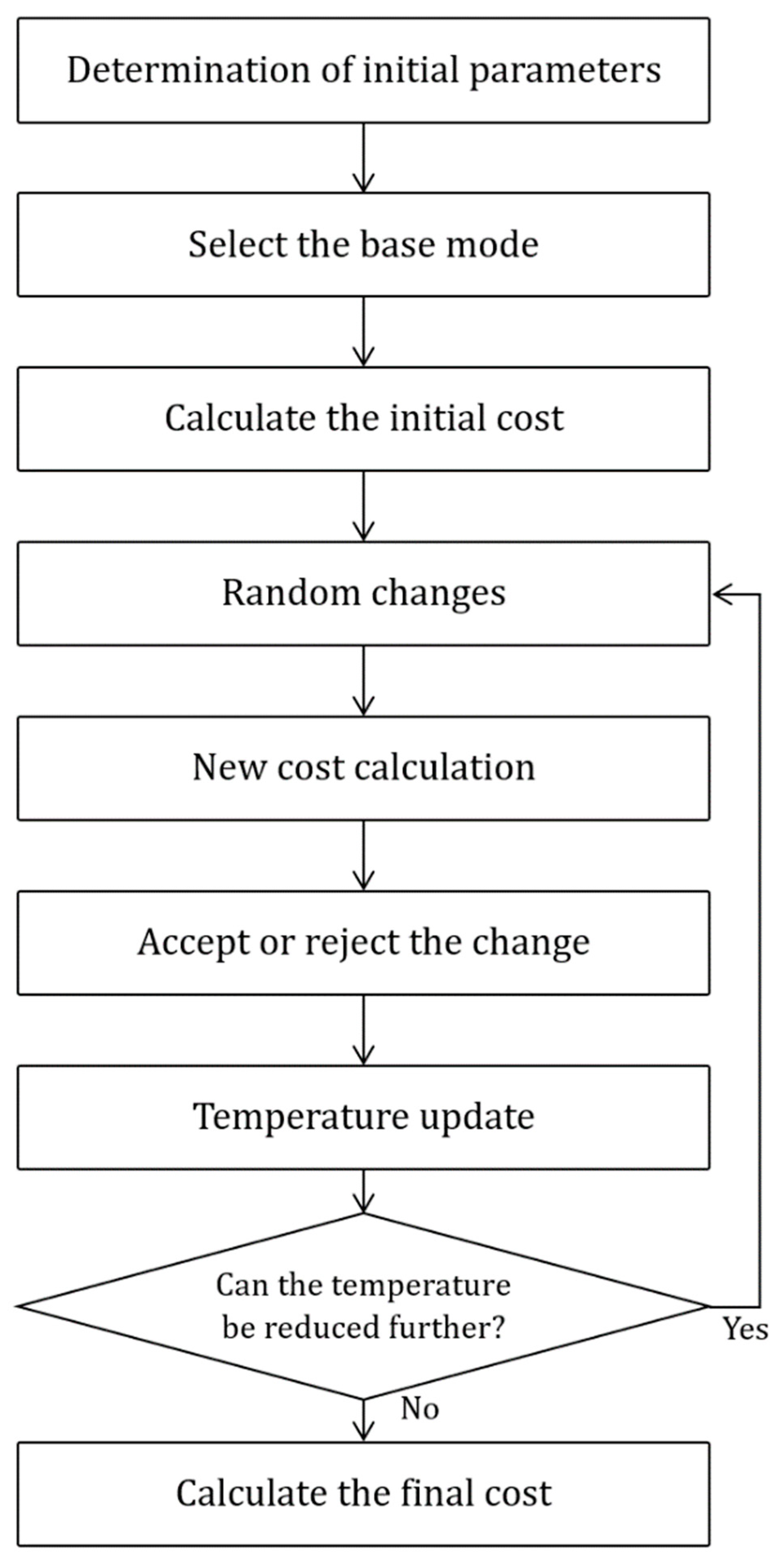
The steps of the SA algorithm for weight tuning in the XGBoost algorithm are as follows:

Setting Initial Parameters: The first step involves determining the critical parameters for the SA algorithm, including the initial temperature, cooling rate, and the number of iterations at each temperature. These parameters are chosen based on standard practices in similar studies and tailored to the problem’s complexity and the dataset’s characteristics. The initial temperature is set high enough to allow the algorithm to explore the solution space effectively in the early stages. The cooling rate is selected to ensure gradual convergence, balancing the trade-off between exploration and exploitation. The number of iterations at each temperature is determined to provide sufficient opportunities for evaluating potential improvements while maintaining computational efficiency. These parameters are closely tied to the model’s accuracy, influencing how well the algorithm navigates the solution space and identifies the optimal configuration for the XGBoost model.

Selecting Initial State: The XGBoost model’s initial state is chosen. This can include model parameters like tree depth, learning rate, etc., considered after training the initial and weak models, focusing on tree depths and their accuracies.

Calculating Initial Cost: The cost function for the initial state is computed.

Random Changes: In each iteration, a small and random change is applied to the current state to create a new state. It is important to note that random changes are only applied after completing the prerequisite steps, such as parameter initialization and initial cost calculation. These prerequisites ensure that the random changes are systematic and controlled, avoiding the introduction of any unstructured or unregulated influencing factors.

Computing New Cost: The cost function for the new state is computed.

Accepting or Rejecting Change: If the new state improves over the current state, it’s accepted. Otherwise, it might be accepted or rejected with a probability calculated based on the cost difference and the current temperature.

Updating Temperature: The temperature is updated using a cooling schedule to converge toward the optimal final state. This ensures the algorithm systematically moves towards an optimal solution while balancing exploration (through random changes) and exploitation (through temperature reduction).

Iteration: Steps 4 to 7 are repeated until the temperature reaches a certain low threshold or other conditions for algorithm termination are met.

Conclusion: The final state is presented as the optimal solution. To maintain the rigor and reliability of the optimization process, each step is systematically dependent on the outputs of previous steps, ensuring a clear and structured flow throughout the algorithm.

Figure 3 illustrates the flowchart of the proposed hybrid method for selecting the optimal combination of weights.

The advantages of this method compared to other approaches, as well as the straightforward XGBoost approach, are that parameter weight tuning in the algorithm occurs more accurately and effectively, minimizing the risk of getting stuck in local optima. On the other hand, by explicitly defining parameter weights in the algorithm, the final model’s accuracy also increases, leading to an improvement in the output quality.

3.3. The Validation Approach of the Developed Algorithm

For the development of the proposed models, 960 data records were used, with 75% designated for training data and 25% for testing data. This data split ratio is a common practice in the development of machine learning algorithms. This study was chosen due to the data volume and the relatively high number of features, ensuring that the model could be trained on an adequate amount of data. Additionally, allocating 25% of the data for testing allows a thorough evaluation of the model’s performance.

The data structure is such that values for all features are available for each data record, and the levels of uncertainty and complexity of the activity network are specified. Notably, all 960 data records were clean due to precise selection, with no outliers or noise among them. The dataset used includes several features with diverse ranges and characteristics. For instance, the number of activities averages 12.15, ranging from 6 to 25.5, while the number of critical activities averages 5.68, ranging from 2 to 20. The minimum and maximum duration of activities also show significant variation, with the minimum ranging between 20 and 30 days and the maximum ranging from 59 to 494 days. Other features, such as the number of contractors and the percentage of domestic versus foreign products, exhibit wide variability. The number of domestic contractors average 11.38, while foreign contractors average 4.87. Additionally, the percentage of domestic products is about 79%, with foreign products accounting for around 21%. Human resources vary between 31 and 189 individuals, and the estimated and predicted costs are in the billions, reflecting considerable differences across projects. This dataset provides comprehensive information on projects and contractors, highlighting notable variability in project complexity and resource allocation.

On the created dataset, first, the XGBoost algorithm was executed, and then the combined XGBoost—Simulated Annealing algorithm was developed. In the model validation section, the ANN, SVR, and DTR algorithms were also executed on the final dataset to provide a comprehensive comparison of the developed algorithm with other well-established algorithms in this field.

For the validation of the developed algorithm and the estimation of the desired error, performance metrics, including Accuracy, Precision, Recall, and F1-score, are employed [48,49]. Validation formulas of the developed algorithm are shown in relations (1)–(4).

$$Accuracy={\displaystyle \frac{{{\displaystyle \sum }}_{i=1}^{l}T{P}_i}{{{\displaystyle \sum }}_{i=1}^{l}T{P}_i+F{P}_i}}$$

(1)

$$Precision={\displaystyle \frac{{{\displaystyle \sum }}_{i=1}^{l}T{P}_i}{{{\displaystyle \sum }}_{i=1}^{l}T{P}_i+F{N}_i}}$$

(2)

$$Recall={\displaystyle \frac{{{\displaystyle \sum }}_{i=1}^{l}T{P}_i}{{{\displaystyle \sum }}_{i=1}^{l}T{P}_i+F{P}_i}}$$

(3)

$$F1-score={\displaystyle \frac{2\times \left(precision\times recall\right) }{\left(precision+recall\right)}}$$

(4)

where:

True Positive ($T{P}_i$): If the data actually has a $P_i$ label and the predicted value shows the same.

False Positive ($F{P}_i$): If the individual does not have a $P_i$ label, but the prediction result displays another label.

4. Definition of Features and Data Interpretation

This section interprets and analyzes the features and data used in the article. The article discusses constructing a model using 15 features, including project progress, number of activities, activity durations, network morphology, supplier counts, resources, and costs. It accounts for three types of uncertainties: project fundamentals, design and procurement, and project goals.

In this study, the dataset used for training the model and validation includes 960 records, covering a diverse range of construction projects. These projects vary in size and complexity. All the projects are residential, and the percentage of project progress is considered a feature for each project. Therefore, each project has various data points at different stages of progress. These projects also vary in budget, ranging from small residential projects to large infrastructure projects with much larger budgets. Geographically, the dataset includes projects from different regions, reflecting varying economic, regulatory, and environmental conditions. This diversity in the dataset ensures that the proposed model can be generalized across a wide range of real-world construction scenarios.

The features generally include the following:

-

Number of activities: Indicates the total activities involved in each project.

-

Number of critical activities: The number of activities that are critical for the project’s timely completion and cannot be delayed.

-

Minimum activity duration: The minimum time taken by any activity within the project.

-

Maximum activity duration: The maximum duration of any activity within the project.

-

The sum of activities morphology: The activities’ total morphological characteristics (likely structural features).

Uncertainty 1 Probability (Financial and Economic): The likelihood of encountering uncertainty in the project, with levels ranging from very low to very high. Uncertainty Type 1 relates to financial and economic uncertainties. Changes in exchange rates, sudden increases in raw material prices, fluctuations in labor costs, and market volatility are some factors that can affect the project’s budget and costs. This uncertainty can lead to changes in payment schedules or the need for additional financing.

Uncertainty 2 Probability (Technical and Design): This is another dimension of uncertainty, with values ranging from very low to very high. In construction projects, engineering designs may change or require revisions. This type of uncertainty includes inconsistencies in drawings, incomplete designs, or unforeseen technical issues. Additionally, issues related to material quality and the feasibility of executing the proposed designs can cause delays or project halts.

-

Uncertainty 3 Probability (Environmental and Natural Conditions): The third layer of uncertainty, characterized by levels ranging from very low to very high. Construction projects often face uncertainties due to natural and environmental conditions. Weather conditions (such as rain, snow, or storms), unforeseen geological conditions (like encountering unsuitable soil or underground water), and changes in environmental regulations can delay the project or necessitate rescheduling.

-

Number of domestic contracts: The number of contracts signed with domestic entities.

-

Number of foreign contracts: The number of contracts signed with foreign companies or partners.

-

Percentage of domestic production: The proportion of domestic production in relation to the project’s total output.

-

Percentage of foreign production: The share of production completed by foreign entities.

-

Human resources number: The total number of human resources or staff involved in the project.

-

Estimated cost: The project’s estimated cost is likely expressed in a specific currency unit.

Overall, the data structure indicates that projects with more “activities” and “critical activities” are likely more complex and require more careful management to avoid delays. Additionally, the “minimum activity duration” and “maximum activity duration” columns show the range of time required for each activity. A large difference between the minimum and maximum times may indicate variability in the complexity or dependency of the activities, which can affect scheduling. The uncertainty columns describe the project’s risk profile. If uncertainty is “very high,” the project will likely face significant challenges such as delays, increased costs, or resource shortages. Projects with lower uncertainty are likely more predictable. Overall, these features, along with network morphology characteristics, define the data analysis structure and the relationships between different variables.

A key feature is network morphology, highlighting the importance of activity interdependencies. The model addresses challenges in predicting project time, noting that neglecting network topology can lead to inaccurate forecasts. It contrasts serial and parallel network structures, emphasizing how the position and connections of activities impact project completion predictions. Therefore, this distinction among activity statuses in the project network should be considered when calculating indicators to obtain a more realistic picture of project execution and performance. Given the above explanations, in the proposed project indicators as dimensions of the project time prediction problem, three network morphology-related indicators are suggested:

-

The total number of activities in each project segment.

-

The number of critical activities in each project segment.

-

The minimum and maximum time among the activities in each project segment.

-

The innovation index to consider the network’s shape and the activity position.

In order to account for the project network shape and consider the positions of activities within the network. Initially, all paths in the project graph are calculated from the first node (project start) to the last node (project end). Then, for each individual project activity (nodes in the graph), it is determined how many of these paths exist. Finally, by dividing the number of paths in which activity i is present by the total number of paths in the network, an estimate of the completion time of the project is obtained. This yields a value between 0 and 1, representing the significance of the position of activity i within the project network and its relation to other activities. This indicator of network morphology is referred to as the “network morphology index” and is computed using Equation (5), where pi is the number of paths in the network where activity i is present, and p is the total number of paths in the network.

$$Network morfolog{y}_i={\displaystyle \frac{p_i}{p}}$$

(5)

Prior to constructing the predictive model, the relationships between features are first examined, and for this purpose, the Pearson correlation is utilized. Figure 4 illustrates the heatmap of the correlation coefficients among features.

For example, it is observed that there is a relatively strong relationship between the number of activities and progress. Additionally, these two features also have a strong and direct correlation with the number of domestic contractors, where an increase in these factors significantly impacts the project’s progress. The number of domestic contractors has the most substantial influence on predicting both cost and time, highlighting the importance of this feature. Another noteworthy point is that the percentage of foreign products has a significant impact on the number of critical activities, as well as the project costs and time. This indicates that utilizing domestic contractors and products, which can be more readily supplied from various aspects, can significantly affect the project’s time and cost.

For example, the number of activities has a strong correlation with project progress. In other words, the relationship between critical activities and the total number of activities is also significant. On the other hand, a notable correlation exists between activities and external contracts and estimated costs, which is natural. These relationships essentially validate the relevance and logic of the identified features.

To ensure that the correlation between certain features does not affect the developed model, a Variance Inflation Factor (VIF) analysis was conducted. It is important to note that the algorithm used in this study, XGBoost, operates based on tree structures and inherently has the capability to handle multicollinearity. A VIF value below 5 indicates no issue, while a value between 5 and 10 suggests moderate multicollinearity and values above 10 indicate severe multicollinearity. The VIF calculation for the features showed that the activities number and percentage of domestic products had values in the range of 8–9. However, given the low VIF values for the other features and the use of the XGBoost algorithm, this does not pose a significant issue.

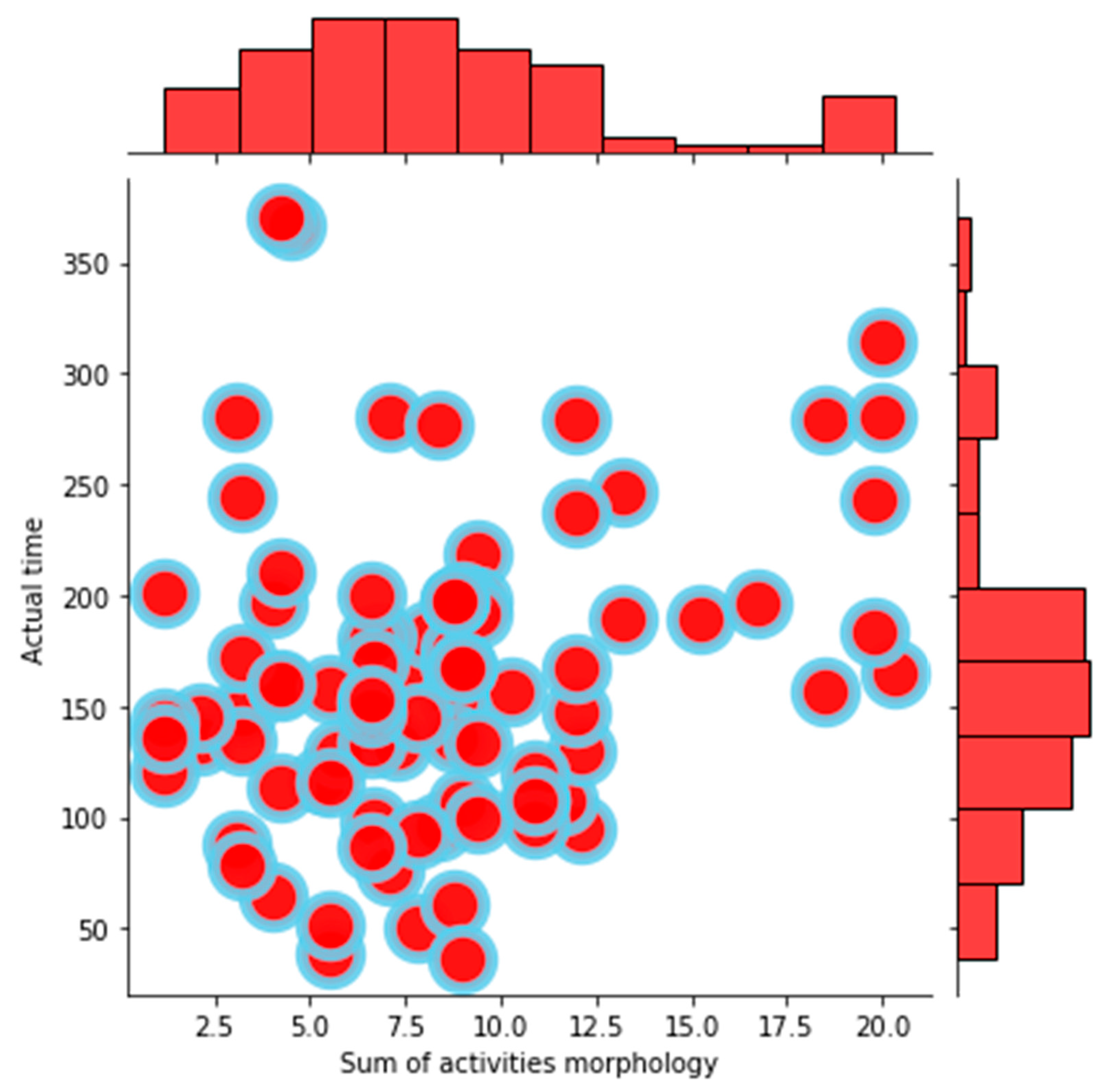
Another crucial component in the current paper’s model is the morphological network feature. Figure 5 illustrates the impact of the number of activities and critical activities on this feature. It can be seen that as the number of activities and critical activities increases, this feature also exhibits an increment, thus affirming the credibility of the proposed indicator.

5. Result

This section reports the article’s findings. First, the time and cost prediction model is developed, followed by its validation and comparison with conventional approaches for time and cost estimation and prediction. Finally, sensitivity analysis and managerial insights are presented.

5.1. Developing a Time and Cost Forecasting Model

To construct the prediction model for time and cost, initially, using the XGBoost algorithm and the data described in the previous section, predictions were made for cost and time. An important point to note is that the Hessian matrix approach was employed in the weight-tuning step within the XGBoost algorithm. However, this approach might lead to the problem converging to a local optimum, failing to achieve the best solution. On the other hand, the values of Accuracy, Precision, Recall, and F1-score metrics for the designed model were calculated as 0.869, 0.891, 0.910, and 0.871, respectively. The SA algorithm is then used to enhance the model’s accuracy.

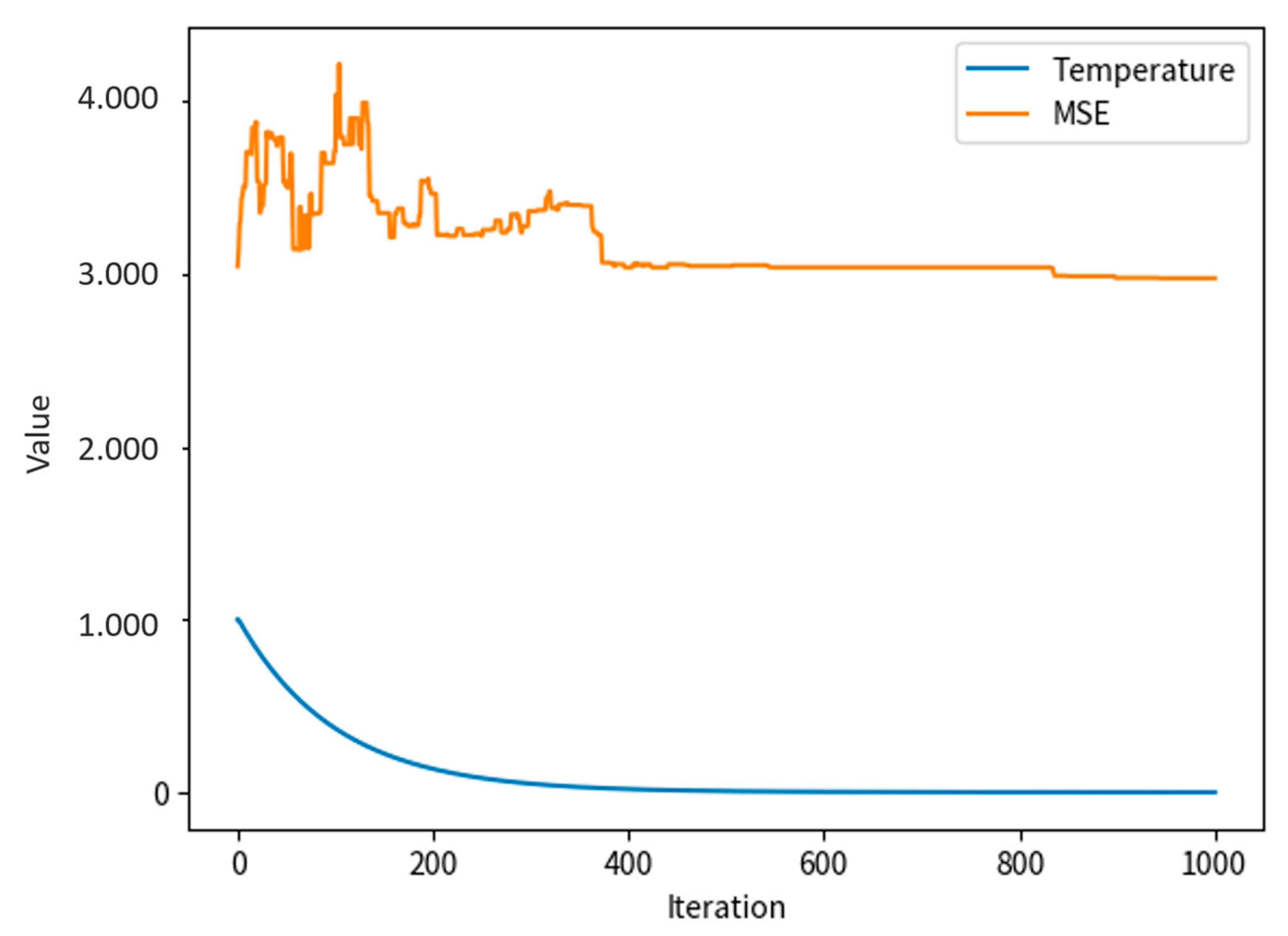
In this regard, to execute the XGBoost algorithm in conjunction with SA, the initial values of the weights, or in other words, the temperature, were determined. The algorithm was then iterated several times, with the initial weights randomly selected. The error values were calculated using the Boltzmann function, and the selected values were determined, updating the weights accordingly. The temperature decreases with a predefined rate by identifying the optimal weights, and the final weights, along with the optimal error, are selected.

One of the challenges in implementing the SA algorithm is the number of iterations. Iteration refers to a step or repetition. In each iteration, the algorithm introduces a small weight change and decides whether to accept or reject this change.

The number of iterations is one of the parameters of the algorithm and can significantly impact its efficiency and results:

-

If the number of iterations is too small, the algorithm might get stuck in a local optimum and fail to reach the global optimum.

-

If the number of iterations is too large, the algorithm might require a long execution time.

In the algorithm executed for values ranging from 1 to 1000 iterations, as depicted in Figure 6, the MSE and temperature values reach their lowest point after 380 iterations.

On the other hand, as illustrated in Figure 7, the performance of the model on the initial test set is also reasonable and acceptable (R² = 0.699). The XGBoost-SA model can be considered as a reference model for predicting cost and time.

5.2. Validation of the Developed Algorithm

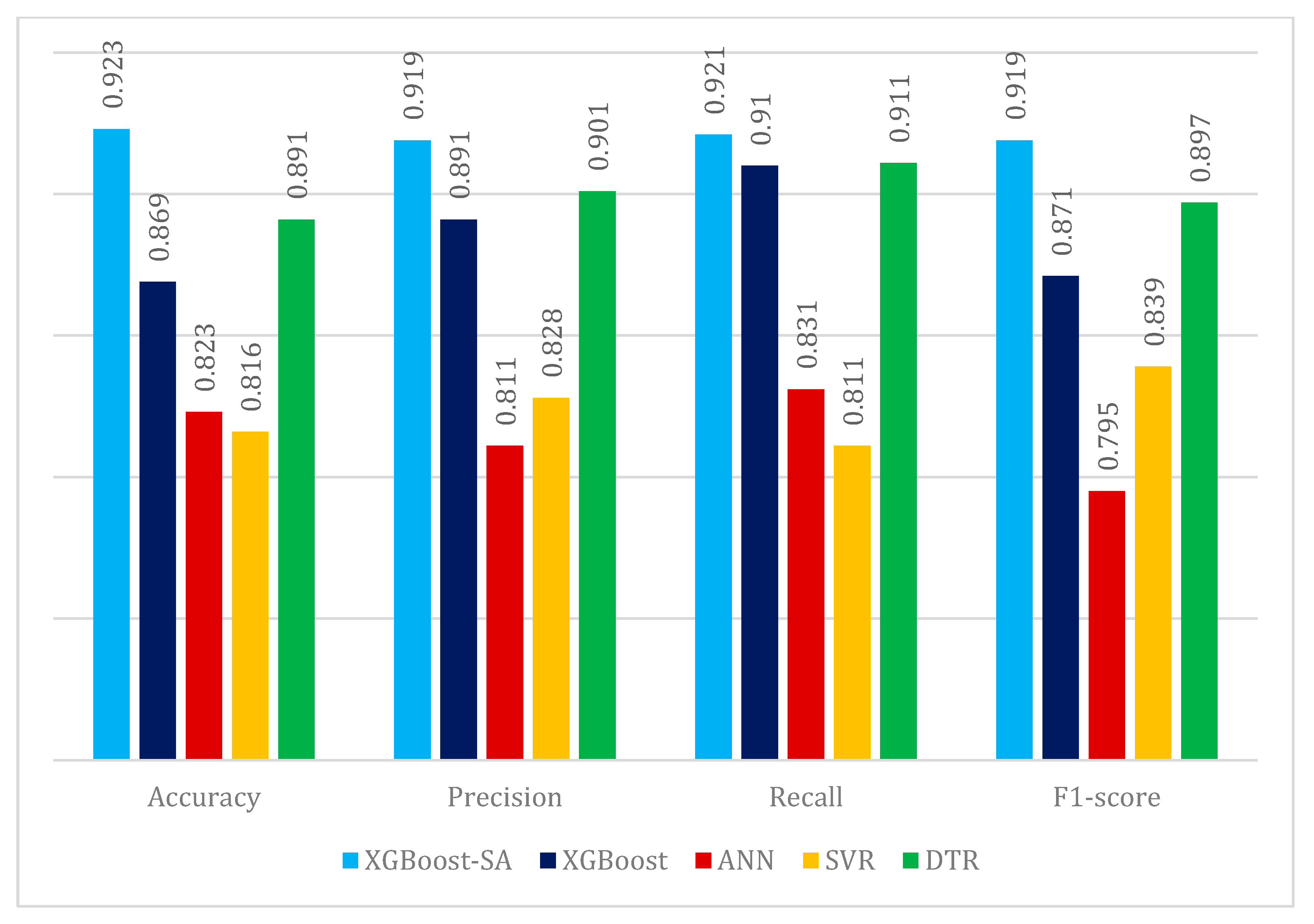
To evaluate the developed model and compare it with other machine learning algorithms in this field, four metrics based on Equations (1)–(4) are employed. In this regard, the algorithm proposed in this paper is compared with XGBoost, Artificial Neural Network (ANN), Support Vector Regression (SVR), and Decision Tree Regression (DTR) algorithms, as shown in Figure 8. As a neural network-based and black-box method, ANN demonstrates the model’s ability to handle non-linear and high-dimensional relationships. As a kernel-based method, SVR performs well in solving both linear and non-linear problems, making it highly suitable for comparison. On the other hand, DTR, a tree-based algorithm, provides interpretable results and shares a similar foundation with XGBoost. The selection of these algorithms facilitates a comprehensive comparison of the proposed method with various structures of machine learning algorithms.

According to Figure 8, the XGBoost-SA algorithm has exhibited significantly better performance in the evaluation metrics. Tree-based algorithms such as DTR, XGBoost, and the enhanced XGBoost with SA perform better than other algorithms. Therefore, the use of tree-based algorithms in predicting cost and time demonstrates superior efficiency and performance.

5.3. Feature Importance in Time and Cost Prediction

In this section, the feature importance has been calculated. In the XGBoost algorithm, it is possible to compute feature importance using various methods. In this model, Gain (Information Gain) has been used, which is calculated according to Equation (6).

$$Gai{n}_i={\displaystyle \frac{{\mathrm{Total} \mathrm{Gain} \mathrm{from} \mathrm{Splits} \mathrm{Using} \mathrm{Feature}}_i}{{\mathrm{Number} \mathrm{of} \mathrm{Splits} \mathrm{Using} \mathrm{Feature}}_i}}$$

(6)

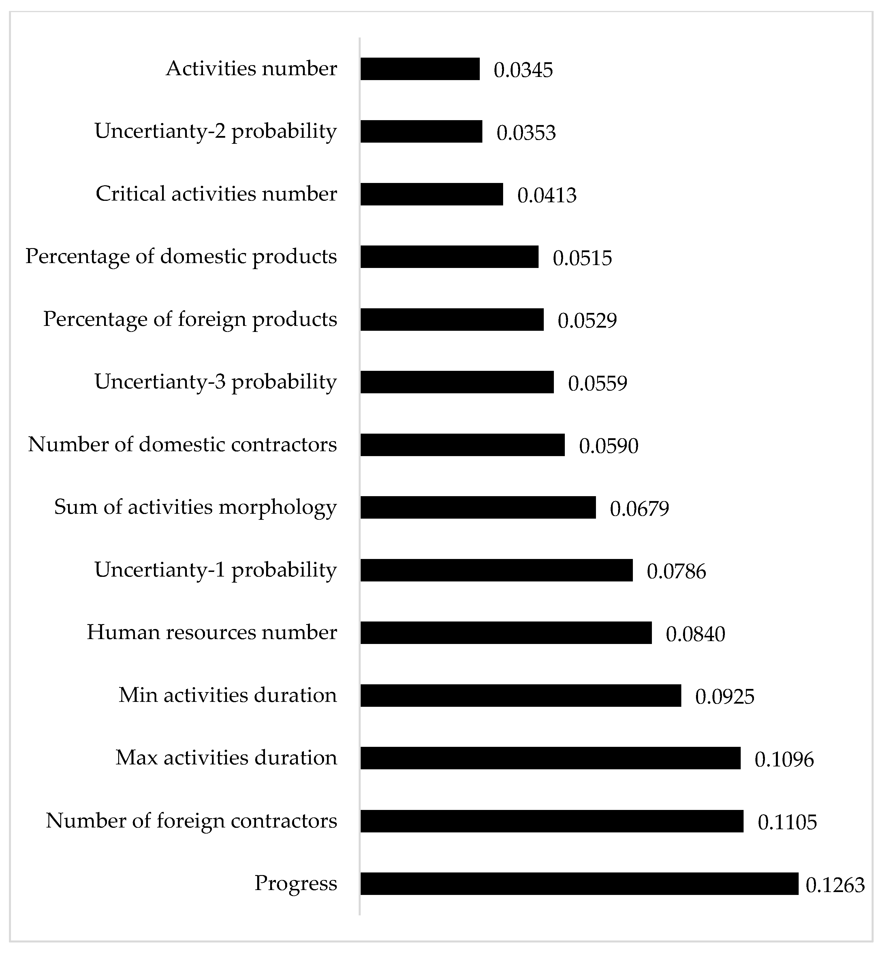
The Gain metric measures the reduction in error (Mean Squared Error, MSE) achieved by splitting a node using a particular feature. If a feature significantly reduces the error, it has a higher value in the model. As illustrated in Figure 9, the feature’s importance is presented. It can be observed that Progress holds the highest importance, and among the uncertainties, Type 1 has the most influence on predicting time and cost. Additionally, the number of human resources and foreign contractors also shows a greater impact compared to other features. However, it is noteworthy that all features hold considerable importance, which highlights the appropriate selection of features in the model development process.

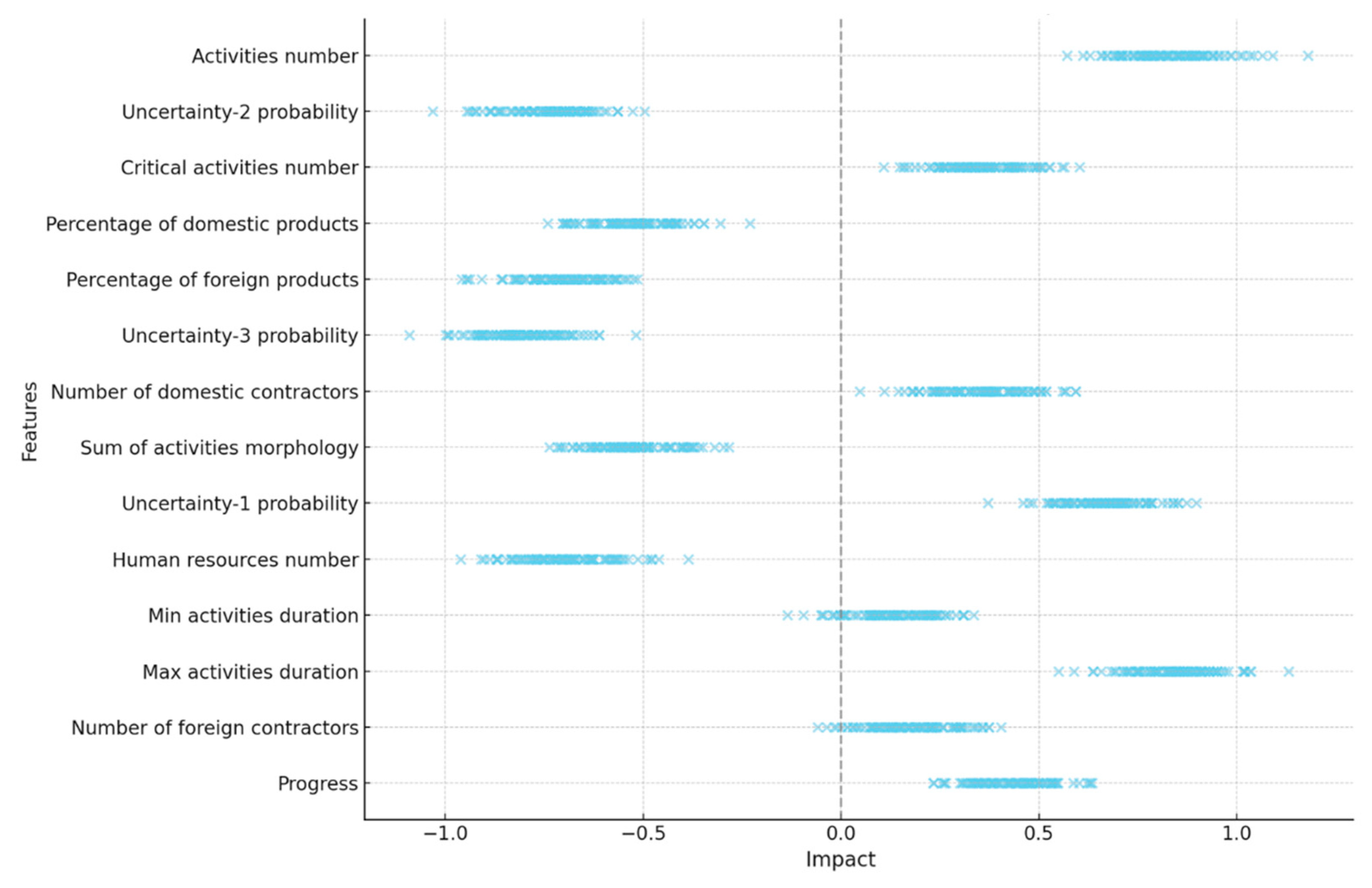
Additionally, to better interpret the features and their impact on predictions, the SHAP Beeswarm plot has been utilized. This visualization tool is designed to interpret machine learning models by showing how each feature affects the model’s predictions. Figure 10 presents the SHAP Beeswarm plot for the features of the model used in this study. The vertical axis displays the features ranked by importance, while the horizontal axis represents the impact of each feature on the model’s output. According to the findings in Figure 10, the feature Progress not only plays a key role but also shows varying impacts depending on the input data, being positive in some cases and negative in others. Furthermore, features such as the Activity number, Max activities duration, and Uncertainty type 2 and type 3 have significant influences on the predictions.

5.4. Comparison of the Article Model with Other Forecasting Approaches

In this section, a comparison between three models for predicting project execution time and cost is presented, including the XGBoost-SA model and the traditional models ESM (Earned Schedule Method) and EVM (Earned Value Management). ESM and EVM are two traditional approaches for predicting project costs and duration. These models operate based on specific and fixed formulas and do not rely on the interdependencies between variables or learning from past data. These models often estimate time and cost based on the current project trend without considering historical data or the complex interactions between variables. The XGBoost-SA model used in this comparison is a machine learning-based model that can account for the complex relationships and dependencies between various variables. This model utilizes past data for learning and optimizing predictions, allowing it to perform more accurately in many cases than traditional models.

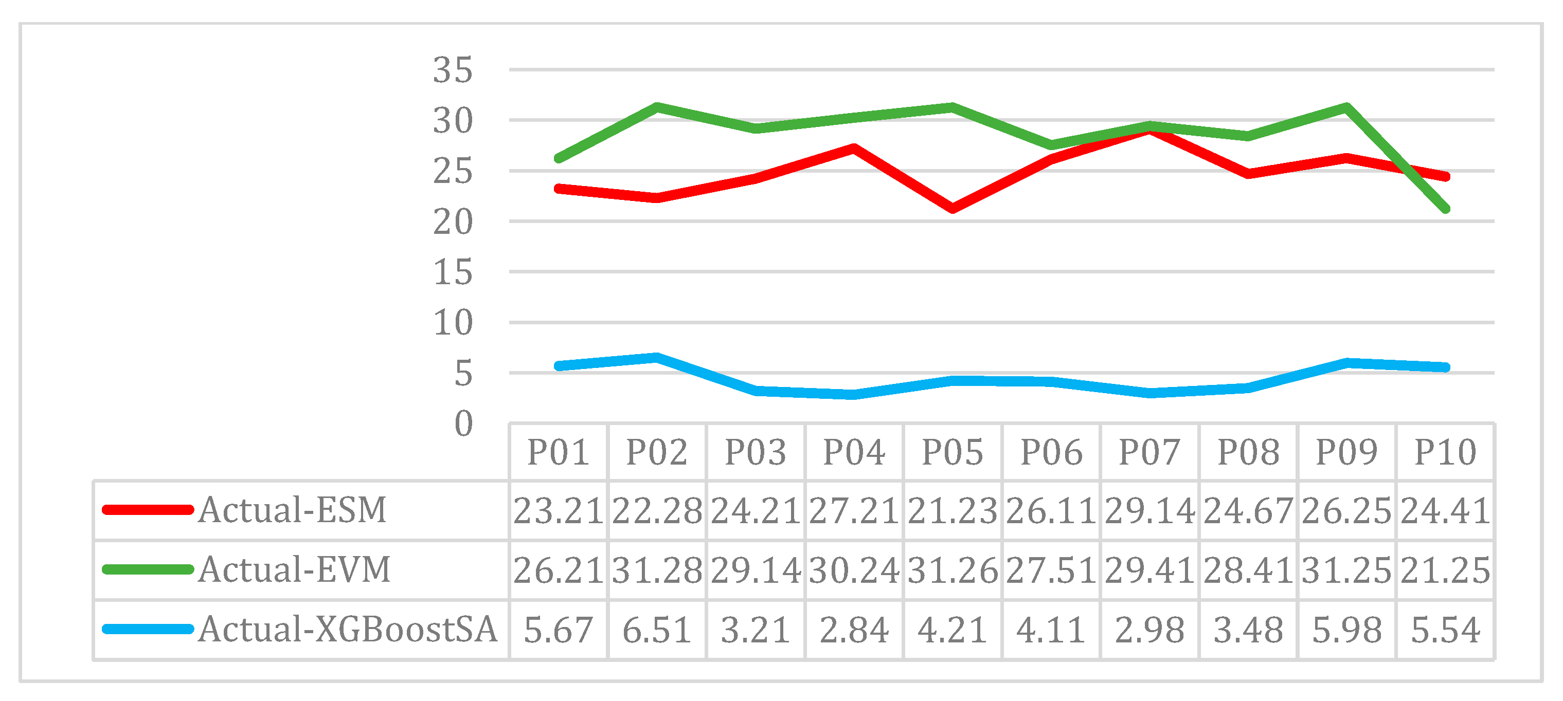
In Figure 11, a comparison is made between the predictions of each of these models for the execution time of 10 different projects. The data in the table associated with this figure shows that the XGBoost-SA model is significantly more accurate in predicting time than the traditional ESM and EVM models. For example, in project P01, the ESM model predicted a time 23.21% higher than the actual value, while the EVM model predicted a time 26.21% higher than the actual value. In contrast, the XGBoost-SA model only had a 5.67% difference from the actual value. In other projects, it is also evident that the XGBoost-SA model generally has a smaller margin of error than the actual values, indicating that it provides more accurate project time predictions.

In Figure 12, the results related to the prediction of project costs are shown. The chart in Figure 11 examines the percentage difference between actual costs and predicted costs for ten projects using each method. For example, in project P01, the ESM model predicted a cost 13.54% higher than the actual value, the EVM model predicted a cost 11.25% higher than the actual value, while the XGBoost-SA model had only a 7.41% difference from the actual cost. This trend is also observed in other projects. For instance, in project P04, the ESM model had a 16.74% difference, and the EVM model had a 17.51% difference compared to the actual costs, while the XGBoost-SA model showed only a 4.11% difference.

Based on the data and results from both figures, it can be concluded that the XGBoost-SA model performs better in predicting project time and cost compared to the traditional ESM and EVM models. This can be attributed to the fact that XGBoost-SA utilizes historical data to improve the accuracy of its predictions and takes into account more complex relationships between variables. In contrast, ESM and EVM models, due to their use of simplified approaches and lack of learning from past data, cannot achieve the same level of prediction accuracy. Overall, the use of machine learning-based models like XGBoost-SA has increasingly proven to be more practical for predicting project costs and durations. These models are capable of reducing prediction errors and delivering more accurate results compared to traditional methods, especially in complex projects where multiple factors influence their success.

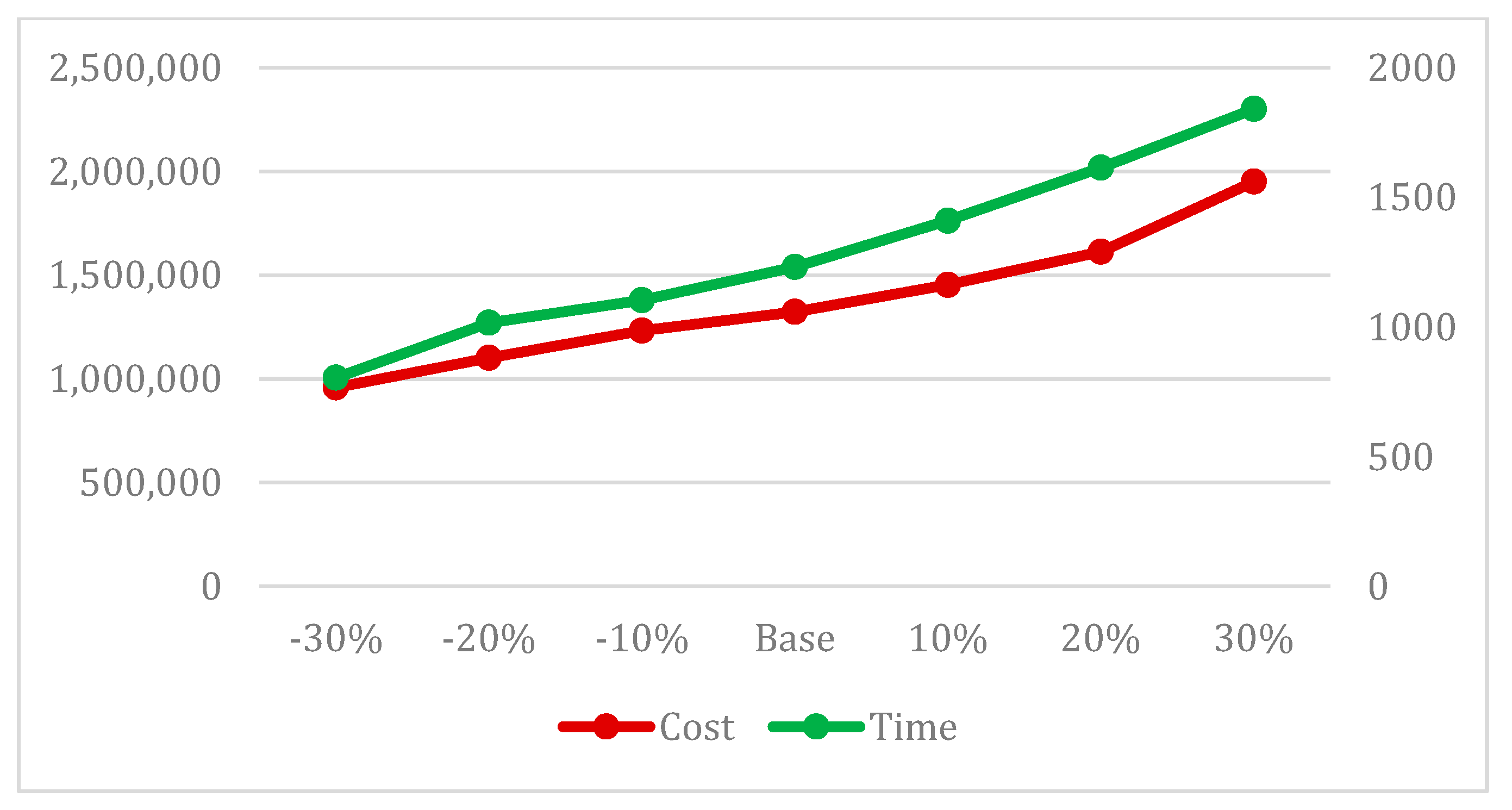
5.5. Sensitivity Analysis

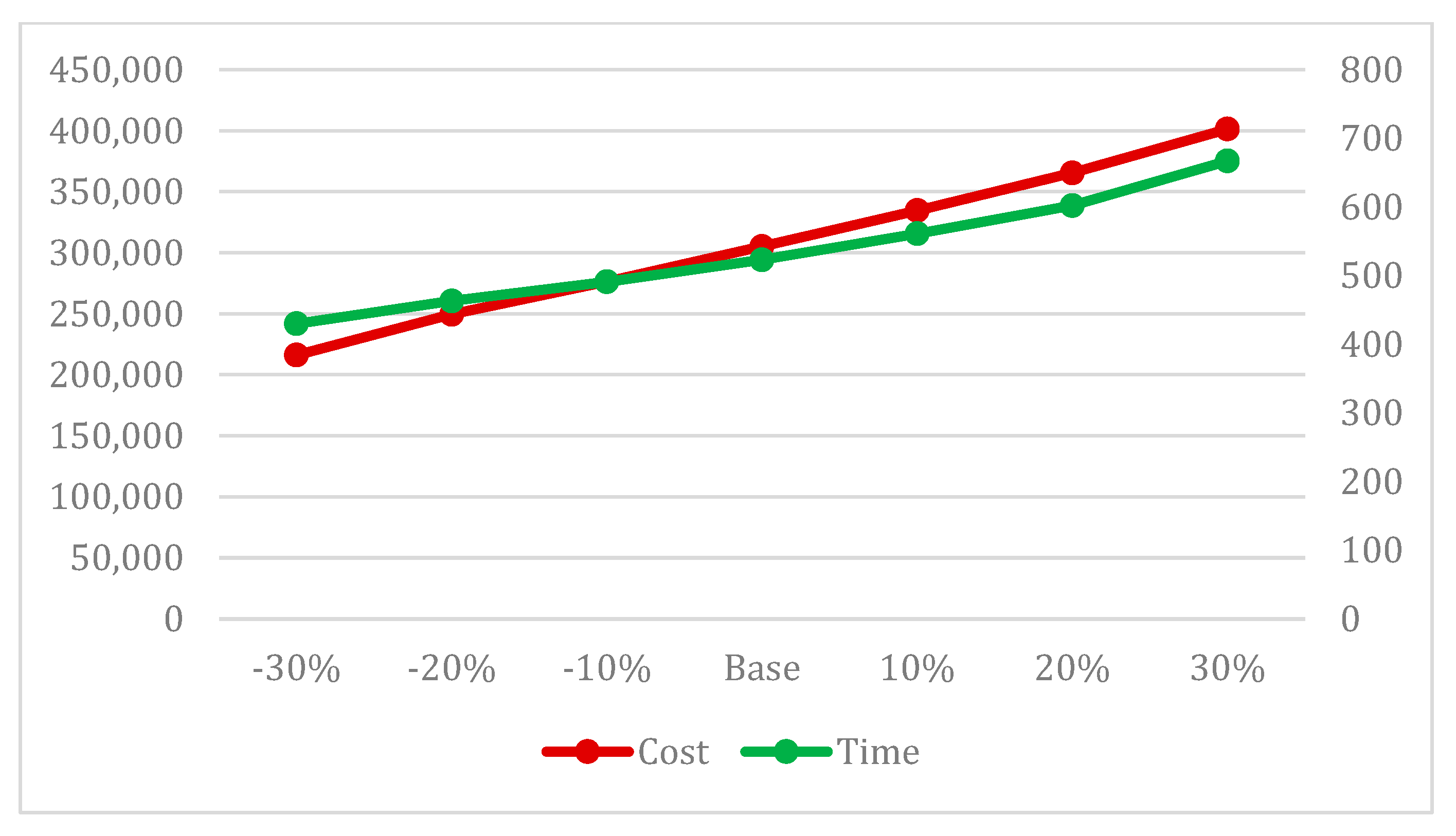
In this section, the sensitivity of the target values, the project completion time, and cost to the critical indicators specified in this article and the examined model is evaluated by varying the values and probabilities associated with uncertainties and project complexities. Figure 13 demonstrates that as the level of uncertainty increases or decreases, the project completion time and cost also increase or decrease, indicating the correct algorithm performance concerning this indicator. Furthermore, Figure 14 also illustrates that the project completion time and cost change with variations in the complexity of the project network. Additionally, in Figure 15, the simultaneous impact of uncertainty and complexity on time and cost has been analyzed, demonstrating greater deviations and variations. This highlights the accurate performance of the model.

5.6. Managerial Insight

The results obtained from comparing the XGBoost-SA algorithm with traditional models such as ESM and EVM demonstrate that this algorithm performs better in predicting project time and cost. Since the XGBoost-SA model utilizes historical data and machine learning to analyze complex relationships between variables, it can provide more accurate predictions than traditional models. In contrast, due to their reliance on simplified approaches and lack of leveraging past data, ESM and EVM models have limitations in managing complex projects that involve high levels of uncertainty and complexity.

The key benefits of the XGBoost-SA model for project managers can be summarized as follows:

-

More accurate time and cost prediction: The use of the XGBoost-SA model helps project managers predict project completion time and costs with greater accuracy. This higher level of accuracy, especially in complex projects, prevents incorrect decision-making and avoids additional costs.

-

Better risk and uncertainty management: The XGBoost-SA model can account for various uncertainties, such as price changes, technical issues, and environmental conditions. This enables project managers to anticipate risks in a timely manner and adopt more effective strategies to manage them.

Faster decision-making: The XGBoost-SA model’s faster processing and higher accuracy allow project managers to respond more quickly to changing project conditions, improving the decision-making process and reducing delays.

-

Utilization of historical data for project optimization: One of the key features of the XGBoost-SA model is its ability to use past data. Managers can analyze historical data from similar projects to make better predictions and more precise planning, leveraging past experiences to optimize new projects.

-

Reduction in prediction errors: This model significantly reduces prediction errors, allowing managers to manage project resources more effectively and prevent wastage of time and budget.

Overall, the XGBoost-SA model helps project managers make better decisions and provides higher accuracy in predicting time, cost, and risk management. Using these data-driven models enhances project efficiency and mitigates potential problems arising from uncertainties and unforeseen changes.

5.7. Practical Implications

This model enhances project management by providing highly accurate predictions for completion times and costs, achieving over 92% accuracy. It aids in resource optimization by aligning staffing needs precisely with project demands, preventing waste. The model also supports effective risk management by accounting for uncertainties and task interdependencies, proactively mitigating delays and cost overruns. Additionally, it boosts stakeholder confidence through reliable outcome predictability and robust control of milestones and budgets. The model’s accurate predictions support strategic decision-making, helping managers align resources with organizational goals. Its adaptability allows for quick responses to changes, enhancing flexibility in project execution. The model is valuable for implementing performance-based pay systems and planning new government projects, promising improved performance and service delivery.

6. Conclusions

For the first time, this article introduces the XGBoost-SA algorithm for estimating and predicting project completion time and cost. While the XGBoost algorithm is particularly effective when working with small to medium data volumes due to its efficiency and low computational overhead, it also demonstrates scalability and adaptability for larger datasets. This makes it suitable for various applications, including complex, data-intensive projects. Compared to algorithms like ANN and SVR, XGBoost consistently performs better in predicting time and cost, with results similar to DTR’s. However, the developed XGBoost-SA algorithm surpasses these methods due to its precise optimization using Simulated Annealing, achieving over 92% accuracy in predictions. Furthermore, this algorithm significantly outperforms traditional methods like ESM and EVM, reducing cost prediction errors by half and time prediction errors by approximately one-fifth.

In conclusion, this study’s findings underscore the XGBoost-SA model’s superiority over traditional approaches in predicting project time and cost. The XGBoost-SA model effectively addresses complex and nonlinear relationships between project variables by leveraging historical data and advanced machine learning techniques and offering a robust and accurate prediction framework. This model equips project managers with essential tools for informed decision-making, enabling them to anticipate risks, manage uncertainties, and optimize resources efficiently. Its capacity to incorporate lessons from historical data further reduces prediction errors and minimizes costs. The XGBoost-SA model’s ability to handle high complexity and uncertainty makes it exceptionally valuable for managing large-scale and intricate projects. Adopting data-driven models like XGBoost-SA enhances project efficiency, reduces delays, and provides a strategic advantage in modern project management.

The use of data-driven algorithms, particularly hybrid approaches combining machine learning with metaheuristic and optimization methods, continues to draw significant attention across various research domains. This study highlights the potential for such combinations to enhance prediction accuracy. However, a fundamental limitation remains the availability of sufficient data, underscoring the need for researchers to focus on comprehensive data collection to enable the development of robust machine learning models.

For future research, we recommend optimizing the XGBoost algorithm with methods such as Genetic Algorithms and Particle Swarm Optimization (PSO) and comparing their performance with this study’s findings. Additionally, testing the XGBoost-SA algorithm on larger datasets and applying it to industries such as telecommunications and startups could provide further insights into its versatility. Exploring the effects of increasing iterations or modifying the cooling schedule in the Simulated Annealing process could also enhance the algorithm’s performance.