Dynamics and Chaos Intensity Analysis of Under-Actuated Mechanism by Uniformity and Particle Swarm Optimization

Abstract

Generally, nonlinear systems have dynamic uncertainties, and under certain conditions, the systems exhibit different chaos intensities. Therefore, it is an important consideration for designers to realize the suppression and enhancement of chaos intensity under nonlinear factors according to the actual situation, but there are few research results on this problem. To investigate the dynamic performance and chaotic intensity of a nonlinear mechanism, a planar closed-chain under-actuated mechanism, which has not been extensively studied before, is taken as an example. It is worth noting that a small change in the parameters of a nonlinear system will cause a large change in the motion state of the system and even the mutual transformation between chaotic phenomena and periodic phenomena. To solve this problem, uniformity is used to evaluate the chaos intensity of the system. Finally, based on uniformity, the particle swarm optimization algorithm successfully achieves the suppression and enhancement of the chaos intensity of the closed-chain under-actuated five-bar mechanism by optimizing its linkage length and driving speed, and the results are verified by the experimental platform.

1. Introduction

Chaos phenomena are wide-spread in nonlinear mechanical systems, such as gear systems [1], cam-follower mechanisms [2], rigid–flexible mechanisms [3], parallel mechanisms [4], planar mechanisms [5], under-actuated systems [6], and others [7,8]. In these areas of research, dynamic analysis and force analysis in a chaotic state are current hot spots [9,10,11]. However, there is little research on how to evaluate the chaos intensity of a system and realize the change in the chaos intensity of the system through a small change in the parameters of the mechanism, so that the chaos intensity and motion state of the mechanism can meet the actual needs. This paper mainly analyzes the dynamic modeling of under-actuated mechanisms, the influence of the driving speed and linkage length on the chaos intensity, and the optimization of the chaos intensity based on particle swarm optimization (PSO).

To improve the performance of a nonlinear system, many scholars use optimization [12], parameter design [13], force analysis [14], control [15,16], external disturbance [17], and other methods [18,19]. In the meantime, the majority of these works have concentrated on mathematical modeling and numerical simulation of the system’s dynamic behavior, so that a great deal of work has been conducted in this field [20,21]. In general, chaos control and force control of nonlinear mechanisms are realized by changing the size of clearance, driving speed, and joint friction in the mechanism with clearance, which is the main research method at present [22,23]. In these studies, some relatively novel methods are also used. To achieve the suppression of chaos intensity, Wu et al. [24] successfully suppressed the chaos intensity of a system under various parameters by adjusting the vibro-impact oscillator of the planar slider mechanism with a clearance joint. Arian and Taghvaei [25] mainly studied the modeling and analysis of chaotic dynamics of spur gear transmission systems with an idler and controlled the range of strange attractors of the system through the idler to achieve the suppression of chaotic phenomena of the system. In order to achieve chaos control of the pendulum, Kudra et al. [26] successfully achieved the goal of chaos suppression of the pendulum by installing a DC motor on the slider and using a phase diagram and bifurcation diagrams at the same time. To determine the parameter conditions of the transformation between chaotic motion and periodic motion in nonlinear systems, Li et al. [27] analyzed the motion states of the closed-chain under-actuated five-bar mechanism under different driving speeds and linkage lengths using permutation entropy and the Lyapunov exponent. This is also a reliable way to control the chaos of the system by changing the position of the center of mass of the linkage mechanism and changing the moment of inertia of the system [28,29].

Synthesizing the above studies, the mechanism chaos phenomena in nonlinear mechanisms have been analyzed widely, but there are few studies on how to judge the chaos intensity. Therefore, the main goal of this paper is to conduct a study on chaos intensity; thus, uniformity is chosen. Uniformity theory is a new conception proposed by the Chinese scholar Chuanwen Luo [30]. This theory focuses on describing the degree of dispersion of limited data within predefined boundaries, as well as the degree of spatial separation between points. Although this theory has the advantage of chaotic intensity judgment, it has not attracted the attention of scholars. To illustrate the correctness of uniformity, the bifurcations of logistic mapping and the Duffing oscillator are used, and the results prove that uniformity can be used to judge the chaos intensity.

According to the research results of previous scholars, the chaotic state of a nonlinear mechanism system can be transformed by changing the structural parameters of the system, such as the driving speed, the size of the clearance joints, and the force of the joint. Inspired by the above methods, this paper changes the chaos intensity of the system by changing the linkage length and drive speed of a closed-chain under-actuated five-bar mechanism. Compared with the common chaos caused by a clearance joint, the chaos caused by an under-actuated mechanism is more controllable, has a smaller impact force, and leads to less joint wear [27]. However, there is little research on the chaos phenomena caused by under-actuated mechanisms, which is mainly in the theoretical research stage at present, and the utilization of its chaos intensity will be the research focus at a later stage. Therefore, the main objective of this article is to establish a correct dynamic model of a closed-chain under-actuated five-bar mechanism and analyze the chaos intensity of the system through uniformity. In the last section, based on the uniformity theory and PSO, the chaos enhancement and suppression of the closed-chain under-actuated five-bar mechanism under certain conditions are successfully realized by optimizing the length of the linkage. This conclusion is also verified by the experimental platform.

2. Theoretical Framework of Uniformity and Examples

In Euclidean n-dimensional space, suppose $S$ is a finite set in ${\mathbb{R}}^{\mathrm{n}}$; let $x\in S$, $y\in S$, and $y\ne x$. If $A$ is simply connected and $S\subset A$, and the polyhedron $A$ is considered to be the boundary polyhedron of $S$, then denote $V^{*}$(●) as capacity and ${\mathrm{V}}^{*}$(A) = $A_v$. Use M(x) = mid (x, y) to represent the minimum distance between two Euclidean points. By denoting $M\left(x\right)={min}_{y\in S,y\ne x}d(x,y)$, the proximity distance is expressed by $M\left(x\right)$. A space sphere, whose center point is $\mathrm{x}$ and radius is $M\left(x\right)/2$, is called the monopolized sphere, which is expressed as $B\left(x\right),$ and its volume is $v\left(x\right)$.

The volume of the space sphere is

$$V_n(r)={\pi }^{n/2}{r}^n/\Gamma ({\displaystyle \frac{n}{2}}+1)$$

(1)

where $\Gamma \left(\mathrm{x}\right)$ is the $\Gamma$-function, and n = 1, 2, …, r is the radius of the space sphere.

By substituting $r=M\left(x\right)/2$ in Equation (1), we obtain the following:

$$v(x)=V_n[{\displaystyle \frac{M(x)}{2}}]={\displaystyle \frac{V_n(1)}{2^n}}M{(x)}^n$$

(2)

where $V_n\left(1\right)$ is the volume of the unit sphere in ${\mathbb{R}}^{\mathrm{n}}$.

Let $S$ have k points; then, the entire monopolized sphere volume, $a$, in $S$ is

$$a={\displaystyle \sum _{i=1}^k{V}^{*}}(B(x_i))={\displaystyle \sum _{i=1}^{k}v(x_i)}$$

(3)

There are many n-dimensional cubes with the monopolized sphere as the inner sphere, but their volume is the same. Choosing any n-dimensional cube as the monopolized body of $x$, its volume $vc\left(x\right)$ is

$$vc(x)=M{(x)}^n=2^{n}v(x)/V_n(1)$$

(4)

Then, the uniformity (L) is

$$L(k)=2^{n}a/[V_n(1)A_v]=2^n{\displaystyle \sum _{i=1}^{k}v(x_i)}/[V_n(1)A_v]={\displaystyle \sum _{i=1}^{k}vc(x_i)}/A_v={\displaystyle \sum _{i=1}^k{M}^n}(x_i)/A_v$$

(5)

Additional instructions for Equations (1)–(5) are as follows:

(1) If n = 1, the monopolized sphere should be called the monopolized line, and if n = 2, the monopolized sphere should be called the monopolized circle.

(2) The points in $S$ are finite and non-coincident, the monopolized spheres are only tangential or separated from each other, and there is no intersection.

(3) The range of uniformity, L, is (0, 1); a bigger value of L means a more discrete distribution of points in ${\mathbb{R}}^{\mathrm{n}}$.

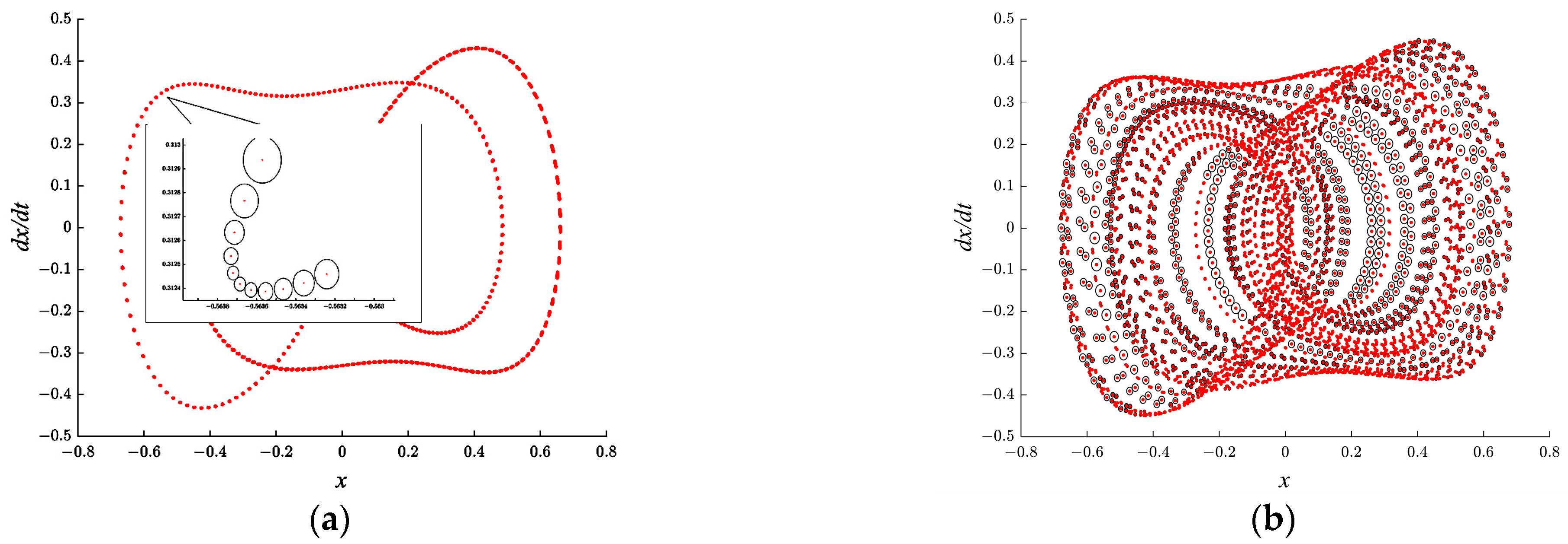
An example of different values of L with the same data points is shown in Figure 1.

The number of points in Figure 1 is 4000; the red dots represent the position of the points in the phase portrait, and the black circles represent the monopolized circles. The points in Figure 1a are more concentrated and have a smaller value of L of 0.00014, while the data in Figure 1b are more divergent and have a larger value of L of 0.1469. The results in Figure 1 show that under the condition of the same points, the degree of dispersion of data points will affect the chaos intensity of the system, and the value of L can evaluate its intensity.

2.1. Logistic Mapping Example

The logistic mapping equation is

$$x_{n+1}=k{x}_n(1-x_n)$$

(6)

where n = 0, 1, 2, …, k is the system parameter.

Let $x_0$= 0.1; the simulation step size is 0.005, and iteration occurs every 2000 steps. The bifurcation diagram and L of the logistic mapping are shown in Figure 2.

In Figure 2, when the data points in Figure 2a change from one status to another, e.g., k = 3.83, the status changes from chaotic motion to periodic motion; meanwhile, in Figure 2b, L diminishes immediately. By comparing Figure 2a,b, it can be seen that when the system is in a state of periodic phenomena, the value of L is small and approaches 0, while when the system is in a state of chaotic phenomena, the value of L is large. The value of L in Figure 2b is consistent with the distribution of the bifurcation diagram points in Figure 2a, which indicates that the value of L can reflect the chaos intensity of the system.

2.2. Duffing Oscillator Example

The Duffing oscillator equation is as follows:

$$\left\{\begin{array}{l}\dot{x}=y\\ \dot{y}=-ry+kx-s{x}^3+F\cos (t)\end{array}\right.$$

(7)

where t is the time; F is the excitation amplitude; and r = 1, k = 1, and s = 5.

Let 0.2 ≤ F ≤ 1 and let its value increase by 0.002 each time; the initial values of x and y are set to 0, the simulation step of t is $\mathsf{\pi }$/50, and its period is $\mathsf{\pi }$. According to the initial values of x and y, and using Equation (7), the bifurcation diagram of the Duffing oscillator is obtained by using the Runge–Kutta method in MATLAB, as shown in Figure 3.

It can be seen from Figure 3 that the Duffing oscillator has multiple regions of single and multiple periods, and it alternates between periods and chaos. Within the chaotic interval of logistic maps, L is greater than zero, and the maps increase or decrease at almost the same time. Both Figure 2 and Figure 3 show that the value of L can reflect the chaos intensity.

Further analysis of Figure 3b reveals that uniformity has successfully monitored the variation in chaos intensity in the system. For example, when F = 0.465, the system exhibits chaos suppression, and when F = 0.493, the system exhibits chaos enhancement. The results are shown in Figure 4.

In the results shown in Figure 4, only the system parameter F exhibits a small difference, but the chaos intensity of the system shows a large difference. The results of Figure 3 and Figure 4 prove the superiority of uniformity in determining the chaos intensity of nonlinear systems.

3. Dynamic Equations of the Planar Closed-Chain Under-Actuated Mechanism

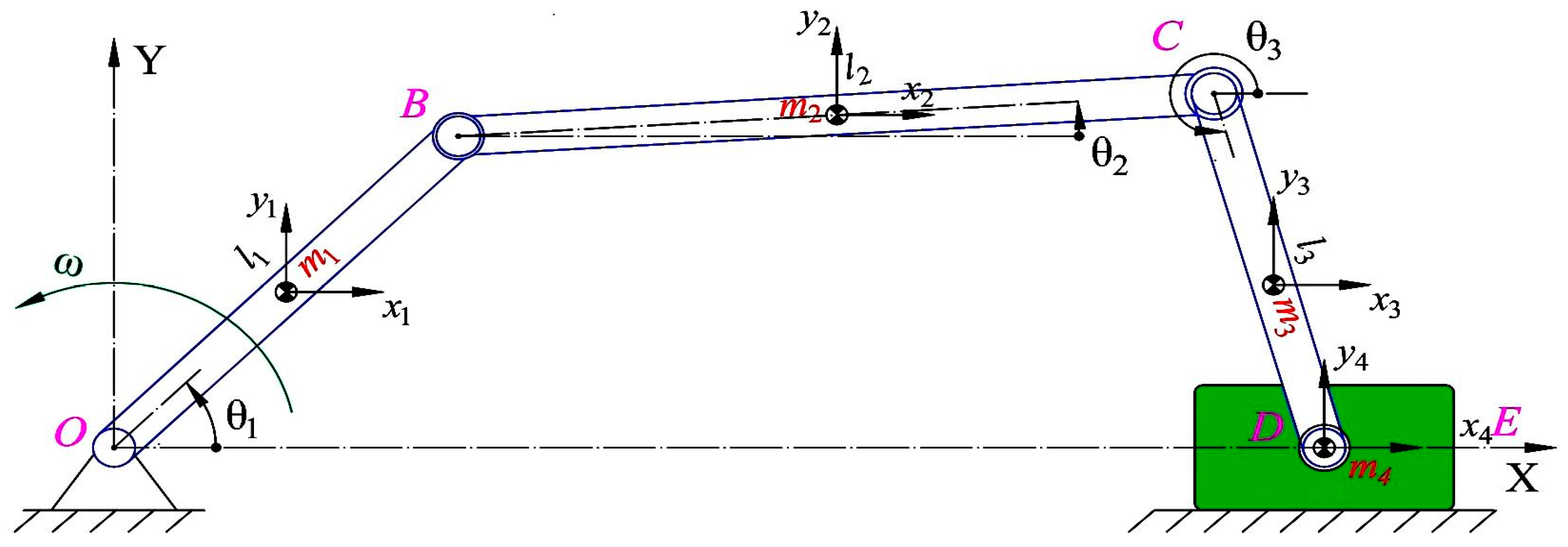
The schematic diagram of the planar closed-chain under-actuated mechanism is shown in Figure 5. In Figure 5, four rotating joints and one translational joint are expressed as O, B, C, D, and E. At the same time, O is both the origin of coordinates and the driving joint. The lengths of the linkages OB, BC, and CD are labeled as l₁, l₂, and l₃, while their respective masses are represented by m₁, m₂, and m₃. The mass of the slider E is represented by m₄.

3.1. Numerical Equations

The device in Figure 5 is a special mechanism that has five degrees of freedom. In this paper, the Lagrange equation of the first kind is used to build the dynamic equations. Therefore, the generalized coordinates, $q_j$, and constraint equations, $\Phi$, are chosen as follows:

$$q_j=\{{\theta }_1,{\theta }_2,{\theta }_3,x_4\}$$

(8)

$$\Phi =\left[\begin{array}{c}{l}_1\sin {\theta }_1+l_2\sin {\theta }_2+l_3\sin {\theta }_3=0\\ l_1\cos {\theta }_1+l_2\cos {\theta }_2+l_3\cos {\theta }_3=x_4\end{array}\right]\iff \left[\begin{array}{c}{\lambda }_1\\ {\lambda }_2\end{array}\right]$$

(9)

The equation of motion is given as follows [31]:

$${\displaystyle \frac{d}{dt}}({\displaystyle \frac{\mathsf{\partial }T}{\mathsf{\partial }{\dot{q}}_j}})-{\displaystyle \frac{\mathsf{\partial }T}{\mathsf{\partial }{q}_j}}=Q_j+{\displaystyle \sum _{i=1}^s{\lambda }_i\frac{\mathsf{\partial }{f}_i}{\mathsf{\partial }{q}_j}}$$

(10)

where T is the system’s kinetic energy, $Q_j$ is the generalized force, ${\lambda }_i$ is the Lagrange multiplier, and $f_i$ is the system constraint equation.

The kinetic energy of the mechanism is given as follows:

$$T={\displaystyle \frac{1}{2}}{m}_1({{\dot{x}}_1}^2+{{\dot{y}}_1}^2)+{\displaystyle \frac{1}{2}}{m}_2({{\dot{x}}_2}^2+{{\dot{y}}_2}^2)+{\displaystyle \frac{1}{2}}{m}_3({{\dot{x}}_3}^2+{{\dot{y}}_3}^2)+{\displaystyle \frac{1}{2}}{m}_4{{\dot{x}}_4}^2+{\displaystyle \frac{1}{2}}(J_1{\dot{\theta }}_1^2+J_2{\dot{\theta }}_2^2+J_3{\dot{\theta }}_3^2)$$

(11)

in which

$$\begin{array}{l}{\dot{x}}_1=-l_1\sin {\theta }_1{\dot{\theta }}_1/2\\ {\dot{y}}_1=l_1\cos {\theta }_1{\dot{\theta }}_1/2\\ {\dot{x}}_2=-l_1\sin {\theta }_1{\dot{\theta }}_1-l_2\sin {\theta }_2{\dot{\theta }}_2/2\\ {\dot{y}}_2=l_1\cos {\theta }_1{\dot{\theta }}_1+l_2\cos {\theta }_2{\dot{\theta }}_2/2\\ {\dot{x}}_3=-l_1\sin {\theta }_1{\dot{\theta }}_1-l_2\sin {\theta }_2{\dot{\theta }}_2-l_3\sin {\theta }_3{\dot{\theta }}_3/2\\ {\dot{y}}_2=l_1\cos {\theta }_1{\dot{\theta }}_1+l_2\cos {\theta }_2{\dot{\theta }}_2+l_3\cos {\theta }_3{\dot{\theta }}_3/2\end{array}$$

Then, Equation (11) can be written as follows:

$$\begin{array}{l}T={\dot{\theta }}_1^2({\displaystyle \frac{1}{8}}{m}_1{l}_1^2+{\displaystyle \frac{1}{2}}{J}_1+{\displaystyle \frac{1}{2}}{m}_2{l}_1^2+{\displaystyle \frac{1}{2}}{m}_3{l}_1^2)+{\dot{\theta }}_2^2({\displaystyle \frac{1}{8}}{m}_2{l}_2^2+{\displaystyle \frac{1}{2}}{J}_2+{\displaystyle \frac{1}{2}}{m}_3{l}_2^2)+{\dot{\theta }}_3^2({\displaystyle \frac{1}{8}}{m}_3{l}_3^2+{\displaystyle \frac{1}{2}}{J}_3)+{\displaystyle \frac{1}{2}}{m}_4{\dot{x}}_4^2\\ \hspace{1em}\hspace{1em}+({\displaystyle \frac{1}{2}}{m}_2+m_3)l_1{l}_2{\dot{\theta }}_1{\dot{\theta }}_2(\sin {\theta }_1\sin {\theta }_2+\cos {\theta }_1\cos {\theta }_2)+{\displaystyle \frac{1}{2}}{m}_3{l}_1{l}_3{\dot{\theta }}_1{\dot{\theta }}_3(\sin {\theta }_1\sin {\theta }_3+\cos {\theta }_1\cos {\theta }_3)\\ \hspace{1em}\hspace{1em}+{\displaystyle \frac{1}{2}}{m}_3{l}_2{l}_3{\dot{\theta }}_2{\dot{\theta }}_3(\sin {\theta }_2\sin {\theta }_3+\cos {\theta }_2\cos {\theta }_3)\end{array}$$

(12)

Based on Equations (9), (10), and (12), the acceleration equations for the generalized coordinates ${\theta }_2$, ${\theta }_3$, and $x_4$ are derived as follows:

$$\begin{array}{l}{\theta }_2:{\ddot{\theta }}_2({\displaystyle \frac{1}{4}}{m}_2{l}_2^2+J_2+m_3{l}_2^2)+{\displaystyle \frac{1}{2}}{m}_3{l}_2{l}_3{\ddot{\theta }}_3(\sin {\theta }_2\sin {\theta }_3+\cos {\theta }_2\cos {\theta }_3)\\ \hspace{1em}+({\displaystyle \frac{1}{2}}{m}_2+m_3)l_1{l}_2{\dot{\theta }}_1^2(\cos {\theta }_1\sin {\theta }_2-\sin {\theta }_1\cos {\theta }_2)\\ \hspace{1em}+{\displaystyle \frac{1}{2}}{m}_3{l}_2{l}_3{\dot{\theta }}_3^2(\sin {\theta }_2\cos {\theta }_3-\cos {\theta }_2\sin {\theta }_3)=M{r}_2+{\lambda }_1{l}_2\cos {\theta }_2-{\lambda }_2{l}_2\sin {\theta }_2\end{array}$$

(13)

$$\begin{array}{l}{\theta }_3:{\ddot{\theta }}_2{\displaystyle \frac{1}{2}}{m}_3{l}_2{l}_3(\sin {\theta }_2\sin {\theta }_3+\cos {\theta }_2\cos {\theta }_3)+{\ddot{\theta }}_3({\displaystyle \frac{1}{4}}{m}_3{l}_3^2+J_3)\\ \hspace{1em}+{\displaystyle \frac{1}{2}}{m}_3{l}_1{l}_3{\dot{\theta }}_1^2(\cos {\theta }_1\sin {\theta }_3-\sin {\theta }_1\cos {\theta }_3)\\ \hspace{1em}+{\displaystyle \frac{1}{2}}{m}_3{l}_2{l}_3{\dot{\theta }}_2^2(\cos {\theta }_2\sin {\theta }_3-\sin {\theta }_2\cos {\theta }_3)=M{r}_3+{\lambda }_1{l}_3\cos {\theta }_3-{\lambda }_2{l}_3\sin {\theta }_3\end{array}$$

(14)

$$x_4: m_4{\ddot{x}}_4=F_f-{\lambda }_2$$

(15)

where ${Mr}_2$ and ${Mr}_3$ represent the external torque applied to joint ${\theta }_2$ and ${\theta }_3$, respectively, and $F_f$ represents the frictional resistance of slider E.

Since ${\theta }_1$ represents the driving speed, its speed is a fixed value, and its acceleration is zero.

Based on the Baumgarte approach, Equation (9) can be written as follows:

$$\begin{array}{l}{l}_2\cos {\theta }_2{\ddot{\theta }}_2+l_3\cos {\theta }_3{\ddot{\theta }}_3=l_1\sin {\theta }_1{\dot{\theta }}_1^2+l_2\sin {\theta }_2{\dot{\theta }}_2^2+l_3\sin {\theta }_3{\dot{\theta }}_3^2\\ \hspace{1em}\hspace{1em}\hspace{1em}\hspace{1em}\hspace{1em}\hspace{1em}\hspace{1em}\hspace{1em}-\epsilon (l_1\cos {\theta }_1{\dot{\theta }}_1+l_2\cos {\theta }_2{\dot{\theta }}_2+l_3\cos {\theta }_3{\dot{\theta }}_3)-\beta (l_1\sin {\theta }_1+l_2\sin {\theta }_2+l_3\sin {\theta }_3)\end{array}$$

(16)

$$\begin{array}{l}{l}_2\cos {\theta }_2{\ddot{\theta }}_2+l_3\cos {\theta }_3{\ddot{\theta }}_3=l_1\sin {\theta }_1{\dot{\theta }}_1^2+l_2\sin {\theta }_2{\dot{\theta }}_2^2+l_3\sin {\theta }_3{\dot{\theta }}_3^2\\ \hspace{1em}\hspace{1em}\hspace{1em}\hspace{1em}\hspace{1em}\hspace{1em}\hspace{1em}\hspace{1em}-\epsilon (l_1\cos {\theta }_1{\dot{\theta }}_1+l_2\cos {\theta }_2{\dot{\theta }}_2+l_3\cos {\theta }_3{\dot{\theta }}_3)-\beta (l_1\sin {\theta }_1+l_2\sin {\theta }_2+l_3\sin {\theta }_3)\end{array}$$

(17)

Here, $\mathsf{\epsilon }$ and $\mathsf{\beta }$ are important parameters in the Baumgarte approach, whose values are $\sqrt{2}/h$ and $1/h$, respectively, while h is the simulation step size, whose value is 1 × 10⁻⁵.

Based on Equations (13)–(17), the acceleration of ${\theta }_2$, ${\theta }_3$ and $x_4$ are derived as follows:

$${\ddot{\theta }}_3=(H_{11}{l}_3\cos {\theta }_3-l_2\cos {\theta }_2{H}_{13})/(l_3\cos {\theta }_3{H}_{10}-l_2\cos {\theta }_2{H}_{12})$$

(18)

$${\lambda }_1=(H_{10}{\ddot{\theta }}_3-H_{11})/(l_2^2{\cos }^2{\theta }_2)$$

(19)

$${\ddot{\theta }}_2=(H_7-l_3\cos {\theta }_3{\ddot{\theta }}_3)/(l_2\cos {\theta }_2)$$

(20)

$${\lambda }_2={\ddot{\theta }}_3{H}_9+(F_f-m_4\ast H_8)$$

(21)

$${\ddot{x}}_4=(F_f-{\lambda }_2)/m_4$$

(22)

in which

$$\begin{array}{l}{H}_1=m_2{l}_2^2/4+J_2+m_3{l}_2^2\\ H_2=m_3{l}_2{l}_3(\sin {\theta }_2\sin {\theta }_3+\cos {\theta }_2\cos {\theta }_3)/2\\ H_3=M{r}_2-(m_2/2+m_3)l_1{l}_2{\dot{\theta }}_1^2(\cos {\theta }_1\sin {\theta }_2-\sin {\theta }_1\cos {\theta }_2)\\ \hspace{1em}\hspace{1em}-m_3{l}_2{l}_3{\dot{\theta }}_3^2(\sin {\theta }_2\cos {\theta }_3-\cos {\theta }_2\sin {\theta }_3)/2\\ H_4=m_3{l}_2{l}_3(\sin {\theta }_2\sin {\theta }_3+\cos {\theta }_2\cos {\theta }_3)/2\\ H_5=m_3{l}_3^2/4+J_3\\ H_6=M{r}_3-0.5m_3{l}_1{l}_3{\dot{\theta }}_1^2(\cos {\theta }_1\sin {\theta }_3-\sin {\theta }_1\cos {\theta }_3)\\ \hspace{1em}\hspace{1em}-0.5m_3{l}_2{l}_3{\dot{\theta }}_2^2(\cos {\theta }_2\sin {\theta }_3-\sin {\theta }_2\cos {\theta }_3)\\ H_7=l_1\sin {\theta }_1{\dot{\theta }}_1^2+l_2\sin {\theta }_2{\dot{\theta }}_2^2+l_3\sin {\theta }_3{\dot{\theta }}_3^2\\ \hspace{1em}\hspace{1em}-\epsilon (l_1\cos {\theta }_1{\dot{\theta }}_1+l_2\cos {\theta }_2{\dot{\theta }}_2+l_3\cos {\theta }_3{\dot{\theta }}_3)-\beta (l_1\sin {\theta }_1+l_2\sin {\theta }_2+l_3\sin {\theta }_3)\\ H_8=-l_1\cos {\theta }_1{\dot{\theta }}_1^2-l_2\cos {\theta }_2{\dot{\theta }}_2^2-l_3\cos {\theta }_3{\dot{\theta }}_3^2\\ \hspace{1em}\hspace{1em}-\epsilon (l_1\sin {\theta }_1{\dot{\theta }}_1+l_2\sin {\theta }_2{\dot{\theta }}_2+l_3\sin {\theta }_3{\dot{\theta }}_3+{\dot{x}}_4)+\beta (l_1\cos {\theta }_1+l_2\cos {\theta }_2+l_3\cos {\theta }_3-x_4)\\ H_9=(l_2\cos {\theta }_2{m}_4{l}_3\sin {\theta }_3-m_4{l}_2\sin {\theta }_2{l}_3\cos {\theta }_3)/(l_2\cos {\theta }_2)\\ H_{10}=l_2\cos {\theta }_2{H}_2-H_1{l}_3\cos {\theta }_3+l_2^2\cos {\theta }_2\sin {\theta }_2{H}_9\\ H_{11}=(m_4{H}_8-F_f)l_2^2\cos {\theta }_2\sin {\theta }_2+l_2\cos {\theta }_2{H}_3-H_1{H}_7\\ H_{12}=l_2\cos {\theta }_2{H}_5-H_4{l}_3\cos {\theta }_3+H_9{l}_2\cos {\theta }_2{l}_3\sin {\theta }_3\\ H_{13}=(m_4{H}_8-F_f)l_2\cos {\theta }_2{l}_3\sin {\theta }_3+l_2\cos {\theta }_2{H}_6-H_4{H}_7\end{array}$$

3.2. Numerical Solution and Analysis

In this section, based on Equations (18)–(22), described in Section 3.1, the Runge–Kutta method is used to solve the dynamic behavior of the planar closed-chain under-actuated mechanism. The parameters of the mechanism are listed in

Table 1. The parameters of the under-actuated mechanism.

Link	Length	Mass	Moment of Inertia
l1	0.14 m	0.131 kg	0.00004684 kg/m2
l2	0.32 m	0.3 kg	0.00010706 kg/m2
l3	0.16 m	0.15 kg	0.00005353 kg/m2
m3	unused	0.698 kg	unused

.

Because the under-actuated mechanism is sensitive to the initial value, it is important to ensure that the initial conditions of each dynamic calculation and experiment are the same. The initial angles of ${\theta }_1$, ${\theta }_2$, and ${\theta }_3$ are all zero, and the slider E is on the right. The schematic diagram of the initial state of the system is shown in Figure 6.

The initial value is important for the Runge–Kutta method. In Figure 6, ${\theta }_1$= 0, ${\theta }_2$= 0, ${\theta }_3$= 0, and $x_4$= l₁ + l₂ + l₃; meanwhile, ${\dot{\theta }}_1=\mathsf{\omega }$, ${\dot{\theta }}_2$ = 0, ${\dot{\theta }}_3=-l_1\mathrm{c}\mathrm{o}\mathrm{s}{\theta }_1\mathsf{\omega }/\left(l_3\mathrm{c}\mathrm{o}\mathrm{s}{\theta }_3\right)$, and ${\dot{x}}_4=0$. By changing the driving speed, $\mathsf{\omega }$, and the length of l₃, the chaos intensity curves of the system under different parameters are obtained, as shown in Figure 7.

Figure 7 shows that with the change in driving speed and the length of l₃, the chaos intensity of the system undergoes significant change, especially when the driving speed is 1200 r/min, at which point the chaos intensity of the system is obviously suppressed and enhanced. When $\mathsf{\omega }=1$200 r/min, l₃ = 0.06 m, and the system exhibits chaos suppression, and when $\mathsf{\omega }=1$200 r/min, l₃ = 0.151 m, and the system exhibits chaos enhancement. The results are shown in Figure 8a and Figure 8b, respectively.

In order to ensure the proportional coordination of the phase diagram in Figure 8, the unit of the displacement of the slider E(x₄) is decimeters. In Figure 8a, the distribution of data points is relatively concentrated, indicating that the chaos intensity of the system is suppressed. In Figure 8b, the distribution of data points is relatively divergent, indicating that the chaos intensity of the system is enhanced.

4. Optimization Example

According to the analysis in Section 3, in the closed-chain under-actuated five-bar mechanism, the length of the linkage and the size of the driving speed will cause a change in the chaos intensity of the system. In order to suppress and enhance the chaos intensity of the system, based on PSO, the maximum and minimum of the uniformity value are taken as the optimization objectives, and the linkage length and driving speed of the mechanism are taken as the optimal calculation parameters. This optimization mainly considers changing the force of the end slider by optimizing the lengths of the linkages, thus changing its mass and center of gravity position [28]. The optimization algorithm is shown in

Table 2. Particle swarm optimization parameters.

Optimization Parameters	Mathematical Expression
Objective	min(L) and max(L)
Dynamic parameters	$40 \mathrm{r}/\mathrm{m}\mathrm{i}\mathrm{n}\le \mathsf{\omega }\le 400 \mathrm{r}/\mathrm{m}\mathrm{i}\mathrm{n}$, $l_1$ = 0.14 m, $0.01 \mathrm{m} \le l_3 \le 0.16 \mathrm{m}$, $l_2=\left(0.48-l_3\right) \mathrm{m}$
Speed update	${\mathrm{V}}_{\mathrm{i}\mathrm{d}}=\mathsf{\varpi }{\mathrm{V}}_{\mathrm{i}\mathrm{d}}+{\mathrm{C}}_1\mathrm{r}\mathrm{a}\mathrm{n}\mathrm{d}\mathrm{o}\mathrm{n}\left(\mathrm{0,1}\right)\left({\mathrm{P}}_{\mathrm{i}\mathrm{d}}-{\mathrm{X}}_{\mathrm{i}\mathrm{d}}\right)+{\mathrm{C}}_2\mathrm{r}\mathrm{a}\mathrm{n}\mathrm{d}\mathrm{o}\mathrm{m}\left(\mathrm{0,1}\right)\left({\mathrm{P}}_{\mathrm{g}\mathrm{d}}-{\mathrm{X}}_{\mathrm{i}\mathrm{d}}\right)$
Position update	${\mathrm{X}}_{\mathrm{i}\mathrm{d}}={\mathrm{X}}_{\mathrm{i}\mathrm{d}}+{\mathrm{V}}_{\mathrm{i}\mathrm{d}}$

.

In Table 2, due to the limitation of our experimental equipment, $40 \mathrm{r}/\mathrm{m}\mathrm{i}\mathrm{n}\le \mathsf{\omega }\le 400 \mathrm{r}/\mathrm{m}\mathrm{i}\mathrm{n}$; $\mathsf{\varpi }$ is the inertia factor, ${\mathrm{C}}_1$ and ${\mathrm{C}}_2$ are acceleration constants; generally, ${\mathrm{C}}_1$ = ${\mathrm{C}}_2\in$ [0, 4]; random (0, 1) indicates a random number in the range of 0 to 1; ${\mathrm{P}}_{\mathrm{i}\mathrm{d}}$ represents the individual extreme value of the ith variable; and ${\mathrm{P}}_{\mathrm{g}\mathrm{d}}$ represents the global optimal solution.

According to Table 1, the suppression and enhancement of chaotic phenomena in the system will be realized. In order to test the reliability of the dynamic simulation, based on the schematic diagram shown in Figure 6 and the parameters in Table 1, the experimental platform shown in Figure 9 was established.

In the system shown in Figure 9, the displacement data collected by the grating ruler are transmitted to LabVIEW through STM32. STM32 is a series of 32-bit microcontrollers (MCUs) produced by STMicroelectronics. This paper mainly uses the chip to collect data; then, the collected data are used to calculate the system speed based on time.

4.1. Chaos Suppression

When the chaos intensity value of the system is small, the force on the end slider E of the mechanism is uniform. As shown in Figure 10, the phenomenon is that the trajectory of the phase diagram composed of the displacement and velocity is smooth, and the data points are concentrated. In order to achieve the above purpose, L is taken as the optimization objective, the initial population number is 10, and the optimization algebra is 10 generations. The optimization result is that when the driving speed is 292.325 r/min, $l_3$= 0.0592 m and the chaos intensity of the system is suppressed. The optimization phase diagram and optimal fitness evolution process are shown in Figure 10.

In Figure 10a, the data points of the phase diagram are concentrated, and the motion curve is smooth, which indicates that the force of the end slider is uniform during movement. Figure 10b shows that PSO has been looking for system parameters with low values of L. In Figure 10, the numerical simulation and experimental results show that the chaos intensity of the system is suppressed under this parameter.

4.2. Chaos Enhancement

When the chaos intensity value of the system is high, the force variation of the end slider E of the mechanism is strong. As shown in Figure 11, the mechanism is that the phase diagram trajectory composed of the displacement and velocity has a large and irregular variation interval, and the data points are relatively divergent. In order to achieve the above purpose, L is taken as the optimization objective, the initial population number is 10, and the optimization algebra is 10 generations. The optimization result is that when the drive speed is 391.255 r/min, $l_3$= 0.0592 m, which indicates that the chaos intensity of the system is enhanced. The optimization phase diagram and the evolution process of optimal fitness are shown in Figure 11.

In Figure 11a, the data points of the phase diagram diverge, and the motion curves are irregular, which indicates that the force of the end slider changes significantly during movement. Figure 11b shows that PSO has been looking for system parameters with higher values of L. In Figure 11, the numerical simulation and experimental results show that the chaotic motion intensity of the system is improved under these parameters. Figure 11b shows that the optimization of the system has reached stability.

It can be seen from Figure 10 and Figure 11 that uniformity and PSO are used to successfully suppress and enhance the chaos intensity of a planar closed-chain under-actuated mechanism, and the experimental results verify the accuracy of dynamic modeling and the reliability of uniformity in determining the chaos intensity of the system.

5. Conclusions

In this paper, uniformity is used to determine the chaos intensity of nonlinear mechanical systems for the first time. With the help of a closed-chain under-actuated five-bar mechanism, the chaos intensity is suppressed and strengthened under different parameters. Uniformity achieves the suppression and enhancement of system’s chaos intensity by monitoring the distribution of data points in the phase diagram composed of the displacement and velocity caused by different driving speeds and connecting rod lengths. At the end of the article, the PSO is successfully applied to enhance and suppress the chaos intensity of the system.

In the dynamic analysis, the first Lagrange equation is used to establish the dynamic equation of the system, and the Runge–Kutta method is the solution of the system. The experimental platform verifies the optimization results of the PSO and also proves the accuracy of the dynamic modeling method and the high efficiency of the uniformity used to determine the chaotic intensity of the system.

This paper successfully applies the uniformity theory to the judgment of chaos intensity of nonlinear mechanical systems for the first time, which provides a new way for other scholars to analyze nonlinear systems. In the future, how to apply the chaos intensity determination method to different systems, reduce the impact of the difference in the amount of system data points on the results, and improve the accuracy of this method will have high research value.