An Advanced Approach for Predicting Workpiece Surface Roughness Using Finite Element Method and Image Processing Techniques

Abstract

Workpiece surface quality is a critical metric for assessing machining quality. However, due to the complex coupling characteristics of cutting factors, accurately predicting surface roughness remains challenging. Typically, roughness is measured post-machining using specialized instruments, which delays feedback and hampers timely problem detection, ultimately resulting in cutting resource wastage. To address this issue, this paper introduces a predictive model for workpiece surface roughness based on the finite element (FE) method and advanced image processing techniques. Initially, an orthogonal turning experiment was designed, and an FE cutting model was constructed to assess the distribution of cutting forces and temperatures under varying cutting parameters. Image processing methods (including mesh calibration, edge extraction, and contour fitting) were then applied to extract surface characteristics from the FE simulation outputs, yielding preliminary estimates of surface roughness. By employing range and regression analyses methods, this study quantitatively evaluates the interdependencies among cutting parameters, forces, temperatures, and roughness, subsequently formulating a multivariate regression model to predict surface roughness. Finally, a turning experiment under actual working conditions was conducted, confirming the model’s capacity to predict the $R_a$ trend with an accuracy of 85.07%. Thus, the proposed model provides a precise predictive tool for surface roughness, offering valuable guidance for optimizing machining parameters and supporting proactive control in the turning process, ultimately enhancing machining efficiency and quality.

1. Introduction

Turning is a fundamental metal-cutting process renowned for its precision and efficient material removal capabilities. A comprehensive understanding of the complex interrelationships between cutting parameters, cutting forces, and heat generation during the turning process—as well as their impact on surface texture and quality—is critical for optimizing machining parameters, predicting process outcomes, and enhancing surface finishes. Bian et al. [1] investigated the influence of the main process parameters of UV picosecond laser cutting on the cutting quality of 22MnB5 plates. And they found that laser parameters are the important influences on the roughness of the cutting surface and the subgrain layer. Similarly, Cui et al. [2] used SEM measurements to observe the impact of random run-out on surface roughness in milling, revealing that chip residue significantly compromises surface integrity and increases roughness. However, traditional approaches to selecting optimal cutting parameters often rely on empirical methods and trial-and-error experimentation, which can limit the optimization scope and impede optimal process performance. This approach also leads to material waste and unnecessary labor costs [3].

Advancements in computer technology and simulation tools have made the finite element method (FEM) a valuable asset in turning process modeling under various cutting conditions [4]. Improvements in material constitutive models and meshing techniques have expanded FEM’s application in machining research [5,6], including studies of chip formation, cutting forces, temperature, tool wear, and microstructural evolution [7]. For example, Ye et al. [8] used FEM to characterize serrated chip formation, while Liu et al. [9] applied the Abaqus to investigate tool morphology impacts on thin-walled workpieces. Similarly, Muhammad et al. [10] developed a 3D thermomechanical coupled finite element (FE) model for conventional ultrasonically assisted turning, and other studies have investigated parameter–tool wear interactions and temperature distribution under varying cooling conditions [11]. Collectively, these studies demonstrate FEM’s robust potential for simulating cutting processes [12].

Surface quality is critical in determining the mechanical properties of machined parts, such as fatigue strength, tribological performance, and corrosion resistance [13]. Consequently, considerable research has focused on monitoring surface quality in machining processes. However, conventional offline methods, such as digital microscopy and profilometry, present limitations: they are prone to interference, demand extensive experimental setups, and involve complex procedures [14]. These limitations highlight the need for more efficient, accurate methods to assess surface quality. Jia et al. [15] integrated the multi-objective optimization model for rough and finish cutting parameters in plane milling. Wang et al. [16] investigated the effects of wire saw processing parameters and sawing direction on the surface roughness and warpage of monocrystalline silicon, developing an anisotropic sawing model to predict processing forces, surface roughness, and warpage. Li et al. [17] optimized Magnetic Field-Assisted Blast Erosion Arc Machining (M-BEAM) using the Nelder–Mead algorithm to identify optimal parameter combinations, which reduced Surface Roughness (Sa) by 25.96% and 60.61% in roughing and finishing, respectively. Pei et al. [18] designed a multi-task dual-domain adaptive deep transfer learning to train the cutting forces and milling parameters and predicted the geometric errors of machining holes for milling thin-walled parts. However, this model only works effectively when data domains have high similarity.

Finite element analysis offers a promising solution by enabling surface roughness prediction while reducing the associated economic costs [19,20]. For instance, Yang et al. [21] developed a 3D FE model for diamond turning to assess surface roughness, while others have examined the relationship between cutting parameters and surface quality using FEM [22,23]. Pan et al. [14] used a second-order polynomial model to describe the surface roughness but noted the necessity of accounting for factors such as tool wear [24], heat, material properties, and chip thickness. While FEM offers significant advantages, roughness prediction based on FEM typically requires model construction, which increases computational complexity and processing time [25]. Moreover, integrating FEM with image processing for surface roughness assessment remains relatively unexplored.

This study addresses these gaps by combining image processing techniques with a finite element model generated in Abaqus (2023) to extract surface features and calculate surface roughness using MATLAB (R2023b). The influence of cutting parameters on workpiece surface quality, force, and temperature was analyzed using single-factor and range analysis methods. A multiple linear regression equation was then established to quantify the relationship between cutting depth, cutting speed, ambient temperature, and workpiece temperature on surface roughness. The model’s reliability was validated through the R-squared (R²) index. Finally, turning experiments confirmed that the proposed method can effectively predict workpiece surface roughness under given cutting parameters.

2. Finite Element Modelling of Turning Process

2.1. Material Constitutive Modelling for Cutting

During the cutting process, the surface layer of the workpiece experiences elastic–plastic deformation under conditions of high temperature and high strain. The strain, strain rate, and temperature within the cut layer exhibit non-uniform distributions, characterized by significant gradients. The Johnson–Cook model has proven to be effective in describing the thermal viscoelastic deformation behavior of materials under high-strain-rate conditions [26]. The Johnson–Cook model is expressed in Equation (1):

$$\sigma =[A+B{\epsilon }^N]\left[1+C\mathit{ln}\left({\displaystyle \frac{\stackrel{•}{\epsilon }}{{\stackrel{•}{\epsilon }}_0}}\right)\right]\left[1-{\left({\displaystyle \frac{T-T_0}{T_m-T_0}}\right)}^m\right],$$

(1)

where $\sigma ,{\epsilon }^N,\stackrel{•}{\epsilon },$ and ${\stackrel{•}{\epsilon }}_0$ are the equivalent stress, equivalent strain, equivalent strain rate, and reference strain rate, respectively. $A, B, \alpha ,C$, and $\beta$ are material coefficients, where $A$ is the yield stress under uniaxial tension, and $B$ and $\alpha$ are obtained through fitting stress–strain data. $C$ is the strain-rate sensitivity parameter, and $\beta$ is the temperature softening parameter. $T_0$ and $T_m$ denote the initial temperature and melting point temperature, respectively. In this study, Q235B was employed as the workpiece material, and the parameters in Equation (1) are listed in

Table 1. Constitutive model parameters of Q235B [29].

Yield Stress $\mathbf{A} (\mathbf{M}\mathbf{P}\mathbf{a}$)	Stress–Strain Data Fitting Parameters $\mathbf{B} (\mathbf{M}\mathbf{P}\mathbf{a}$)	Strain Sensitivity Parameters C	Stress–Strain Data Fitting $\mathbf{Parameters} \mathit{\alpha }$	Temperature Softening Parameters $\mathit{\beta }$	Material Melting Point Temperature ${\begin{array}{c} \\ \mathit{T}\end{array}}_{\mathit{m} }(\mathit{℃})$	Initial Temperature ${\mathit{T}}_{0 }(°\mathbf{C})$
244.8	899.7	0.014	0.94	0.757	1521.85	25

. The standard for Q235B refers to [27] GB/T 700-2006, and its chemical composition parameters are presented in

Table 2. The chemical composition of Q235B (%).

C	Si	Mn	P	S
0.20	0.35	1.4	0.045	0.045

. The chemical composition and material properties of Q235B are comparable to those of S235JR specified in EN 10025-2:2019 [28].

The equation for failure strain in this model is given by Equation (2):

$$\omega ={\displaystyle \frac{{\epsilon }^{-pl}+\sum \mathsf{\Delta }{\epsilon }^{-pl}}{{\epsilon }_f^{-pl}}},$$

(2)

where $\omega$ is the failure parameter, ${\epsilon }^{-pl}$ is the initial value of equivalent plastic strain, $\Delta {\epsilon }^{-pl}$ is the increment of equivalent plastic strain, and ${\epsilon }_f^{-pl}$ is the failure strain. The mechanical properties of Q235B are listed in

Table 3. Mechanical properties of Q235B.

$\mathbf{Density} (\mathbf{k}\mathbf{g}/{\mathbf{m}}^3$)	$\mathbf{Conductivity} (\mathbf{m}\mathbf{W}/(\mathbf{m}\mathbf{m}·\mathbf{K})$)	$\mathbf{Young}\text{’}\mathbf{s} \mathbf{Modulus} (\mathbf{M}\mathbf{P}\mathbf{a}$)
7800	43	212,000

.

The cutting tool used was the NX2525 model manufactured by Mitsubishi Corporation, with a specific designation of NGG160402R-F. The mechanical characteristics of the specimens are listed in

Table 4. Mechanical properties of cutting tool.

$\mathbf{Rockwell} \mathbf{Hardness} (\mathbf{H}\mathbf{R}\mathbf{A}$)	Conductivity $(\mathbf{W}/\mathbf{m}.\mathbf{k}$)	Expansion $({10}^{-6}/\mathbf{K}$)	$\mathbf{Bending} \mathbf{Strength} (\mathbf{G}\mathbf{P}\mathbf{a}$)	$\mathbf{Rockwell} \mathbf{Hardness} (\mathbf{H}\mathbf{R}\mathbf{A}$)
92	33	7.8	2	92

.

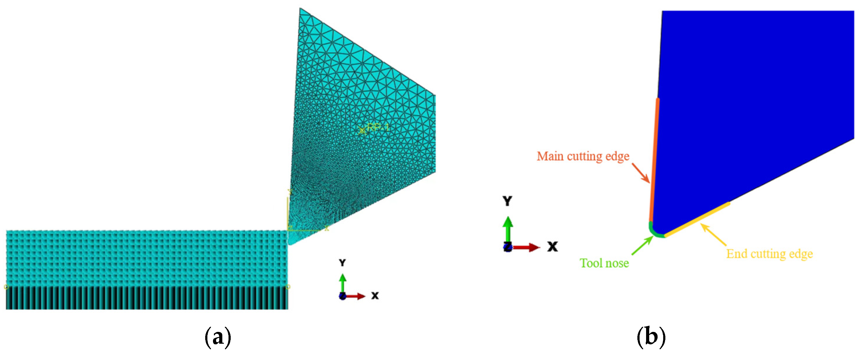
2.2. Turning FE Model Construction

During turning processes, numerous input variables exert influence on output variables. For instance, cutting performance may vary subtly even among tools of the same model, and minor structural differences might exist within workpieces of identical specifications. Additionally, variations in turning machine performance may result in differences in cutting force and surface roughness. Unfortunately, these subtle discrepancies cannot be precisely captured by any single parameter. Moreover, due to computational constraints, it is necessary to simplify the finite element model to optimize efficiency, assuming a more idealized turning model where identical tools, workpieces, machines, and other variables are considered uniform and have negligible impact on the outputs.

Therefore, in the FE model of this turning operation, the workpiece was strategically divided into cutting and non-cutting layers, with a 3 mm cutting layer thickness. This partitioning approach helps balance efficiency without compromising accuracy. As shown in Table 3 and Table 4, the strength of the tool is much higher than that of the workpiece material. The cutting force and temperature variations, as detailed in

Table 5. FES results of cutting force and cutting temperature.

	Factors (H)				Dependent Variable (M)
	${\mathit{A}}_{\mathit{p}}$$(\mathbf{m}\mathbf{m}$)	$\mathbf{V}$ $(\mathbf{m}/\mathbf{m}\mathbf{i}\mathbf{n}$)	${\mathit{T}}_{\mathit{e}}$$(\mathbf{°}\mathbf{C})$	${\mathit{T}}_{\mathbf{0} }(°\mathbf{C})$	$\mathit{F}$ $(\mathbf{N}$P)	${\mathit{T}}_{\mathit{c}}$ $(°\mathbf{C})$	${\mathit{T}}_{\mathit{t}\mathit{i}\mathit{p}}$ $(°\mathbf{C})$
1	0.5	23	−5	25	1156.882	100.598	335.875
2	0.5	40	10	150	1102.146	230.063	569.11
3	0.5	57	25	275	1174.938	345.761	767.819
4	0.5	73	40	400	1198.121	564.005	954.454
5	1	23	10	275	1841.327	317.102	494.456
6	1	40	−5	400	1982.513	501.765	661.162
7	1	57	40	25	1983.465	276.969	693.212
8	1	73	25	150	1963.750	310.250	747.441
9	1.5	23	25	400	2696.075	527.120	621.308
10	1.5	40	40	275	2699.128	477.400	553.558
11	1.5	57	−5	150	2785.703	482.18	689.275
12	1.5	73	10	25	2768.397	245.600	690.892
13	2	23	40	150	3401.107	266.800	414.796
14	2	40	25	25	3510.446	250.580	504.199
15	2	57	10	400	3502.793	555.200	858.687
16	2	73	−5	275	3440.002	482.550	905.883

, were prioritized as dependent variables within the cutting region. Considering the transient nature of the cutting process and the relatively small size of the cutting zone, we have conservatively set the workpiece dimensions in the model to a radius of 12 mm and a length of 20 mm.

Regarding mesh generation, structured grids were chosen because they are simple and can produce high-quality meshes [30,31]. Consequently, we adopted structured grids, with the workpiece structured as quadrilateral grids, using the CPE4RT mesh type in Abaqus. The mesh size for the workpiece was set at 0.05 mm, resulting in a total of 32,400 grids. The tool used free triangular meshes of the type CPE3T, controlled by sizes ranging from 0.01 to 0.5 mm. The total number of grids for the tool was 9758, as illustrated in Figure 1a. Considering the relative simplicity of the cutting model, a commonly used penalty friction contact constraint was employed to simplify the computation. Based on the properties of Q235B material, the friction coefficient was set to 0.34 [32]. A thermal coupling model was established between the tool and the workpiece. For efficient computation, the cutting speed determined the finite element analysis steps, which were divided into 100 increments, with an average computation time of 12 h per model. For the cutting tool, the cutting edges and force points involved in the turning process included the leading cutting edge, end cutting edge, tool nose, and crater, as shown in Figure 1b.

3. Methodology Description

The surface quality of a workpiece is influenced by multiple factors, including cutting speed, depth of cut, cutting heat, friction, and vibrations during machining. These factors are often interrelated, resulting in complex nonlinear interactions. To study these effects, orthogonal experimental designs are commonly employed in engineering applications. However, due to the broad range of cutting parameters and the coupling effects among various factors, the process can be time-intensive, leading to low experimental efficiency and significant time requirements in turning operations.

To address these challenges, we developed a finite element (FE) model for the turning process of Q235B. In this study, orthogonal simulation experiments were designed, selecting four primary cutting parameters [33]—cutting depth $A_p$, cutting speed $v$, ambient temperature $T_e$, and initial temperature of the workpiece $T_0$—as factors (H) that have a substantial impact on cutting surface quality. The effects of these four factors on cutting force, temperature, and surface quality were examined [34]. Each factor was set to four different levels; for instance, the values for factor $A_p$ were set to 0.5, 1.0, 1.5, and 2 mm. Each combination of parameters was assigned an experimental test number ranging from 1 to 16, as shown in

Table 6. The arithmetic means deviation of the workpiece surface profile $R_a$.

Test No.	1	2	3	4	5	6	7	8
$R_a$ ($\mathsf{\mu }\mathrm{m}$)	7.698	5.600	4.829	5.865	12.267	11.042	6.118	11.635
Test No.	9	10	11	12	13	14	15	16
$R_a$ ($\mathsf{\mu }\mathrm{m}$)	10.423	10.711	9.442	7.010	8.972	12.682	15.2528	13.428

.

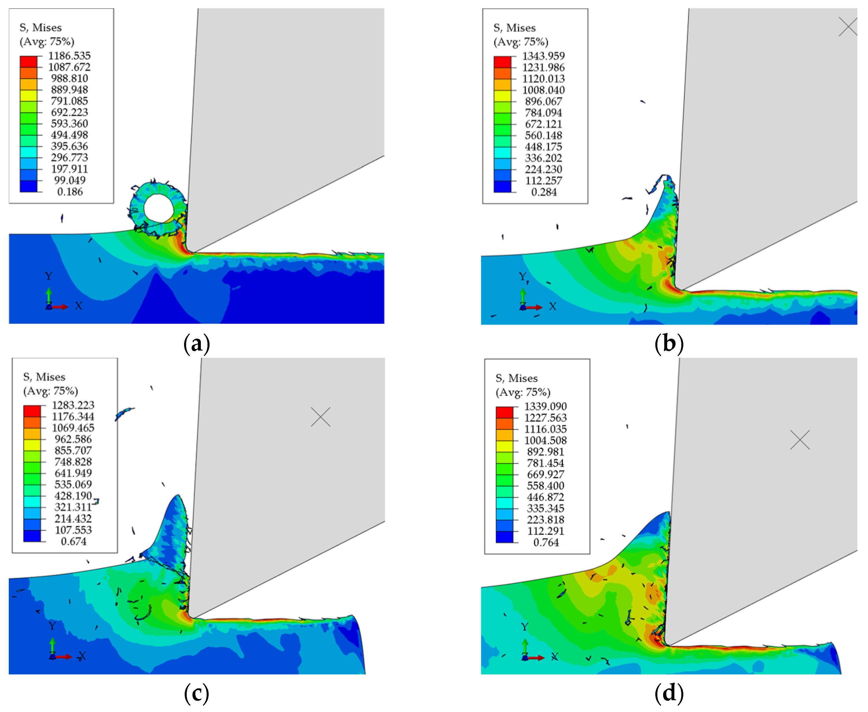
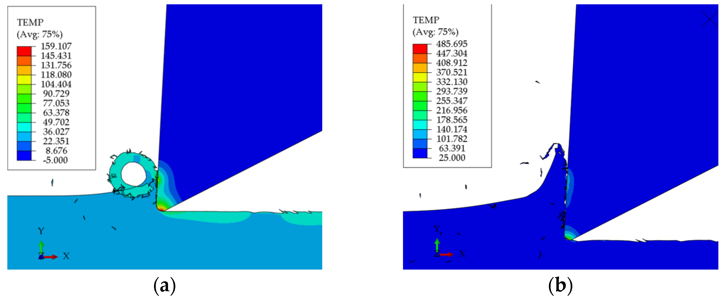
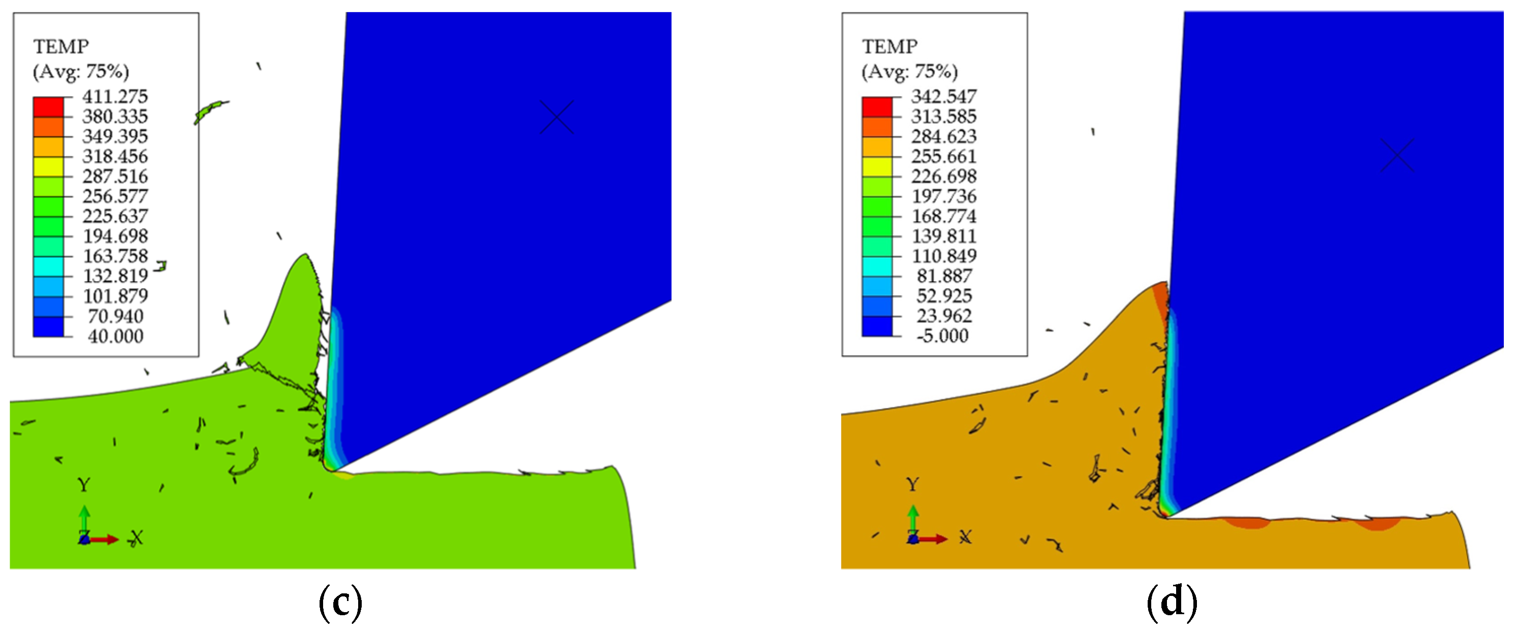
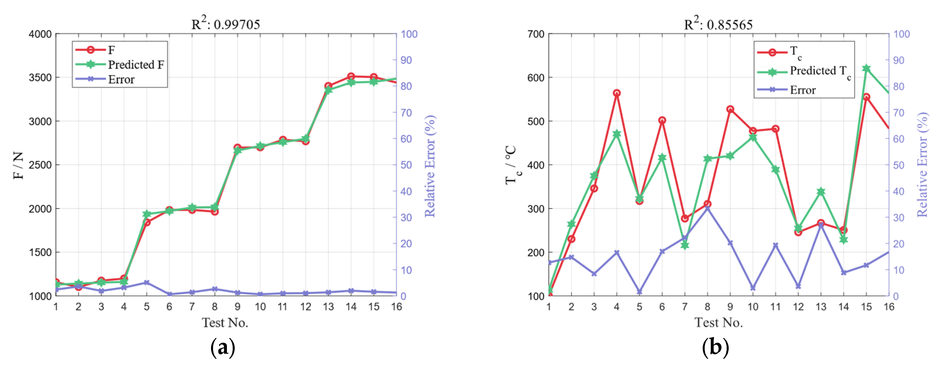
3.1. Cutting Forces and Temperatures Analysis

The cutting speed and depth of the cut regulate the magnitude of the cutting force. These forces cause cutting vibrations, which affect the texture and quality of the workpiece surface [35]. Simultaneously, it has been noted that under constant cutting parameters, variations in cutting temperature can significantly affect the cutting forces, leading to variations in the subsurface damage [36]. Therefore, this study developed an orthogonal simulation experiment encompassing different cutting forces and temperatures. As depicted in Figure 2, the force clouds for test numbers 1, 7, 10, and 16 were generated using FES. The primary cutting force $F$ was determined using Equation (3):

$$F=\sqrt{{F_x}^2+{F_y}^2},$$

(3)

where $F_x$ and $F_y$ are the maximum values of the cutting forces in the X and Y directions, respectively, as extracted from the stable portions of the FES results (shown in Figure 2).

In this simulation, due to the tool settings and installation angle, the cutting edge at the end of the tool (as shown in Figure 1b) did not make contact with the workpiece. Therefore, the analysis focused solely on the temperatures of the main cutting edge ($T_c$) and the tool nose ($T_{tip}$). The maximum temperature values were extracted from the simulation results once a stable turning process was achieved. Figure 3 presents the temperature distributions (cloud diagrams) for Tests 1, 7, 10, and 16.

According to the results of the FES, the cutting force and temperature results obtained for each experimental data set are summarized and listed in Table 5.

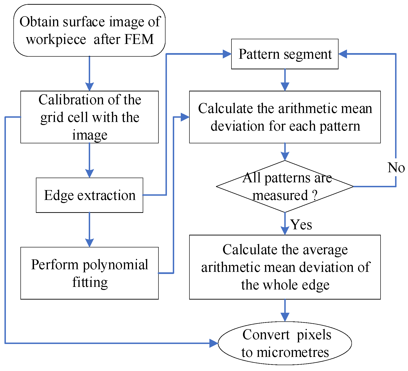
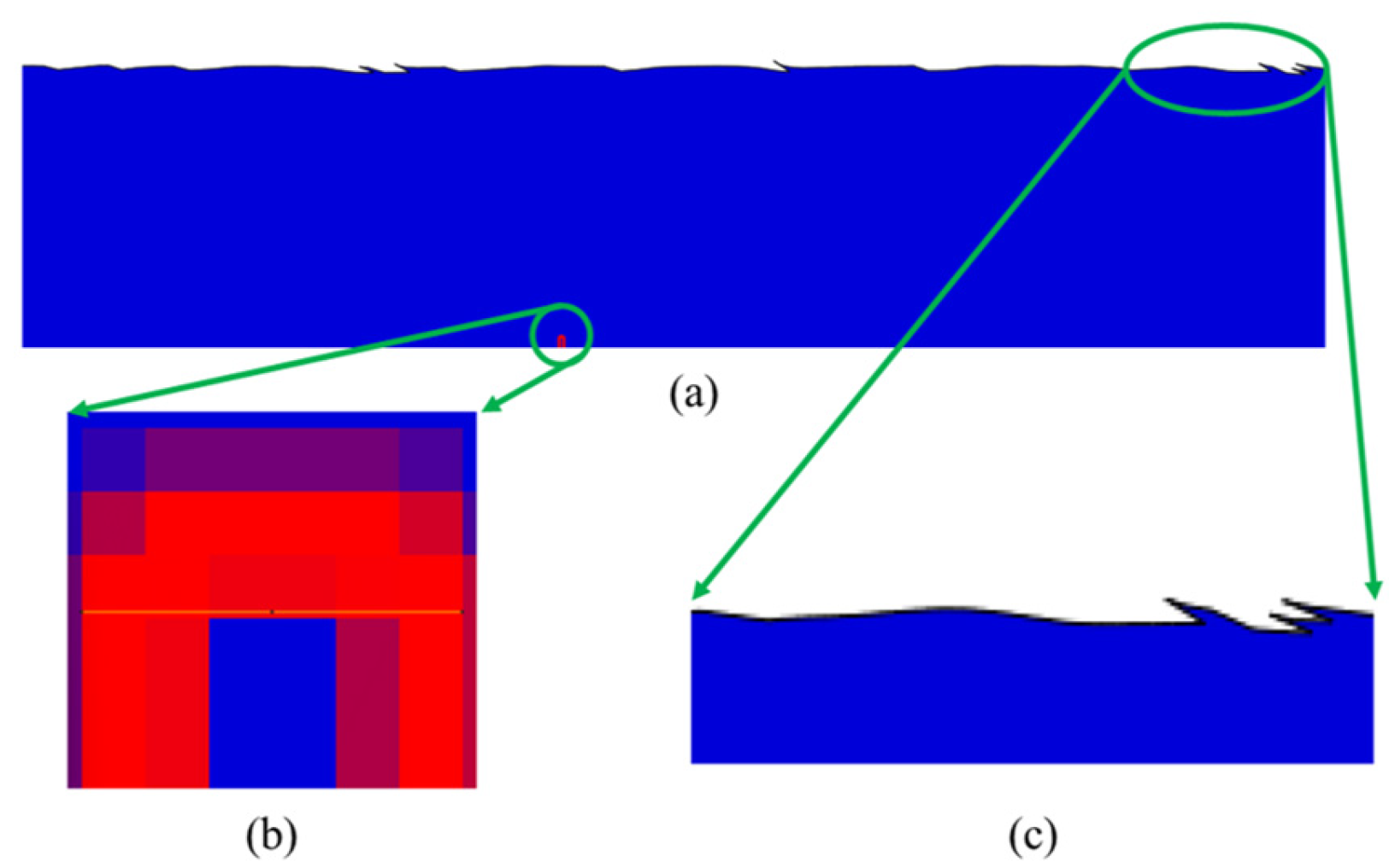
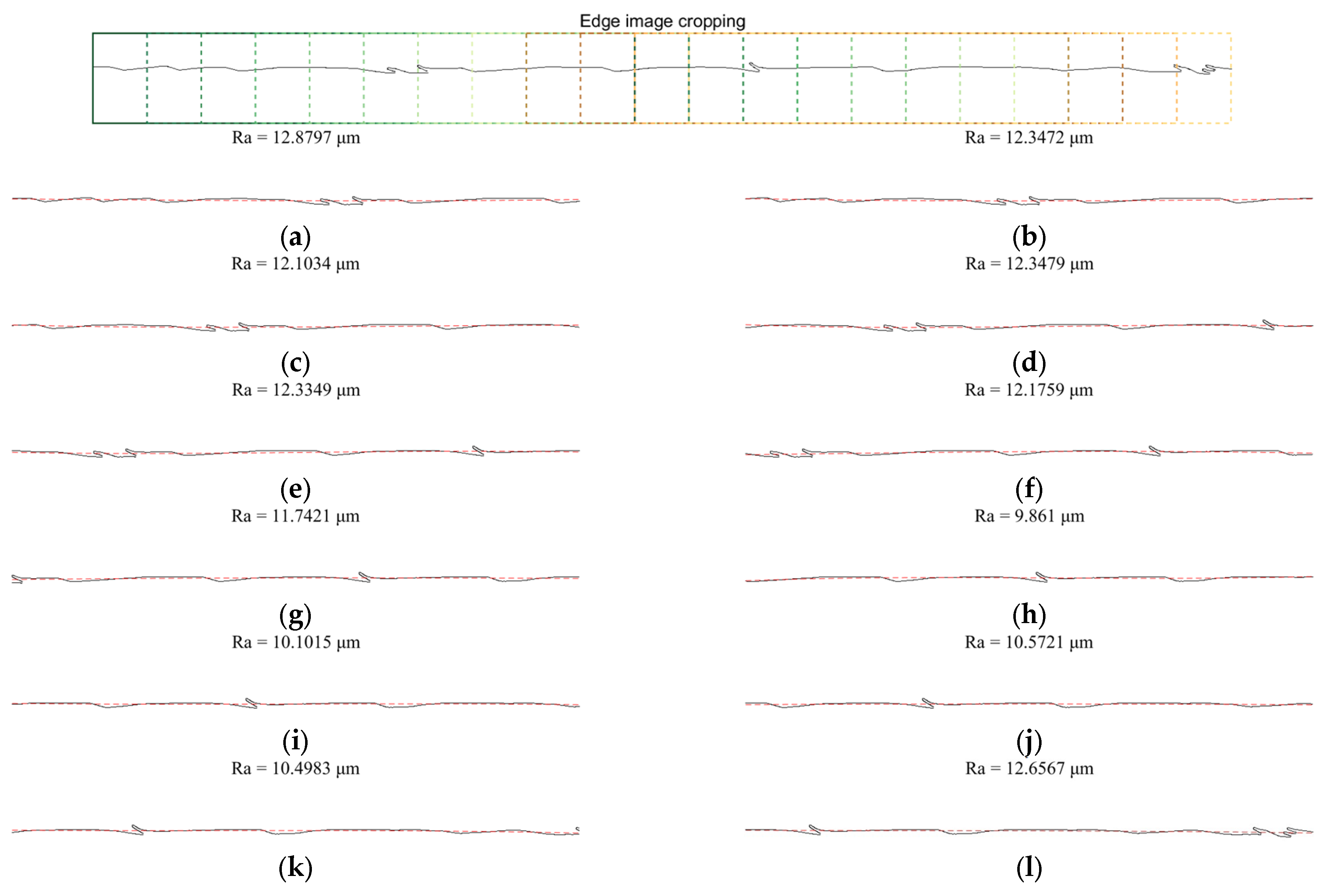
3.2. Workpiece Surface Characteristic Extraction

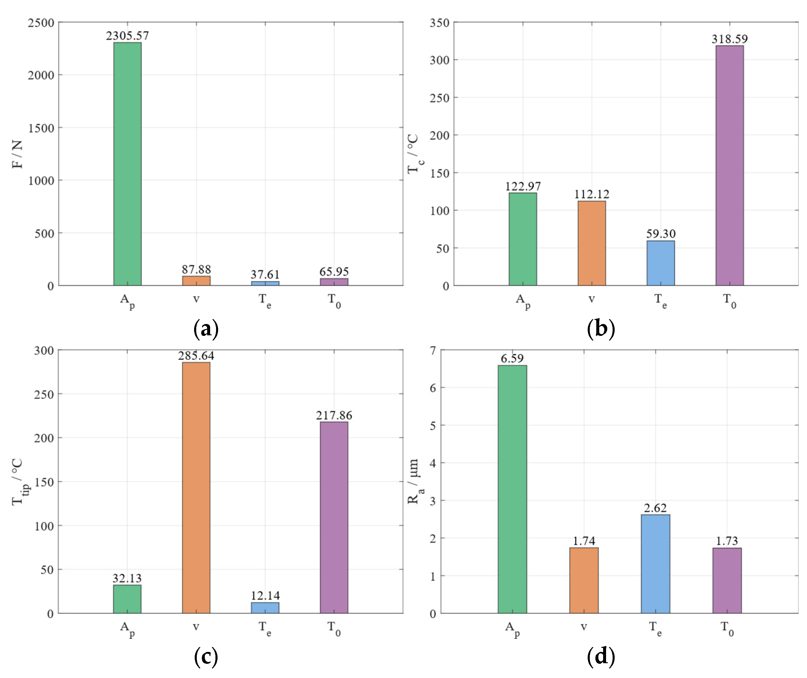
FES analysis not only not only provides insights into cutting force and cutting temperature but also enables the acquisition of surface properties of the workpiece, an aspect often overlooked in conventional research approaches, which typically rely on offline measurement [37]. Therefore, in this study, FES results were integrated with advanced image processing techniques to extract two-dimensional characteristic that describe the surface quality of the workpiece. The image processing method is illustrated in Figure 4. The processing method begins by marking a grid on the surface image of the workpiece after FES, as shown in Figure 5a. This grid served as a calibration point for image scaling, as demonstrated in Figure 5b. Once the pixel size of the calibration point is established, image processing techniques are employed to identify and measure the edge of the workpiece surface, facilitating the calculation of the surface roughness, as depicted in Figure 5c.

The extracted surface edge of the workpiece was used to calculate the arithmetic mean deviation $R_a$ of the workpiece surface using Equation (4):

$$R_a={\displaystyle \frac{1}{n}}{\sum }_{i=1}^n\left|z_i\right|,$$

(4)

where $n$ is the number of measured points located within the sampling length, and $z_i$ is the distance between the sampling point and the contour centerline. Following the roughness measurement technique, the procedure involved the initial extraction of surface images of the workpiece with a contour width of 5 mm. Afterwards, the contour centerline was computed through polynomial fitting (see the red dotted line in Figure 6), and $R_a$ was subsequently estimated using Equation (4). The measurement position was systematically shifted from left to right to cover the entire surface of the workpiece, and the average $R_a$ value was calculated. Figure 6 depicts the procedure for extracting and calculating the surface roughness map for test No. 8.

Through the image processing method, features were extracted for each experimental set, and the surface roughness $R_a$ was obtained, as shown in Table 6.

3.3. Range Analysis

Range analysis is a highly effective and straightforward method for analyzing and determining optimal combinations of parameters. Initially, the magnitudes of several factors at equal levels of cutting force, temperature, and surface roughness are computed using Equation (5) [38]:

$$\overline{K_{ij}}={\displaystyle \frac{{\Sigma }_j^4 M_{ij}}{4}},$$

(5)

where $M_{ij}$ represents the impact of factor $j$ on level $i$, and $\overline{K_{ij}}$ denotes the mean of $M_{ij}$. In this experiment, for each factor $j$, such as the cutting depth $A_p$, cutting speed $v$, ambient temperature $T_e$, and workpiece temperature $T_w$, four different levels were set. According to the FEM results in Table 4 and Table 5, there were four $M_{ij}$ values for each factor level, and $\overline{K_{ij}}$ is the mean calculated from the four $M_{ij}$ values. For example, when analyzing the impact of the four factors on the cutting force $F$, $\overline{K_{1j}}$ represents the impact value on the cutting force $F$ when factor $j$ is at the first level.

Then, the range $R_j$ for each factor mean $\overline{K_{ij}}$ is calculated in Equation (6):

$$R_j=\max \left\{ K_{1j},K_{2j},\dots ,K_{ij}\right\}-\min \left\{ K_{1j},K_{2j},\dots ,K_{ij}\right\},$$

(6)

A higher $R_j$ value indicates a more substantial influence of the factor on the experimental results, underscoring its significance. Consequently, $R_j$ can be used to analyse and identify the factors and corresponding levels that have the most substantial impact on a specific feature of interest. The calculation results of $R_j$ are presented in Figure 7.

The analysis in Figure 7 indicates that for the cutting force $F$, the most influential cutting parameter is the depth of cut $A_p$, followed by the cutting speed $v$ and initial temperature of the workpiece $T_0$, with the most negligible impact observed for the ambient temperature $T_e$. The optimal combination within the experimental range is $A_p=2 \mathrm{m}\mathrm{m}, v$ = $40 \mathrm{m}/\mathrm{m}\mathrm{i}\mathrm{n}$, $T_e=-5 °\mathrm{C}$, and $T_0$=$25 °\mathrm{C}$. For the temperature $T_c$ at the main cutting edge, the initial temperature $T_0$ has the highest impact, followed by the depth of cut $A_p$and the cutting speed $v$, with the most negligible influence from the ambient temperature $T_e$. The optimal combination is $A_p=1.5 \mathrm{m}\mathrm{m}, v$=$57 \mathrm{m}/\mathrm{m}\mathrm{i}\mathrm{n}$, $T_e=$40 °C, and $T_0=400 °\mathrm{C}$. The cutting speed $v$ has the most considerable impact on the temperature $T_{tip}$ at the tooltip, followed by the initial temperature $T_0$ and depth of cut $A_p$, with the least influence from ambient temperature $T_e.$ The optimal combination is $A_p=2 \mathrm{m}\mathrm{m}, v=57 \mathrm{m}/\mathrm{m}\mathrm{i}\mathrm{n}, T_e=25 °\mathrm{C},$ and$T_0=400 °\mathrm{C}$. Regarding the workpiece surface roughness $R_a$, the most influential factor is the depth of cut $A_p$, followed by the initial temperature $T_0$ and ambient temperature $T_e$, with the cutting speed $v$ having the least impact. The optimal combination is $A_p=2 \mathrm{m}\mathrm{m},v=40 \mathrm{m}/\mathrm{m}\mathrm{i}\mathrm{n},T_e=10°\mathrm{C},$ and $T_0=25 °\mathrm{C}$.

A comprehensive analysis of the experimental results indicates that increasing both cutting depth and speed leads to higher cutting forces and temperatures. This escalation simultaneously exacerbates system vibrations and instability, resulting in a decline in surface quality [38]. Integrating the insights from Figure 2 and Figure 3, it is evident that a greater cutting depth not only influences the size and shape of the chips but also accelerates their fracture time, promoting quicker dissipation of cutting heat. Additionally, an increase in cutting speed enhances the transfer of cutting heat to the chips, thereby reducing the temperature in the cutting zone. And, raising the cutting temperature of the workpiece and the ambient temperature can modify the material properties of the workpiece, reducing cutting resistance and pressure, which in turn lessens workpiece vibrations and improves surface quality. Therefore, selecting and combining the appropriate cutting depth, cutting speed, and thermal conditions helps enhance surface quality and improve machining efficiency.

3.4. Multiple Linear Regression Analysis

The multiple linear regression analysis (MLRA) method enables the precise representation of mathematical connection models with limited experiment data [39]. Therefore, based on the FES results analysed above, MLRA was employed to establish mathematical models for examining the relationship of cutting force, temperature, and workpiece surface roughness. This facilitates the optimization and selection of cutting parameters, enabling precise predictions of the machined surface quality. According to the classical empirical cutting force formulation [40], the turning force can be expressed in the exponential form of the cutting parameters as shown in Equation (7):

$$F=L{A_p}^{b_1}{v}^{b_2}{T_e}^{b_3}{T_0}^{b_4},$$

(7)

Here, $F$ represents the total cutting force. L, $b_1,b_2,b_3$, and $b_4$ are coefficients determined through the regression analysis. L is a coefficient related to the material, and $b_1,b_2,b_3$, and $b_4$ are the correction coefficients. The logarithm of Equation (8) gives:

$$lnF=C+b_{1}ln{A}_p+b_{2}lnv+b_{3}ln{T}_e+b_{4}ln{T}_0,$$

(8)

Let $lnF=y,{ x}_1=ln{A}_p, { x}_2=lnv, { x}_3=ln{T}_e, {and x}_4=ln{T}_w;$then, the MLR equation corresponding to Equation (9) is:

$$y=b_1{ x}_1+b_2{ x}_2+b_3{ x}_3+b_4{ x}_4,$$

(9)

The MLR in Equation (9) expresses the linear relationship between the independent variables ${ x}_1{, x}_2,{ x}_3,{\mathrm{a}\mathrm{n}\mathrm{d} x}_4$ and dependent variable $y$. Through the analysis of the 16 sets of simulation data in Section 3.3 and Section 3.4, the MLR formula was applied to the four independent variables. This resulted in expressions relating the cutting force $F$, cutting temperatures ($T_c,T_{tip}$), and surface roughness $R_a$ to the cutting parameters, as shown in Equation (10):

$$\begin{gathered} F=7.4788{A_p}^{0.7912}{v}^{0.0337}{T_e}^{0.0008}{T_0}^{-0.0037}, \\ {T}_c=2.7819{A_p}^{0.2945}{v}^{0.3638}{T_e}^{0.0171}{T_0}^{0.3232}, \\ {T}_{tip}=3.8806{A_p}^{0.0269}{v}^{0.528}{T_e}^{0.0037}{T_0}^{0.1131}, \\ {R}_a=1.8794{A_p}^{0.28035}{v}^{-0.11273}{T_e}^{-0.11162}{T_0}^{0.077811}. \end{gathered}$$

(10)

Validation of a multiple linear regression model (MLRM) is essential for ensuring its reliability and efficacy. Therefore, an R-squared ($R^2$) analysis of the MLRM was conducted to assist in evaluating the fitting quality, which stands for the determination coefficient of the MLRM.

$R^2$ is usually used to measure the extent to which a model explains the variability of the dependent variable in the MLRM. It ranges from 0 to 1, with a value closer to 1 indicating a higher ability of the model to explain the variability of the dependent variable, otherwise, the weaker it is. The calculation of R-squared [41] is given by Equations (11) and (12):

$$\overline{Ȳ}={\displaystyle \frac{1}{m}}{\sum }_{i=1}^m{Y}_i,$$

(11)

$$R^2=1-{\displaystyle \frac{{\sum }_{i=1}^m{\left(X_i-Y_i\right)}^2}{{\sum }_{i=1}^m{\left(\overline{Y}-Y_i\right)}^2}},$$

(12)

where $X_i$ is the predicted value of the $i^{th}$ regression model, while $Y_i$ corresponds to the $i^{th}$ value from FES results. $\overline{Ȳ}$ is the mean of the true values, and m denotes the total number of data points.

The coefficient of determination ($R^2$) results for the 16 tests are presented in Figure 8, where “Error” represents the relative discrepancy between model predictions and the training data from Table 5 and Table 6. The cutting force $F$ model within the MLRM achieves a particularly high degree of fit, with an $R^2$ value of 0.997 and an average relative error of 1.935. Models for the main cutting-edge temperature $T_c$ and tool tip temperature $T_{tip}$ also show substantial fit, with $R^2$ values of 0.856 and 0.897, and average relative errors of 14.808 and 6.341, respectively. Conversely, the regression model for surface roughness $R_a$ yields a comparatively lower fit, with an $R^2$ of 0.693 and an average relative error of 15.805. Nevertheless, the model’s overall trend aligns closely with the variations observed in the simulated experimental data, indicating that the MLRM established in this study can effectively predict the target parameters based on the results of FEA.

4. Turning Experiment Verification

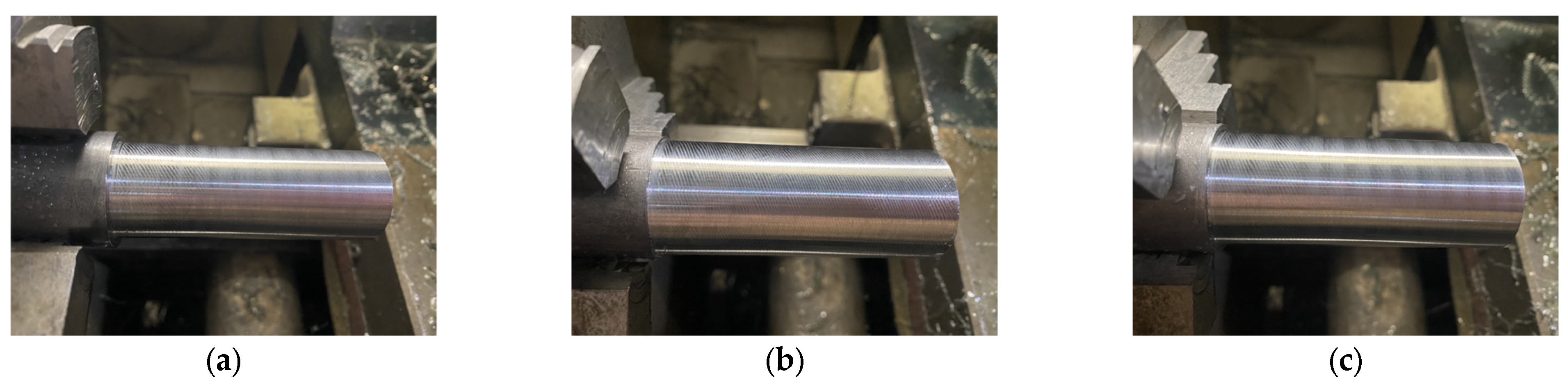
4.1. Turning Operation Description

Turning experiments were conducted using a CAK3665di CNC lathe with a power of 5.5 kW. To ensure experimental safety, the coolant was activated during the cutting process to cool the tool. An experimental levels table for the $L9(3³)$ orthogonal array with three factors and three levels was established to verify the impact of various variables, as shown in

Table 7. Experimental levels for the $L9(3³)$orthogonal array.

	Factor	${\mathit{A}}_{\mathit{p}} (\mathbf{m}\mathbf{m}$)	$\mathbf{v} (\mathbf{m}/\mathbf{m}\mathbf{i}\mathbf{n})$	$\mathit{f} (\mathbf{m}\mathbf{m}/\mathbf{r}\mathbf{e}\mathbf{v})$
Level
Level 1		1	127.2345	0.07
Level 2		2	152.6814	0.14
Level 3		3	178.1283	0.21

.

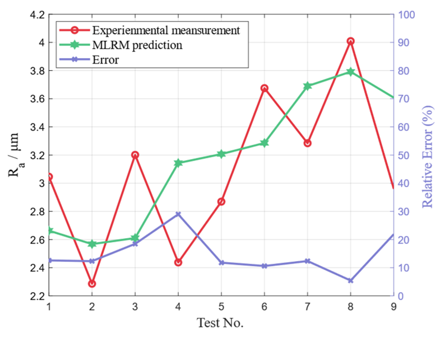
4.2. Workpiece Surface Roughness Measurement

After machining with different cutting parameters, the roughness of the workpiece surface was assessed using a roughness measurement instrument. Three positions, namely the end, middle, and tightened ends of the workpiece, were measured separately. Three measurements were performed at each position, and then the average values were recorded. The measurement results are presented in

Table 8. $L9\left(3^3\right)$ Cutting simulation results of the orthogonal experiment.

Test No.	${\mathit{A}}_{\mathit{p}} (\mathbf{m}\mathbf{m}$)	$\mathbf{v} (\mathbf{m}/\mathbf{m}\mathbf{i}\mathbf{n})$	$\mathit{f} (\mathbf{m}\mathbf{m}/\mathbf{r}\mathbf{e}\mathbf{v})$	${\mathit{R}}_{\mathit{a}}$$\left(\mathsf{\mu }\mathbf{m}\right)$
1	1	127.235	0.07	2.696
2	1	178.129	0.14	1.936
3	1	152.681	0.21	2.851
4	2	178.128	0.07	2.0873
5	2	152.681	0.14	2.519
6	2	127.235	0.21	3.325
7	3	152.681	0.07	2.934
8	3	127.235	0.14	3.659
9	3	178.128	0.21	2.61

.

Figure 9 shows the surface photographs following each sequential cut, progressing from the leftmost end to the rightmost end, with a cutting depth of 1 mm. The workpiece surface exhibited a vibrational texture caused by self-excited vibrations in the turning system. Notably, variations in surface texture were observed across workpieces of differing diameters, despite the use of identical cutting parameters. This observation further demonstrates the importance of online monitoring and prediction of the workpiece surface quality in real time during the turning process.

4.3. Experiment Result Analysis

To validate the accuracy of this method, the turning experiment parameters (Table 8) were combined with the MLRM established in Section 3.4 to predict the surface roughness $R_a$ of the workpiece under experimental conditions. Figure 10 compares the model’s predicted values and the actual experimental measurements. As depicted, the predicted trend closely follows the experimental trend: an increase in the depth of cut $A_p$ results in a corresponding increase in surface roughness $R_a$, while an increase in cutting speed $v$ leads to a decrease in $R_a$. Furthermore, the predictive model yields an average relative error of 14.928% against the experimentally measured values, indicating an accuracy of 85.072% for the MLRM model in predicting the $R_a$ value of the workpiece surface in the Q235B turning validation experiments.

5. Conclusions

This study proposes an innovative method for predicting workpiece surface quality by integrating finite element (FE) modeling with image processing techniques. Initially, an orthogonal experimental design was formulated based on commonly used cutting parameters and levels. Using these parameters, a finite element model of the cutting tool and workpiece was established to investigate the effects of cutting speed, cutting depth, workpiece temperature, and ambient temperature on cutting force, temperature in the cutting zone, and workpiece surface quality. The finite element analysis enabled the visualization of the cutting force, temperature, and surface conditions of the workpiece.

Subsequently, image processing techniques were applied to extract edge features from workpiece images generated through FEA. Polynomial fitting was used to quantify these edge features, and a calibration grid converted the image pixels into surface roughness values, enabling precise assessment of the actual surface roughness of the workpiece based on images.

To further analyze the impact of various cutting parameters on workpiece surface quality, a range analysis was conducted. The results indicated that cutting depth is the most significant factor affecting surface roughness, followed by workpiece temperature and ambient temperature, while cutting speed had the least effect. To quantify the relationships between cutting parameters, cutting force, temperature, and roughness, a multiple linear regression model was developed and validated using the R-squared ($R^2$) index.

Finally, an orthogonal experiment involving cutting depth, speed, and feed rate was conducted in an actual cutting environment to verify the effectiveness of this method. The measured workpiece surface roughness values under each experimental condition showed good consistency with the model’s predictions, achieving a prediction accuracy of 85.07%.

Despite these encouraging results of the proposed methodology, there are some limitations. Due to experimental and time constraints, this study utilized a three-factor, three-level orthogonal design, which did not encompass all cutting parameters. Additionally, a simplified 2D finite element model was employed to reduce computational time, potentially impacting the accuracy of the simulation results. Future research should consider a more comprehensive set of cutting parameters and explore the development of a 3D finite element model to enhance the accuracy and generalizability of the model. Furthermore, while the roughness measurement standard used in this study is the Chinese standard GB/T 1031-2009 [42], future work should consider incorporating international standards to broaden the applicability of the results.

References

1. Bian, H.; Wang, Z.; Zhang, H.; Bu, X.; Lu, H.; Luo, K.; Lu, J. Response Surface Methodology-Based Optimization of Parameters and Cutting Quality of 22MnB5 Plates by UV Picosecond Laser Layered Cutting. Opt. Laser Technol. 2024, 177, 111197. [Google Scholar] [CrossRef]
2. Cui, Z.; Liu, H.; Wu, L.; Cao, Z.; Zong, W. Cutting Force and Surface Quality in Ultra-Precision Milling of Oxygen-Free Copper under Different Cutting Strategies. J. Manuf. Process. 2024, 131, 2420–2442. [Google Scholar] [CrossRef]
3. Wu, P.; He, Y.; Li, Y.; He, J.; Liu, X.; Wang, Y. Multi-Objective Optimisation of Machining Process Parameters Using Deep Learning-Based Data-Driven Genetic Algorithm and TOPSIS. J. Manuf. Syst. 2022, 64, 40–52. [Google Scholar] [CrossRef]
4. Wang, L.; Yue, C.; Liu, X.; Li, M.; Xu, Y.; Liang, S.Y. Conventional and Micro Scale Finite Element Modeling for Metal Cutting Process: A Review. Chin. J. Aeronaut. 2023, 37, 199–232. [Google Scholar] [CrossRef]
5. Nomani, J.; Polishetty, A.; Hilditch, T.; Littlefair, G. Developing a 2D Finite Element Cutting Model Based on Individual Phases in Orthogonal Cutting of Two-Phase Duplex Stainless Steel. Mater. Today Proc. 2023. [Google Scholar] [CrossRef]
6. Li, C.; Shi, D.; Li, B.; Wang, H.; Feng, G.; Gu, F.; Ball, A.D. Modelling the Dynamics of a CNC Spindle for Tool Condition Identification Based on On-Rotor Sensing. Mech. Mach. Sci. 2023, 117, 1057–1071. [Google Scholar] [CrossRef]
7. Vijayaraghavan, V.; Garg, A.; Gao, L.; Vijayaraghavan, R.; Lu, G. A Finite Element Based Data Analytics Approach for Modeling Turning Process of Inconel 718 Alloys. J. Clean. Prod. 2016, 137, 1619–1627. [Google Scholar] [CrossRef]
8. Ye, G.G.; Jiang, M.Q.; Xue, S.F.; Ma, W.; Dai, L.H. On the Instability of Chip Flow in High-Speed Machining. Mech. Mater. 2018, 116, 104–119. [Google Scholar] [CrossRef]
9. Yue, C.; Liu, X.; Liu, Z.; Xie, N.; Wang, Y. Tool Optimization for Splicing Die Milling Processes Based on Finite Element Simulation. Chin. Mech. Eng. 2020, 31, 2085–2094. [Google Scholar]
10. Muhammad, R.; Roy, A.; Silberschmidt, V.V. Finite Element Modelling of Conventional and Hybrid Oblique Turning Processes of Titanium Alloy. Procedia CIRP 2013, 8, 510–515. [Google Scholar] [CrossRef]
11. Okokpujie, I.P.; Tartibu, L.K.; Chima, P.C.; Ogundipe, A.T. A Finite Element Based Investigation of Tool Wear Rate via Machining of Al6061 Alloys Using Deform-3D. Mater. Today Proc. 2023. [Google Scholar] [CrossRef]
12. Gok, K. Development of Three-Dimensional Finite Element Model to Calculate the Turning Processing Parameters in Turning Operations. Measurement 2015, 75, 57–68. [Google Scholar] [CrossRef]
13. Fetecau, C.; Stan, F. Study of Cutting Force and Surface Roughness in the Turning of Polytetrafluoroethylene Composites with a Polycrystalline Diamond Tool. Measurement 2012, 45, 1367–1379. [Google Scholar] [CrossRef]
14. Pan, L.; Wu, Z.R.; Fang, L.; Song, Y.D. Investigation of Surface Damage and Roughness for Nickel-Based Superalloy GH4169 under Hard Turning Processing. Proc. Inst. Mech. Eng. Part B J. Eng. Manuf. 2020, 234, 679–691. [Google Scholar] [CrossRef]
15. Jia, S.; Wang, S.; Li, S.; Cai, W.; Liu, Y.; Bai, S.; Li, Z.S. Integrated Multi-Objective Optimization of Rough and Finish Cutting Parameters in Plane Milling for Sustainable Machining Considering Efficiency, Energy, and Quality. J. Clean. Prod. 2024, 471, 143406. [Google Scholar] [CrossRef]
16. Wang, Y.; Xu, K.; Xue, H.; Li, J.; Li, Y. Anisotropic Mechanism of Monocrystalline Silicon on Surface Quality in Precision Diamond Wire Saw Cutting. Mater. Sci. Semicond. Process 2025, 185, 108961. [Google Scholar] [CrossRef]
17. Li, K.; Wang, X.; Gu, L. Magnetic Field Assisted Blasting Erosion Arc Machining (M-BEAM): A Novel Efficient and Quality Improved Machining Method for Inconel 718. J. Manuf. Process. 2024, 131, 233–244. [Google Scholar] [CrossRef]
18. Wang, P.; Tao, H.; Qi, J.; Li, P. Machining Quality Prediction of Complex Thin-Walled Parts Using Multi-Task Dual Domain Adaptive Deep Transfer Learning. Adv. Eng. Inform. 2024, 62, 102640. [Google Scholar] [CrossRef]
19. Liu, C.; Xu, W.; Niu, T.; Chen, Y. Roughness Evolution of Constrained Surface Based on Crystal Plasticity Finite Element Model and Coupled Eulerian-Lagrangian Method. Comput. Mater. Sci. 2022, 201, 110900. [Google Scholar] [CrossRef]
20. Ma, X.; Zhao, J.; Du, W.; Zhang, X.; Jiang, Z. Analysis of Surface Roughness Evolution of Ferritic Stainless Steel Using Crystal Plasticity Finite Element Method. J. Mater. Res. Technol. 2019, 8, 3175–3187. [Google Scholar] [CrossRef]
21. Yang, J.; Wang, X.; Kang, M. Finite Element Simulation of Surface Roughness in Diamond Turning of Spherical Surfaces. J. Manuf. Process. 2018, 31, 768–775. [Google Scholar] [CrossRef]
22. Zhang, X.; Zheng, G.; Cheng, X.; Li, Y.; Li, L.; Liu, H. 2D Fractal Analysis of the Cutting Force and Surface Profile in Turning of Iron-Based Superalloy. Measurement 2020, 151, 107125. [Google Scholar] [CrossRef]
23. Zhou, Y.; Wang, S.; Chen, H.; Zou, J.; Ma, L.; Yin, G. Study on Surface Quality and Subsurface Damage Mechanism of Nickel-Based Single-Crystal Superalloy in Precision Turning. J. Manuf. Process. 2023, 99, 230–242. [Google Scholar] [CrossRef]
24. Zheng, G.; Xu, R.; Cheng, X.; Zhao, G.; Li, L.; Zhao, J. Effect of Cutting Parameters on Wear Behavior of Coated Tool and Surface Roughness in High-Speed Turning of 300M. Measurement 2018, 125, 99–108. [Google Scholar] [CrossRef]
25. Liu, W.; Yang, X.; Zhang, P.; Chen, Y. Prediction Model of Surface Roughness of 7055 Aluminum Alloy after High Speed Cutting. Ordnance Mater. Sci. Eng. 2015, 38, 1–4. [Google Scholar] [CrossRef]
26. Xi, Y.; Bermingham, M.; Wang, G.; Dargusch, M. FEA Modelling of Cutting Force and Chip Formation in Thermally Assisted Machining of Ti6Al4V Alloy. Mater. Sci. Forum 2013, 765, 343–347. [Google Scholar] [CrossRef]
27. GB/T 700-2006; Carbon Structural Steels. ISO 630:1995, Structural Steels-Plates, Wide Flats, Bars, Sections and Profiles, NEQ. General Administration of Quality Supervision, Inspection and Quarantine of the People’s Republic of China: Beijing, China, 2006.
28. ISO 21920-2:2021; Geometrical Product Specifications (GPS)—Surface Texture: Profile—Part 2: Terms, Definitions and Surface Texture Parameters. ISO: Geneva, Switzerland, 2021.
29. Lin, L.; Zhi, X.D.; Fan, F.; Meng, S.J.; Su, J.J. Determination of Parameters of Johnson-Cook Models of Q235B Steel. J. Vib. Shock 2014, 33, 153–158. [Google Scholar]
30. Zhang, Y.; Jia, Y.; Wang, S.S.Y. An Improved Nearly-Orthogonal Structured Mesh Generation System with Smoothness Control Functions. J. Comput. Phys. 2012, 231, 5289–5305. [Google Scholar] [CrossRef]
31. Garimella, R.V. Mesh Data Structure Selection for Mesh Generation and FEA Applications. Int. J. Numer. Methods Eng. 2002, 55, 451–478. [Google Scholar] [CrossRef]
32. Smolenicki, D.; Boos, J.; Kuster, F.; Roelofs, H.; Wyen, C.F. In-Process Measurement of Friction Coefficient in Orthogonal Cutting. CIRP Ann. Manuf. Technol. 2014, 63, 97–100. [Google Scholar] [CrossRef]
33. Usluer, E.; Emiroğlu, U.; Yapan, Y.F.; Kshitij, G.; Khanna, N.; Sarıkaya, M.; Uysal, A. Investigation on the Effect of Hybrid Nanofluid in MQL Condition in Orthogonal Turning and a Sustainability Assessment. Sustain. Mater. Technol. 2023, 36, e00618. [Google Scholar] [CrossRef]
34. Zhang, Y.; Wu, M.; Liu, K.; Zhang, J. Optimization of Surface Roughness and Machining Parameters for Turning Superalloy GH4169 under High-Pressure Cooling. Surf. Topogr. 2021, 9, 045045. [Google Scholar] [CrossRef]
35. Li, C.; Zou, Z.; Duan, W.; Liu, J.; Gu, F.; Ball, A.D. Characterizing the Vibration Responses of Flexible Workpieces during the Turning Process for Quality Control. Appl. Sci. 2023, 13, 12611. [Google Scholar] [CrossRef]
36. Cui, Z.; Ni, J.; He, L.; Su, R.; Wu, C.; Xue, F.; Sun, J. Assessment of Cutting Performance and Surface Quality on Turning Pure Polytetrafluoroethylene. J. Mater. Res. Technol. 2022, 20, 2990–2998. [Google Scholar] [CrossRef]
37. Liu, C.; Huang, Z.; Huang, S.; He, Y.; Yang, Z.; Tuo, J. Surface Roughness Prediction in Ball Screw Whirlwind Milling Considering Elastic-Plastic Deformation Caused by Cutting Force: Modelling and Verification. Measurement 2023, 220, 113365. [Google Scholar] [CrossRef]
38. Meraz, M.; Alvarez-Ramirez, J.; Rodriguez, E. Multivariate Rescaled Range Analysis. Phys. A Stat. Mech. Its Appl. 2022, 589. [Google Scholar] [CrossRef]
39. Çelik, Y.H.; Fidan, Ş. Analysis of Cutting Parameters on Tool Wear in Turning of Ti-6Al-4V Alloy by Multiple Linear Regression and Genetic Expression Programming Methods. Measurement 2022, 200, 111638. [Google Scholar] [CrossRef]
40. Black, S.C.; Chiles, V.; Lissaman, A.J.; Martin, S.J. Turning and Milling. In Principles of Engineering Manufacture, 3rd ed.; Butterworth-Heinemann: Oxford, UK, 1996; pp. 316–371. [Google Scholar] [CrossRef]
41. Chicco, D.; Warrens, M.J.; Jurman, G. The Coefficient of Determination R-Squared Is More Informative than SMAPE, MAE, MAPE, MSE and RMSE in Regression Analysis Evaluation. PeerJ Comput. Sci. 2021, 7, e623. [Google Scholar] [CrossRef]
42. GB/T 1031-2009; Geometrical Product Specifications(GPS)-Surface Texture: Profile Method-Surface Roughness Parameters and Their Values. General Administration of Quality Supervision, Inspection and Quarantine of the People’s Republic of China: Beijing, China, 2009.
Figure 1. FEM of turning process: (a) mesh model and (b) tool cutting edge.
Machines 12 00827 g001
Figure 2. Cutting mises cloud maps of test (a) No. 1, (b) No. 7, (c) No. 10, and (d) No. 16.
Machines 12 00827 g002
Figure 3. Cutting temperature cloud maps of test (a) No. 1, (b) No. 7, (c) No. 10, and (d) No. 16.
Machines 12 00827 g003aMachines 12 00827 g003b
Figure 4. Flowchart of workpiece surface feature extraction.
Machines 12 00827 g004
Figure 5. (a) Workpiece surface from FES, (b) enlarged reference mesh grid, and (c) enlarged local workpiece surface.
Machines 12 00827 g005
Figure 6. Extraction of the workpiece surface edge for Test No. 8: (a) measuring position 1, (b) measuring position 2, (c) measuring position 3, (d) measuring position 4, (e) measuring position 5, (f) measuring position 6, (g) measuring position 7, (h) measuring position 8, (i) measuring position 9, (j) measuring position 10, (k) measuring position 11, and (l) measuring position 12.
Machines 12 00827 g006
Figure 7. Result of range analysis, R j of (a) F , (b) T c , (c) T t i p , and (d) R a .
Machines 12 00827 g007
Figure 8. Coefficient of determination ( R 2 ) for (a) F , (b) T c , (c) T t i p , and (d) R a in the MLRM.
Machines 12 00827 g008aMachines 12 00827 g008b
Figure 9. Workpiece surface after each cut: (a) cutting diameter from 34.91 mm to 32.94 mm, (b) cutting diameter from 32.94 mm to 30.93 mm, and (c) cutting diameter from 30.93 mm to 29.01 mm.
Machines 12 00827 g009
Figure 10. Comparison of R a between prediction of MLRM and experimental measurements.
Machines 12 00827 g010