Design of a Path-Tracking Controller with an Adaptive Preview Distance Scheme for Autonomous Vehicles

Abstract

This paper presents a method to design a path-tracking controller with an adaptive preview distance scheme for autonomous vehicles. Generally, the performance of a path-tracking controller depends on tire–road friction and is severely deteriorated on low-friction roads. To cope with the problem, it is necessary to design a path-tracking controller that is robust against variations in tire–road friction. In this paper, a preview function is introduced into the state-space model built for better path-tracking performance. With the preview function, an adaptive preview distance scheme is proposed to adaptively adjust the preview distance according to the variations in tire–road friction. Front-wheel steering (FWS) and four-wheel steering (4WS) are adopted as actuators for path tracking. With the state-space model, a linear quadratic regulator (LQR) is adopted as a controller design methodology. In the adaptive preview distance scheme, the best preview distance is obtained from simulation for several tire–road friction conditions. Curve fitting with an exponential function is applied to those preview distances with respect to the tire–road friction. To verify the performance of the adaptive preview distance scheme under variations in tire–road friction, a simulation is conducted on vehicle simulation software. From the simulation results, it was shown that the path-tracking controller with an adaptive preview distance scheme presented in this paper was effective for path tracking against variations in tire–road friction in the peak’s center offset, and the settling delays were reduced by 60% and 23%, respectively.

1. Introduction

For the last decade, autonomous driving has been known as a next-generation solution for future transportation in research institutes and the automotive industry because it can reduce several types of traffic accidents and make road safety and traffic flow better [1,2,3]. For example, it was shown that a human driver with an excessive acceleration or braking style has a significant harmful impact on fuel consumption and emission pollutions [4]. For those reasons, autonomous driving is considered as a potential alternative for the current transportation system problems. From the literature survey, it is well known that a generic modular system architecture for autonomous driving consists of detection, localization, prediction, planning, and control. Among them, localization, prediction, planning, and control can be merged into a single step, called end-to-end driving [2]. Among these topics, path-tracking control (PTC) has been widely studied. Consequently, a great number of papers have been published in the research area of PTC [5,6,7,8,9,10,11,12,13]. In this paper, it is assumed that PTC aims at the level 5 of autonomous driving [14].

Generally, most of the PTC proposed to date has been designed on high-friction roads. Although this has shown good path-tracking performance on high-friction roads, it does not hold on low-friction roads [15,16,17]. This means that the tire–road friction coefficient, μ, has a significant influence on the path-tracking performance. More specifically, this is caused by the fact that the lateral tire force becomes much smaller due to low μ conditions. Another problem, due to the same reason, is that several actuator combinations, such as front-wheel steering (FWS), four-wheel steering (4WS), and four-wheel independent braking/driving (4WIB/4WID), have little influences on the path-tracking performance [16,17]. In the opposite case, a PTC designed on low μ roads also shows poor path-tracking performance on high μ ones due to the longer preview distance under low μ conditions. In other words, on high μ roads, for better path tracking, it needs a smaller preview distance than that needed on low μ roads.

To cope with the problem caused by the variations in μ, several methods have been proposed to date. As the most popular one, gain scheduling has been selected for PTC under various operating conditions [18,19,20,21,22,23,24,25,26,27]. This method designs several controllers at several fixed points of time-varying parameters, and then interpolates or linearly combines those controllers over a range of time-varying ones. Finally, if a current point is identified or estimated, the corresponding controller is selected from interpolation or linear combination and is applied to PTC. Most papers using gain scheduling adopted vehicle speed and its inverse as a scheduling variable. On the contrary, there are few papers that selected μ as a scheduling variable.

An adaptive control has also been used as a robust controller for PTC [28,29,30,31,32,33,34,35,36]. This method of control changes controller gains according to variations in vehicle speed, cornering stiffness, and μ. In this method, those parameters related to PTC are estimated by parameter adaptation schemes, such as recursive-least-square (RLS) or neural networks [31,32,36]. Then, the estimated parameters are directly used in a controller. The drawback of adaptive control is that a parameter adaptation scheme is needed for the controller, and the control performance highly depends on the speed and accuracy of parameter adaptation. Gain scheduling and adaptive control have been combined with H_∞ control, MPC, and SMC [18,19,21,22,23,24,25,27,31,34].

When coping with the parameter variations, such as vehicle speed and μ, the simplest method is to adopt adaptive look-ahead or preview distance schemes [37,38,39,40,41,42]. In those papers, a preview distance was adaptively adjusted using fuzzy reasoning according to parameter variations. The vehicle speed, side-slip angle, yaw rate, and road curvature were fed into the fuzzy membership function, and the preview distance or the velocity gain was obtained by fuzzy reasoning. However, most of those papers selected the vehicle speed as a scheduling variable, except in [41]. In this paper, μ is selected as a scheduling parameter.

In this paper, a state-space model is obtained from the target path and 2-DOF bicycle model [16,17,18,19,20,21,23,24,25,26,27,31,32,33,34,35,36,38,42,43]. This state-space model has the state variables of the lateral offset and heading errors, the side-slip angle, and the yaw rate. Using the state-space model, LQR is designed in this paper [16,17,18,20,26,43]. For LQR design, the LQ objective function with weights on the state variables is defined. The input configurations of LQR are FWS and 4WS, which are easily represented in the state-space model [16,17,43]. To improve the path-tracking performance, the constraints on tire-slip angles are applied [43].

To cope with the variations in μ, an adaptive preview distance scheme (APDS) is proposed in this paper. The APDS consists of three consecutive steps. The first step is to design the LQR on the road, where μ is 0.8. The second step is to tune the preview distance using the gain of LQR obtained from the first step in order to obtain the best path-tracking performance for each μ, divided from 0.3 to 0.8 with an interval of 0.1. The third step is to apply curve fitting with an exponential function to those preview distances with respect to μ. Those steps are performed through simulation using vehicle simulation software. A double-lane-change maneuver for collision avoidance is selected as a test scenario [16,17,26,38,43]. A notable feature is that a fixed gain is used when tuning the preview distances for several μ conditions. The only tuning parameter is the preview distance or the velocity gain. For this reason, this method is quite simple, compared to the previously proposed methods that used fuzzy reasoning.

The contributions of this paper can be summarized as follows:

• This paper presents an adaptive preview distance scheme in order to overcome the problem caused by the variations in μ. This method is quite simple, compared to the previously proposed methods.
• FWS and 4WS are used as actuators for PTC in this paper. With those steering actuators, the effects of various actuators on the adaptive preview distance scheme and path-tracking performance are investigated.

This paper has five sections. Section 2 describes the vehicle model and LQR design procedures for PTC. The APDS is also presented in this section. In Section 3, measures used to evaluate performance are presented. Simulation is performed and the results are analyzed in Section 4. Conclusions are drawn in Section 5.

2. Design of a Path-Tracking Controller with an Adaptive Preview Distance Scheme

In this paper, an LQR that uses full-state feedback was selected as a PTC. Using the state-space model and the LQ objective function, the LQR was designed. To maximize the lateral tire forces on low μ roads, constraints were imposed on the front and rear steering angles. With LQR, the APDS was proposed.

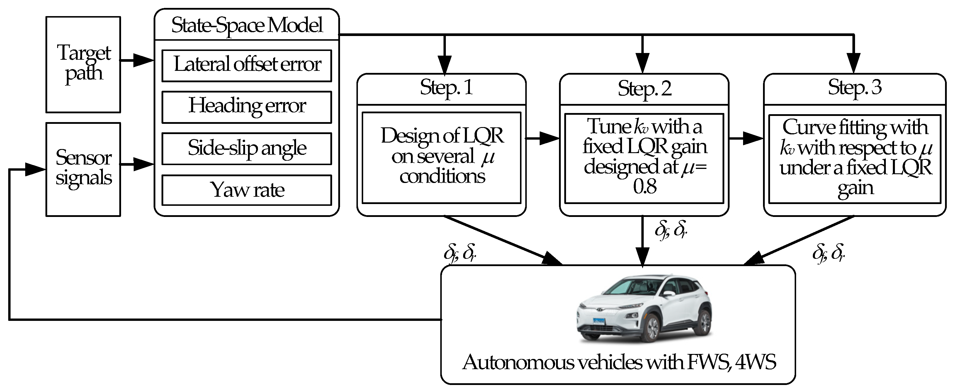
Figure 1 shows the schematic diagram of the path-tracking controller with the APDS proposed in this paper. As shown in Figure 1, the proposed APDS consisted of three steps. The first step was to design the LQR on several μ conditions. The second step was to tune the preview distance or the velocity gain, k_v, with a fixed LQR gain, designed on the road where μ was 0.8. The third step was to apply curve fitting to k_v with respect to μ.

2.1. Derivation of State-Space Model

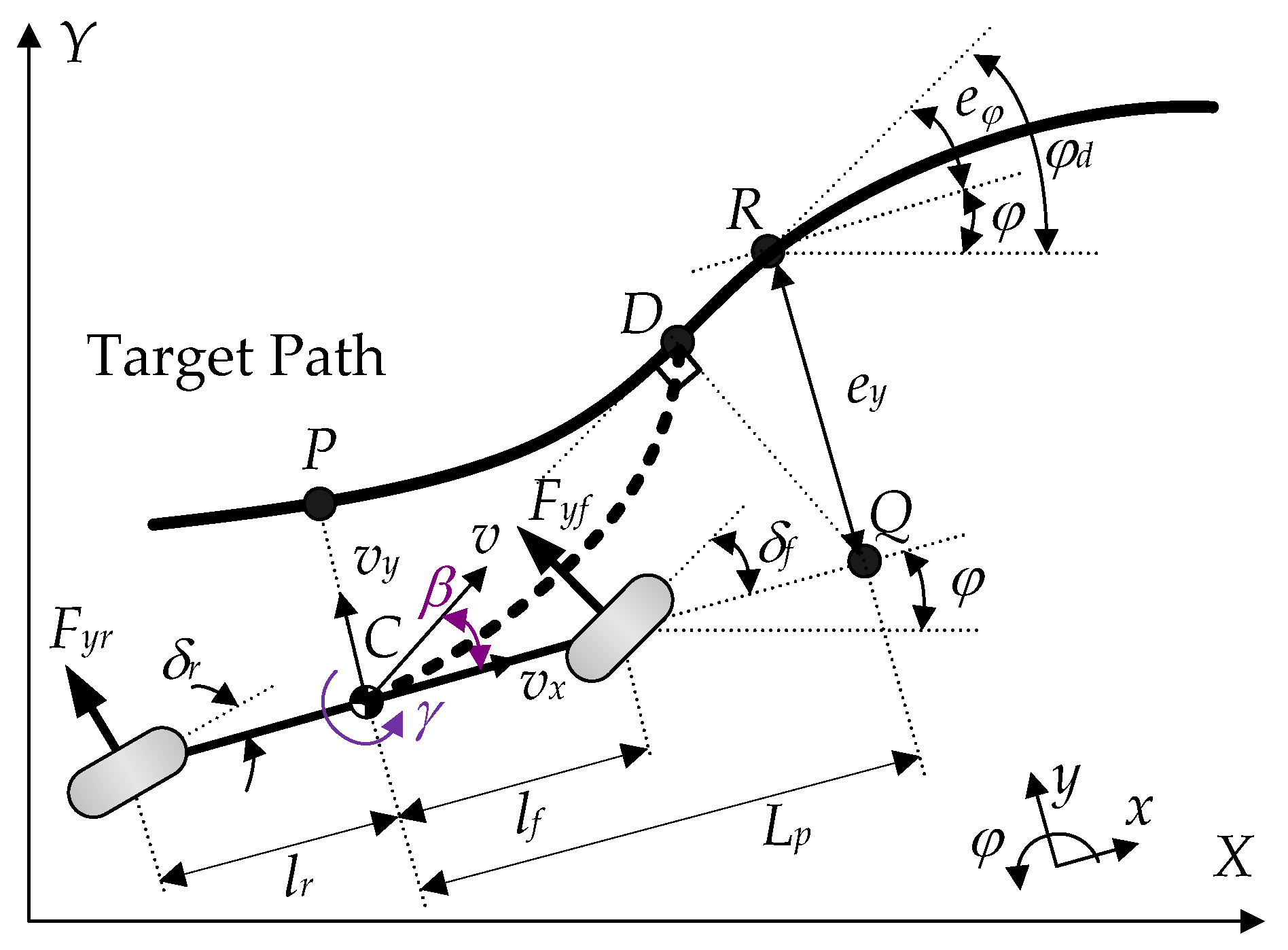
In the context of PTC, a 2-DOF bicycle model was selected to represent a vehicle, as discussed in the literature [16,17,18,19,20,21,23,24,25,26,27,31,32,33,34,35,36,38,42,43]. Figure 2 outlines the coordinates and variables used to describe this model, along with the target path for path tracking. This model is focused on modeling the yaw and lateral motions of a vehicle while assuming a constant longitudinal velocity, v_x. The state variables were the yaw rate, γ, and the side-slip angle, β, which is defined as the ratio between the longitudinal and lateral velocities. The equations of motion (1) were established [16,17]. The tire-slip angles, κ_f and κ_r, at the front and rear wheels were defined, as in (2), and the calculation of linear lateral tire forces, F_yf and F_yr, is detailed in (3). By combining (1), (2), and (3), the time derivatives of the state variables for the bicycle model were derived, as in (4).

$$\left\{\begin{array}{l}m{v}_x\left(\dot{\beta }+\gamma \right)=F_{yf}+F_{yr}\\ I_z\dot{\gamma }=l_f{F}_{yf}-l_r{F}_{yr}\end{array}\right.$$

(1)

$${\kappa }_f={\delta }_f-\beta -{\displaystyle \frac{l_f\gamma }{v_x}},\hspace{1em}{\kappa }_r={\delta }_r-\beta +{\displaystyle \frac{l_r\gamma }{v_x}}$$

(2)

$$F_{yf}=C_f{\kappa }_f,\hspace{1em}{F}_{yr}=C_r{\kappa }_r$$

(3)

$$\begin{array}{l}\dot{\beta }=\left({\displaystyle \frac{{\varsigma }_1}{m{v}_x}}\right)\beta +\left({\displaystyle \frac{{\varsigma }_2}{m{v}_x^2}}-1\right)\gamma +{\displaystyle \frac{C_f}{m{v}_x}}{\delta }_f+{\displaystyle \frac{C_r}{m{v}_x}}{\delta }_r\\ \dot{\gamma }=\left({\displaystyle \frac{{\varsigma }_2}{I_z}}\right)\beta +\left({\displaystyle \frac{{\varsigma }_3}{I_z{v}_x}}\right)\gamma +{\displaystyle \frac{l_f{C}_f}{I_z}}{\delta }_f-{\displaystyle \frac{l_r{C}_r}{I_z}}{\delta }_r\\ {\varsigma }_1=-C_f-C_r,\hspace{0.33em}{\varsigma }_2=-C_f{l}_f+C_r{l}_r,\hspace{0.33em}{\varsigma }_3=-l_f^2{C}_f-l_r^2{C}_r\end{array}$$

(4)

The literature on PTC introduces the lateral offset error, e_y, and the heading error, e_φ, at the point P, as shown in Figure 2. For better path-tracking performance, this paper adopted a look-ahead or preview function, drawing upon the work of various researchers [37,38,39,40,41,42,43]. The preview distance, L_p, was determined, as in (5). Here, k_v is a velocity gain, which stands for the preview interval. The adaptive preview distance scheme proposed in this paper is to tune k_v according to the variations in μ. In Figure 2, point C corresponds to the center of gravity (C.G.). The preview point, labeled as Q, and the point R on the target path were determined based on the computed look-ahead distance, L_p. At the point R, the time derivatives of the errors, e_y and e_φ, were calculated, as in (6), while assuming that e_φ was limited to be less than 10° and, accordingly, was approximated as sine_φ ≈ e_φ:

$$L_p=k_v\cdot v_x$$

(5)

$$\left\{\begin{array}{l}{\dot{e}}_y=v_x\sin e_{\phi }-v_x\beta -L_p\gamma \approx v_x{e}_{\phi }-v_x\beta -L_p\gamma \\ {\dot{e}}_{\phi }={\dot{\phi }}_d-\dot{\phi }=v_x\chi -\gamma \end{array}\right.$$

(6)

Utilizing the state variables e_y, e_φ, β, and γ, the state vector, x, the disturbance, w, and control input, u, were established, as in (7). The state-space equation for the path-tracking control system, as presented in (8), is a result of the integration of (4), (6), and (7). Within (8), the matrices for the system, the disturbance, and the control input are denoted by A, B₁, and B₂:

$$x={\left[\begin{array}{cccc}{e}_y& e_{\phi }& \beta & \gamma \end{array}\right]}^T,\hspace{1em}w=\chi ,\hspace{1em}u={\left[\begin{array}{cc}{\delta }_f& {\delta }_r\end{array}\right]}^T$$

(7)

$$\dot{x}=Ax+B_{1}w+B_{2}u$$

(8)

$$A=\left[\begin{array}{cccc}0& v_x& -v_x& -L_p\\ 0& 0& 0& -1\\ 0& 0& {\displaystyle \frac{{\varsigma }_1}{m{v}_x}}& {\displaystyle \frac{{\varsigma }_2}{m{v}_x^2}}-1\\ 0& 0& {\displaystyle \frac{{\varsigma }_2}{I_z}}& {\displaystyle \frac{{\varsigma }_3}{I_z{v}_x}}\end{array}\right],\hspace{1em}{B}_1=\left[\begin{array}{c}0\\ v_x\\ 0\\ 0\end{array}\right],\hspace{1em}{B}_2=\left[\begin{array}{ll}0\hfill & 0\hfill \\ 0\hfill & 0\hfill \\ {\displaystyle \frac{C_f}{m{v}_x}}\hfill & {\displaystyle \frac{C_r}{m{v}_x}}\hfill \\ {\displaystyle \frac{l_f{C}_f}{I_z}}\hfill & -{\displaystyle \frac{l_r{C}_r}{I_z}}\hfill \end{array}\right]$$

(9)

The control input, denoted as u in (7), comprises two elements: front steering angle, δ_f, and rear steering angle, δ_r. These elements were used to define two distinct control inputs, u_FWS and u_4WS, corresponding to input configurations, FWS and 4WS. Derived from (9), the input matrices B_2,FWS and B_2,4WS were determined, as in (10), with B₂(i) representing the i-th column of matrix B₂ [16]:

$$\left\{\begin{array}{lll}{u}_{\mathrm{FWS}}={\delta }_f\hfill & B_{2,\mathrm{FWS}}=\left[B_2\left(1\right)\right]\hfill & \mathrm{for}\hspace{0.33em}\mathrm{FWS}\hfill \\ u_{4\mathrm{WS}}={\left[\begin{array}{cc}{\delta }_f& {\delta }_r\end{array}\right]}^T\hfill & B_{2,4\mathrm{WS}}=\left[\begin{array}{cc}{B}_2\left(1\right)& B_2\left(2\right)\end{array}\right]\hfill & \mathrm{for}\hspace{0.33em}4\mathrm{WS}\hfill \end{array}\right.$$

(10)

2.2. Design of LQR

The input configurations, FWS and 4WS, had associated objective functions denoted as J_FWS and J_4WS, which are presented in (11). These functions have been transformed into the vector-matrix format, as demonstrated in (12). The matrices Q and R_i in (12) are defined in (13). The determination of the weight, ρ_i, was accomplished through the utilization of Bryson’s rule, as outlined in (14), where ξ_i is crucial, as it represents the maximum allowable value for the respective terms [16,17,43,44]. The procedure for tuning in path tracking was executed by making adjustments to ξ_i. The control input, denoted as u_FWS and u_4WS within the LQR framework, was calculated in accordance with (15). It is essential to mention that P_i represents the solution to the Riccati equation for FWS and 4WS:

$$\begin{array}{l}{J}_0={\displaystyle {\int }_0^{\infty }\left\{{\rho }_1{e}_y^2+{\rho }_2{e}_{\phi }^2+{\rho }_3{\beta }^2+{\rho }_4{\gamma }^2\right\}dt}\hspace{1em}\\ \left\{\begin{array}{ll}{J}_{\mathrm{FWS}}=J_0+{\displaystyle {\int }_0^{\infty }\left({\rho }_5{\delta }_f^2\right)dt}\hfill & \mathrm{for}\hspace{0.33em}\mathrm{FWS}\hfill \\ J_{4\mathrm{WS}}=J_0+{\displaystyle {\int }_0^{\infty }\left({\rho }_5{\delta }_f^2+{\rho }_6{\delta }_r^2\right)dt}\hfill & \mathrm{for}\hspace{0.33em}4WS\hfill \end{array}\right.\end{array}$$

(11)

$$J_i=={\displaystyle {\int }_0^{\infty }{\left[\begin{array}{c}x\\ u_i\end{array}\right]}^T\left[\begin{array}{cc}Q& 0\\ 0& R_i\end{array}\right]\left[\begin{array}{c}x\\ u_i\end{array}\right]dt},\hspace{0.33em}i=\mathrm{FWS},4\mathrm{WS}$$

(12)

$$Q=\mathrm{diag}\left({\rho }_1,{\rho }_2,{\rho }_3,{\rho }_4\right),\hspace{1em}\left\{\begin{array}{ll}{R}_{\mathrm{FWS}}={\rho }_5\hfill & \mathrm{for}\hspace{0.33em}\mathrm{FWS}\hfill \\ R_{4\mathrm{WS}}=\mathrm{diag}\left({\rho }_5,{\rho }_6\right)\hfill & \mathrm{for}\hspace{0.33em}4\mathrm{WS}\hfill \end{array}\right.$$

(13)

$${\rho }_i={\displaystyle \frac{1}{{\xi }_i^2}},\hspace{1em}\left\{\begin{array}{ll}i=1,2,\cdots ,5\hfill & \mathrm{for}\hspace{0.33em}\mathrm{FWS}\hfill \\ i=1,2,\cdots ,6\hfill & \mathrm{for}\hspace{0.33em}4\mathrm{WS}\hfill \end{array}\right.$$

(14)

$$u_i=-K_{i}x=-R_i^{-1}{B}_{2,i}^T{P}_{i}x,\hspace{0.33em}i=\mathrm{FWS},4\mathrm{WS}$$

(15)

2.3. Constraint on Tire-Slip Angle

It is well known that the lateral tire force, F_y, is a function of the tire-slip angle, α, and tire–road friction, μ. Generally, front and rear steering angles, α_f and α_r, are easily saturated on low μ roads. After saturation, lateral tire forces generated by steering angles are reduced [45,46]. As a result, cornering or tracking performance is deteriorated. To overcome the problem, it is necessary to constrain the front and rear steering angles with tire-slip ones [43].

It is assumed that the lateral tire force, F_y, has its maximum, F_y,max, at the tire-slip angle, κ_max. If the tire-slip angle, κ, is larger than κ_max, F_y is saturated and smaller than F_y,max. For that reason, κ should be constrained to be smaller than κ_max, as shown in (16). In the case of this condition, a path-tracking controller cannot provide the maximum performance. By combining (16) with (2), (17) was derived. From (17), the constraints on the steering angles, δ_f and δ_r, were obtained, as in (18). The constraints, as in (18), were applied to the steering angles obtained from LQR. In this paper, κ_max was set to 5°. In order to facilitate (18), the measurement or estimation of β is essential. However, it is hard to measure β with an onboard sensor in real vehicles. For this reason, it is necessary to estimate β with an observer or an estimator. To estimate β, a Kalman Filter was selected in this paper [47]:

$$\left|\kappa \right|\le {\kappa }_{max}$$

(16)

$$\left|{\kappa }_f\right|=\left|{\delta }_f-\beta -{\displaystyle \frac{l_f\gamma }{v_x}}\right|\le {\kappa }_{max},\hspace{1em}\left|{\kappa }_r\right|=\left|{\delta }_r-\beta +{\displaystyle \frac{l_r\gamma }{v_x}}\right|\le {\kappa }_{max}$$

(17)

$$\left\{\begin{array}{l}-{\kappa }_{max}+\beta +{\displaystyle \frac{l_f\gamma }{v_x}}\le {\delta }_f\le {\kappa }_{max}+\beta +{\displaystyle \frac{l_f\gamma }{v_x}}\hspace{1em}\\ -{\kappa }_{max}+\beta -{\displaystyle \frac{l_r\gamma }{v_x}}\le {\delta }_r\le {\kappa }_{max}+\beta -{\displaystyle \frac{l_r\gamma }{v_x}}\end{array}\right.$$

(18)

2.4. Adaptive Preview Distance Scheme

As mentioned earlier, the APDS proposed in this paper aimed to tune the velocity gain, k_v, according to the variations in μ. In this paper, μ was divided from 0.3 to 0.8 at 0.1 intervals. The vehicle speed was fixed at 60 km/h.

The scheme consisted of three steps. The first step was to design the LQR by tuning the velocity gain, k_v, and the weights in J_FWS and J_4WS on the road where μ was 0.8. We denoted these LQR gains as K_FWS (0.8) and K_4WS (0.8). With those fixed gains, the second step was to tune k_v to achieve the best path-tracking performance for each μ, from 0.3 to 0.7. The third step was to apply curve fitting to those velocity gains with respect to μ. For curve fitting, an exponential function, (19), was selected. If μ is known a priori, the best k_v on the corresponding μ is easily obtained from the fitted exponential function, (19):

$$k_v=a-b{e}^{-c\mu }$$

(19)

As shown in the APDS, the LQR gain was fixed once it was designed. The only tuning parameter was the velocity gain, k_v. This is quite simple, compared to the previously proposed methods that used fuzzy reasoning [37,38,41,42]. However, it is necessary to tune k_v for each μ, which is identical to a gain-scheduling controller.

When designing LQR in the first step, μ was selected as 0.8. If μ was selected as 0.3, the LQR showed severe overshoot on high μ roads because the gain of LQR designed on low μ road had large gains. On the contrary, if μ was selected as 0.8 in the first step, then the LQR would not show overshoot on low μ roads because the LQR gains were smaller.

3. Performance Measures for Path-Tracking Control

In the area of PTC, e_y and e_φ were selected as a measure, which is needed to assess the path-tracking performance. On the contrary, this paper adopted different measures from e_y and e_φ used in the conventional PTC. The measures were defined from the vehicle trajectory on a double-lane-change maneuver for collision avoidance, which was selected as the target path [16,17,26,38,43].

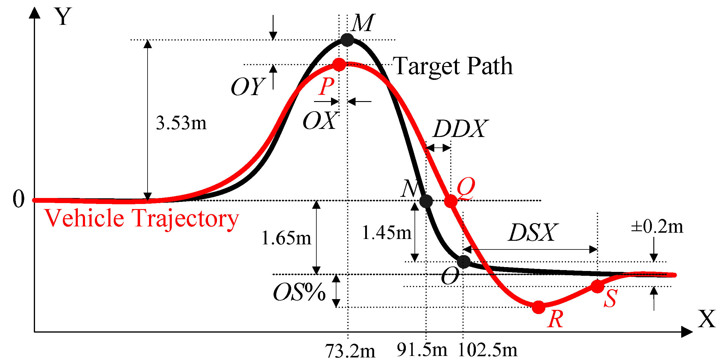
Figure 3 shows both the vehicle’s trajectory and the target path. In this paper, five measures, representing path-tracking performance, were defined, as in (20), based on the points along the target path and the vehicle’s trajectory: the peak’s center offset, OX, the peak’s lateral offset, OY, the percentage overshoot, OS%, the response delay, DDX, and the settling delay, DSX. These measures are depicted in Figure 3. In (20), X and Y in the parentheses correspond to the x- and y-positions of the points, M, N, O, P, Q, R, and S, respectively. In essence, smaller absolute values of these measures corresponded to improved path-tracking performance:

$$\left\{\begin{array}{l}OX=P\left(X\right)-M\left(X\right)=P\left(X\right)-73.20\\ OY=P\left(Y\right)-M\left(Y\right)=P\left(Y\right)-3.53\\ DDX=Q\left(X\right)-N\left(X\right)=Q\left(X\right)-91.50\\ DSX=S\left(X\right)-O\left(X\right)=S\left(X\right)-102.50\\ OS\%={\displaystyle \frac{\left|R\left(Y\right)\right|-1.65}{1.65+3.53}}\times 100\end{array}\right.$$

(20)

In Figure 3, OX and OY represent the agility and reachability of the path-tracking controller, respectively. In this study, if OY exceeded −0.05 m, the path-tracking performance was regarded as satisfactory. In this paper, the LQR was tuned such that OY was near −0.02 m. OS% implies lateral damping, which reflects agility. In this paper, if OS% remained less than 16% = 0.85 m, it was considered that the performance was satisfactory. DDX corresponds to response delays, signifying the agility of longitudinal motion. This measure is exactly proportional to μ. DSX can be interpreted as settling time, indicating the convergence speed of the vehicle’s lateral motion toward a target y-position, i.e., −1.65 m. In this paper, if DSX was less than 16 m, it was considered that the performance was satisfactory. Generally, the best performance was attained when OS% was near 1%, provided that ΔY was larger than −0.05 m. More comprehensive explanations of these metrics can be found in [16,17,43].

It is natural that OX and DDX increase as μ decreases. In other words, these variables are hard to reduce using the LQR. If k_v increases for a longer preview distance, then OX and OY decrease. For this reason, it is necessary to tune k_v and the weights in the LQ objective function simultaneously. From this idea, the APDS was proposed.

4. Simulation and Discussion

A simulation was performed to verify the path-tracking performance of the proposed APDS in terms of the five measures presented in (20). The LQRs, i.e., K_FWS and K_4WS, were implemented and designed on MATLAB/Simulink 2019a, connected with CarSim [48]. A target path in Figure 3 was selected as a test scenario. In the simulation, the F-segment sedan model provided in CarSim was selected [48]. From the model, the parameters of the bicycle model can be found in [16,17]. The steering actuators of FWS and 4WS were modeled as the 1st-order system, where the time constant was 0.05. When designing the LQRs, the speed controller in CarSim was applied in order to keep the constant speed, 60 km/h.

4.1. First Step: Design of LQR for Several μ Conditions

In this section, LQRs with FWS and 4WS were designed for each μ, divided from 0.3 to 0.8 at intervals of 0.1. This was achieved by tuning k_v and the weights, ξ_i, in J_FWS and J_4WS for different μ values.

Table 1. Summary of the tuning results of the LQR for FWS.

μ	kv	OX	OY	OS%	DDX	DSX
0.3	0.354	4.00	−0.020	0.0	15.11	14.35
0.4	0.229	1.47	−0.021	0.3	7.70	4.12
0.5	0.212	0.97	−0.020	0.8	3.87	−0.98
0.6	0.201	0.72	−0.020	0.6	2.35	−1.46
0.7	0.196	0.61	−0.019	0.7	1.54	−2.59
0.8	0.194	0.56	−0.020	0.7	1.24	−2.70

and

Table 2. Summary of the tuning results of the LQR for 4WS.

μ	kv	OX	OY	OS%	DDX	DSX
0.3	0.372	4.00	−0.020	0.0	15.11	14.35
0.4	0.242	1.67	−0.020	0.5	7.88	4.29
0.5	0.213	1.02	−0.020	0.5	3.94	0.01
0.6	0.203	0.77	−0.021	0.6	2.41	−1.32
0.7	0.198	0.61	−0.019	0.7	1.54	−2.59
0.8	0.195	0.62	−0.020	0.8	1.30	−2.73

show the tuning results of LQRs with FWS and 4WS for each μ. The values of the five measures on the same μ condition, as shown in Table 1 and Table 2, were nearly identical to one another. This means that FWS and 4WS can yield identical results, and that 4WS is not needed for path tracking.

Table 3. Summary of the simulation results of K_FWS (0.8).

μ	kv	OX	OY	OS%	DDX	DSX
0.3	0.194	10.34	0.633	5.8	23.95	42.42
0.4	0.194	4.03	0.208	1.8	11.04	10.20
0.5	0.194	1.28	0.020	1.9	4.19	2.60
0.6	0.194	0.76	−0.007	0.7	2.36	1.25
0.7	0.194	0.63	−0.016	0.7	1.54	0.42
0.8	0.194	0.56	−0.020	0.7	1.24	0.27

and

Table 4. Summary of the simulation results of K_4WS (0.8).

μ	kv	OX	OY	OS%	DDX	DSX
0.3	0.195	10.22	0.612	3.9	23.93	36.07
0.4	0.195	4.05	0.205	1.1	11.11	10.75
0.5	0.195	1.31	0.020	1.3	4.27	2.97
0.6	0.195	0.80	−0.007	0.7	2.42	1.35
0.7	0.195	0.66	−0.015	0.8	1.59	0.49
0.8	0.195	0.62	−0.020	0.8	1.30	0.32

show the simulation results of K_FWS (0.8) and K_4WS (0.8) with the corresponding k_v values. As shown in Table 3 and Table 4, the path-tracking performance was deteriorated because μ was not considered. Especially, the performance deterioration was severe at low conditions, such as 0.3 and 0.4.

As shown in Table 1 and Table 2, the velocity gain, k_v, became larger as μ decreased. In other words, a larger k_v is needed in low μ conditions. These results imply that the preview distance, L_p or k_v, should be adjusted according to the variations in μ. From Table 1 and Table 2, K_FWS (0.8) and K_4WS (0.8) were obtained. We denoted the first step as CASE1.

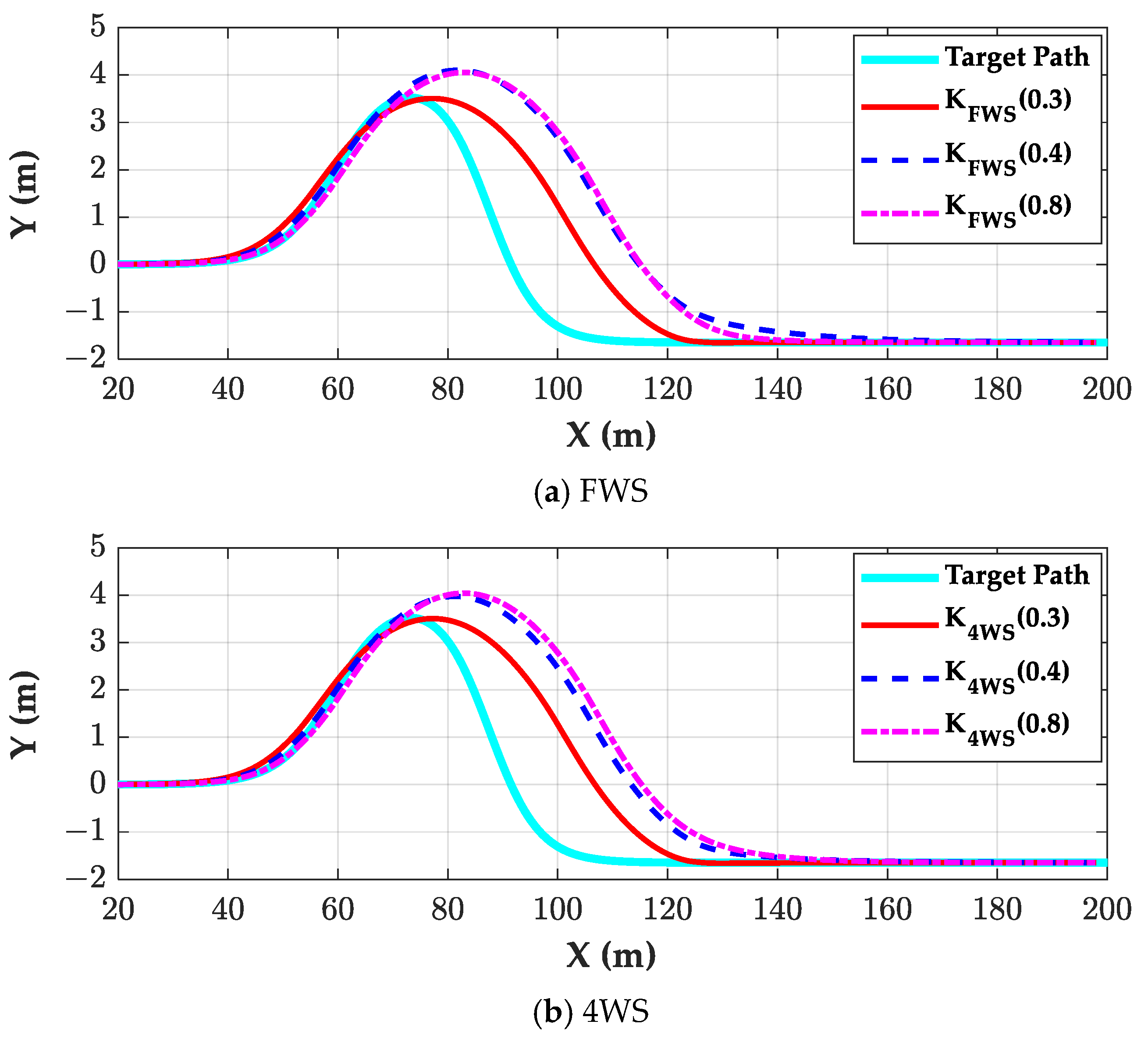
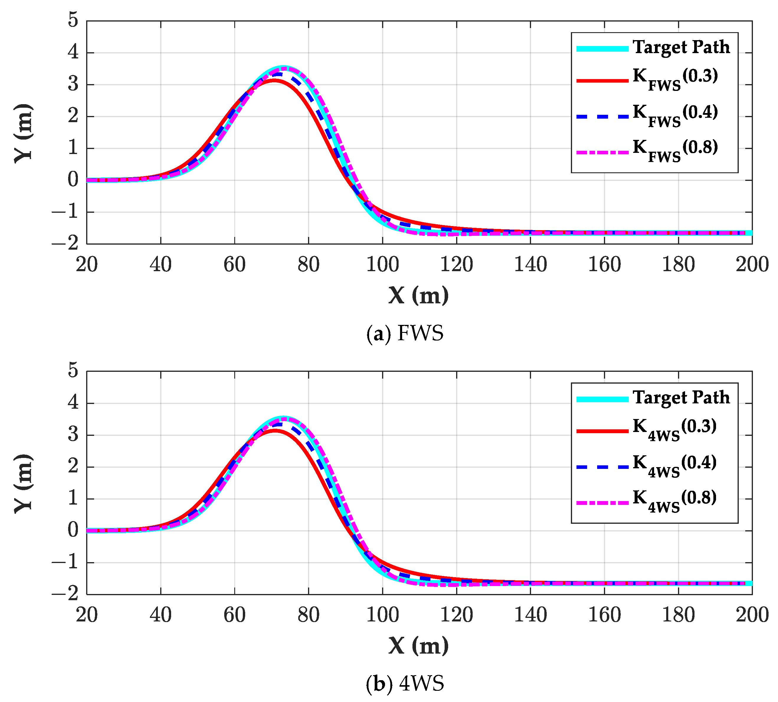
Figure 4 and Figure 5 show the simulation results of K_FWS (0.8) and K_4WS (0.8) on the road where μ was 0.3 and 0.8, respectively. In Figure 4, K_FWS (0.3) and K_4WS (0.3) were the best controllers for FWS and 4WS, respectively. Similarly, in Figure 5, K_FWS (0.8) and K_4WS (0.8) were the best controllers for FWS and 4WS, respectively.

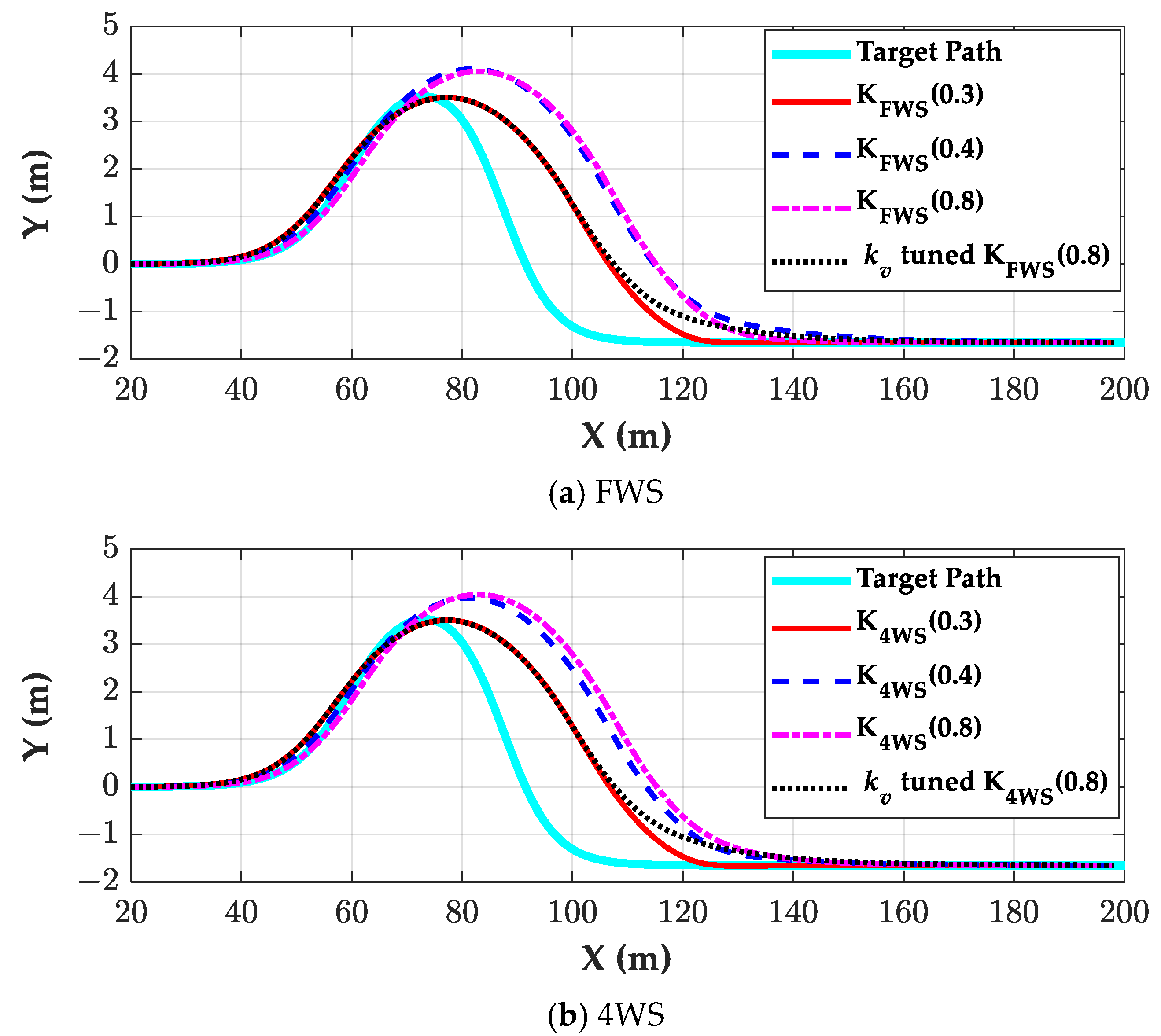
As shown in Figure 4, those controllers tuned on the road where μ was 0.4 or 0.8 showed poor path-tracking performance because they were not designed on the road where μ was 0.3. The controllers, K_FWS (0.4), K_4WS (0.4), K_FWS (0.8), and K_4WS (0.8), showed large overshoot along the positive lateral direction. On the other hand, as shown in Figure 5, those controllers tuned on the road where μ was 0.3 or 0.4 showed poor path-tracking performance on the road where μ was 0.8 because the preview distances of these controllers were too large. As a result, there were large negative OY values, which can cause collision. Generally, a controller designed under low μ conditions has a larger preview distance than those designed under high μ conditions.

For better performance, the preview distance, L_p, or the velocity gain, k_v, should be tuned with the fixed gains, K_FWS (0.8) and K_4WS (0.8), according to the variations in μ. This was performed in the second step.

4.2. Second Step: Tuning of k_v Under Different μ Conditions with Fixed LQR Gains

In this section, the velocity gain, k_v, was tuned with the fixed LQR gains, i.e., K_FWS (0.8) and K_4WS (0.8), under different μ conditions. It should be noted that only k_v was tuned for the best path-tracking performance.

Table 5. Summary of the tuning results of k_v for FWS.

μ	kv	OX	OY	OS%	DDX	DSX
0.3	0.388	4.05	−0.020	0.0	15.99	32.29
0.4	0.272	1.99	−0.021	0.0	8.35	10.16
0.5	0.211	0.95	−0.019	0.8	3.83	2.87
0.6	0.200	0.67	−0.019	0.5	2.27	1.47
0.7	0.196	0.60	−0.019	0.7	1.51	0.47
0.8	0.194	0.56	−0.020	0.7	1.24	−2.70

and

Table 6. Summary of the tuning results of k_v for 4WS.

μ	kv	OX	OY	OS%	DDX	DSX
0.3	0.390	4.05	−0.019	0.0	16.14	33.55
0.4	0.273	2.01	−0.021	0.0	8.42	11.01
0.5	0.213	0.97	−0.020	0.5	3.90	3.29
0.6	0.201	0.72	−0.019	0.6	2.34	1.47
0.7	0.197	0.65	−0.019	0.8	1.57	0.52
0.8	0.195	0.62	−0.020	0.8	1.30	−2.73

show the tuning results of k_v for K_FWS (0.8) and K_4WS (0.8) under different μ conditions. As shown in the tables, with the fixed gains, tuning the single parameter k_v could provide comparable results to those in Table 1 and Table 2, and improved results from Table 3 and Table 4. More specifically, OX, OY, and DSX of K_FWS (0.8) on the road where μ was 0.3 were improved from 10.34, 0.633, and 42.42 to 4.05, −0.020, and 32.39, respectively. In terms of OX and DSX, through the tuning of k_v, those values were reduced by 60% and 24%, respectively. However, in the second step, DSX values were deteriorated on the road where μ was 0.3 or 0.4. This was inevitable because the lateral tire force was small under low μ conditions.

As mentioned earlier, this step did not need different gains under corresponding μ conditions. It needed only a single fixed gain, i.e., K_FWS (0.8) or K_4WS (0.8). We denoted the second step as CASE2.

Figure 6 shows the simulation results of the tuned k_v with K_FWS (0.8) and K_4WS (0.8) on the road where μ was 0.3. As shown in Figure 6, the tuned k_v values with K_FWS (0.8) and K_4WS (0.8) showed good path-tracking performance, compared to the tuning results in Table 1 and Table 2. However, there were large differences among the settling delays, DSX, in Table 1 and Table 5, and Table 2 and Table 6. On the contrary, the values of OX and OY in Table 1 and Table 5, and Table 2 and Table 6 were nearly identical to one another. This indicates that collision avoidance was satisfied with the tuned k_v with K_FWS (0.8) and K_4WS (0.8), regardless of the magnitude of DSX.

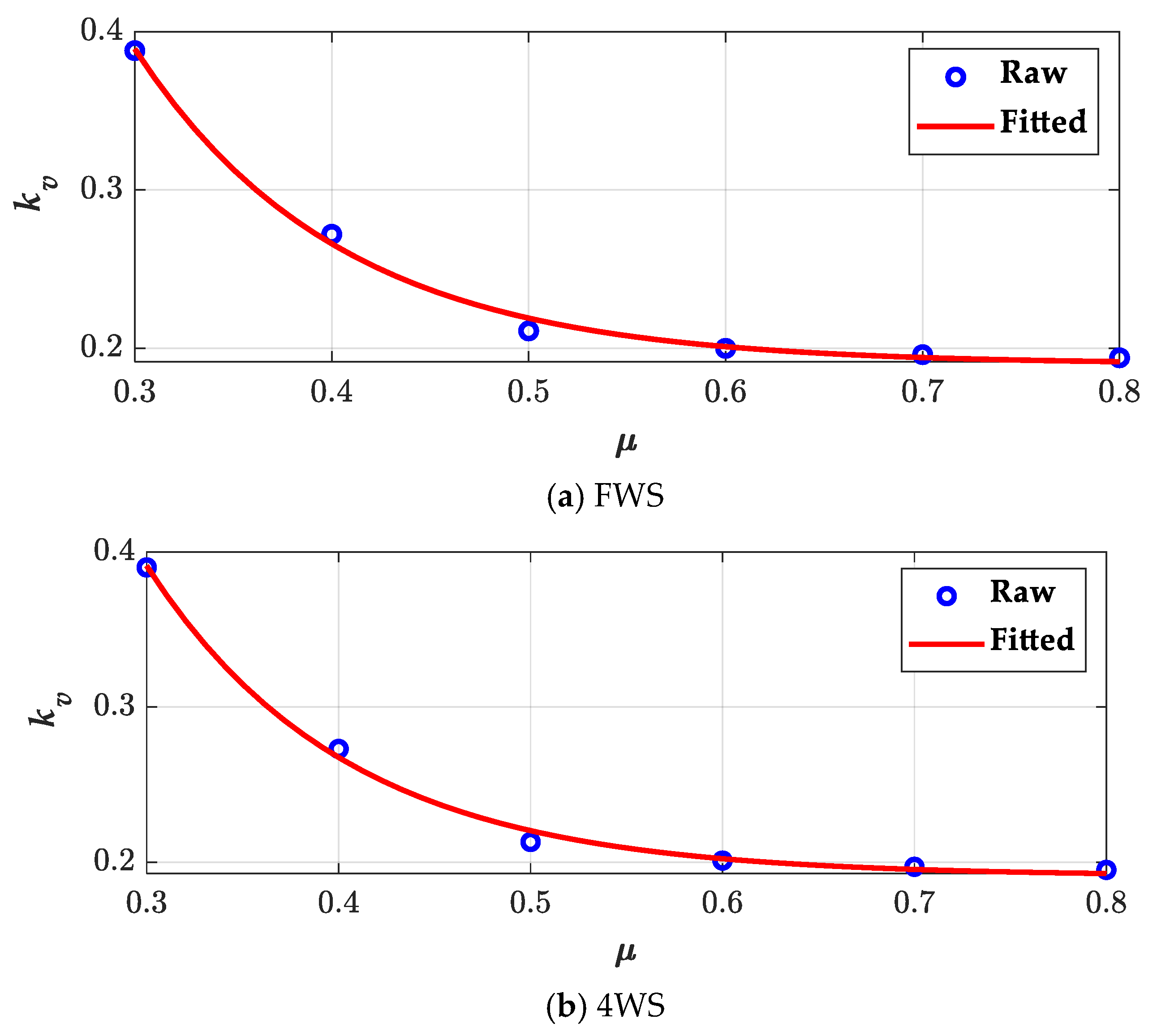
4.3. Third Step: Curve Fitting with the Velocity Gain, k_v, with Respect to μ

In this section, curve fitting was applied to the tuned k_v values in Table 5 and Table 6 for K_FWS (0.8) and K_4WS (0.8) with respect to μ. For curve fitting, the exponential function in (19) was adopted. Figure 7 shows the curve-fitting results of k_v with respect to μ for FWS and 4WS. As shown in Figure 7, the velocity gains were well fitted with the exponential function, and there were little differences between FWS and 4WS.

To validate the curve fitting of k_v over μ, a simulation was performed using the exponentially fitted k_v with K_FWS (0.8) and K_4WS (0.8) under different μ conditions. To emphasize the estimation performance of the curve fitting, μ was divided from 0.3 to 0.8 at intervals of 0.05.

Table 7. Summary of the curve-fitting results of k_v for FWS.

μ	OX	OY	OS%	DDX	DSX
0.30	4.00	−0.025	−0.1	15.92	32.29
0.35	3.13	0.014	0.0	12.07	20.45
0.40	2.14	−0.005	0.0	8.55	10.05
0.45	1.27	−0.032	1.1	5.50	4.50
0.50	0.78	−0.037	0.4	3.67	3.05
0.55	0.68	−0.029	0.2	2.88	2.48
0.60	0.65	−0.022	0.5	2.27	1.44
0.65	0.63	−0.018	0.7	1.79	0.76
0.70	0.61	−0.016	0.7	1.54	0.43
0.75	0.61	−0.016	0.8	1.37	0.28
0.80	0.60	−0.015	0.8	1.27	0.20

and

Table 8. Summary of the curve-fitting results of k_v for 4WS.

μ	OX	OY	OS%	DDX	DSX
0.30	4.00	−0.024	−0.1	16.06	33.55
0.35	3.11	0.013	0.0	12.15	22.14
0.40	2.16	−0.007	0.0	8.60	10.89
0.45	1.30	−0.032	0.6	5.57	4.97
0.50	083.	−0.037	0.2	3.76	3.52
0.55	0.72	−0.029	0.2	2.93	2.64
0.60	0.68	−0.022	0.5	2.30	1.52
0.65	0.68	−0.018	0.7	1.84	0.83
0.70	0.66	−0.016	0.8	1.59	0.50
0.75	0.65	−0.015	0.8	1.42	0.33
0.8	0.63	−0.015	0.8	1.32	0.25

show the simulation results of the exponentially fitted k_v for FWS and 4WS. As shown in the tables, the performance of the APDS was comparable to the results in Table 5 and Table 6. We denoted the third step as CASE3.

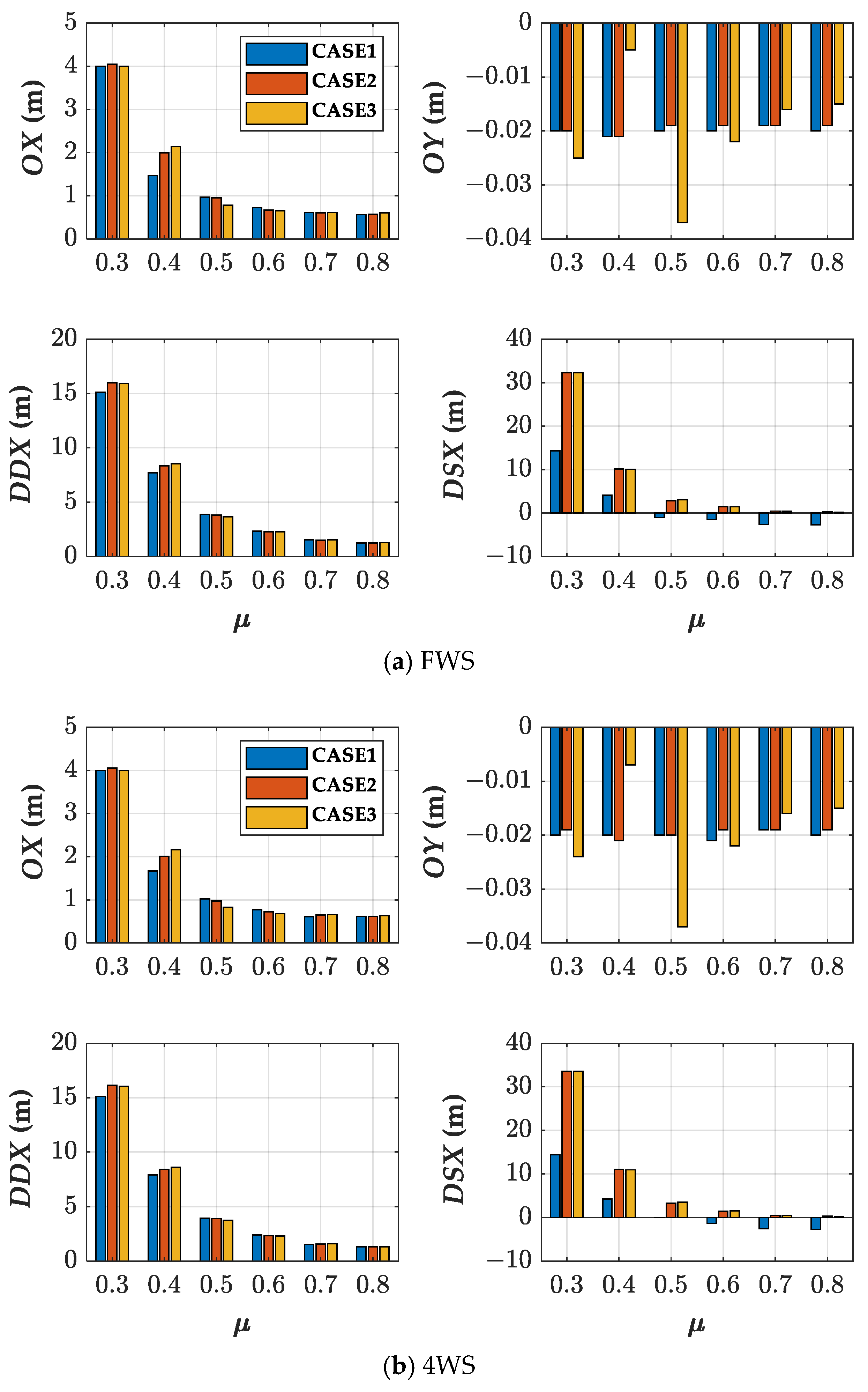
Figure 8 shows the comparison results among the three cases, CASE1, CASE2, and CASE3, for FWS and 4WS. As shown in Figure 8, there were small differences among OX, OY, and DDX for different μ conditions. However, there were large differences among DSX on the road where μ was 0.3 and 0.4. These results mean that the proposed APDS was effective for different μ conditions.

Figure 8 shows that there were little differences between FWS and 4WS. This indicates that additional actuators, such as 4WIB and 4WID, had little influence on the performance of the APDS.

5. Conclusions

The aim of this study was to design a path-tracking controller that was robust against the variations in tire–road friction for autonomous vehicles. To cope with tire–road friction variation, the APDS was proposed. The state-space model was derived from a target path and a 2-DOF bicycle model. With the state-space model, the LQR was selected as a controller design methodology. FWS and 4WS were selected as actuators for path tracking. In the APDS, the tuned velocity gains for several tire–road friction coefficients were exponentially fitted with respect to tire–road friction. To show the proposed adaptive preview distance scheme, a simulation study was performed on the vehicle simulation package, CarSim. From the simulation results, the following conclusions were drawn:

• The proposed adaptive preview distance scheme was effective under several tire–road friction conditions in terms of several measures defined for path tracking. Especially, every measure obtained from the adaptive preview distance scheme was comparable to those of the finely tuned LQR, except the settling delay, DSX. Moreover, DSX was deteriorated only under low tire–road friction conditions.
• The proposed adaptive preview distance scheme was quite simple to design and apply. It used a fixed gain, which was designed under high tire–road friction conditions. Only the velocity gain should be tuned for several tire–road friction conditions. The curve fitting with the exponential function was also easy and simple to apply.
• FWS and 4WS, used as steering actuators, had little differences between them in terms of the path-tracking performance. This fact indicates that additional actuators, such as 4WIB and 4WID, would have little effect on the path-tracking performance of the adaptive preview distance scheme.

The limitation of this study is that this method did not consider the variation in the vehicle speed. Especially, high-speed conditions have large effects on the path-tracking performance. In future research, the vehicle speed will be selected as a time-varying parameter.