Thermal Error Transfer Prediction Modeling of Machine Tool Spindle with Self-Attention Mechanism-Based Feature Fusion

Abstract

Thermal errors affect machining accuracy in high-speed precision machining. The variability of machine tool operating conditions poses a challenge to the modeling of thermal errors. In this paper, a thermal error model based on transfer temperature feature fusion is proposed. Firstly, the temperature information fusion features are built as inputs to the model, which is based on a self-attention mechanism to assign weights to the temperature information and fuse the features. Secondly, an improved direct normalization-based adaptive matrix approach is proposed, updating the background matrix using an autoencoder and reconstructing the adaptive matrix to realize domain self-adaptation. In addition, for the improved adaptive matrix, a criterion for determining whether the working conditions are transferrable to each other is proposed. The proposed method shows high prediction accuracy while ensuring training efficiency. Finally, thermal error experiments are performed on a VCM850 CNC machine tool.

1. Introduction

With the demand for high-speed and high-precision machine tools increasing dramatically, thermal errors caused by thermal deformation are one of the factors affecting machining accuracy, accounting for 40–70% of the total errors affecting machining accuracy [1]. Thermal error modeling and compensation is one of the most effective methods to improve machining accuracy [2]. The research scope of this paper is the thermal error of spindles caused by temperature.

Research on methods to reduce and eliminate thermal errors has always been a hot topic [3]. The error compensation method can create an artificial error to eliminate or reduce the original thermal error, which has the advantages of a wide range of applications and low cost [4,5]. Thermal error modeling methods are mainly divided into two types: mechanism models and data-driven models [6]. A common data-driven method is based on establishing the mapping relationship between the surface temperature and spindle thermal error using a learning mechanism, which does not rely on much a priori knowledge but on easy-to-collect sensor data [7]. There are various models for predicting the thermal error of machine tools, such as multiple regression, neural networks, time series, gray theory, etc. [8,9]. Wu et al. proposed a thermal image-based modeling method for the radial thermal error of CNC machine tool spindles, using the features of a convolutional neural network as a deep neural network that automatically extracts the features of the input data to further improve the accuracy of the spindle radial thermal error prediction model [10]. Yu et al. proposed a thermal error model based on LSTM, which can judge the interval of real-time speed in the thermal error prediction process and select the corresponding model to improve prediction accuracy [11]. However, the above methods are all assumed to have the same probability distribution for the training and test data [12]. This leads to two unavoidable problems: First, the model generalization is poor. Zhu et al. proposed a thermal error modeling method based on random forest, which has better prediction performance under the same operating conditions but larger prediction errors under other operating conditions [13]. Second, the training set requirement is large; the success of the model depends on sufficient labeled data to train the machine learning mode [14,15]. Zhang et al. proposed a thermal error prediction model based on a convolution neural network, and the generalization was improved using four operating conditions for the training set [16]. However, obtaining a large amount of labeled data is usually expensive and time-consuming [17]. In fact, the practical application is faced with model prediction under different working conditions, and usually, the probability distributions of training data and test data are not consistent [18]. The existing methods are difficult to deal with in terms of problems across domains, which is the main reason for the unsatisfactory results of the related research. Transfer learning adjusts the probability distributions of training and test data, which is a way to improve the predictive power of thermal error models. Compared with the time-consuming training of deep learning, migration learning can accomplish the prediction model quickly.

Transfer learning does not require the source and target domains to be sampled from the same probability distribution. It only requires that they come from related tasks, which improves the robustness of the model [19]. Transfer learning transfers the knowledge contained in the training dataset to the test dataset, improving the generalization ability of the model [20]. Existing transfer learning methods can be categorized into two kinds: one is by adjusting weights, and the other is by feature transfer, also known as subspace learning and neighborhood adaptation [21,22]. Many scholars have researched the method of adjusting weights. Liu et al. first proposed an error control method based on transfer learning using a fine-tuning method for transfer learning to enhance robustness and generalization ability [23]. Kuo et al. combined transfer learning with model optimization in order to improve prediction accuracy and avoid wasting time with repeated training [24]. These studies show that transfer learning allows deep learning methods to be adapted to datasets acquired from machines under different operating conditions [25]. However, these methods can only be fine-tuned using networks that have been pre-trained. There is no mutual transfer or transformation of data features from source and target domains to a unified feature space through feature changes to narrow the gap between source and target domains [26]. Adjusting the probability distributions of training and test data through feature transfer is another way to improve the predictive power of thermal error models.

To realize the thermal error prediction across operating conditions, an SA-DS-EasyTL model is proposed to improve the prediction capability of a spindle thermal error prediction model using feature transfer. Thermal error experiments, temperature fields, and thermal error measurements were performed on a VMC850 CNC machining center. The available information between different datasets in the transfer learning model was utilized. The model’s self-attention mechanism selected important temperature information to avoid coupling between the temperature variables, leading to the degradation of model training accuracy. The feature fusion of important temperature information by attention weights improved the model performance. Using direct standardization, the target domain was corrected to match the source domain. In transfer learning EasyTL, the source and target domain datasets were projected into the transfer subspace to enhance the distribution alignment similarity of the two domains. The domain adaptive module included a domain classifier and a domain distribution difference metric term to make the learned features domain invariant.

The subsequent organization of this paper is as follows: in Section 2, the concepts of experimental data collection and transfer learning are introduced. In Section 3, the SA-DS-EasyTL model for thermal error prediction is developed. The components and principles of the model are presented. In Section 4, the validation of the transfer model is analyzed. In Section 5, the performance of the thermal error modeling is analyzed under different working conditions. In Section 6, the conclusion is summarized.

2. Experimental Data of Spindle Thermal Errors

The thermal error experiments in this section were carried out on a VMC850 CNC machine tool in Chengdu, China. The machine tool temperature and spindle thermal error data at different speeds of the spindle were obtained by the five-point method [27]. In this experiment, the spindle thermal errors were measured using five Lion Precision capacitive displacement sensors, while 30 PT100 platinum resistance temperature sensors were used to capture the machine tool’s temperature field. The measuring equipment, the installation position of the displacement sensors, and the location of the temperature sensors are shown in Figure 1. The training data and test data were randomly selected from different operating conditions.

The test time was 4 h for each speed. The temperature and thermal error data were collected every 5 s. The spindle thermal error measurement data of the Z-direction were used in subsequent calculations and verifications. Five experimental datasets were collected, including one 2000 rpm, one 4000 rpm, one 4000 rpm with the machine tool uncooled, and two variable speeds. Partial temperature sensors, spindle Z-direction thermal error data, and spindle speed plots for the two variable speeds are shown in Figure 2 and Figure 3. Figure 2a shows the temperature data of 10 of the 30 temperature measurement points at variable speed 1 with the spindle speed as the background, and Figure 2b shows the spindle axial thermal error data with the spindle speed as the background. It can be seen from Figure 3 that the trend of temperature and thermal error is related to the spindle speed.

3. SA-DS-EasyTL Error Prediction Model

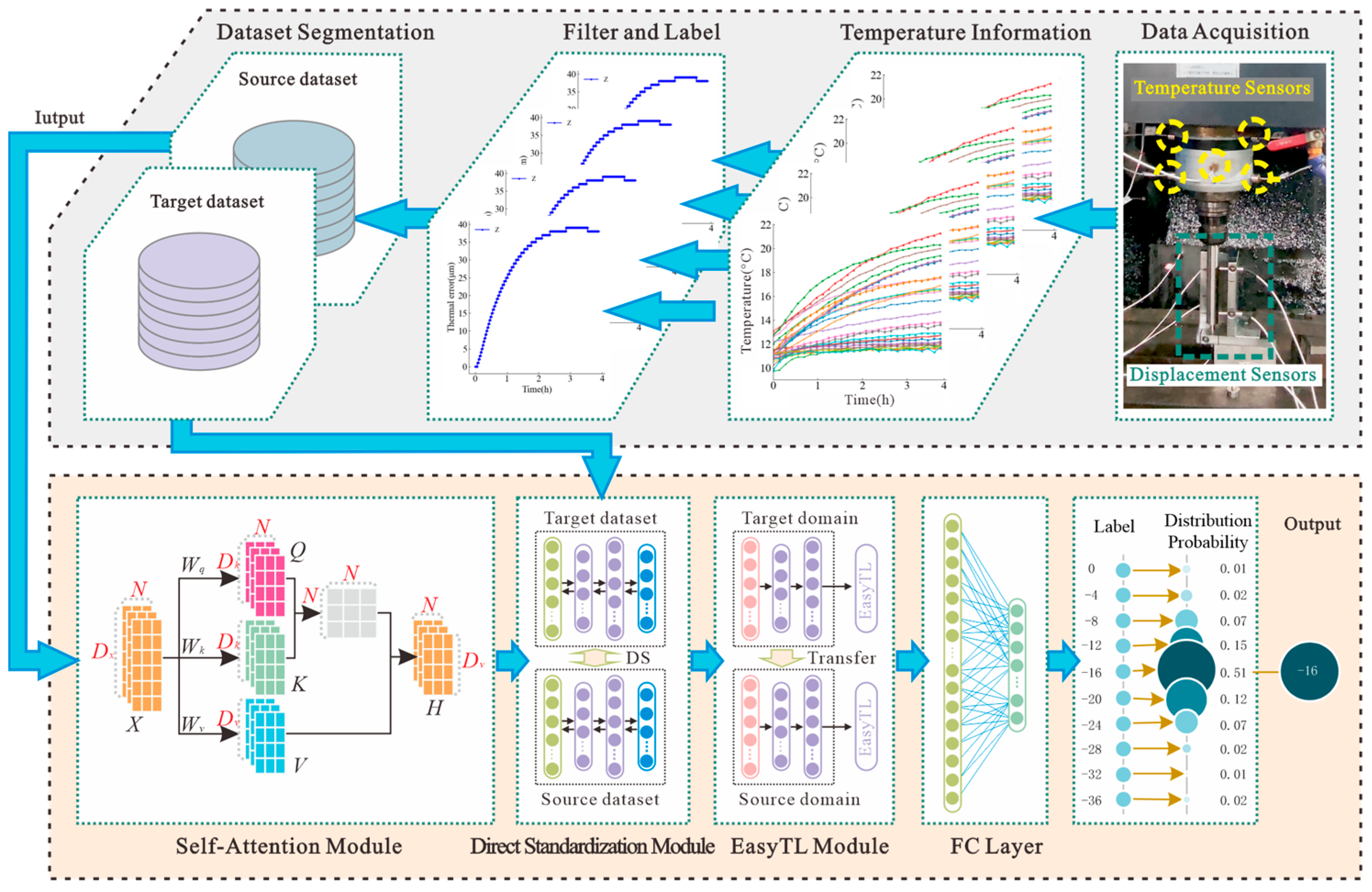
In this paper, an SA-DS-EasyTL-based thermal error prediction model is established. The temperature feature fusion is efficiently accomplished in two steps: first, extract the influential temperatures; second, fuse the influential temperatures. Direct standardization spatially corrects the fused target domain X_t to match the source domain X_s. The EasyTL algorithm aligns the source domain X_s and the target domain X_t in-domain and then learns the nonparametric transfer model of the target domain X_t through in-domain programming. The flowchart of the proposed model is shown in Figure 4.

3.1. Temperature Feature Fusion

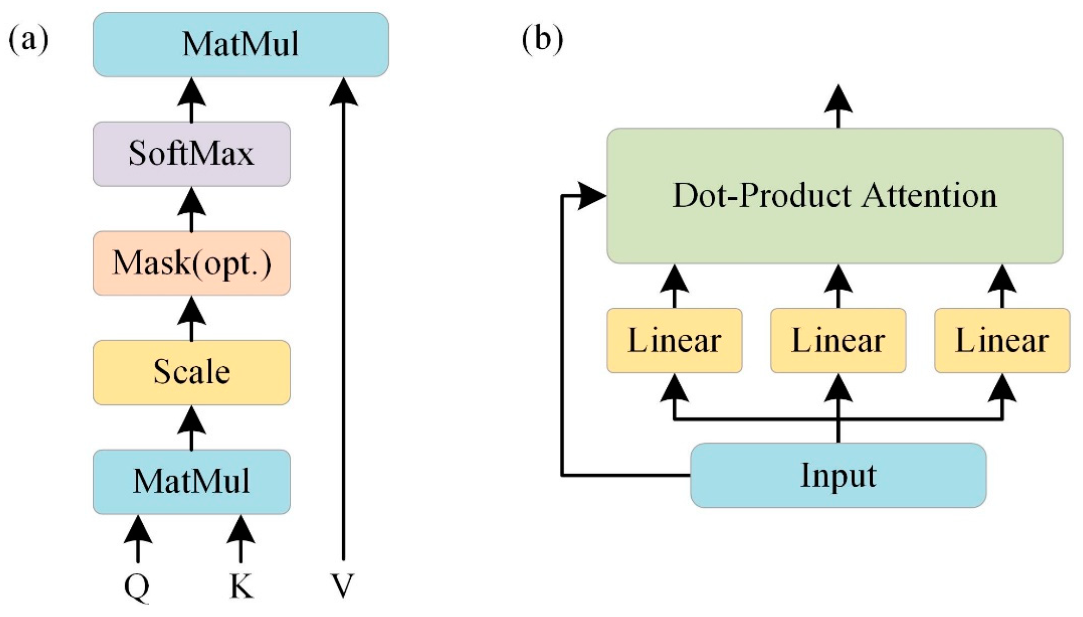
The self-attentive mechanism is a variant of the attention mechanism that is less dependent on external information and more adept at capturing the internal relevance of data or features [28]. The core of self-attention mechanism is dot-product attention. The calculation process of dot-product attention is shown in Figure 5, which is defined as follows:

$$Attention(Q, K, V) =softmax({\displaystyle \frac{Q{K}^{\mathrm{T}}}{\sqrt{d_k}}})V$$

(1)

where Q, K, and V denote “query”, “key”, and “value”, respectively, and d_k is the scaling factor, which represents the dimension of K. For the larger d_k value, the product of the dot product is too large, so the softmax function is pushed to the region with a minimal gradient. To counteract this effect, $\frac{1}{\sqrt{d_k}}$ is used to scale point the product.

Too many temperature variables increase the experimental cost and workload, and the coupling phenomenon between temperature variables also affects the modeling accuracy. Meanwhile, too few temperature variables weaken the robustness of the model and reduce the prediction performance due to the lack of key information that causes thermal errors. Therefore, establishing efficient temperature feature fusion is a critical step before thermal error modeling. Figure 6 shows the temperature feature fusion framework.

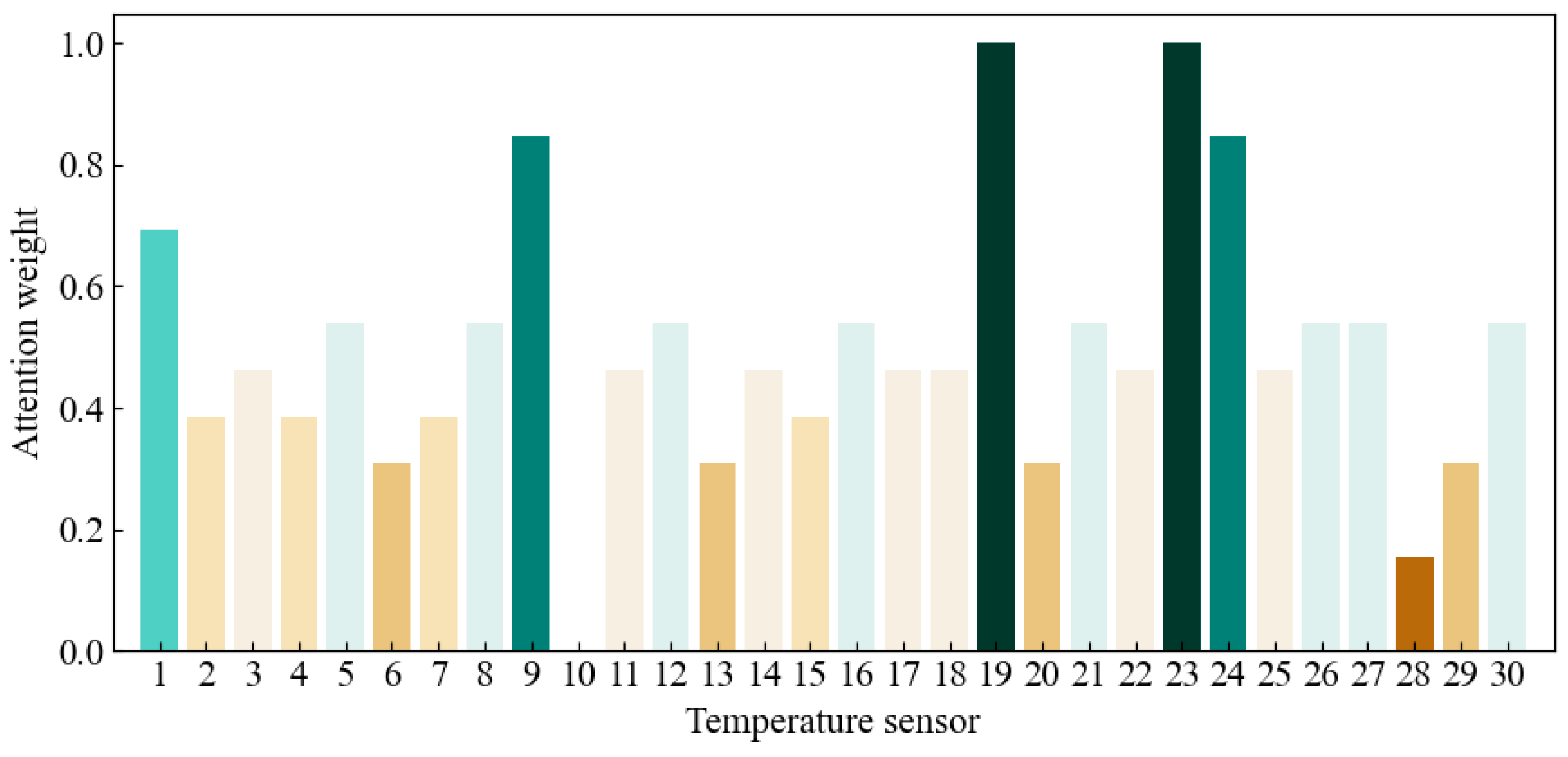
The attention weights of the temperature-sensitive points of the machine tool selected based on the self-attention mechanism are shown in Figure 7. An attention weight close to 0 means that the temperature sensor has no importance, while an attention weight close to 1 means that the temperature sensor has high importance. Sensor 19 and Sensor 23 have the highest attentional weight, which can reach 1. This is followed by Sensor 9 and Sensor 24, with an attentional weight of 0.846. The lowest attentional weight is Sensor 10, which is only 0.

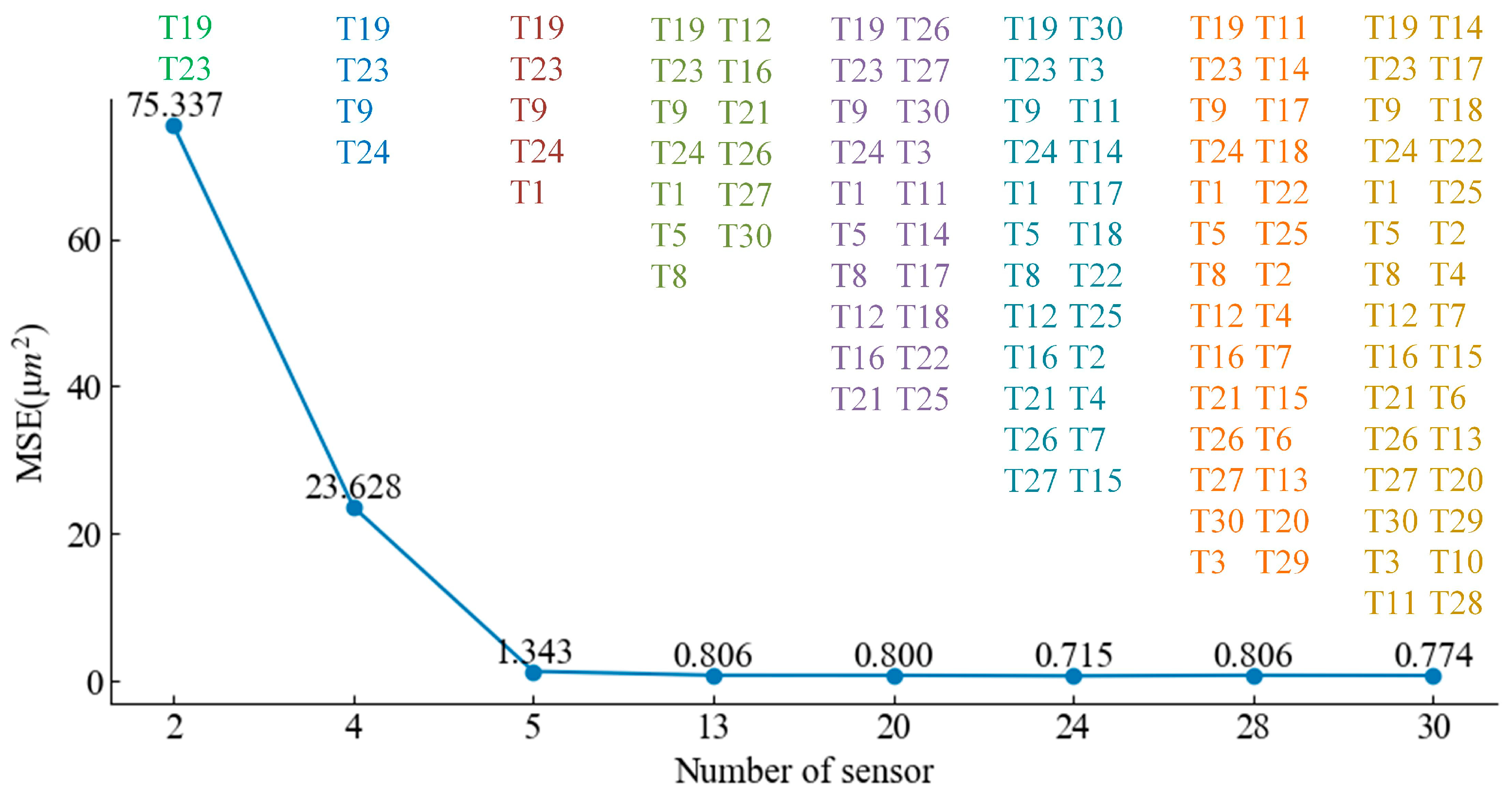
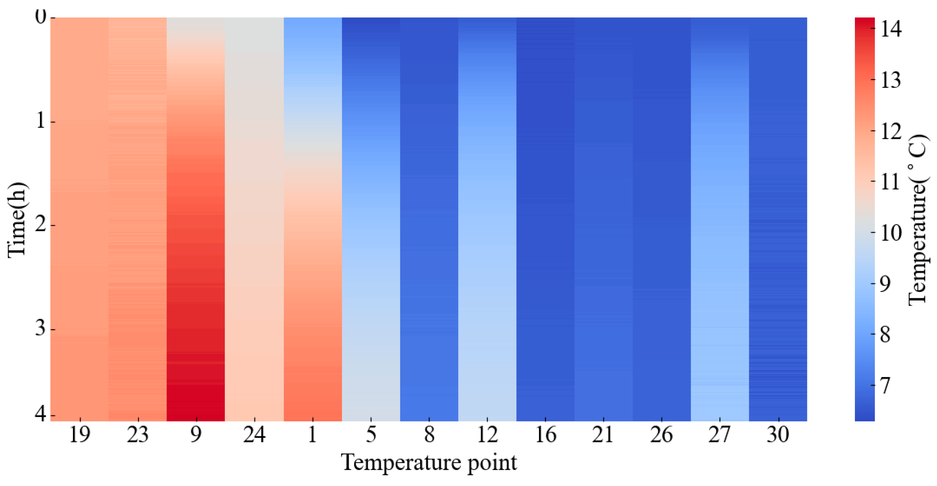
Even if temperature features with low attentional weights are eliminated, these temperature features still have redundancy and create problems in the high dimensional space. It is necessary to fuse multiple features into new feature data using attentional weights. The EasyTL model was used to train the prediction for 2000 rpm with mean squared error (MSE) as the evaluation metric. The least important features were iteratively eliminated based on the ranking of the feature attention weight. As can be seen in Figure 8, with the elimination of redundant features and measurement noise, the accuracy is about 0.8 until only 13 features remain. Then, the prediction accuracy decreases as important features are eliminated, resulting in the loss of useful information, and the MSE even reaches 75.34 µm² at 2 features. By comparing the prediction accuracies of the model, a combination of 13 temperature feature fusions, i.e., T1, T5, T8, T9, T12, T16, T19, T21, T23, T24, T26, T27, and T30, were finally selected. The results of feature fusion are shown in Figure 9. The results show that this method helps to identify and eliminate redundant features and improves the performance of the model.

3.2. Spatial Correction with Direct Standardization

The DS method corrects the space of the target domain to match the space of the source domain while keeping the source domain unchanged [29]. At present, direct standardization (DS) algorithms are used more often in model transfer and achieve good results. The temperature feature matrices in the source and target domains are correlated. The source and target domain matrices after feature fusion are set to be X_s(m × p) and X_t(m × p), where m is the number of features, and p is the length of each feature, assuming that

$$X_t=X_{s}F+1b_s^{\mathrm{T}}$$

(2)

where F(p × p) is the transformation matrix, and b_s(p×1) is the background correction matrix. A centering matrix C_m(m × m) is introduced

$$C_m=I_m-{\displaystyle \frac{1}{m}}{11}^{\mathrm{T}}$$

(3)

where I_m is a unit matrix of order m, and 1(m × 1) is a column vector with 1 in each element. Since 1b_s^T is the same per row vector, C_m1b_s^T = 0. Thus, multiplying both sides of Equation (3) simultaneously by the matrix C_m yields:

$$X_t=X_{s}F$$

(4)

$$F=(X_t^{\mathrm{T}}{X}_s{)}^{-1}{X}_t^{\mathrm{T}}{X}_t$$

(5)

The background correction matrix bs is obtained by multiplying both sides of Equation (2) simultaneously by (1/m)l^T:

$$b_{\mathrm{s}}=X_{1t}^{\mathrm{T}}-F^{\mathrm{T}}{X}_{1s}^{\mathrm{T}}$$

(6)

where both T_1m and T_1s are column vectors.

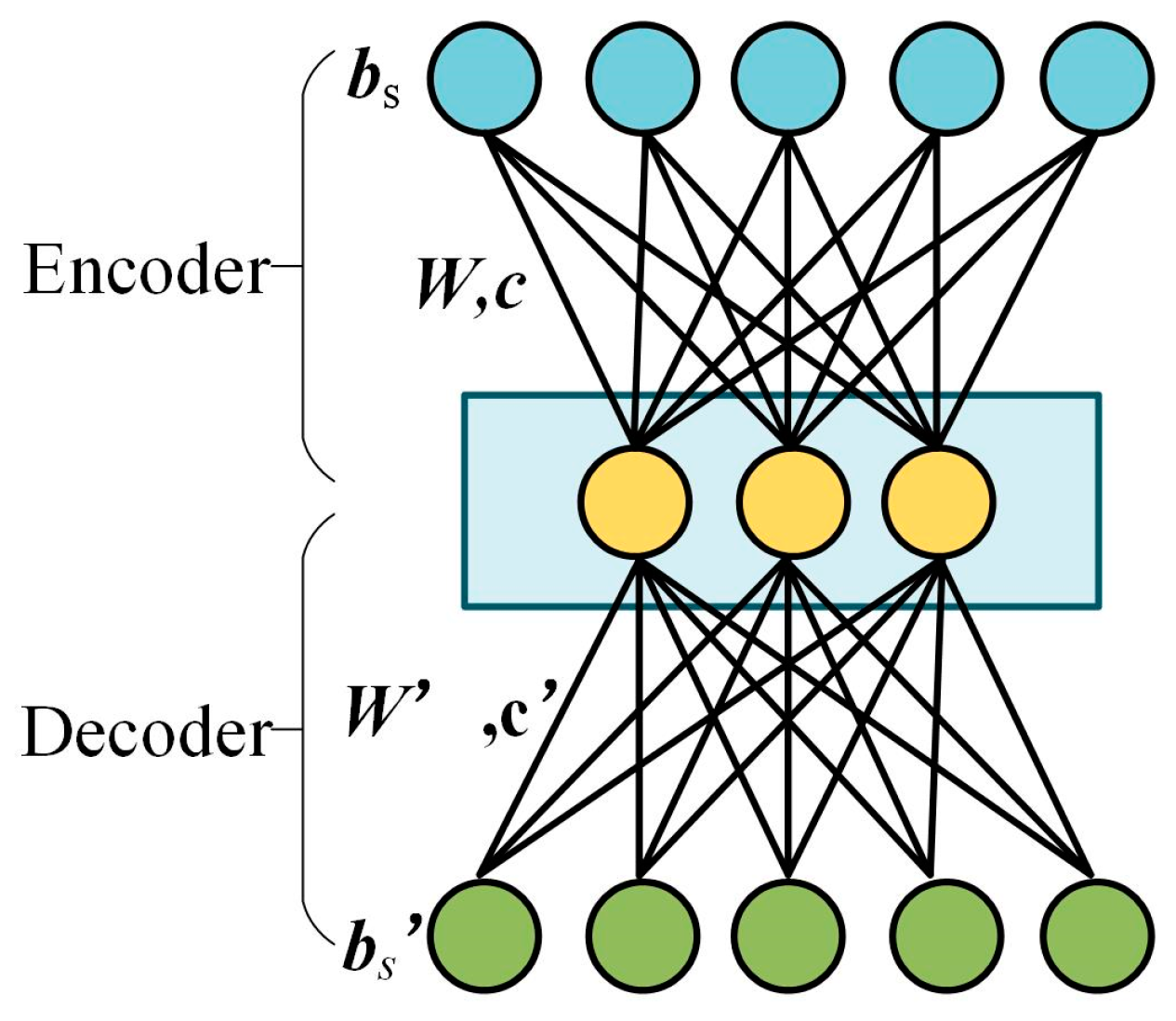
However, traditional direct normalization does not measure the spatial relationship between the source and target domains, and this study improves its structure to accommodate spatial features. b_s is adjusted through an autoencoder, a type of feed-forward neural network composed of an input layer, a bottleneck layer, and an output layer. The autoencoder’s structure and hyperparameters are designed with b_s serving as both the input and the reference output for the model. The encoder consists of an input layer and bottleneck layer. The decoder consists of a bottleneck layer and an output layer. The encoder maps the input vector x to the potential representation vector z through function f:

$$z=f(W{b}_{\mathrm{s}}+c)$$

(7)

where f is an activation function, W is a weight matrix, and c is a bias vector. The decoder maps the latent representation vector z to a reconstruction b_s′ by function g:

$$b_{\mathrm{s}}^{\prime }=g(z)=f^{\prime }(W^{\prime }z+c^{\prime })$$

(8)

where f′ is an activation function, W′ is a weight matrix, and b′ is a bias vector.

In the training process, W, b, W′, and b′ are optimized to minimize the average difference between the input vector b_s and the reconstruction vector b_s′. This difference is called reconstruction error. The loss function of the autoencoder is formulated by:

$$\mathrm{loss}(b_{\mathrm{s}}^{\prime },b_{\mathrm{s}})=\frac{1}{2}{\Vert b_{\mathrm{s}}^{\prime }-b_{\mathrm{s}}\Vert }^2$$

(9)

The structure and hyperparameters of the autoencoder are designed, and b_s is used as the input and reference output of the autoencoder model. After n times training, the autoencoder model and the reconstruction vector b_s′ are obtained (Figure 10).

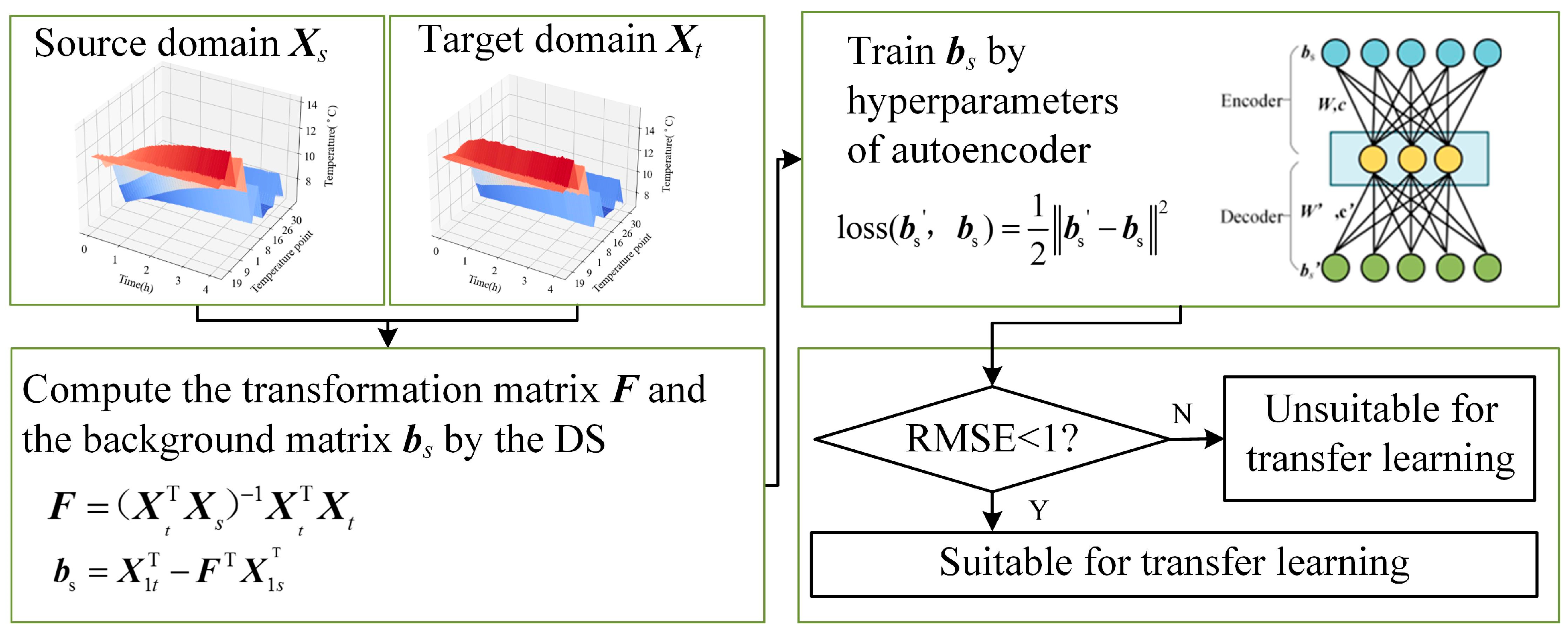
The RMSE is used to measure the appropriateness of transfer learning for the reconstruction vector b_s′. When the RMSE is less than 1, the spatial distance between the source and target domains is small and suitable for migration. When the RMSE is greater than 1, the spatial distance between the source and target domains is large and not suitable for migration. Figure 11 shows the framework of spatial correction.

3.3. Transfer Learning with EasyTL

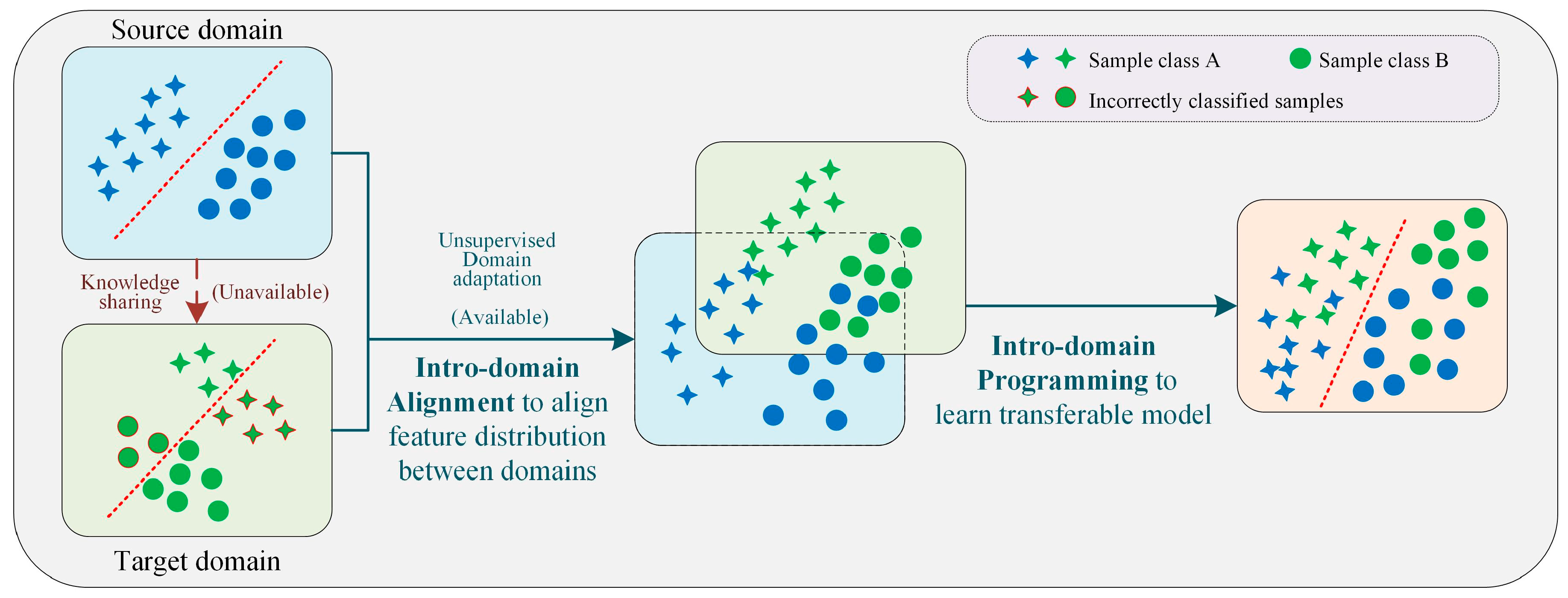
Transfer learning is a learning method that focuses on solving problems with only a few or even zero labeled samples in the target domain. Through transfer learning, the “knowledge” gained from historical tasks can be transferred to existing tasks to realize cross-domain knowledge application. EasyTL, the transfer learning used in this paper, has the advantages of nonparametric and efficient learning [30]. As shown in Figure 12, the EasyTL algorithm inputs the temperature matrix X_s after feature fusion in the source domain and the temperature matrix X_t after feature fusion in the target domain. X_s and X_t are then subjected to in-domain alignment, which aligns the different feature distributions in the source and target domains. An unsupervised domain adaptation method using correlation alignment (CORAL) is defined as follows:

$$X_s=X_s{\left(\mathrm{cov}(X_s)+E_s\right)}^{-\frac{1}{2}}{\left(\mathrm{cov}(X_t)+E_t\right)}^{-\frac{1}{2}}$$

(10)

where cov (−) is the covariance matrix; and E_s and E_t shape unit matrices equal to the source domain X_s and the target domain X_t, respectively. After feature transfer via intra-domain alignment, intra-domain programming learns a nonparametric transferable model of the target domain.

4. Validation of the Transfer Model

4.1. DS Correction Process

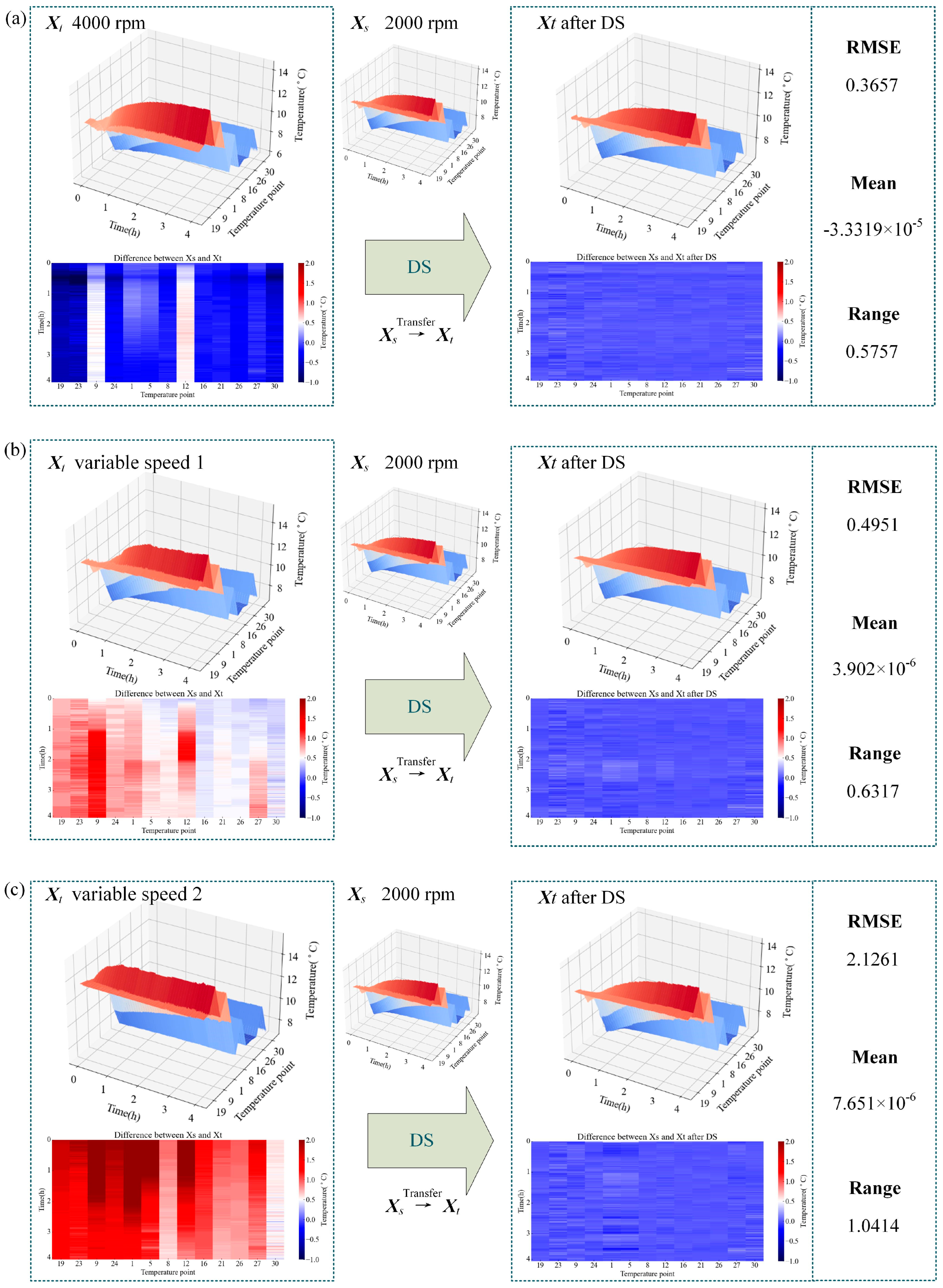
In order to verify the effect of domain adaptation in the improved DS correction method, transfer experiments were carried out using a source domain of 2000 rpm, target domain of 4000 rpm, variable speed 1, and variable speed 2. Those represent the three cases of fixed speed, simple variable speed, and complex variable speed, respectively.

The DS correction process is shown in Figure 13, where DS corrects the temperature characteristics of the target domain X_tto be similar to those of the source domain X_s. Due to the differences in the source and target domain distributions, the effectiveness of the classifier trained on the source domain applied to the target domain will be greatly reduced. The larger the difference, the less the model obtained from the training set can achieve good prediction results on the test set. When the target domain is 4000 rpm, the RMSE is only 0.3657 after DS spatial correction. When the target domain is variable speed 1, the RMSE is 0.4651 after DS spatial correction. When the target domain is variable speed 2, due to the excessive difference between the source and target domains, even if DS is used for spatial correction, the RMSE is 2.1261, which does not satisfy the transfer condition. After correction using DS, the extreme deviation of variable speed 1 is only 0.6317, while the extreme deviation of variable speed 2 is 1.0414. Although both are variable speeds, variable speed 1 has a longer duration of each stationary condition, and the working condition is less complicated compared to variable speed 2. Therefore, fixed speed and simple variable speed are more suitable for this model.

4.2. Validation of the Proposed Method

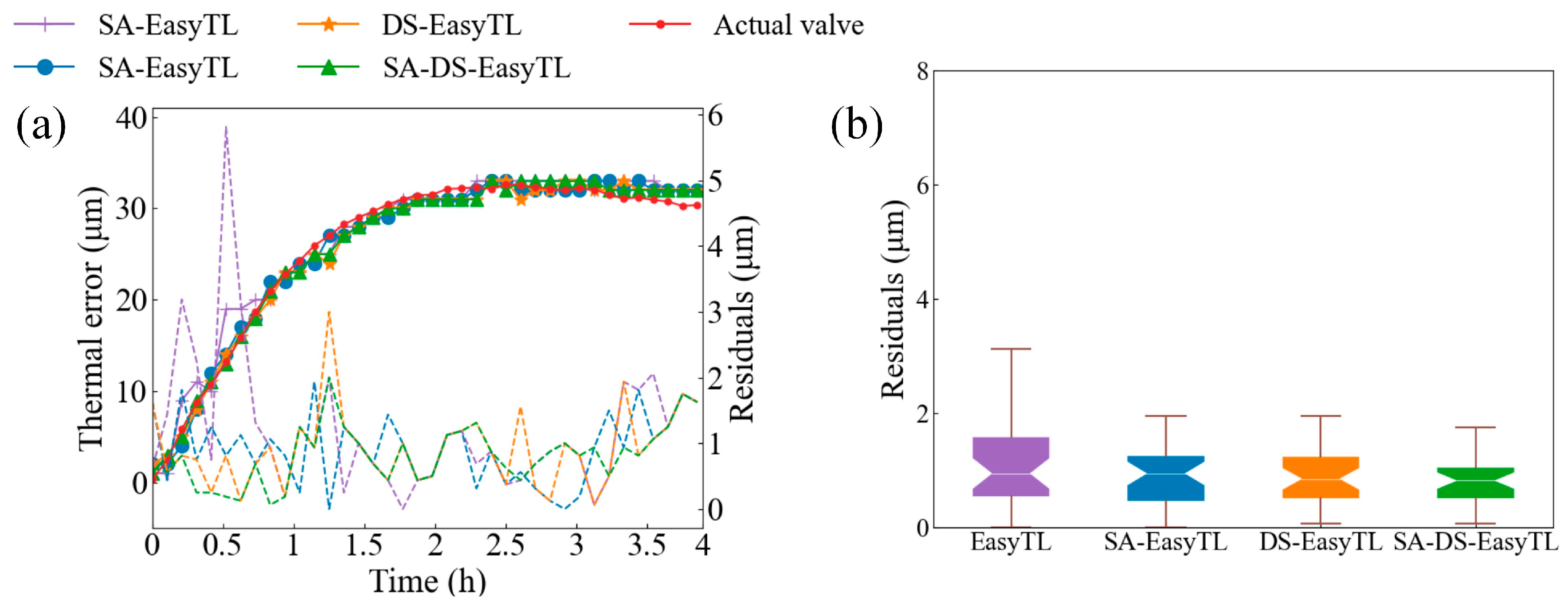
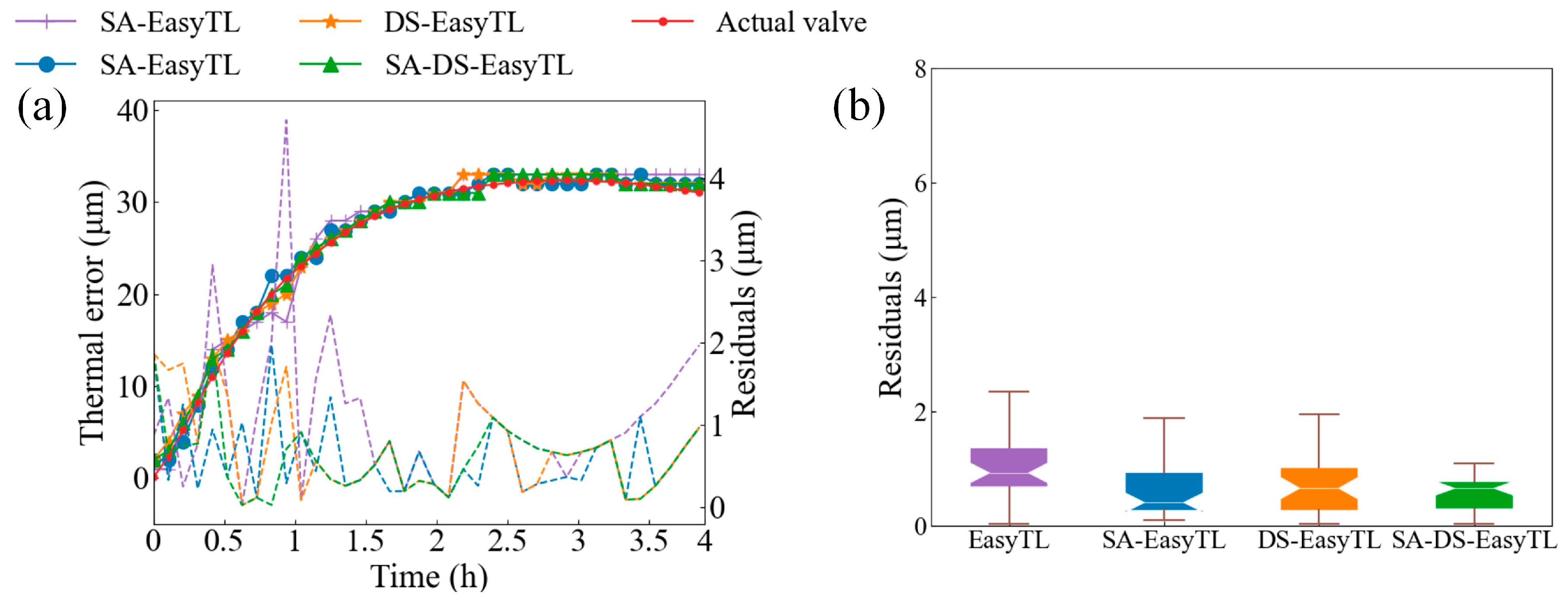
To explore the domain adaptation methods of the three EasyTL algorithms, SA-EasyTL, DS-EasyTL, and SA-DS-EasyTL, thermal error prediction was performed. With 2000 rpm as the source domain, the prediction results of the three EasyTL improvement models for 4000 rpm are shown in Figure 14. The mean error values of EasyTL, SA-EasyTL, DS-EasyTL, and SA-DS-EasyTL are 1.215 μm, 0.919 μm, and 0.817 μm, respectively. Compared to 2.605 μm² of EasyTL, 1.121 μm² of SA-EasyTL, and 1.184 μm² of DS-EasyTL, the MSE of SA-DS-EasyTL is only 0.865 μm². With 2000 rpm as the source domain, the prediction results of the three EasyTL improvement models for variable speed 1 are shown in Figure 15. The mean error values of SA-EasyTL, DS-EasyTL, and SA-DS-EasyTL are 1.648 μm, 2.016 μm, and 1.118 μm, respectively. Compared to 5.624 μm² of SA-EasyTL and 11.890 μm² of DS-EasyTL, the MSE of SA-DS-EasyTL is only 2.712 μm². The SA-DS-EasyTL model is more effective compared to the other two transfer models with one optimization algorithm, proving the established effectiveness of the model.

DS effectively narrows the distribution gap between the two domains, so that the knowledge learned by the model from the source domain can be efficiently transferred and applied to the data on the target domain, realizing the model’s adaption to new and unseen data. The main reason for the better performance of EasyTL is that there is basically not much difference between the target domain and the source domain in terms of features, which makes it relatively easy to use intra-domain alignment to realize the alignment between the target domain and the source domain. However, due to the significant differences in the multiple operating conditions and ambient temperatures of machine tools in practice, which will lead to large differences in the distribution of temperature features, it is difficult to compare the features between the source and target domains using the existing intra-domain comparison method in EasyTL. It is difficult to obtain the desired cross-disciplinary analysis results. Therefore, the combination of the attention mechanism and DS normalization was used to overcome the shortcomings of EasyTL.

4.3. Validation of the Transfer Feasibility

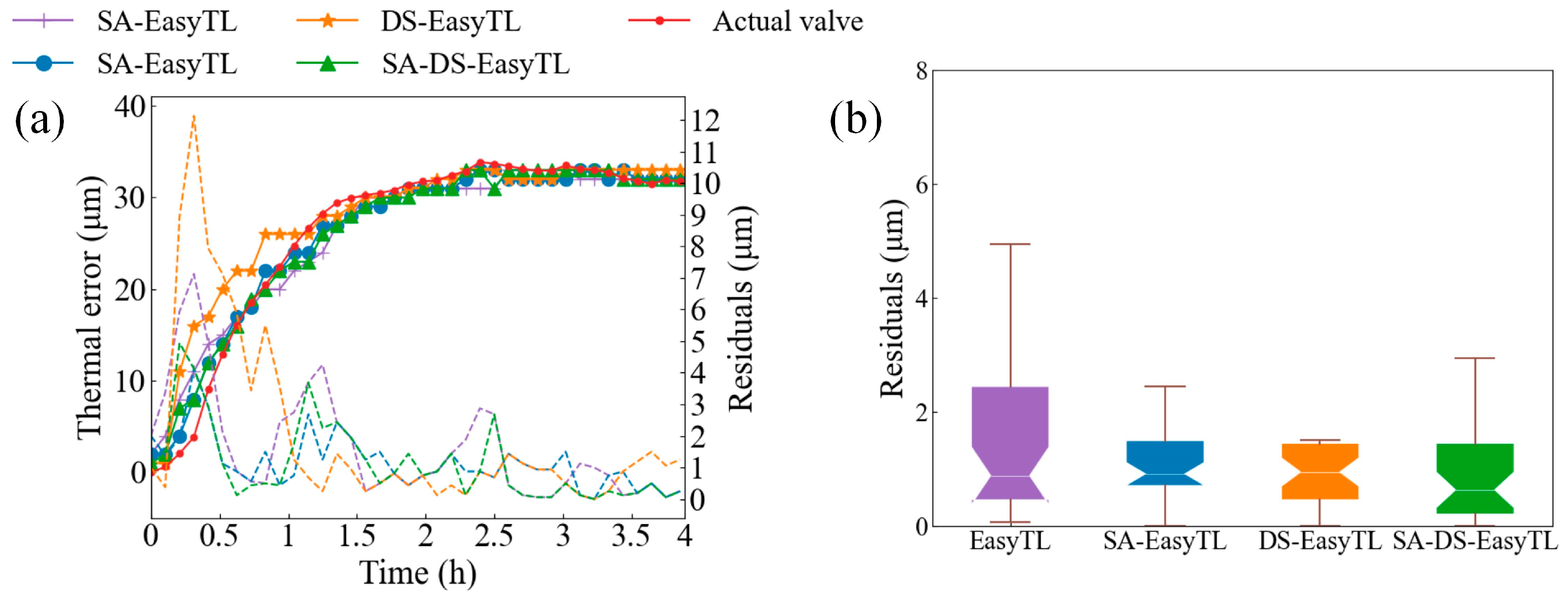
With 2000 rpm as the source domain, the prediction results of the four EasyTL improvement models for variable speed 2 are shown in Figure 16. The mean error values of EasyTL, SA-EasyTL, DS-EasyTL, and SA-DS-EasyTL are 2.513 μm, 1.829 μm, 1.161 μm, and 1.582 μm, respectively. Compared to 11.051 μm² of EasyTL, 5.013 μm² of SA-EasyTL, and 2.058 μm² of DS-EasyTL, the MSE of SA-DS-EasyTL is 5.624 μm². When the residuals account for more than 20% of the thermal error, it can be assumed that the difference between the source and target domains is too large to effectively accomplish knowledge transfer. When the source domain is 2000 rpm and the target domain is 2000 rpm, the residual difference accounts for 7.34% of the thermal error. When the source domain is 2000 rpm and the target domain is 4000 rpm, the residual difference accounts for 18.75% of the thermal error. When the source domain is 2000 rpm and the target domain is variable speed, the residual accounts for 39.3% of the thermal error. When the source domain is 4000 rpm and the target domain is variable speed, the residual accounts for 25.8% of the thermal error. The difference between the source and target domains is too large, which leads to poor model migration, so the proposed method is more suitable for knowledge transfer between fixed speeds.

5. Robust Validation of Transfer Model

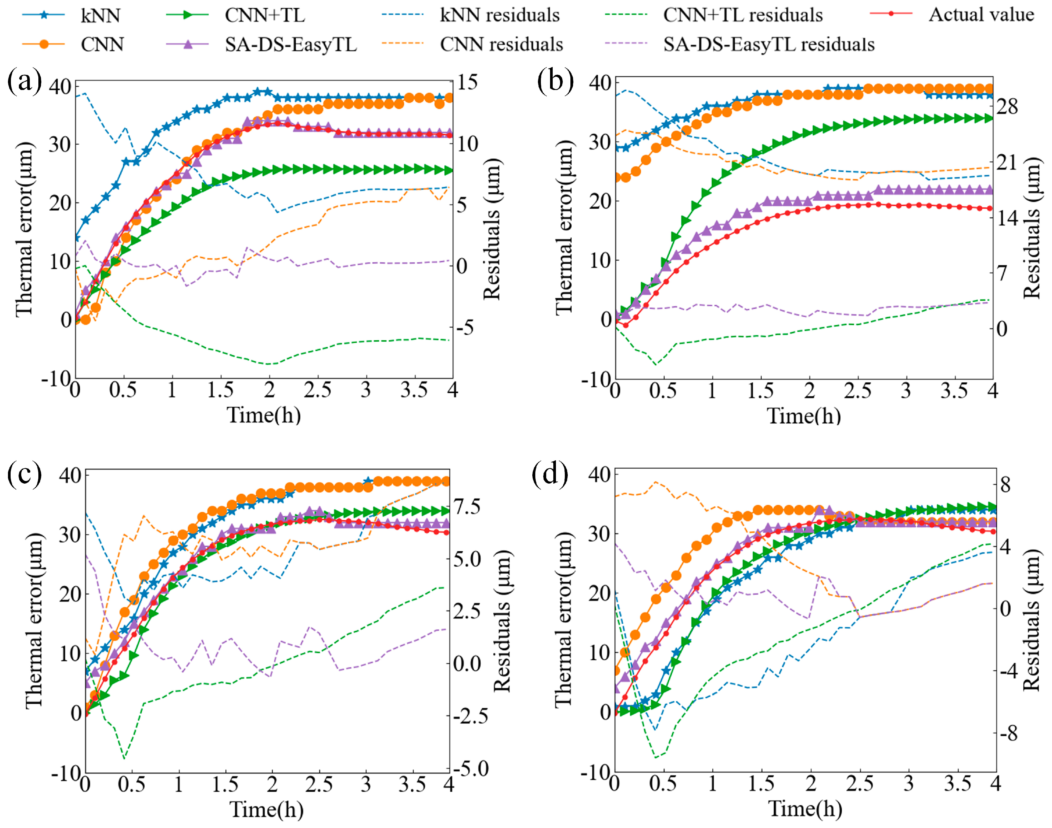
Machine learning k-nearest neighbor (kNN) and a deep learning convolutional neural network (CNN) were introduced for training and comparison. Based on the collected dataset, four experiments were designed, and the details are shown in

Table 1. Descriptions of the dataset.

Number	Dataset	Speed (rpm)	Working Condition
1	Training dataset	2000	Cold machine
	Test dataset	4000	Cold machine
2	Training dataset	2000	Cold machine
	Test dataset	4000	Not cold machine
3	Training dataset	2000	Cold machine
	Test dataset	Variable speed 1	Cold machine
4	Training dataset	Variable speed 1	Cold machine
	Test dataset	4000	Cold machine

. These three models were used to predict the four experiments, respectively, and the prediction results of the three models were compared.

Table 2. Comparison of training time for each model.

Model	KNN	CNN	CNN+TL	SA-DS-EasyTL
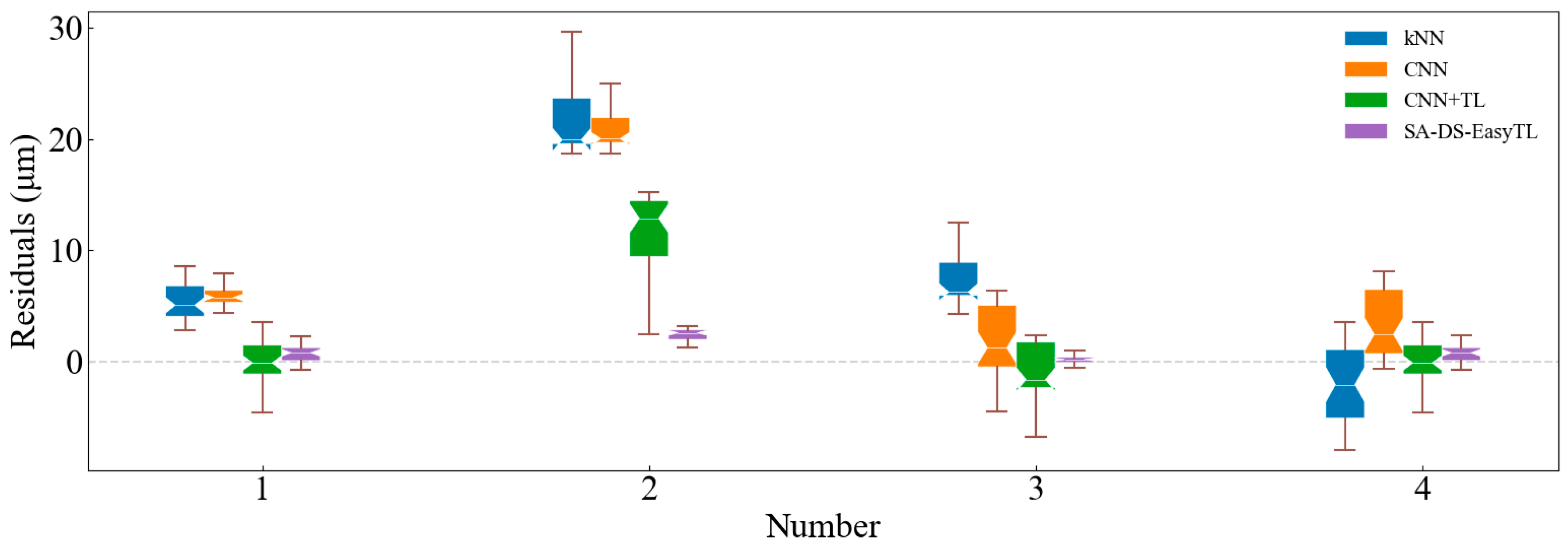
Time (s)	1.885	131.932	68.773	10.335

shows the training time of each model. The training time of the CNN with spatial alignment using DS for transfer learning (CNN+TL) is reduced by 48%, which proves that the in-domain alignment method can greatly improve the training efficiency of the model. kNN has the shortest training time because it is traditional machine learning. However, compared to the CNN and the CNN with transfer learning, SA-DS-EasyTL is only 10.335 s, with guaranteed prediction accuracy. From the prediction curves in Figure 17, SA-DS-EasyTL significantly outperforms kNN, the CNN, and the CNN with transfer learning in all four experiments (Figure 18). In the first experiment, the errors of the four models were kept within 10 μm because the difference between the working conditions of the training and test dataset was not very large, and SA-DS-EasyTL slightly outperformed the other three models. In contrast, when the gap between the training and test dataset was large, i.e., when the supervised information in the source domain was used to guide the label estimation in the target domain, a larger error occurred. As shown in the second experiment, the test dataset comes from an uncooled machine tool, and the temperature of the machine tool at time 0 is higher than that in the cold state. kNN, the CNN, and the CNN with transfer learning predict the thermal error directly from the prediction models trained at 2000 rpm; thus, the thermal error predicted by the two models is much higher than the actual thermal error. SA-DS-EasyTL reduces the difference in the distributions of the source and target domains, realizing transfer learning under different operating conditions. The predicted thermal error fluctuates around the actual values with acceptable differences. In the third variable speed experiment, the thermal errors of kNN and SA-DS-EasyTL show a decreasing trend after two hours, while the CNN is not sensitive. kNN, although sensitive to the variable speed change, has the largest prediction error among the three models under variable operating conditions. Similarly, SA-DS-EasyTL likewise performed the best in the experiments from variable to constant speed. This makes knowledge transfer possible with a small number of variable speed datasets. CNNs do not perform well with fewer samples as they require a large dataset to learn the relevant knowledge.

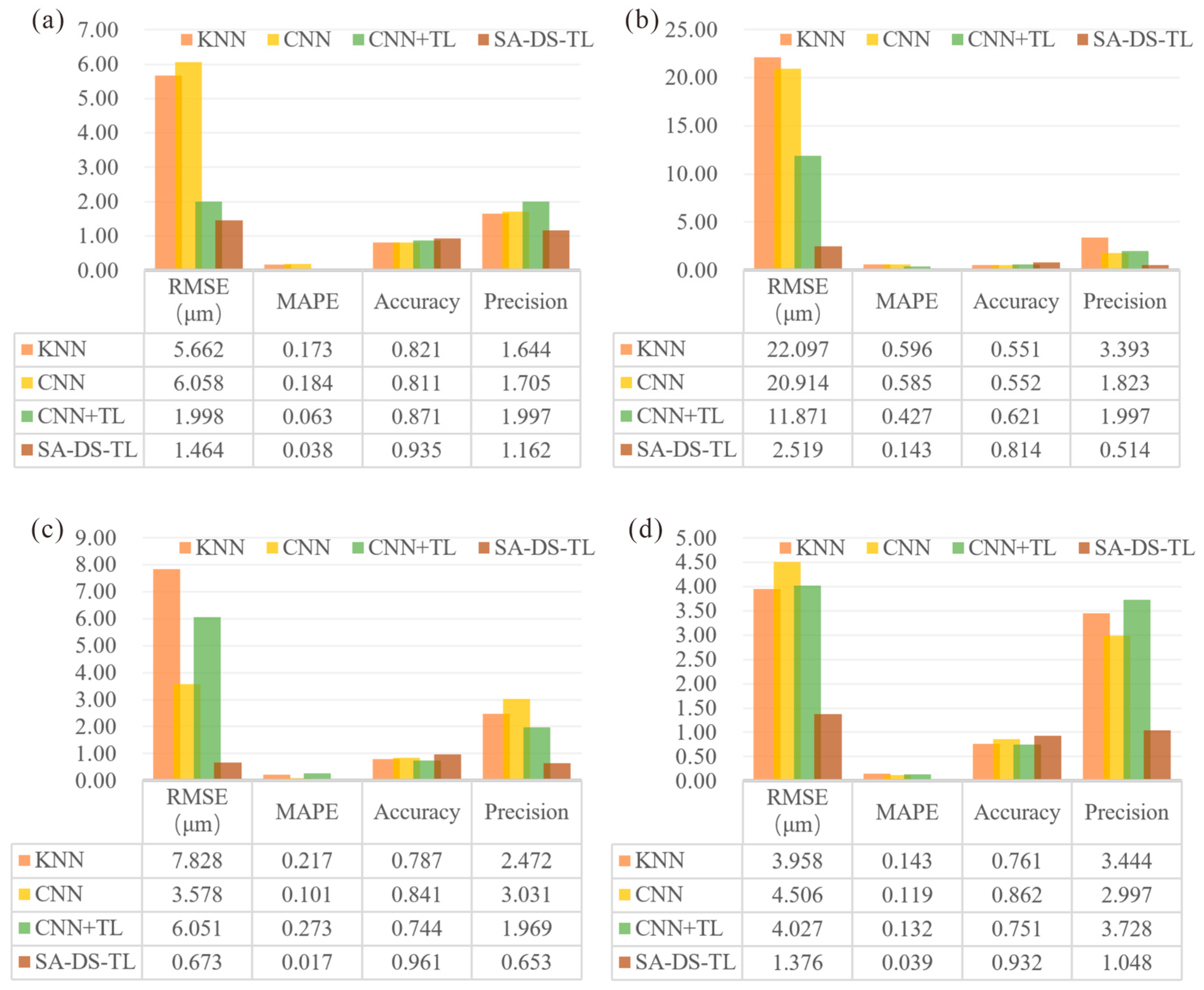
In this study, the above-mentioned four evaluation methods were used to evaluate and summarize the results predicted by three models. The results from the predicted results of the three models in the four experiments are shown in Figure 19. SA-DE-EasyTL has an MAPE of less than 0.1 in most experiments, and its accuracies are all minimized. Even in the second experiment, the RMSE is 2.519, and the accuracy is 0.814. In contrast, the RMSE of kNN, the CNN, and the CNN with transfer learning exceeds 20, and their accuracy is only around 0.55. After applying transfer learning to the CNN model, the prediction accuracy of the model also appeared to improve. In addition, the CNN method requires hyperparameter tuning when used, which undoubtedly makes it less efficient. This illustrates the advantages of EasyTL in terms of accuracy and efficiency because the performance of the classifier is highly dependent on good metric selection. When inappropriate metrics are used or the learned metrics are not suitable for different domains, the prediction performance will be severely degraded. Comparing the accuracy reflecting the degree of error dispersion, it can be found that transfer learning makes the prediction errors more concentrated and the thermal error prediction results more stable, which obviously improves the reliability of the prediction results.

6. Conclusions

In this paper, a thermal error model based on transfer temperature feature fusion is proposed. Temperature features were fused by self-attentive weights and used as inputs in the model. The fused features were subjected to domain adaptation based on an improved adaptive matrix of direct normalization. An EasyTL algorithm implements a nonparametric transfer model through in-domain pairs and in-domain programming learning to shorten the model training time and ensure the model prediction accuracy.

Firstly, sensitive temperature features were fused through a self-attention mechanism. The self-attentive mechanism assigns weights to the temperature information and fuses the obtained data with features. The feature fusion allows the data to contain good information and effectively extracts the hidden information in the data for the accurate modeling of thermal errors.

Secondly, an improved adaptive matrix method based on direct normalization was proposed to narrow the distribution gap between the source and target domains and improve knowledge transfer. By updating the background matrix with an autoencoder, the reconstructed adaptive matrix effectively transfers and applies the knowledge learned by the model from the source domain to the data in the target domain. A dataset suitability criterion was proposed to determine whether the test set is suitable for the improved adaptive matrix approach. The results show that the method is applicable to both constant and simple variable speed conditions validated for both transfer and non-transfer datasets.

Thirdly, with the advantages of EasyTL’s nonparametric and efficient learning, intra-domain alignment was performed to align the different feature distributions in the source and target domains. In thermal error experiments, the proposed SA-DS-EasyTL outperforms the traditional methods of kNN, a CNN, and a CNN with transfer learning. The CNN with transfer learning, due to the improved adaptive matrix, realizes the domain adaption, which shortens the training time of the model while improving the prediction accuracy of the model. By comparing the accuracy metrics reflecting the degree of error dispersion, it is found that the prediction errors of SA-DS-EasyTL are more concentrated, and the thermal error prediction results are more stable. This demonstrates the significant superiority of SA-DS-EasyTL in dealing with thermal error modeling problems requiring high accuracy and efficiency.

References

1. Mayr, J.; Jedrzejewski, J.; Uhlmann, E.; Donmez, M.A.; Knapp, W.; Härtig, F.; Wendt, K.; Moriwaki, T.; Shore, P.; Schmitt, R.; et al. Thermal issues in machine tools. CIRP Ann.-Manuf. Technol. 2012, 61, 771–791. [Google Scholar] [CrossRef]
2. Abdulshahed, A.M.; Longstaff, A.P.; Fletcher, S. The application of ANFIS prediction models for thermal error compensation on CNC machine tools. Appl. Soft Comput. 2015, 27, 158–168. [Google Scholar] [CrossRef]
3. Cheng, Y.; Zhang, X.; Zhang, G.; Jiang, W.; Li, B. Thermal error analysis and modeling for high-speed motorized spindles based on LSTM-CNN. Int. J. Adv. Manuf. Technol. 2022, 121, 3243–3257. [Google Scholar] [CrossRef]
4. Li, T.-J.; Sun, T.-Y.; Zhang, Y.-M.; Cui, S.-Y.; Zhao, C.-Y. Dynamic memory intelligent algorithm used for prediction of thermal error reliability of ball screw system. Appl. Soft Comput. 2022, 125, 109183. [Google Scholar] [CrossRef]
5. Yao, X.-H.; Fu, J.-Z.; Chen, Z.-C. Bayesian networks modeling for thermal error of numerical control machine tools. J. Zhejiang Univ.-Science A 2008, 9, 1524–1530. [Google Scholar] [CrossRef]
6. Clough, D.; Fletcher, S.; Longstaff, A.P.; Willoughby, P. Thermal Analysis for Condition Monitoring of Machine Tool Spindles. In Proceedings of the 25th International Congress on Condition Monitoring and Diagnostic Engineering (COMADEM), Huddersfield, UK, 18–20 June 2012. [Google Scholar]
7. Brecher, C.; Brozio, M.; Klatte, M.; Lee, T.H.; Tzanetos, F. Application of an Unscented Kalman Filter for Modeling Multiple Types of Machine Tool Errors. In Proceedings of the 50th CIRP Conference on Manufacturing Systems, Taichung, Taiwan, 3–5 May 2017; pp. 449–454. [Google Scholar]
8. Tan, F.; Yin, G.; Zheng, K.; Wang, X. Thermal error prediction of machine tool spindle using segment fusion LSSVM. Int. J. Adv. Manuf. Technol. 2021, 116, 99–114. [Google Scholar] [CrossRef]
9. Gui, H.; Liu, J.; Ma, C.; Li, M.; Wang, S. Mist-edge-fog-cloud computing system for geometric and thermal error prediction and compensation of worm gear machine tools based on ONT-GCN spatial–temporal model. Mech. Syst. Signal Process. 2023, 184, 109682. [Google Scholar] [CrossRef]
10. Chengyang, W.; Sitong, X.; Wansheng, X. Spindle thermal error prediction approach based on thermal infrared images: A deep learning method. J. Manuf. Syst. 2021, 59, 67–80. [Google Scholar] [CrossRef]
11. Chen, Y.; Zhou, H.C.; Chen, J.H.; Xu, G.D. Spindle thermal error modeling method considering the operating condition based on Long Short-Term Memory. Eng. Res. Express. 2021, 3, 035019. [Google Scholar] [CrossRef]
12. Sun, C.; Ma, M.; Zhao, Z.; Tian, S.; Yan, R.; Chen, X. Deep Transfer Learning Based on Sparse Autoencoder for Remaining Useful Life Prediction of Tool in Manufacturing. IEEE Trans. Ind. Inform. 2019, 15, 2416–2425. [Google Scholar] [CrossRef]
13. Zhu, M.; Yang, Y.; Feng, X.; Du, Z.; Yang, J. Robust modeling method for thermal error of CNC machine tools based on random forest algorithm. J. Intell. Manuf. 2022, 34, 2013–2026. [Google Scholar] [CrossRef]
14. Liao, Y.X.; Huang, R.Y.; Li, J.P.; Chen, Z.Y.; Li, W.H. Dynamic Distribution Adaptation Based Transfer Network for Cross Domain Bearing Fault Diagnosis. Chin. J. Mech. Eng. 2021, 34, 52. [Google Scholar] [CrossRef]
15. Katageri, P.; Suresh, B.S.; Pasha Taj, A. An approach to identify and select optimal temperature-sensitive measuring points for thermal error compensation modeling in CNC machines: A case study using cantilever beam. Mater. Today Proc. 2021, 45, 264–269. [Google Scholar] [CrossRef]
16. Zhang, X.; Yang, L.; Lou, P.; Jiang, X.; Li, Z. Thermal Error Modeling for Heavy Duty CNC Machine Tool Based on Convolution Neural Network. In Proceedings of the 2019 IEEE 3rd Information Technology, Networking, Electronic and Automation Control Conference (ITNEC), Chengdu, China, 15–17 March 2019. [Google Scholar]
17. Dai, Y.; Tao, X.; Xuan, L.; Qu, H.; Wang, G. Thermal error prediction model of a motorized spindle considering variable preload. Int. J. Adv. Manuf. Technol. 2022, 121, 4745–4756. [Google Scholar] [CrossRef]
18. Liu, J.; Ma, C.; Wang, S. Data-driven thermal error compensation of linear x-axis of worm gear machines with error mechanism modeling. Mech. Mach. Theory 2020, 153, 104009. [Google Scholar] [CrossRef]
19. Liu, M.; Gong, Y.; Sun, J.; Tang, B.; Sun, Y.; Zu, X.; Zhao, J. The accuracy losing phenomenon in abrasive tool condition monitoring and a noval WMMC-JDA based data-driven method considered tool stochastic surface morphology. Mech. Syst. Signal Process. 2023, 198, 110410. [Google Scholar] [CrossRef]
20. Xia, M.; Shao, H.; Williams, D.; Lu, S.; Shu, L.; de Silva, C.W. Intelligent fault diagnosis of machinery using digital twin-assisted deep transfer learning. Reliab. Eng. Syst. Saf. 2021, 215, 107938. [Google Scholar] [CrossRef]
21. Zhuang, F.Z.; Qi, Z.Y.; Duan, K.Y.; Xi, D.B.; Zhu, Y.C.; Zhu, H.S.; Xiong, H.; He, Q. A Comprehensive Survey on Transfer Learning. Proc. IEEE 2021, 109, 43–76. [Google Scholar] [CrossRef]
22. Pan, S.J.; Yang, Q.A. A Survey on Transfer Learning. IEEE Trans. Knowl. Data Eng. 2010, 22, 1345–1359. [Google Scholar] [CrossRef]
23. Liu, J.L.; Ma, C.; Gui, H.Q.; Wang, S.L. Transfer learning-based thermal error prediction and control with deep residual LSTM network. Knowl.-Based Syst. 2022, 237, 107704. [Google Scholar] [CrossRef]
24. Kuo, P.-H.; Tu, T.-L.; Chen, Y.-W.; Jywe, W.-Y.; Yau, H.-T. Thermal displacement prediction model with a structural optimized transfer learning technique. Case Stud. Therm. Eng. 2023, 49, 103323. [Google Scholar] [CrossRef]
25. Gao, M.; Qi, D.; Mu, H.; Chen, J. A Transfer Residual Neural Network Based on ResNet-34 for Detection of Wood Knot Defects. Forests 2021, 12, 212. [Google Scholar] [CrossRef]
26. Guo, L.; Lei, Y.; Xing, S.; Yan, T.; Li, N. Deep Convolutional Transfer Learning Network: A New Method for Intelligent Fault Diagnosis of Machines With Unlabeled Data. IEEE Trans. Ind. Electron. 2019, 66, 7316–7325. [Google Scholar] [CrossRef]
27. Wiessner, M.; Blaser, P.; Böhl, S.; Mayr, J.; Knapp, W.; Wegener, K. Thermal test piece for 5-axis machine tools. Precis. Eng.-J. Int. Soc. Precis. Eng. Nanotechnol. 2018, 52, 407–417. [Google Scholar] [CrossRef]
28. Hsieh, Y.L.; Cheng, M.H.; Juan, D.C.; Wei, W.; Hsu, W.L.; Hsieh, C.J. On the Robustness of Self-Attentive Models. In Proceedings of the 57th Annual Meeting of the Association-for-Computational-Linguistics (ACL), Florence, Italy, 28 July–2 August 2019; pp. 1520–1529. [Google Scholar]
29. Zhao, S.; Qiu, Z.; He, Y. Transfer learning strategy for plastic pollution detection in soil: Calibration transfer from high-throughput HSI system to NIR sensor. Chemosphere 2021, 272, 129908. [Google Scholar] [CrossRef]
30. Wang, J.; Chen, Y.Q.; Yu, H.; Huang, M.Y.; Yang, Q. Easy transfer learning by exploiting intra-domain structures. In Proceedings of the IEEE International Conference on Multimedia and Expo (ICME), Shanghai, China, 8–12 July 2019; pp. 1210–1215. [Google Scholar]
Figure 1. The position of sensors. (a) Temperature sensors. (b) Displacement sensors.
Machines 12 00728 g001
Figure 2. The measured data at variable speed 1. (a) Temperature data. (b) Thermal error data.
Machines 12 00728 g002
Figure 3. The measured data at variable speed 2. (a) Temperature data. (b) Thermal error data.
Machines 12 00728 g003
Figure 4. Flowchart of the thermal error prediction based on SA-DS-EasyTL.
Machines 12 00728 g004
Figure 5. (a) Dot-product attention. (b) Self-attention.
Machines 12 00728 g005
Figure 6. The framework of temperature feature fusion.
Machines 12 00728 g006
Figure 7. Attention weights for each temperature measurement point.
Machines 12 00728 g007
Figure 8. Prediction accuracy with feature fusion.
Machines 12 00728 g008
Figure 9. The result of feature fusion.
Machines 12 00728 g009
Figure 10. Autoencoder schematic diagram.
Machines 12 00728 g010
Figure 11. The framework of spatial correction.
Machines 12 00728 g011
Figure 12. Diagram of EasyTL.
Machines 12 00728 g012
Figure 13. Diagram of DS with source domain of 2000 rpm. (a) Target domain of 4000 rpm. (b) Target domain of variable speed 1. (c) Target domain of variable speed 2.
Machines 12 00728 g013
Figure 14. Prediction performance of different improved models with the target domain of 4000 rpm. (a) Comparison of prediction results. (b) Residual box plot.
Machines 12 00728 g014
Figure 15. Prediction performance of different improved models with the target domain of variable speed 1. (a) Comparison of prediction results. (b) Residual box plot.
Machines 12 00728 g015
Figure 16. Prediction performance of different improved models with the target domain of variable speed 2. (a) Comparison of prediction results. (b) Residual box plot.
Machines 12 00728 g016
Figure 17. Prediction results of thermal error. (a) 2000 rpm–4000 rpm. (b) 2000 rpm–4000 rpm (not cold machine). (c) 2000 rpm–variable speed 1. (d) Variable speed 1–4000 rpm.
Machines 12 00728 g017
Figure 18. Box plot of the residuals for four experiments.
Machines 12 00728 g018
Figure 19. Box plot of the residuals for four experiments. (a) 2000 rpm–4000 rpm. (b) 2000 rpm–4000 rpm (not cold machine). (c) 2000 rpm–variable speed. (d) Variable speed–4000 rpm.
Machines 12 00728 g019