Abstract
Within planetary gear transmissions (PGTs), mode shapes and eigenfrequencies hold a crucial significance in operational reliability and efficacy. Mode shapes explain the unique motion patterns inherent in PGT systems. Conversely, eigenfrequencies describe the inherent frequencies at which PGT systems undergo vibration or oscillation upon exposure to external forces or disruptions. This research paper presents a comprehensive investigation into the dynamic behavior of a three-stage PGT utilized in medium and heavy trucks. This study introduces the Rayleigh energy method to assess system dynamics, revealing a bounded Rayleigh quotient related to the highest related eigenvalue. Then, this study delves into eigenfrequencies and the mode shape behavior of the adopted PGT model. The eigenfrequencies are identified as encompassing diverse vibrational modes of central components and planet gears. Moreover, a multi-scale analysis of the adopted PGT model is presented by deriving matrices for mass, bearing stiffness, and mesh stiffness. Comparisons with the Rayleigh energy method demonstrate the new approach’s efficiency, exhibiting a low margin of error in the determination of eigenfrequencies. This investigation also highlights the alignment of identified mode shapes with the established literature, detailing the multi-scale approach’s minor deviation in mode shape determination compared to the Rayleigh energy method.
1. Introduction
PGT systems are crucial components in various mechanical systems, including wind turbines, automobiles, ships, aerospace, and other machinery, due to their compact construction, which enables higher transmission ratios within a smaller space compared to conventional gear systems. This compactness allows efficient space utilization and weight reduction, which are crucial in applications with space constraints. Additionally, PGT systems exhibit high efficiency due to multiple gear contacts distributing loads, resulting in reduced wear and improved durability. Their ability to evenly distribute forces among multiple gears contributes to a uniform load distribution, minimizing stress on individual components and enhancing overall reliability [1]. However, these advantages come with specific challenges. PGT systems demand precision in manufacturing and assembly due to their complex arrangement, which can increase production complexity and costs. Dynamic imbalance, particularly notable in configurations with numerous planet gears, poses challenges in achieving optimal performance.
Regarding the design of PGT systems, references [2,3,4,5] studied the multi-body dynamic modeling and analysis of PGT systems. Liu et al. [6] studied the dynamic analysis and characterization of a spur gear PGT system featuring journal bearings subjected to the influence of gravitational effects. Concli et al. [7] evaluated the validity of a planar lumped parameter model with 18 Degrees of Freedom (DOF) for the estimation of the system eigenfrequencies. A comprehensive dynamic model for a gear rotor bearing PGT system, integrating lateral and torsional nonlinearities, which encompassed multiple DOF, was also developed by [8,9,10].
Various modal analysis techniques are extensively employed to investigate the dynamic properties of a structure by extracting modal parameters in Mbarek et al. [11], where, in their study, they offer a comparative analysis of an experimental modal analysis test where an Operational Modal Analysis (OMA) test and an Order-based Modal Analysis (OBMA) test are applied to a recirculating energy PGT system. Modal and response harmonic analyses were conducted using ANSYS Workbench in reference [12] to explore the behavior of structures under varying boundary conditions. Their analysis technique provides insights into the eigenfrequencies and mode shape behavior of the structures, as well as their dynamic responses when subjected to harmonic excitations. Xu and Dong [13] investigated a heavy-duty PGT system using a 3D model utilized in trucks. The simulation module is developed for modal analysis of the system by using the Finite Element Method (FEM). Qian et al. [14] studied the inherent frequencies at which a PGT model system is utilized in a coal shearer, along with its corresponding modes of vibration, which provides crucial assistance in the formulation and supervision of the gear system’s design and operation. A comparison between frequency amplitude curves corresponding to various resonance modes, as well as an investigation into the impact of specific parameters on vibration amplitude, is presented by Zhang et al. [15]. Finally, the precision of their analytical solutions is assessed through numerical integration simulations.
Karray et al. [16] investigated the modal analysis and its characteristics of a two-stage helical PGT system used in a bucket wheel excavator. Tatar et al. [17] studied a six DOF model of a PGT rotor system using lumped parameter and FEM models, leading to the deduction that in the case of spur gear configuration, the vibration modes encompass axial, torsional, and lateral modes and those connected to each individual stage. In their work, Zhang et al. [18] presented a FEM model of PGT housing, considering the main factors affecting its dynamic characteristics through modal analysis. Kumar et al. [19] explored the impact of material mechanical properties on the natural frequencies and mode shapes of the PGT system within a heavy-duty vehicle gearbox. Both references [20,21] studied the modal analysis of helical gears. Brassitos and Jalili [22] investigate the vibration properties of planetary robotic PGT systems employing both the analytical method and FEM to extract its natural frequencies and corresponding mode shape behavior.
Berntsen et al. [23] used the eigenfrequencies obtained from OMA as center frequencies for the filter bands, and they proposed a method that defines which of the resonances most improves the fault. Kumar and Patil [24] constructed a FEM based on a numerical simulation method for a heavy-loaded vehicle truck PGT housing in order to find eigenfrequencies and mode shapes, and they determined the mode shapes for different transmission housing materials. In their paper, Ericson and Parker [25] analyzed the eigenfrequeny patterns of a PGT system where they congregate these eigenfrequency patterns into clusters characterized by similar frequencies. Each of these clusters encompassed a rotational, translational, and planet mode eigenfrequency. Also, It was concluded that these eigenfrequencies continue within their respective clusters even as system parameters undergo changes. Lin and Parker [26] defined the principles governing eigenvalue veering phenomena in PGT systems analytically. The interaction between neighboring eigenvalue loci is estimated using perturbation analysis techniques. Guo and Parker [27] examine the responsiveness of natural frequencies and vibration modes of a compound PGT system to changes in inertia and stiffness parameters. The resonance frequency of the system is determined in reference [28] by analyzing the lock-up oscillation data that occur at the gear shifting. The compliance of the output shaft is computed by evaluating the system’s resonance frequency. Reference [29] conducted a parameter analysis to investigate the influence of PGT design parameters on the overall modal behavior of PGT rotor systems. A three-dimensional dynamic model of a PGT rotor system is utilized to perform modal sensitivity analysis. The parameters examined include the number of planet gears, planet mistuning, the mass of planet gears, and planet gear speed. It was found that these parameters exhibit diverse effects on both the natural frequencies and mode shapes of the system. Stringer, Sheth, and Allaire [30] introduce a methodology for performing modal reduction on a dynamic system with a geared rotor, considering the influence of general damping and gyroscopic effects.
Based on the previous literature, this study investigates the dynamic behavior of a three-stage PGT model system employed in medium and heavy trucks, employing a lumped parameter model. Utilizing the Rayleigh energy method, the research examines the system’s dynamics, showing a constrained Rayleigh quotient associated with the highest eigenvalue, elucidating both natural frequencies and mode shape behavior. The identification of 63 natural frequencies provides complex insights into the vibrational characteristics of the PGT model system, encompassing a diverse spectrum of vibrational modes exhibited by central components and planet gears. Comparative assessments with the Rayleigh energy method show the multi-scale approach’s efficacy in capturing resonant characteristics.
2. Non-Linear Dynamic Modeling of a Three-Stage Planetary Gear Transmission System
The research object of this paper is a PGT model system utilized in medium and heavy-duty diesel trucks, its structure diagram is shown in Figure 1. The system has three stages. In the first stage, the ring gear is fixed to the gearbox housing, and each stage includes a sun gear , a ring gear , a planet carrier , and four planetary gears where is the number of the planets , four planets are carried in each stage where . The planetary stage number is or 3. Power is applied on the first stage sun gear . The first-stage carrier is connected to the second-stage ring . In addition, the second-stage carrier is connected to the third-stage ring . The third-stage carrier is connected to the output shaft. The PGT system employed in this study offers six-speed speed ratios utilized for medium and heavy trucks and these speed ratios could be achieved through adjustments to the fixed components. This investigation only focuses on a specific speed ratio, where the first-stage ring is fixed by being coupled to the gearbox body, as shown in Figure 1. The PGT model system parameters are provided in Table 1.
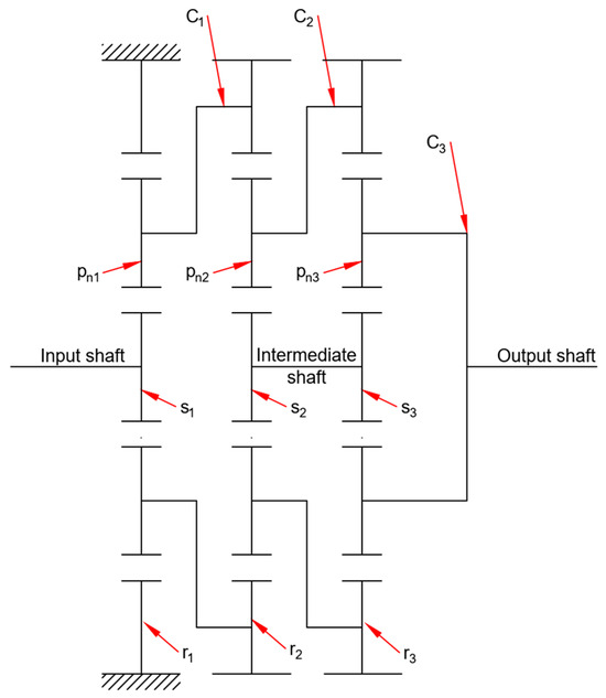
Figure 1.
Structure diagram of the adopted PGT model system.

Table 1.
Parameters of PGT model system.
Figure 2 represents the mathematical model of the adopted PGT system. The time-varying mesh stiffness (TVMS) represented by and , between sun–planet mesh connection and ring–planet mesh connection, are both presented in Equation (39), respectively. Bearing stiffness for sun gear, ring gear, planet carrier and planet gears along the -axis, -axis, and torsional axis are represented by , and , respectively, where and signify small translational displacements along the horizontal, vertical, and angular displacements around the coordinate origin in their respective coordinate systems, as shown in Figure 2. The circumferential orientation of each planet is represented by , where .
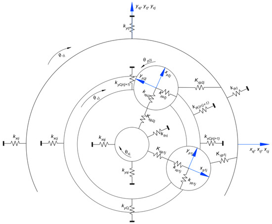
Figure 2.
Lumped parameter model of th stage for PGT model.
Given that the number of teeth on the sun gear and the ring gear are integer multiples of the number of the planets , . Hence, the relative phase angles are set to null. This deliberate adjustment is employed to equalize the distribution of load among the planets, ensuring balanced load sharing. Moreover, it results in the elimination of net forces transmitted from the planet gears to their respective supports, as elucidated by Parker [31]. This equilibrium in load distribution and force elimination within the system shows the interdependent relationships between gear parameters and their resultant effects on force transmission and distribution across PGT systems, as explained by Hu et al. [1].
The mathematical vibration model is described by Singiresu using the Lagrange equation as shown in Equation (1) as depicted in [32]:
where signifies the kinetic energy, represents the elastic potential energy function, is the generalized coordinate, is the generalized velocity of the , and is the generalized force vector; The kinetic energy function of the entire PGT model system can be calculated from Equation (2):
where , , and represent the kinetic energy functions of the th-stage sun gear, ring gear, and planet carrier, respectively. The kinetic energy function of the -th-stage sun gear can be mathematically expressed as follows:
where and represent the angular velocity and the relative phase angle respectively. signifies the installation eccentricity errors associated with the concerned gear. These errors signify deviations from the ideal positioning during the assembly or installation process. and represents the second moment of inertia and mass, respectively, subscript denotes one of the components .
The kinetic energy function of the -th-stage ring gear can be mathematically expressed as
The kinetic energy function of the th-stage carrier gear can be mathematically expressed as
The kinetic energy function of the th planet of the th stage can be mathematically expressed as
In the previous equations, , , and are the translational and torsional direction coordinates’ vibration velocities respectively, denotes the radius of the component . In this study, the connecting intermediate shaft, the connection between and , and the connection between and are simplified as springs with combined bending and torsional elasticities, as mathematically depicted in Equation (7). Consequently, the total elastic potential energy of the PGT system encompasses both the elastic potential energy of the bearings and PGT components and PGT system connections .
The bearing elastic potential energy function is identified as follows:
The elastic potential energy function can be mathematically represented as
where , , and represent the stiffness of the connecting shaft between the mentioned components, and represents the coordinate system, where . In order to employ the Rayleigh energy approach, the system, after solving Equations (1)–(9) using the lumped parameter model as demonstrated in references [33,34,35], is transformed into the matrix form where the PGT model system can be expressed as follows:
From the previous equation, represents the generalized coordinate expressed in Equation (11), while signifies the generalized acceleration. The matrices and are the generalized external forces, generalized mass, generalized stiffness matrices presented in Equations (12), (13), and (15) respectively. Superscript denotes to matrix transpose.
where , , and denotes the input torque to the PGT system, brake forces sybjected to , and represent the delivered torque from the PGT system. Equation (13) provides the total mass matrix formulation representing the entire PGT model system. Within this formulation, signifies the individual mass matrices of the first, second, and third stages of the system, describing the specific mass properties attributed to each stage.
Considering the homogeneity of each stage within the PGT model system, the equations presented will focus on the th stage. Equation (14) Reveals the components constituting the mass matrix terms, which are to be integrated into Equation (13).
Equation (15) displays the mathematical terms constituting the stiffness matrix. The unknowns of Equation (15) are shown in Appendix A.
3. Rayleigh Energy Method
The principle of the conservation of energy for vibrating systems can be stated in Equation (16).
where is the kinetic energy, and is the potential energy of an th DOF discrete system; for the present investigation, . The kinetic and potential energies can be expressed in Equations (17) and (18) respectively.
where represents the motion vector encompassing translational and rotational directions for each mode defined in Equation (19). The term denotes the generalized velocity vector of , while and stand for the generalized mass and stiffness matrices, respectively.
The vector is defined as a time-dependent function of vector of amplitudes . In order to determine the natural frequencies, a harmonic motion is assumed for the generalized coordinate , as presented in Equation (20).
where represents the natural frequency of vibration. By substituting Equation (20) into both Equations (17) and (18), the kinetic and potential energies can then be expressed as a function of natural frequency, as depicted in Equations (21) and (22) respectively.
Given the PGT system’s conservativeness, the equality between the maximum kinetic energy and the maximum potential energy can be inferred from Equation (23):
Upon substitution of both Equations (21) and (22) into Equation (23), the eigen frequencies of the system can be obtained in Equation (24):
The expression on the right-hand side of Equation (24) represents the Rayleigh quotient, mathematically denoted .
3.1. Properties of Rayleigh’s Quotient
has a static value in the vicinity of any eigenvector . To demonstrate this, the arbitrary vector can be expressed in terms of the normal modes of summation of eigenvectors as follows:
where denotes the coefficient of the mode shape . Then, by substituting from Equation (25) into Equations (21) and (22), Equations (26) and (27) are obtained.
From Equations (23), (26), and (27) then by considering the orthogonality property, it becomes apparent that and will equate to zero for
From both Equations (24) and (28), the Rayleigh quotient can be mathematically expressed as follows:
When the normal modes are subjected to normalization, then Equation (29) transforms into Equation (30), depicting the altered expression of the Rayleigh quotient.
If varies slightly from the eigenvector , then the coefficient will notably exceed the remaining coefficients of . Consequently, Equation (30) can be reformulated mathematically as follows:
Given that is an infinitesimal value, then by considering , where represents an extremely small numerical value for all . Consequently, Equation (31) can be formulated as
Equation (32) indicates that if the arbitrary vector slightly differs from the eigenvector by a small quantity of the first order, then the Rayleigh quotient differs from the eigenvalue by a small quantity of the second order. This signifies that Rayleigh’s quotient exhibits a stationary value in the neighborhood of an eigenvector. This value is petite in the vicinity of the fundamental mode . In order to investigate this further, consider setting in Equation (31) and refer to Equation (32). Then, Equation (33) is concluded.
In view of the fact that , then Equation (33) leads to Equation (34). This proves that the Rayleigh quotient is never lower than the first eigenvalue, which establishes a clear boundary. By advancing in a comparable approach, Equation (34) can demonstrate that the Rayleigh quotient is in no way higher than the highest eigenvalue. Thus, the Rayleigh quotient defines both an upper bound of and a lower bound of .
3.2. System Mode Shapes
In this study, the system mode shapes have been thoroughly investigated, encompassing various vibrational modes of the central components and planet gears within the adopted PGT model system. The following investigation illustrates the most distincit five vibration modes of the adopted PGT model obtained based on the characteristics of the vibration shape. The mode shape vector represented as will be used to allocate each individual vibrational mode.
3.2.1. Central Components’ Pure Torsional Vibrational Mode
In this mode shape vector, the vibrational behavior of all central gears are primarily dominated by torsional vibrations with minor translational vibrations. Through the analysis of the mode shape vector, it is evident that the main vibrational motion of the central gears is torsional in nature and can be described as follows:
The distribution of gears within the PGT model system during the pure torsional vibrational mode of the central components is depicted in Figure 3.
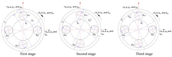
Figure 3.
Component allocations of the central components’ pure torsional vibrational mode.
3.2.2. Central Components’ Pure Translational Vibrational Mode
The analysis of this mode shape vector reveals that the PGT central gears exhibit significant translational motion along both x-coordinate and y-coordinate directions, as shown in Figure 4. These translational motions have implications on the PGT system dynamic response, affecting its overall displacement and response to external forces. Furthermore, a minor component of rotational vibration in the -coordinate direction is observed in the mode shape vector. -coordinate vibrations are less obvious compared to translational vibrations. Hence, torsional vibrations will be disregarded in the mode shape vector analysis, the mode shape vector analysis can be presented as follows:
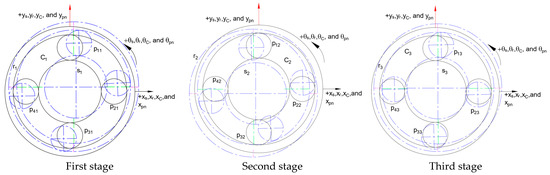
Figure 4.
Component allocations of the central components’ pure translational vibrational mode.
The distribution of gears within the adopted PGT model system during the pure translational vibrational mode of the central components is depicted in Figure 4.
3.2.3. First-Stage Planet Gear Vibrational Mode
In the mode vector, the vibrational amplitudes of both translational and torsional components for the central components of the second and third stages are negligible. Moreover, the vibrations observed in the first-stage sun gear, ring gear, and planet carrier are relatively minor compared to the vibrations experienced by the planet gears of the same stage. The analysis of the mode shape indicates that the dominant vibrational motion is primarily confined to the planet gears of the first stage. This behavior signifies that the planet gears are more sensitive to vibrational excitations compared to other components of the PGT model system.
The negligible vibrations of the central components in the second and third stages further contribute to the PGT system overall stability and reliable operation. This simplification simplifies the modeling process and can lead to significant computational savings as follows:
The distribution of gears within the adopted PGT model system during the first-stage planet gear vibrational mode is depicted in Figure 5.
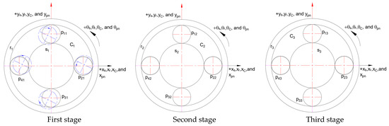
Figure 5.
Component allocations of the first-stage planet gear vibrational mode.
3.2.4. Second-Stage Planet Gear Vibrational Mode
In this mode vector, the translational and torsional vibrations of the central components of the first and third stages are negligible. In the second stage, the sun gear, ring gear, and planet carrier experience minor vibrations, but these vibrations are considerably lower in amplitude when compared to the vibrations observed in the planet gears within the same stage. This phenomenon can be explained by the lack of consideration for the vibrations present within these shafts, where the vibrations triggered by these components are not included in the analysis. Consequently, gear and gear are not externally affected by any source of vibrations, leading to their negligible vibrational amplitudes in the mode vector.
The dominance of the second-stage planet gears in terms of vibrational amplitude can be attributed to the interactions and load-sharing mechanisms within the PGT model system. The planet gears in the second stage are crucial in transmitting torque and absorbing load, making them more prone to vibrations compared to other components.
The distribution of gears within the adopted PGT model system during the second-stage planet gear vibrational mode is depicted in Figure 6.
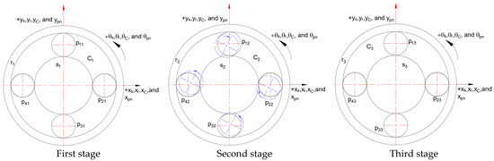
Figure 6.
Component allocations of the second-stage planet gear vibrational mode.
3.2.5. Third-Stage Planet Gear Vibrational Mode
In the mode vector, the translational and torsional vibrations of the central components in the first and second stages are negligible. For the third stage, the planet gears vibrations cannot be neglected, where
The distribution of gears within the adopted PGT model system during the third-stage planet gears vibrational mode is depicted in Figure 7.
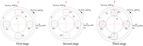
Figure 7.
Component allocations of the third-stage planet gear vibrational mode.
4. Multi-Scale Analysis of Lateral-Torsion-Coupling Dynamics of Planetary Gear Transmission
This paper provides a comparison between both the Rayleigh energy method and the multiscale approach for calculating eigenfrequencies and determining the mode shapes. In order to acquire the multi-scale analysis of lateral-torsion-coupling dynamics of PGT model system, the following analysis will take place. Equation (35) elucidates the differential equation governing dynamics inherent in the PGT model system. This equation encapsulates the complex relationship between lateral and torsional movements.
where corresponds to the mass matrix encapsulating the adopted PGT model system mass distribution across its components, as presented in Appendix B. refers to the bearing stiffness matrix. Additionally, stands for the TVMS matrix. Both and represent the stiffness characteristics within the PGT components and interconnections over time, as detailed in Appendix B. denotes the force exerted on each DOF presented in Equation (12). Vector is composed of the displacement of each component of the system, as expressed in Equation (11). Then, the periodic change in the TVMS can be obtained from Equation (36).
where and are the mean meshing stiffness of both external–external mesh and external–internal mesh connections of the PGT model presented in Table 1, respectively. Both and represent the order Fourier coefficients of the TVMS. stands for the corresponding conjugate plurals. Fourier expansions are expressed for and in Equation (37).
In the preceding two equations, and represent the overlap degrees. and are the peak-to-peak values of sun–planet meshing stiffness and ring–planet meshing stiffness, respectively. and represent the degree of coincidence, as shown in Figure 8. is the meshing period. To justify this, the sun–planet mesh stiffness and ring–planet mesh stiffness of the PGT model are then expressed in the form of Fourier series by assuming Equations (38).
where is an infinitesimal parameter. By substituting both Equation (38) into Equation (36), TVMS between sun–planet mesh and ring–planet mesh connections can be found in Equation (39), respectively.
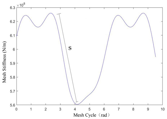
Figure 8.
Time-varying mesh stiffness diagram.
By substituting both Equations (39) into Appendix B, then, Equation (40) is found:
Both expressions define the respective modal deformations for the sun–planet mesh and ring–planet mesh connections, respectively. and denotes the mesh stiffness of the connection between sun-planet mesh and ring-planet mesh respectively where they are the constitution matricies of and their detailed formulations are provided in Appendix B.
Upon converting Equation (40) from cartesian coordinates to modal coordinates and by considering , Equation (41) emerges as a result. This transformation allows for the representation of gear meshing characteristics in a modal domain, facilitating a more comprehensive analysis of the PGT model system dynamic behavior and responses.
where , , , and . Furthermore, the periodic vibration frequency of the system can be expanded as a power series of a small amount , as provided in Equation (42).
By introducing a series of time scales , , then the system th-order response can be approximated, as depicted in Equation (43). This methodology enables the PGT model system behavior to be analyzed across different time frames, allowing for a comprehensive understanding of its responses and dynamics at varying temporal intervals. These time scales refer to different frequencies within the adopted PGT model system. For eigenfrequency analysis, different modes of vibration or eigenfrequencies occur at different temporal scales, representing the PGT system dynamic behaviour.
The analysis now is focused on the first-order approximation solution of the system of the system, requiring the addition of only two time scales. Equation (44) represents the th order of the modal response solution of the system, capturing the system’s behavior and response in relation to its modal characteristics within this approximation.
Hence, the vibration potential energy and vibration kinetic energy between the same vibration order are transferred. By substituting Equations (43) and (44) into Equation (41), Equation (45) can be concluded.
where and are elements of the th row and th column of matrices and , respectively. is the order harmonic amplitude and initial phase. Both expressions and are provided in the following Equations (46) and (47) respectively:
Then, the partial derivative operator of the multi-scale method is defined in Equations (48) and (49) as follows:
In the previous two equations, and are being used as counters. By substituting Equations (44), (48), and (49) into Equation (45), then comparing the same power of the subsequent partial differential Equation (50) can be achieved:
By considering the main resonance as the analysis object, Equation (51) can be introduced.
The frequency relationship of the main resonance can be expressed as , where is a small misalignment offset parameter, assuming is not an integer multiple of . Then, Equation (52) can be concluded.
As evidenced by both equations expressed in (52), the primary resonant reaction of the system aligns with an excitation characterized by a corresponding period. Moreover, the magnitude of this primary resonant response is influenced by simultaneous disturbance frequencies within the PGT model system, resulting in a modulatory relationship with the primary excitation frequency. Building upon the preceding analysis and recognizing that the PGT system meshing frequency holds greater potential for exciting system resonance, the investigation into the principal resonance phenomenon of the system is conducted on the foundation of the PGT system meshing excitation.
The term in Equation (52) represents the meshing frequency that affects the vibration response of the system. With the intention of further characterizing the influence of the meshing phenomenon on the vibration response of the system, the expression can be expanded mathematically, as shown in Equation (53).
By substituting Equations (50) and (51) into Equation (49) and considering the condition of eliminating the infinite terms, Equation (54) can be derived for the -th order mode.
By substituting Equation (53) into both Equations (52) and after simplification, Equation (55) is achieved.
Upon delving into the first-order harmonic assessment, the -th order modal vibration response introduces the first-order ordinary differential equations, as demonstrated in Equation (56). These equations encapsulate the determination of the amplitude and phase of where is an infinesmal parameter for the -order modal vibration response.
Upon additional elaborating on Equation (56); then Equation (57) is acquired in mode shapes . This derived equation offers insights into the system mode shape dynamics described by .
By taking into consideration the arithmetic expression for parameter then, Equation (58) is attained.
4.1. System Natural Frequency
By comparing both of the eigenfrequencies obtained from both the Rayleigh energy approach obtained in Equation (24) and the multi-scale approach from Equation (58), Figure 9 is plotted, which presents a comprehensive comparative analysis between them. The focal point of this investigation is the precision in detecting the eigenfrequencies by the multi-scale method. Upon particular examination of the obtained results, it becomes evident that the proposed method exhibits an error margin of approximately 2.5% deviation from the Rayleigh energy method in accurately identifying the eigenfrequencies. This inconsistency highlights the efficacy and potential of the multi-scale method in enhancing the precision of angular frequency detection when compared to the Rayleigh energy method.
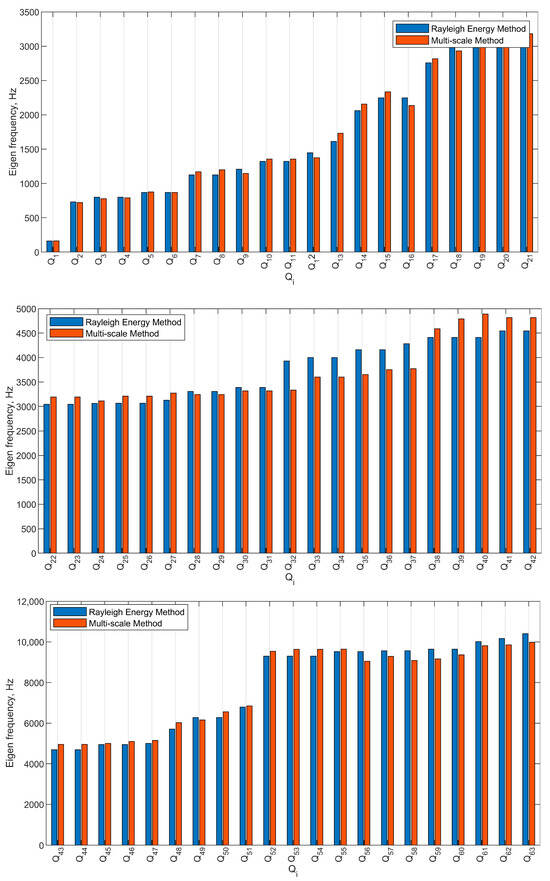
Figure 9.
Comparison between eigenfrequency allocation using both approaches: Rayleigh energy and multi-scale.
Figure 9 shows the allocation of the 63 eigenfrequencies in correlation with the DOF. The x-axis represents the eigenfrequency number , mirroring the corresponding number of DOF. Each point along the x-axis correlates to a distinct mode shape, linking it to the rotational speed at which the particular eigenfrequency occurs. This presentation offers a comprehensive mapping of eigenfrequencies to the adopted PGT system’s DOF, providing insights into specific mode shapes and their association with rotational speeds.
4.2. Mode Shapes
Figure 10 illustrates the torsional vibration vectors of the central components, depicting the pure torsional vibrational mode present in each stage. By referring to Section 3.2.1, the analysis of this mode shape vector extends to identify significant torsional motion along the -coordinate direction in the PGT central gears. Further analysis shows the presence of torsional vibrations within planet gears as well. The analysis of the mode shapes reveals that gears occupying similar positions within their respective stages share nearly identical vibrational patterns. This phenomenon is evident across the stages, indicating a consistent and repetitive vibrational behavior among gears within the same stage as follows:
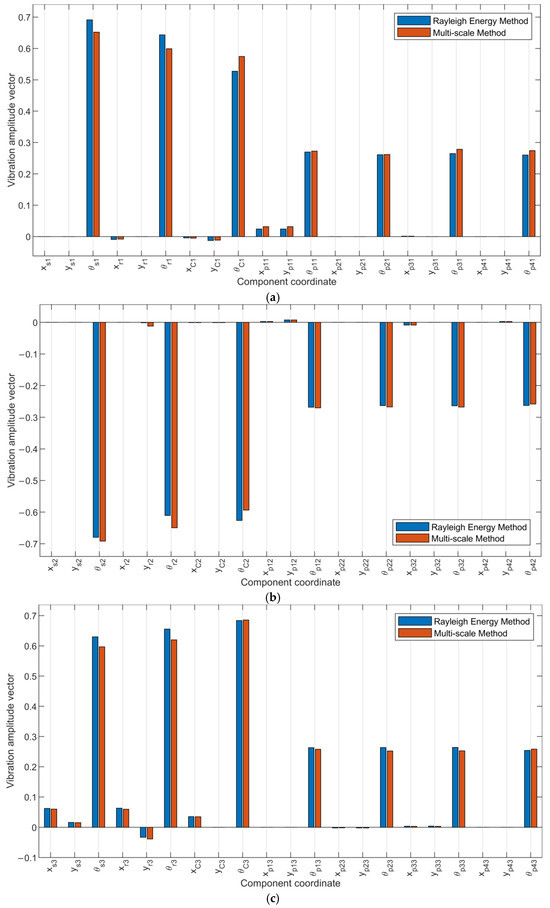
Figure 10.
Mode shape vector for central components’ pure torsional vibrational mode. (a), (b), and (c) referes to first, second, and third stages respectively.
Figure 11 display the vibration vectors of the central components for the pure translational vibrational mode in each stage. By referring to Section 3.2.2, the analysis of this mode shape vector extends to reveal substantial translational motion along both the x-coordinate and y-coordinate directions in the PGT central gears. In this mode shape, it cannot be guaranteed that the displacement of the central parts of the th stage is equal in magnitude to stage. However, certain patterns in the displacements can be observed among stages. Specifically, it is observed that the displacements of the first and third stages are in the same direction, indicating a coherent behavior between these stages. In contrast, the displacement of the second stage is 180° out of phase with the first and third stages, signifying an opposite vibrational response.
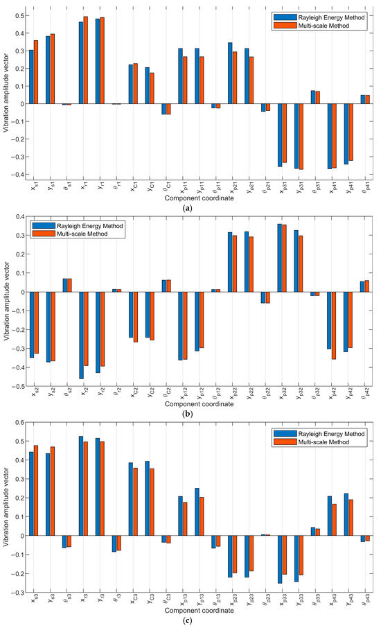
Figure 11.
Mode shape vector for central components’ pure translational vibrational mode. (a), (b), and (c) referes to first, second, and third stages respectively.
Furthermore, based on the analysis of the presented mode shape, it can be concluded that the mode shape of the planet gears within the same stage but positioned 180 degrees apart exhibit a remarkable similarity in magnitude while being opposite in direction. The examination of the mode shape of the planet gears within the same stage reveals a symmetrical vibrational pattern. Specifically, when comparing the mode shapes of two planet gears positioned 180 degrees apart from each other within the same stage, their magnitudes are approximately equivalent. However, the direction of their vibrational motion is opposite as follows:
For the first stage,
For the second stage,
For the third stage,
Figure 12 demonstrate the mode shape behavior specific to the first stage planetary gear vibrational mode. Figure 12 exclusively showcase significant vibrations within the first stage while omitting other stages due to their minimal vibration levels, ensuring clarity in presentation. Furthermore, by referring to Section 3.2.3 and based on the analysis of the presented mode shape, it can be concluded that the mode shape of the planet gears within the first stage but positioned 180 degrees apart exhibit a remarkable similarity in magnitude and direction as follows:

Figure 12.
Mode shape vector for first-stage planet gear vibrational mode.
Figure 13 demonstrate the mode shape behavior specific to the second stage planetary gear vibrational modes, respectively. Figure 13 exclusively showcase significant vibrations within the second stage while omitting other first and third due to their minimal vibration levels, ensuring clarity in presentation. Furthermore, by referring to Section 3.2.4 and based on the analysis of the presented mode shape, the following can be observed:
Figure 13.
Mode shape vector for second-stage planet gear vibrational mode.
Figure 14 demonstrate the mode shape behavior specific to the third stage planetary gear vibrational modes. Figure 14 exclusively showcase significant vibrations within the third stage while omitting other stages due to their minimal vibration levels, ensuring clarity in presentation. Furthermore, by referring to Section 3.2.5 and based on the analysis of the presented mode shape, the following can be observed:
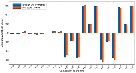
Figure 14.
Mode shape vector for third-stage planet gear vibrational mode.
Figure 10, Figure 11, Figure 12, Figure 13 and Figure 14 provide a comprehensive comparative analysis between the established Rayleigh energy approach and the recently introduced multi-scale approach, specifically focusing on the entirety of mode shape vectors. This investigation is aimed at understanding the inconsistencies in performance between the two approaches across various modes of vibration. The error magnitudes, expressed as percentages, stand at 5.1%, 3.1%, 6.2%, 6.8%, and 10.05% for the pure torsional vibrational mode, pure translational vibrational mode with central components, first-stage planet gear vibrational mode, second-stage planet gear vibrational mode, and third-stage planet gear vibrational mode, respectively. These quantified inconsistencies provide valuable insights into the effectiveness of the multi-scale approach in capturing the complex characteristics of different vibrational modes.
5. Conclusions
This paper starts with establishing the lumped parameter model of a three-stage PGT utilized in medium and heavy trucks by introducing the potential and kinetic energies inherent in the system. Subsequently, it delves into the theory of the Rayleigh energy method, a robust tool for assessing the dynamic behavior of the system by deriving matrices for mass, bearing stiffness, and mesh stiffness. Afterward, the Rayleigh quotient for the PGT model system was derived, and it was proved that the Rayleigh quotient is bounded by the highest eigenvalue, shedding light on the PGT model system inherent natural frequencies and mode shapes.
Furthermore, this investigation proceeds to discuss the natural frequencies of the entire system, revealing a total of 63 eigenfrequencies, offering a comprehensive analysis that elucidates the vibrational characteristics of the PGT model system. Examining the adopted PGT model mode shapes, this study encompasses diverse vibrational modes of both central components and planet gears.
Additionally, this paper presents the multi-scale analysis for the adopted PGT model system. This study rigorously compares the multi-scale analysis approach with the well-established Rayleigh energy method to evaluate its efficiency and reliability in capturing the complex resonant characteristics and mode shape vectors inherent in the system’s behavior. This study’s conclusions present significant findings as follows:
- The identified mode shapes align with those found in T.M. and R.G. Parker [25], encompassing whole system torsional and translational vibrational modes, torsional and translational vibrational modes of central components, and torsional and translational planet modes.
- The multi-scale approach demonstrates a margin of error in the amplitude of approximately 2.5% in accurately determining eigenfrequencies compared to the Rayleigh energy method.
- The error magnitudes, expressed as percentages, stand at 5.1%, 3.1%, 6.2%, 6.8%, and 10.05%, highlighting deviations in the determination of the pure torsional vibrational mode, pure translational vibrational mode with central components, first-stage planet gear vibrational mode, second-stage planet gear vibrational mode, and third-stage planet gear vibrational mode, respectively.
Author Contributions
Conceptualization, M.M. and Y.X.; methodology, M.M. and K.Y.; software, M.M. and Q.Y.; validation, M.M., K.Y. and P.G.; formal analysis, M.M. and Q.Y.; investigation, M.M. and Y.X. resources, M.M. and K.Y.; data curation, M.M. and Q.Y.; writing—original draft preparation, M.M.; writing—review and editing, M.M. and P.G.; visualization, M.M.; supervision, M.M. and P.G.; project administration, M.M. and P.G.; funding acquisition, M.M. and P.G. All authors have read and agreed to the published version of the manuscript.
Funding
This research paper is sponsored by VTDP Project (Nos. DLZX202304 and 202302329249); Key Laboratory Stable Support Project (No. 202320301483).
Data Availability Statement
All the related data have been provided within this paper.
Conflicts of Interest
The authors declare no conflicts of interest. The funders had no role in the design of the study; in the collection, analyses, or interpretation of data; in the writing of the manuscript; or in the decision to publish the result.
Appendix A
In all the following equations and
Appendix B
References
- Hu, Y.; Talbot, D.; Kahraman, A. A load distribution model for planetary gear sets. J. Mech. Des. 2018, 140, 053302. [Google Scholar] [CrossRef]
- Zhu, D.; Li, Z.; Hu, N. Multi-Body Dynamics Modeling and Analysis of Planetary Gearbox Combination Failure Based on Digital Twin. Appl. Sci. 2022, 12, 12290. [Google Scholar] [CrossRef]
- Yang, W.; Tang, X. Modelling and modal analysis of a hoist equipped with two-stage planetary gear transmission system. Proc. Inst. Mech. Eng. Part K J. Multi-Body Dyn. 2017, 231, 739–749. [Google Scholar] [CrossRef]
- Chen, R.; Qin, D.; Liu, C. Dynamic modelling and dynamic characteristics of wind turbine transmission gearbox-generator system electromechanical-rigid-flexible coupling. Alex. Eng. J. 2023, 65, 307–325. [Google Scholar] [CrossRef]
- Inalpolat, M.; Kahraman, A. Dynamic modelling of planetary gears of automatic transmissions. Proc. Inst. Mech. Eng. Part K J. Multi-Body Dyn. 2008, 222, 229–242. [Google Scholar] [CrossRef]
- Liu, Z.; Liu, Z.; Yu, X. Dynamic modeling and response of a spur planetary gear system with journal bearings under gravity effects. J. Vib. Control 2018, 24, 3569–3586. [Google Scholar] [CrossRef]
- Concli, F.; Cortese, L.; Vidoni, R.; Nalli, F.; Carabin, G. A mixed FEM and lumped-parameter dynamic model for evaluating the modal properties of planetary gearboxes. J. Mech. Sci. Technol. 2018, 32, 3047–3056. [Google Scholar] [CrossRef]
- Li, W.; Sun, J.; Yu, J. Analysis of dynamic characteristics of a multi-stage gear transmission system. J. Vib. Control 2019, 25, 1653–1662. [Google Scholar] [CrossRef]
- Geng, Z.; Li, J.; Xiao, K.; Wang, J. Analysis on the vibration reduction for a new rigid–flexible gear transmission system. J. Vib. Control 2022, 28, 2212–2225. [Google Scholar] [CrossRef]
- Al-Shyyab, A.; Alwidyan, K.; Jawarneh, A.; Tlilan, H. Non-linear dynamic behaviour of compound planetary gear trains: Model formulation and semi-analytical solution. Proc. Inst. Mech. Eng. Part K J. Multi-Body Dyn. 2009, 223, 199–210. [Google Scholar] [CrossRef]
- Mbarek, A.; Del Rincon, A.F.; Hammami, A.; Iglesias, M.; Chaari, F.; Viadero, F.; Haddar, M. Comparison of experimental and operational modal analysis on a back to back planetary gear. Mech. Mach. Theory 2018, 124, 226–247. [Google Scholar] [CrossRef]
- Mohsine, A.; Boudi, E.; El Marjani, A. Investigation of structural and modal analysis of a wind turbine planetary gear using finite element method. Int. J. Renew. Energy Res. 2018, 8, 752–760. [Google Scholar]
- Xu, Z.; Dong, Y. Modal analysis of transmission gear in gearbox based on SolidWorks. In Proceedings of the 2011 Second International Conference on Mechanic Automation and Control Engineering, Inner Mongolia, China, 15–17 July 2011; pp. 413–416. [Google Scholar]
- Qian, P.-Y.; Zhang, Y.-L.; Cheng, G.; Ge, S.-R.; Zhou, C.-F. Model analysis and verification of 2K-H planetary gear system. J. Vib. Control 2015, 21, 1946–1957. [Google Scholar] [CrossRef]
- Zhang, L.; Wang, C.; Bao, W.; Xie, F. Three-dimensional dynamic modeling and analytical method investigation of planetary gears for vibration prediction. Proc. Inst. Mech. Eng. Part K J. Multi-Body Dyn. 2021, 235, 37–56. [Google Scholar] [CrossRef]
- Karray, M.; Feki, N.; Khabou, M.T.; Chaari, F.; Haddar, M. Modal analysis of gearbox transmission system in bucket wheel excavator. J. Theor. Appl. Mech. 2017, 55, 253–264. [Google Scholar] [CrossRef][Green Version]
- Tatar, A.; Schwingshackl, C.W.; Friswell, M.I. Dynamic behaviour of three-dimensional planetary geared rotor systems. Mech. Mach. Theory 2019, 134, 39–56. [Google Scholar] [CrossRef]
- Zhang, T.; Shi, D.; Zhuang, Z. Research on vibration and acoustic radiation of planetary gearbox housing. In Proceedings of the INTER-NOISE and NOISE-CON Congress and Conference Proceedings, Melbourne, Australia, 16–19 November 2014; pp. 1319–1328. [Google Scholar]
- Kumar, A.; Jaiswal, H.; Jain, R.; Patil, P.P. Free vibration and material mechanical properties influence based frequency and mode shape analysis of transmission gearbox casing. Procedia Eng. 2014, 97, 1097–1106. [Google Scholar] [CrossRef][Green Version]
- Sheng, Z.; Tang, J.; Chen, S.; Hu, Z. Modal Analysis of Double-Helical Planetary Gears With Numerical and Analytical Approach. J. Dyn. Syst. Meas. Control 2015, 137, 041012. [Google Scholar] [CrossRef]
- Karray, M.; Feki, N.; Chaari, F.; Haddar, M. Modal analysis of helical planetary gear train coupled to bevel gear. In Proceedings of Mechatronic Systems: Theory and Applications: Proceedings of the Second Workshop on Mechatronic Systems JSM’2014; Springer: Cham, Switzerland, 2014; pp. 149–158. [Google Scholar]
- Brassitos, E.; Jalili, N. Dynamics of integrated planetary geared bearings. J. Vib. Control 2020, 26, 565–580. [Google Scholar] [CrossRef]
- Berntsen, J.; Brandt, A.; Gryllias, K. Enhanced demodulation band selection based on Operational Modal Analysis (OMA) for bearing diagnostics. Mech. Syst. Signal Process. 2022, 181, 109300. [Google Scholar] [CrossRef]
- Kumar, A.; Patil, P.P. Modal analysis of heavy vehicle truck transmission gearbox housing made from different materials. J. Eng. Sci. Technol. 2016, 11, 252–266. [Google Scholar]
- Ericson, T.M.; Parker, R.G. Natural frequency clusters in planetary gear vibration. J. Vib. Acoust. 2013, 135, 061002. [Google Scholar] [CrossRef]
- Lin, J.; Parker, R.G. Natural frequency veering in planetary gears. Mech. Struct. Mach. 2001, 29, 411–429. [Google Scholar] [CrossRef]
- Guo, Y.; Parker, R.G. Sensitivity of general compound planetary gear natural frequencies and vibration modes to model parameters. J. Vib. Acoust. 2010, 132, 011006. [Google Scholar] [CrossRef]
- Lee, T.H.; Choi, S. Modeling and Parameter Estimation of Automatic Transmission for Heavy-Duty Vehicle Using Dual Clutch Scheme; SAE Technical Paper 2020-01-2242; SAE International: Warrendale, PA, USA, 2020. [Google Scholar]
- Tatar, A.; Schwingshackl, C.W.; Friswell, M.I. Modal sensitivity of three-dimensional planetary geared rotor systems to planet gear parameters. Appl. Math. Model. 2023, 113, 309–332. [Google Scholar] [CrossRef]
- Stringer, D.; Sheth, P.; Allaire, P. Modal reduction of geared rotor systems with general damping and gyroscopic effects. J. Vib. Control 2011, 17, 975–987. [Google Scholar] [CrossRef]
- Parker, R.G. A physical explanation for the effectiveness of planet phasing to suppress planetary gear vibration. J. Sound Vib. 2000, 236, 561–573. [Google Scholar] [CrossRef]
- Singiresu, S.R. Mechanical Vibrations; Addison Wesley: Boston, MA, USA, 1995. [Google Scholar]
- Zghal, B.; Graja, O.; Dziedziech, K.; Chaari, F.; Jablonski, A.; Barszcz, T.; Haddar, M. A new modeling of planetary gear set to predict modulation phenomenon. Mech. Syst. Signal Process. 2019, 127, 234–261. [Google Scholar] [CrossRef]
- Yan, P.; Li, Y.; Gao, Q.; Wang, T.; Zhang, C. Research on the Coupled Phase-Tuning Vibration Characteristics of a Two-Stage Planetary Transmission System. Machines 2023, 11, 610. [Google Scholar] [CrossRef]
- Gao, P.; Liu, H.; Yan, P.; Xie, Y.; Xiang, C.; Wang, C. Research on application of dynamic optimization modification for an involute spur gear in a fixed-shaft gear transmission system. Mech. Syst. Signal Process. 2022, 181, 109530. [Google Scholar] [CrossRef]
Disclaimer/Publisher’s Note: The statements, opinions and data contained in all publications are solely those of the individual author(s) and contributor(s) and not of MDPI and/or the editor(s). MDPI and/or the editor(s) disclaim responsibility for any injury to people or property resulting from any ideas, methods, instructions or products referred to in the content. |
© 2024 by the authors. Licensee MDPI, Basel, Switzerland. This article is an open access article distributed under the terms and conditions of the Creative Commons Attribution (CC BY) license (https://creativecommons.org/licenses/by/4.0/).