Development of a Simulator for Household Refrigerator Using Equation-Based Optimization Control with Bayesian Calibration

Abstract

Conventional household refrigerators consist of a motor-driven compressor, evaporator, condenser, and expansion valve. To determine the optimal operation strategies of refrigerators, it is essential to investigate the overall system performance, using an appropriate simulator. This study proposed a data-driven simulator based on engineering features and machine learning algorithms for conventional household refrigerators. The most correlated variables for identifying the indoor temperature of refrigerators were identified using variable importance, and these were revealed to be the circulation fan speed, compressor operation status, and refrigerant flow direction. A data-driven simulator was constructed using Bayesian calibration, which considers the important variables, combined with a straightforward heat balance equation. The Markov Chain Monte Carlo approach was used to simultaneously calibrate three coefficients on the critical variables based on the heat balancing equation on each time step, which is consistent with the actual temperature of the container. The results revealed that the proposed approach (equation-based Bayesian calibration outperforms) standard machine learning algorithms, such as linear regression and random forest models, by 38.5%. Additionally, compared to the typical numerical analysis method, it can reduce the delivery time and effort required to develop a reliable simulator for household refrigerators.

1. Introduction

In 2004, Cemagref and ANIA evaluated the cold chain in France to monitor the temperature of a process from its initial manufacture to its final consumption [1]. They found that 40% of items, such as iced products, low-temperature live food, and pharmaceuticals, which require consistent temperature, were not being stored at the appropriate temperature in domestic refrigerators. The internal temperatures of household refrigerators are predicted using deterministic models that rely on precise information about the coefficients, initial conditions, and operating conditions. However, these assumptions do not align with the actual practices of consumers, such as thermostat settings, ambient temperature, and loading. Additionally, the working conditions are subject to stochastic fluctuations [2].

The air circulation and the number of items stored in a refrigerator result in the fluctuation of its internal temperature; thus, it is classified as a variable of unpredictability. These variables can be described using statistical measures, such as average, variation, and probability density. Several studies have examined heat transmission in vacant residential refrigerators [2,3,4], but less research has been conducted on object-filled refrigerators. Research on object-filled refrigerators can provide a valuable understanding of the anomalies in the temperature and velocity under various conditions. Laguerre et al. [5] replicated the behavior of static refrigerators under both empty and loaded conditions using a physics-based model based on computational fluid dynamics (CFD), while also considering the effects of radiation. They observed the presence of circular airflow patterns around the sides of the refrigerator, as well as the influence of height on the temperature. However, despite its potential as a valuable simulation technique, the high time requirement of CFD has constrained its further application [5].

Studies have evaluated the application of the most advanced numerical methodologies for simulating the behavior of refrigerators. For example, Hermes and Melo comprehensively assessed the transient modeling of refrigerators [6] and concluded that the transitory approach is the most suitable strategy for simulating the whole refrigerator system, owing to its ability to accurately represent the real behavior. Accordingly, they created and evaluated an accurate semi-empirical model for a two-compartment refrigerator, using a transient approach. However, Hermes et al. [7] reported that, in addition to the energy loss that occurs during the transient approach owing to the cyclic operation, it requires extensive computing resources, limiting its practical design or optimization. Despite the challenges in empirically measuring the losses related to cycling working mode, they can be estimated using a transient methodology. The use of a steady-state technique has the advantage of the shortest simulation time, but this is accompanied by significantly reduced accuracy. Given that this approach relies on the assumption that the air within compartments maintains a constant temperature, it can only provide an approximate estimation of the dynamic outcomes, such as the run time ratio.

The complexities associated with the design of refrigeration systems have prompted the exploration of more efficient modeling methodologies to meet the requirements of the industry. Additionally, refrigeration systems have been modeled and optimized using various artificial intelligence approaches over the years. Some of the most applicable approaches are expert systems; heuristic algorithms, such as genetic algorithms; and fuzzy logic [8]. To improve the responsiveness and resilience of a refrigeration system in various operational environments, studies [9,10] have employed the fuzzy logic principles to enhance the system’s control, and researchers are currently investigating methods that can be employed to reduce the energy consumption of ACs [11,12,13].

In addition, various artificial intelligence techniques have been employed over time to simulate and enhance refrigeration systems. Prabha et al. [14] analyzed the effect of many factors on the functioning of refrigeration and cooling systems, using mathematical models that consider the evaporating and condensing temperatures, as well as the mass of the refrigerant charge. Wei-le et al. [15] developed a predictive model for the coefficient of performance of a fridge in a supermarket, and another study simulated a micro-cooling system using a neural network [16]. They estimated three commonly used energy metrics using the neural network as a function of the evaporation and condensation temperatures.

The use of both deterministic and stochastic models is a widely employed approach in food product process engineering owing to the potential variability in product attributes and the uncertainty surrounding process circumstances [17]. This technique is often used in the thermal processing of packaged goods. Studies have proposed several methodologies to quantify the influence of unknown model parameters on the output of a system. Products inside the cold chain are often exposed to unforeseen variables, such as temperature fluctuations and storage duration in refrigeration system. Also, one of stochastic models uses Bayesian calibration. Bayesian calibration (inverse uncertainty quantification) has been successfully applied to many other stochastic modeling and calibration fields. The methodology is quite mature, and the innovations are mainly from customizing the solutions to different fields [18,19,20,21].

The precise prediction of the inner temperature of a refrigerator offers advantages not only to preserving the freshness of the product but also in enhancing the machine control for domestic equipment. Thus, implementing a development system that enables rapid testing and validation of new control logic in a virtual setting, while also ensuring a development environment that accurately represents various external conditions and new experiments, can effectively reduce costs. Moreover, using a projected model to simulate the isothermal condition and evaluate its general application in thermodynamics, can extend the ability of the predictive model to accommodate and manage loads and their activities [22].

The selection of the appropriate refrigerant and control strategy is crucial in the development of a high-performance system. To achieve this, it is essential to perform empirical studies to comprehensively understand the utilization habits of customers and energy efficiency under different storage conditions. However, this increases the time and cost required to obtain a universal result. Hence, dependable simulation models may aid in cost reduction and time savings, while helping in the design and optimization of heat exchangers [23,24,25].

This study aimed to construct a model that can simulate temperature variations within a refrigerator that uses compressor power and fan frequency control. This is based on the fact that numerous experiments are required to construct a refrigerator model in reality. However, there are challenges that hinder the construction of deterministic models, such as CFD or new mathematical models, by repeating the experiments [26,27,28,29,30]. To address this issue, in this study, a refrigerator simulation model based on a hybrid stochastic model with a Bayesian calibration was constructed. Furthermore, there are certain complexities associated with a refrigerator model that cannot be handled solely through mathematical formulas or CFD, including system efficiency degradation and unpredictable factors, such as external temperature influx when the refrigerator door is opened or closed. These factors hinder the development of a refrigerator simulation model. Therefore, an innovative refrigerator simulation model based on an actual refrigerator model was developed to address these challenges.

This study presents a novel approach for the derivation of a data-driven model of a household refrigerator. The proposed approach can reduce the time and effort required to develop an appropriate simulator for predicting and estimating the performance of appliances. The developed model was validated by demonstrating its effectiveness in scenarios, including temperature variations through the refrigerator operation conditions. The rest of this paper is organized as follows: In Section 2, the system descriptions of the target household refrigerator and the theoretical fundamentals of three potential simulator models are presented. The collected data based on conventional usage patterns and the prediction performance evaluation of three different models are presented in Section 3. All findings and future works are summarized in Section 4.

2. Methodology

2.1. System Description

The system analyzed in this study is a household double-door refrigerator with two compartments. The whole system was studied as two sub-systems, including cabinets and refrigeration loops. The compartments in the refrigerators include cabinets and freezers, which are specifically designed to preserve food items at either 4 or −18 °C. The fresh-food section is located at the top section of the refrigerator, whereas the freezer is located below. Detailed information on the specifications of the refrigerator is shown in

Table 1. Specifications of the refrigerator.

Elements	Contents
Capacity (L)	727
LED light (-)	Yes
Interior cabin door (-)	Yes
Compressor type (-)	Linear
Fast freeze mode (-)	Yes
Hygiene fresh (-)	Yes
2 Drawers (-)	Yes
Multi-airflow (-)	Yes
Dimension (mm)	902 (W) × 1785 (H) × 920 (D)

. Despite being thermally insulated, these compartments are connected via one wall and can be considered independent units. It should be noted that the compartment doors are assumed to be closed at all times for the simulation.

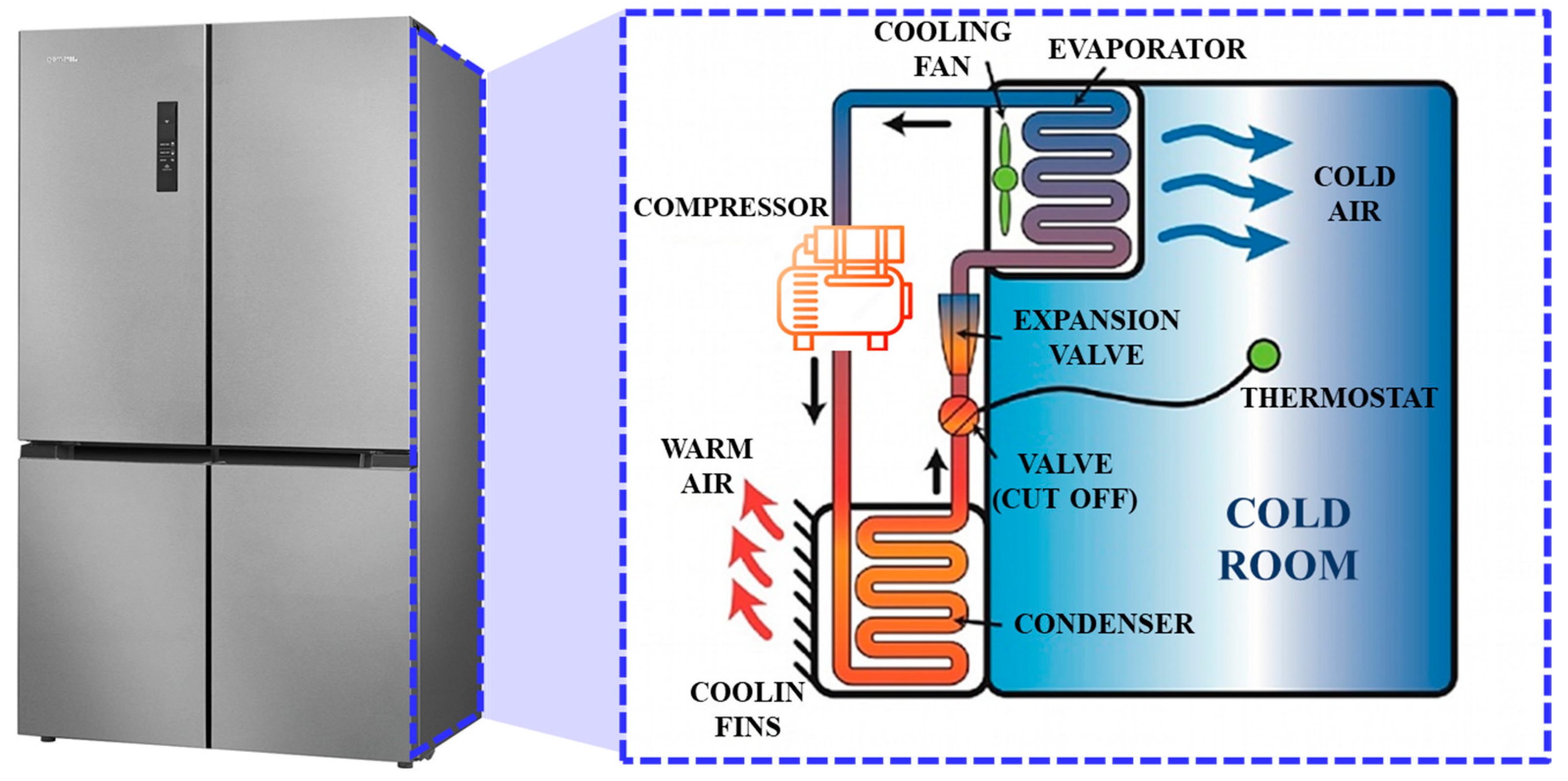
The refrigeration loop is a mechanism involving the use of a vapor compression system to cool the cabinets. The refrigeration loop shown in Figure 1 consists of a single-speed reciprocating hermetic compressor, a finned-tube no-frost evaporator, a natural draft wire-and-tube condenser, and a concentric capillary tube-suction line heat exchanger [31].

The temperature of air in the fresh-food and freezer compartments is regulated through the control of the damper, fan, and compressor. The freezer’s temperature is the only factor that determines whether the compressor is on or off. A centrifugal fan in the freezer cabinet distributes air to both the freezer and fresh-food cabinets via a distribution system. When the compressor is functioning, the fan runs continuously, and it consists of a single-speed motor.

2.2. Data Preprocessing

After collecting the input and output data of the refrigerator, the input and output data were preprocessed. Data preprocessing is a crucial phase in the machine learning pipeline, playing a pivotal role in enhancing the performance and robustness of models. This section discusses the key aspects of data preprocessing, including normalization, data scaling, and other relevant techniques. Normalization is a fundamental step to ensure that the scale of all features in the dataset is consistent, preventing certain variables from dominating others during the model training process. This is particularly important when dealing with diverse datasets with features spanning different ranges. Common normalization techniques include the following:

Min–max scaling transforms data into a specific range, typically [0, 1], preserving the relationships between data points, while mitigating the impact of outliers [32].

$$X_{normalized}=\frac{X-X_{min}}{X_{max}-X_{min}}$$

(1)

Z-score normalization standardizes data by transforming them into a distribution with a mean of 0 and a standard deviation of 1, making them suitable for algorithms sensitive to the scale of features [33].

$$X_{standardized}=\frac{X-\mu }{\sigma }$$

(2)

In addition to scaling and normalization, addressing missing data is imperative for building robust models. Strategies include imputation; removal of instances; or leveraging advanced techniques, such as data augmentation.

2.3. Feature Engineering

This study employed the Pearson correlation coefficient approach to identify the characteristics of the data input. This approach, often used to assess the linear correlations between two variables, entails dividing the covariance of the variables by the product of their standard deviations. Correlation, which is a standardized form of covariance assuming a normal distribution, is denoted by ‘r’ for the sample correlation coefficient and ‘ρ’ for the population correlation coefficient. The formula for the Pearson correlation coefficient is given below [34]:

$$\mathrm{Pearson} \mathrm{Correlation} {\rho }_{X,Y}=\frac{cov(X,Y)}{{\sigma }_X{\sigma }_Y}$$

(3)

The Pearson correlation coefficient quantifies the degree of linear association between two variables, X and Y. The calculation involves determining the covariance between the standardized versions of variables X and Y. The coefficient is dimensionless, indicating that it is independent of the scale of the variables. The range of values ranges from −1 to +1. A value of −1 represents a perfect negative correlation, +1 represents a perfect positive correlation, and 0 represents no correlation.

Cohen [35] described the Pearson correlation coefficient and proposed three effect sizes for the coefficient: small, medium, and huge. The classification of the effect sizes is as follows: a correlation value of 0.1 represents a small impact size, 0.3 represents a medium effect size, and 0.5 represents a big effect size. Cohen clarified that a medium effect size indicates a correlation that is likely to be perceived by an attentive observer and subjectively established the small effect size to be perceptibly smaller than the medium effect size, although not to the extent of being deemed insignificant. Furthermore, Cohen positioned the big impact size at the same distance above the medium effect size as the small effect size is below it [36].

Covariance is a statistical measure that quantifies the extent of the variation between two variables. It is calculated as the expected value of the deviations of the variables from their respective means. In simpler terms, covariance indicates the degree to which the values of two variables change with respect to each other. The mean values of the variables serve as a reference point, and the relative positions of observations regarding these means were considered. Mathematically, covariance is determined by calculating the average of the products of the deviations of the corresponding X and Y values from their respective means, denoted as $(X-\overline{X})$ and $(Y-\overline{Y})$. This can be expressed using the following formula:

$$Covariance(X,Y)=\frac{\sum (X-\overline{X})(Y-\overline{Y})}{n-1}$$

(4)

where n is the number of X and Y pairs.

The main indication of covariance is the direction of the link between two variables. When there is a positive covariance value, it means that the two variables move together; when there is a negative covariance value, it means that the two variables move against each other.

2.4. Machine Learning

2.4.1. Linear Regression

Linear regression is a commonly used and well-acknowledged method in the domains of statistics and machine learning [36]. The regression model has two basic objectives. The first is to establish a positive correlation between two variables, showing that they tend to move in the same direction. Additionally, it aims to indicate a negative correlation, showing that an increase in one measure leads to a decrease in the other. The following formula may be used to illustrate the basic structure of the linear regression model:

$$Y_{pred}=W_1{X}_1+W_2{X}_2+W_3{X}_3+\cdots +W_n{X}_n+b$$

(5)

The independent variables in the equation above are represented by the letters $X_1$, $X_2$, $X_3$,…, and $X_n$, which stand for input features. The model receives each feature value as an input. The predicted output variable value, or Y_pred, is calculated using a combination of input variables, weights, and biases. $W_1$, $W_2$, $W_3$,…, and $W_n$ represent the input variable weights, which indicate the importance of each input variable; $b$ represents the bias, which is used to adjust the y-intercept when the input variable is zero. To describe and forecast a linear relationship between an input and an output variable, a linear regression model establishes a linear equation for predicting an output variable, using an input variable and its weights.

2.4.2. Random Forest

Similar to previous research on decision tree models, multiple decision tree models based on data-based techniques were used to assess the charging and discharging processes of lithium-ion batteries and estimate the battery capacity. An optimal model is determined after conducting a comparison study. Based on input inputs, decision tree models predict the capacity of batteries by learning the decision rules for forecasting battery capacity [37]. This model was used to forecast the performance of a lithium-ion battery based on a multimode degradation analysis, creating several decision trees and aggregating the prediction results of each tree. This approach was similar to a prior work on the random forest model. The prediction performance was enhanced by this. The model’s performance was examined, and a range of battery performances were predicted [38]. The fundamental composition of a random forest is expressed by the equation below [39].

$$\mathrm{E}\mathrm{n}\mathrm{s}\mathrm{e}\mathrm{m}\mathrm{b}\mathrm{l}\mathrm{e}\mathrm{M}\mathrm{o}\mathrm{d}\mathrm{e}\mathrm{l}\left(\mathrm{X}\right)=f_1\left(X\right)+f_2\left(X\right)+f_3\left(X\right)+\cdots +f_n\left(X\right)$$

(6)

$$f_i\left(X\right)=TreeModel(X;{\theta }_i)$$

(7)

$${\theta }_i=TrainTreeModel\left(D_i\right)$$

(8)

where ${\theta }_i$ is the i-th decision tree’s parameter (branch rule and leaf node value), $f_i\left(X\right)$ is the decision tree’s prediction outcome, and TreeModel is a decision tree model. The process of training a decision tree model is called TrainTreeModel, wherein $D_i$ is a subset of randomly selected data samples and characteristics. The final predicted value is obtained via Ensemble Model(X) by aggregating the prediction outcomes of each decision tree separately. By merging the prediction outcomes and learning several decision trees, random forest may enhance the prediction performance.

This study developed machine learning models to capture the relationship between input and output variables of a refrigerator. The procedure for developing machine learning models is outlined in Figure 2. First, the feature engineering process for the experimental input and output data is performed, after which the respective data are normalized, and the training and testing processes are conducted. After the training and testing, the data obtained from the model are compared to the data obtained through real-time experiments on the refrigerator.

2.5. Bayesian Calibration

The Bayesian theorem states the following:

$$p\left(\theta |data\right)=\frac{p\left(data|\theta \right)p\left(\theta \right)}{p\left(data\right)}$$

(9)

where θ is a set of model parameters, data are the observed data, and p(data|θ) is the same as the likelihood l(θ|data). Because the denominator is not a function of θ, Equation (1) can be rewritten as follows:

$$p\left(\theta |data\right)\propto l\left(\theta |data\right)p\left(\theta \right)$$

(10)

The prior distribution, p(θ), represents the uncertainty of the distribution of the model parameters before calibrating the model. Modelers often use various distributions to describe this uncertainty, including the range of variables (α, β, and γ). Therefore, we can think of a prior distribution as the uncertainty of the pre-calibrated model of equation-based input parameters. In Equations (11) and (12), $\dot{m}$ is the supplied airflow in the refrigeration cabin, $C_P$ is the specific heat, $d$ is the density of the supplied air, $T_{out}$ is the space air temperature, and $T_{in}$ is the indoor temperature of the cabin in the current timestep. The equation model is composed of internal loads calculated using the densities (considering the widths, heights, and depths in each location of the fridge), specific heat capacity (C_p, J/g∗K), airflow rates, outdoor temperature, current temperature of internal sides, and overall heat capacity.

$$H_L={\dot{m}\ast C}_P\ast d\ast (T_{out}-T_{in})$$

(11)

$$\mu \left(t, \alpha ,\beta ,\gamma \right)=T_{in}\left(t\right)-\frac{\alpha \ast Fan Energy+\beta \ast Compressor Energy-\gamma \ast H_L}{Heat Capacity}$$

(12)

A vague distribution, for example, can be represented by a uniform distribution in which all values are equally likely within a certain range. Based on the observed target data, Bayesian calibration updates the prior distribution. The posterior distribution is represented as p(θ|data), which represents the revised distribution of θ after observing some data. When the data are the calibration objectives, the posterior distribution is comparable to the calibrated parameter distribution. The likelihood function, l(θ|data), denotes how likely the observed data results from a given data generation mechanism. The likelihood function represents the probability of observing the given data under a specific set of parameters’ θ. This term signifies the probability of observing the data if given the parameters θ in the refrigerator model. In the refrigerator model, this formula will provide further insights into our belief about the parameters’ θ based on the observed data, while considering both the prior information and the likelihood of the observed data based on the parameters. Because a large number of equation models are obtained through the desired observation time (t) and various candidates for α, β, and γ, more data can be used for the analysis than merely laboratory data with a parameter set value θ. Moreover, l(θ|data) is equivalent to measuring the efficiency of the model output fit to the calibration targets given a simulation model’s input parameter set’s θ in simulation modeling. Thus, we can map all components of the Bayesian theory to the calibration components and use Bayesian inference to obtain the calibrated parameter distributions. For most realistic simulation models, an analytical solution for p(θ|data) is unlikely to exist.

Therefore, despite their high computational cost and difficulties in practical execution, specialized methods, such as the Markov Chain Monte Carlo (MCMC), may be required for complicated models. The convergence behavior of the Markov Chain is a critical aspect in assessing the validity of MCMC methods. Convergence implies that the chain has reached a stationary distribution and that subsequent samples are representative of the target distribution. Commonly used diagnostic tools for evaluating convergence include trace plots, autocorrelation plots, and Gelman–Rubin statistics [40]. These methods ensure that the Markov Chain has adequately explored the parameter space, providing reliable samples for Bayesian inference. The determination of the number of MCMC steps, or chain length, is crucial for achieving convergence and obtaining a representative sample. The appropriate number of steps is influenced by factors such as the complexity of the model, the dimensionality of the parameter space, and the desired precision of the posterior estimates. Recommendations on assessing convergence and specifying the number of steps are outlined in the literature and depend on the specifics of the analysis [41].

The equation-based Bayesian technique enables the probabilistic calibration of uncertain inputs, using a minimal number of evaluations from the model. By including prior information on unknown input parameters, the modeler may influence or restrict the posterior inference. This approach is a viable option when there is a scarcity of observable data for calibration. Prior research has examined the calibration effectiveness of the Bayesian framework across various degrees of uncertainty [42] and varying sizes of training sets [32]. Nevertheless, the impact of the temporal data resolution of the observed training set on the posterior parameter inference and overall model performance is still uncertain.

2.6. Evaluation

To overcome the limitations of models that typically consider the operational characteristics for a single set temperature, this study evaluated the model’s response characteristics to uncertainties in initial conditions by varying the temperature within the refrigerator over a range of −1 to 6 degrees. The evaluation of machine learning models is crucial to assess their performance and generalization capabilities. This section outlines the procedures employed for training, validation, and testing, along with the metrics utilized, such as root mean squared error (RMSE) and mean absolute error (MAE). The dataset was partitioned into three subsets: the training set, used for model parameter estimation; the validation set, employed for fine-tuning hyperparameters and preventing overfitting; and the testing set, serving as an independent dataset for evaluating the model’s performance on unseen data [43]. RMSE is a widely adopted metric for assessing the accuracy of regression models, providing a measure of the average magnitude of prediction errors. It is defined as the square root of the average squared differences between predicted and actual values [44].

$$\mathbf{R}\mathbf{M}\mathbf{S}\mathbf{E}=\sqrt{\frac{1}{\mathit{n}}{\sum }_{\mathit{i}-1}^{\mathit{n}}{({\mathit{y}}_{\mathit{i}}-{\acute{\mathit{y}}}_{\mathit{i}})}^2}$$

(13)

MAE is another key metric for evaluating the performance of regression models, and it represents the average absolute differences between predicted and actual values. It offers insights into the model’s ability to make accurate predictions without being overly sensitive to outliers [45].

$$\mathbf{M}\mathbf{A}\mathbf{E}=\frac{1}{\mathit{n}}{\sum }_{\mathit{i}-1}^{\mathit{n}}|{\mathit{y}}_{\mathit{i}}-{\acute{\mathit{y}}}_{\mathit{i}}|$$

(14)

To ensure robust evaluation, k-fold cross-validation was employed, where the dataset was divided into k subsets, and the model was trained and validated k times, with each subset serving as the validation data just once [46].

3. Results

3.1. Raw Data Collection

During the experiment, the necessary data were extracted from the enormous volumes of source data, using all raw data from the sensors in the current refrigerator. To collect experimental data from the refrigerator, five thermo-couples were installed in the refrigerator (Figure 3). The temperature data were collated based on the averages of the temperature data from the five sensors; the products were installed inside the freezer room to adjust to the actual freezer load conditions; and the data were obtained from the temperature sensors in the refrigerator room in the inner east room.

The data collected include the freezer temperature (F-temp), refrigerator temperature (R-temp), freezer fan RPM F-fan RPM), refrigerator fan RPM (R-fan RPM), compressor cooling power (cooling power of the compressor), and euro setting (freezer or refrigerator).

The data were collected from January to February 2023, and various operational characteristics were considered (Figure 4). The data were primarily collected to understand the temperature characteristics of the refrigerator’s compartments. However, the dataset included distinct temperature variation features based on various operating factors, such as temperature fluctuations when the door was opened and temperature changes during defrost cycles.

In this study, the input dataset was derived from the data presented in Figure 4, utilizing fan RPM, compressor cooling power, euro setting, and door opening status, excluding the refrigerator temperature specified as the output dataset. A total of four features were employed. Additionally, out of the total 84,960 data points collected from 1 January 2023 to 28 February 2023 80% were allocated for training data, while 10% each were designated for the validation and testing datasets.

3.2. Feature Extraction

The results revealed that the temperature in the refrigerator compartment has a significant impact on the fan RPM, which significantly affects the equations (Figure 5). Furthermore, although the compressor power is a modifiable parameter, its impact on temperature was minimal. This is because the influence of the compressor’s power depended on the cooling demand, as evidenced by its response to variations in refrigeration. These feature extraction results demonstrate the importance of constructing simulations based on the system’s state when considering equations and machine learning approaches.

3.3. Results of the Machine Learning Models

In this study, two machine learning techniques (linear regression and random forest) were employed to simulate the operation of a refrigerator, as discussed previously. When developing the simulator, it was imperative to approximate suitable values for the pertinent hyperparameters.

Compared to linear regression models, which generally lack the concept of hyperparameters within the model itself, machine learning-based models experience significant performance variations based on hyperparameters, which act as determinant factors in the operation of the model.

Optimizing machine learning models often involves tuning hyperparameters to enhance performance. Two widely used techniques for hyperparameter tuning are Randomized Search and Grid Search. Randomized Search is an optimization technique that randomly explores hyperparameter combinations within predefined ranges. This approach offers computational efficiency compared to exhaustive search methods, making it particularly advantageous in high-dimensional hyperparameter spaces [47]. The random search process involves sampling a specified number of hyperparameter combinations from a probability distribution, allowing for a more efficient exploration of the hyperparameter space. This method has been successfully applied in various machine learning domains, demonstrating its effectiveness in identifying optimal hyperparameter configurations [48]. Grid Search, on the other hand, systematically evaluates the model performance across a predefined grid of hyperparameter values. It exhaustively searches the entire hyperparameter space, considering all possible combinations. Although it is comprehensive, Grid Search may become computationally expensive, particularly in scenarios with a large number of hyperparameters [49]. Despite the computational cost, Grid Search ensures a thorough exploration of the hyperparameter space, providing a comprehensive understanding of how different combinations impact the model’s performance. This approach is commonly employed in practice, especially when the hyperparameter space is relatively small [50].

Among these methods, the results obtained from the random forest model, which utilizes the hyperparameters discovered by random-sized searches, proved to be more accurate. The hyperparameters considered for the random forest model are listed in

Table 2. Hyperparameters of the random forest model.

Random Forest
Number of estimators	400
Max depth of trees	70
Minimum number of sample data to become a leaf node	4
Minimum number of data to split a node	10

.

Predicting the absolute temperature value poses challenges, necessitating the usage of output features. Furthermore, because rapid temperature fluctuations are unrealistic, it is necessary to predict differentials instead. This study employed a resampling strategy on 3-minute interval data after including the output feature in the training procedure. The 3-minute resampling interval was selected because of its lowest RMSE value shown as

Table 3. Performances of the machine learning models at each time interval.

Model	F/R	0	0–1	0–2	0–3
Linear	Freezer	0.22	0.43	0.58	0.63
	Refrigerator	0.47	0.57	0.57	0.64
Random forest	Freezer	0.23	0.39	0.49	0.60
	Refrigerator	0.64	0.73	0.80	0.83

.

The Linear Regression model, as shown in Figure 6, displayed a trend in which the predicted values of the data appeared to be confined within the given minimum and maximum values. However, it was observed that the model failed to accurately predict and simulate temperatures. Consequently, the RMSE value was found to be xx, indicating the challenges in using this model as an accurate temperature simulator, as evident from the graph. The reason for this performance lies in the inherent limitations of the Linear Regression model, which struggles to predict and estimate data beyond the scope of the trained dataset. This constraint highlighted the need for an ensemble model to address this limitation. To address these constraints, experiments were performed using the random forest model.

Figure 7 shows the temperature predicted and estimated by the random forest model. The overall RMSE for the entire interval was 0.02, compared to that of the general model (0.05). However, despite the efforts to improve the delay task of the random forest model, incomplete improvements in delay were observed, particularly between 995 and 2000, as shown at specific points. Moreover, the random forest model may encounter challenges in achieving maximum alignment with the expected characteristics and output function of the refrigerator over extended periods, a difficulty contingent upon the environment. Additionally, even with the meticulous tuning of hyperparameters, errors were continuously accumulated during the learning process of the machine learning models. Once the model’s output deviates, as observed in values estimated after 5000 s, errors begin to accumulate, deteriorating the RMSE values. Consequently, only a data-driven machine learning model can determine the voltage-defining endpoint. Equation-based data-driven modeling with Bayesian calibration provides a means to effectively mitigate these issues by halting machine operation and minimizing refrigeration runtime.

3.4. Bayesian Calibration

During the experiment, necessary data were extracted from the enormous volumes of source data, using all raw data from the sensors in the refrigerator. The data include the F-temp, R-temp, F-fan RPM, R-fan RPM, compressor cooling power, and euro setting.

However, despite the relative ease of collecting and processing data for experimental purposes, the tasks of gathering and processing data for individual refrigerators are faced with significant challenges. Constructing a specific simulator for each refrigerator model requires conducting experiments for each unit, a practically unfeasible task. Particularly, there are certain difficulties in acquiring large amounts of datasets. For example, there are several operating stages, such as defrosting, load response, and normal operation, and obtaining data for each operating cycle takes a long time, making data collecting difficult. Furthermore, because the experiment was conducted under existing conditions, it was difficult to obtain data for the desired operational states. As the distribution of α, β, and γ can be known, samples of α, β, and γ can be obtained using this distribution, and an equation model for each sample can be created to obtain a bounded result.

In Bayesian calibration, the objective is to determine the coefficients associated with the terms $Fan Energy$, $Compressor Energy$, and $H_L$ respectively. Bayesian calibration offers the advantage of not only comparing a single line but also constructing bounds for comparison. This is made possible by leveraging the posterior density function of α, β, and γ to draw posterior samples for subsequent analysis. To implement Markov Chain Monte Carlo (MCMC) for this purpose, we generate 1500 pairs of (α, β, and γ) samples from their posterior distribution. Subsequently, each set of coefficients is substituted into the corresponding equation, resulting in 1500 lines. For a specific time point, t, the average temperature value can be obtained by calculating the mean of the 1500 temperature values at that time. To obtain the 95% bounds, the values corresponding to the 2.5th (38th in the sorted sequence) and 97.5th (1463rd in the sorted sequence) percentiles are determined. These values are then connected to form the upper and lower bounds of the region. The MCMC approach facilitates the exploration of the posterior distribution of α, β, and γ and the generation of a set of representative samples, allowing for a more comprehensive analysis of the model and providing not only a point estimate but also a credible interval for the calibration parameters.

Based on the distribution estimation values, equation-based Bayesian calibration was performed, and the obtained results are presented in Figure 8 and Figure 9. The RMSE of the equation-based Bayesian calibration was improved by 38.5% compared to those of the machine learning methods. Furthermore, it demonstrated consistent high-performance accuracy over time, without the accumulation of errors, as observed in the machine learning methods, which can negatively impact the fitting of fresh data.

Compared to the time-delay phenomenon observed in the simulator of the machine learning model, the results obtained through Bayesian calibration revealed that the temperature values for each time did not experience any delay. This was achieved by estimating the efficiency and load-related environmental variables using Bayesian calibration, based on the equation-driven results derived from actual inputs, rather than the results obtained from previous data. Consequently, the time-delay discrepancy between the input and output data was eliminated. Furthermore, compared to machine learning models, in which errors are accumulated, the equation-based Bayesian calibration model runs as a time-independent model with no error accumulation. As shown in

Table 4. Comparison of the root mean squared error (RMSE) and mean absolute error (MAE) comparisons of each model.

Test Time (minutes)	Linear Regression (RMSE; MAE)	Random Forest (RMSE; MAE)	Bayesian Calibration (RMSE; MAE)
1000	2.06; 1.64	1.68; 1.32	1.31; 0.89
2000	1.95; 1.59	1.54; 1.22	1.12; 0.75
5000	1.89; 1.54	1.69; 1.36	1.04; 0.69

, this characteristic was evident in the results after 5000 h, where no accumulated errors were observed. The values simulated by the equation-based Bayesian calibration were consistent with the actual temperature values that fluctuated in real time.

4. Conclusions

The development of a refrigerator simulator has been a long-standing research endeavor. However, systems constructed in most previous studies, such as those based on the finite element/volume method or physical models, which follow fluid flow, exhibit a significantly high time consumption. Particularly, studies based on the development of systems based on machine learning and Bayesian methods have largely been absent. This study aimed to develop a simulator that accurately reflects temperature changes caused by control actions performed by actual controllers (compressor and fan), producing similar values to real-world data. Previous attempts to capture the true refrigerator operational characteristics using machine learning algorithms often fell short. To address this, this study derived equations, optimized variables reflecting real-world operational characteristics through Bayesian calibration, and validated the results, using an actual refrigerator model.

The results revealed that when the conventional random forest algorithm was used based on data obtained from experiments conducted over a specific period, an RMSE of 1.68 was achieved compared to real data. However, as time progressed, cumulative errors resulted in less favorable outcomes. In contrast, using the equation-based Bayesian method yielded an RMSE and MAE accuracy of 1.04 and 0.69 respectively, when compared to real data. Additionally, compared to machine learning methods, no accumulation of errors was observed; thus, the results were consistent with the experimental data. This suggests that this approach would perform well even in scenarios involving the implementation of refrigerators with a certain amount of usage history, as opposed to new refrigerators.

The development of a simulator that considers scenarios where temperature can rapidly change due to factors such as door opening or load input is essential. Such a simulator will optimize more complex variables, reflecting these situations. This would reduce the time-intensive nature of actual refrigerator experiments and the time wastage experienced in traditional simulator development.