Article

Research on Yield Prediction Technology for Aerospace Engine Production Lines Based on Convolutional Neural Networks-Improved Support Vector Regression

School of Mechatronics Engineering, Shenyang Aerospace University, Shenyang 110136, China
*
Author to whom correspondence should be addressed.
Machines 2023, 11(9), 875; https://doi.org/10.3390/machines11090875
Submission received: 29 July 2023 / Revised: 22 August 2023 / Accepted: 29 August 2023 / Published: 31 August 2023
(This article belongs to the Section Electrical Machines and Drives)

Abstract

:
Improving the prediction accuracy of aerospace engine production line yields is of significant importance for enhancing production efficiency and optimizing production scheduling in enterprises. To address this, a novel method called Convolutional Neural Networks-Improved Support Vector Regression (CNN-ISVR) has been proposed for predicting the production line yield of aerospace engines. The method first divides the factors influencing production line yield into production cycle and real-time status information of the production line and then analyzes the key feature factors. To solve the problem of poor prediction performance in traditional SVR models due to the subjective selection of kernel function parameters, an improved SVR model is presented. This approach combines the elite strategy genetic algorithm with the hyperparameter optimization method based on grid search and cross-validation to obtain the best penalty factor and kernel function width of the Radial Basis Function (RBF) kernel function. The extracted features of production data are then used for prediction by inputting them into the improved support vector regression model, based on a shallow CNN without dimensionality reduction. Finally, the prediction accuracy of the CNN-ISVR model is evaluated using the three commonly used evaluation metrics: Mean Absolute Percentage Error (MAPE), Root Mean Square Error (RMSE) and coefficient of determination (R2). The model’s prediction results are then compared to those of other models. The CNN-ISVR hybrid model is shown to outperform other models in terms of prediction accuracy and generalization ability, demonstrating the effectiveness of the proposed model.

1. Introduction

The accurate prediction of production line output can provide intelligent decision support for enterprises. How to accurately determine production line yield has become a critical decision-making problem in order management for these companies. The issue of production forecast is addressed by predicting based on production data and real-time production line conditions, subsequently guiding the formulation of production plans and scheduling schemes. This is of significant importance for driving the development of intelligent manufacturing in enterprises.
The issue of production yield has long been a focus of study for scholars both domestically and internationally. Support Vector Regression (SVR) is a widely used machine learning method and a traditional algorithm for predicting yield. For example, De Leone et al. [1] and others used SVR to predict the energy yield of photovoltaic power plants. Li et al. [2] proposed an SVR model based on the Symbiotic Organism Search (SOS) algorithm to predict the production of printed circuit boards in surface mount technology production lines, while Hu [3] used the Genetic Algorithm (GA) to optimize SVR parameters and predict the yield of fully automated cylinder yarn printing and dyeing production lines. Overall, SVR performs well in predicting production data, but it requires high-quality input data. Therefore, it is usually necessary to use it in combination with other algorithms or to improve it before use.
SVR is a technique that maps low-dimensional data to high-dimensional space to solve nonlinear problems [4]. As the aerospace engine production line studied in this paper is affected by multiple factors, it is a nonlinear model. Therefore, we use SVR to establish the production line yield model. However, the quality of the prediction results in SVR directly depends on the selection of the kernel function parameters and penalty coefficients. If the initial parameter selection is improper, the prediction results will not be very ideal.
Traditional methods for parameter optimization, such as grid search and empirical approaches, are subject to significant subjectivity. Therefore, this study opts for an enhanced technique known as GA to optimize the parameters of the SVR model. Addressing the issue of initial parameter selection in SVR, Nandi et al. [5] were the first to propose the utilization of GA for parameter optimization in SVR. By using the optimal solution obtained from the GA as the initial parameters for SVR, the prediction accuracy of the SVR can be improved. GA is a global search and optimization algorithm that simulates the survival probability of individuals based on fitness. It has the advantages of global search and fast iteration speed [6]. However, in the iteration process of the GA, the commonly used strategy of selecting good individuals from the parent generation as offspring is the roulette wheel selection method. This method may lead to the loss and disruption of individuals with higher fitness in the parent generation, resulting in premature convergence in the later stages of training and less noticeable global optimization effects. Therefore, it is necessary to improve the iteration process of the traditional GA in order to enhance the prediction accuracy of the SVR model.
Thanks to the flourishing development of deep learning methods in computer vision, speech recognition, and other fields and the powerful feature extraction capability of convolutional neural networks, various neural network-based yield prediction methods have gained widespread application. Zhang et al. [7] proposed a production line yield prediction method based on a novel fuzzy neural network (FNN), which effectively improves the prediction accuracy of the yield model. Federico et al. [8] developed prediction models for different scales of production lines, achieving maximum or near-maximum yield prediction using the Response Surface Methodology (RSM) and Artificial Neural Network (ANN). Neural network algorithms can autonomously extract data features and demonstrate good prediction accuracy for production process data. However, the models built with neural networks are complex and challenging to train, therefore they are typically applied to small-scale data sets for prediction [9].
The prediction method based on neural networks for production forecasting aims to optimize the empirical risk and unfortunately cannot avoid the problem of converging to local minima [10]. On the other hand, the prediction method based on Support Vector Machines (SVM) can reduce structural risk [11]. By introducing a regularization term, it effectively solves the issue of overfitting. However, it requires quadratic programming to partition the separating hyperplane. Constructing a prediction model using this method on large-scale aerospace engine production process data significantly increases computational complexity and consumes a considerable amount of processing time, thereby increasing training difficulty. This is not economically efficient in practical production.
Considering the drawbacks associated with using traditional single machine learning algorithms for production forecasting, this study combines the neural network algorithm with the support vector machine regression algorithm [12,13,14]. This paper proposes an engine yield prediction method based on Convolutional Neural Networks (CNNs) and Improved Support Vector Regression (ISVR). On one hand, the neural network algorithm is utilized for preliminary feature extraction, thereby enhancing the accuracy of SVR predictions. On the other hand, considering the limitations of traditional GA optimization in SVR during the iterative process, an improved SVR model based on an elite strategy selection operator is introduced, significantly enhancing the global convergence capability of the conventional GA. Finally, the extracted features are used as input for the improved SVR model. By combining the grid search (GS) and cross-validation (CV) techniques, the SVR model parameters are optimized to predict the engine production line yield. Experimental results demonstrate that the proposed yield prediction method based on CNNs and ISVR exhibits improved prediction accuracy, generalization ability, and convergence speed compared to traditional prediction methods, thus validating the effectiveness of the proposed approach.

2. Analysis of Yield Prediction Problems

The aerospace engine production line serves as a representative scheduling production environment, offering an abstract model for manufacturing enterprises and service industries to address scheduling issues with wide engineering applications. Consequently, this study focuses on the engine production line as a research subject to analyze the influencing factors on yield and design predictive algorithms based on these factor characteristics. The engine production line under investigation is a flexible assembly line suitable for the final assembly and sub-assembly production of various engine models. It involves numerous processes for both final assembly and sub-assembly lines, adhering to the principle of simultaneous processing of multiple models. The yield prediction problem for the engine production line can be described as follows: Assuming there are  n  different models of engines processed in  m  workstations following the “first come, first served” principle, each engine model has its unique processing route and time, and each station can only process one process of the product at the same time, the engine yield that is the number of engines manufactured at the end of the last process in a certain production cycle.
The factors affecting the production yield of the engine assembly line consist of the machine’s operational speed, also known as the production cycle time at each workstation, and the real-time status of the production line [15]. The production line status encompasses equipment load, equipment condition, and production line schedule. Equipment load is described by the type and quantity of workpieces awaiting processing. Equipment condition is indicated by the average utilization and failure rate of the equipment up to time  t . The production line schedule represents the operating time of the production line for the day. These pieces of information collectively serve as the feature variables of the sample data, as shown in Table 1:
Assuming the relationship between production yield and the various feature variables is denoted by the function  F (), it is necessary to employ machine learning algorithms for estimation. SVR is based on statistical learning theory and possesses robustness and nonlinear mapping capabilities. Therefore, this study opts for the SVR model to establish the relevant  F () regression model and facilitate prediction. Given that actual production line data encompass numerous production process characteristics, to overcome the SVR model’s reliance on feature selection and manual pre-extraction, the paper constructs a powerful CNN model with strong learning capabilities. This model performs extraction computations and abstract representations on production data that include multiple features. The extracted results are utilized as inputs for the SVR prediction model. Additionally, other algorithmic techniques are introduced to optimize the model parameters, thereby reducing training complexity while enhancing prediction accuracy. This achieves engine yield prediction based on CNN-ISVR.

3. CNN-ISVR Yield Prediction Model

3.1. Convolutional Neural Networks

CNNs are a type of neural network algorithm that is based on convolution operations, incorporates parameter sharing mechanisms, and exhibits a deep structure [16]. As one of the fundamental algorithms in the field of deep learning, CNNs demonstrate translational invariance when extracting features from images [17]. CNNs perform well in recognizing distorted, shifted, and scaled images, making them widely applicable in various domains such as image classification, object recognition, instance segmentation, and scene classification.
The structure of CNNs typically comprises three types of neural network layers: pooling, convolution, and fully connected layers [18]. Each type of layer has distinct effects on feature extraction. The convolutional layer is primarily used for extracting image features. It involves scanning the input matrix with convolution kernels of different sizes to perform localized feature extraction. The extracted features are then mapped using non-linear functions such as tanh, relu, sigmoid, etc., which serve as activation functions. The pooling layer comes in various types, including max pooling and average pooling. Its main purpose is to preserve features while reducing feature dimensions through sampling. The fully connected layer is typically located at the bottom of the neural network structure and is responsible for merging the extracted features. The merged features are then passed to the output layer, where exponential or logistic functions are used to output the final classification labels.

3.2. Support Vector Regression

SVR is a versatile machine learning technique. It demonstrates significant advantages in addressing small-sample and nonlinear problems, exhibiting excellent generalization performance [19]. Its fundamental concept involves mapping the feature vectors of the dataset to a higher-dimensional space using a transformation function. This transformation allows the conversion of low-dimensional nonlinear problems into linear regression problems in the higher-dimensional space. The process of modeling and solving can be summarized as follows:
  • Given the set of training samples
X = x 1 , y 1 , , x i , y i , , x n , y n
where  x i  and  y i  are the  i th feature vector and target label value, i.e., sample input and output, respectively;  n  are the number of training samples.
2.
Construct regression models
f X = w T φ X + b
where  f X  is the regression estimation function of the support vector;  φ X  is the nonlinear transformation function that maps the sample to the high-dimensional feature space;  a n d   w  and  b  are the parameters to be determined, which are also key to the SVR model training.
3.
Model parameters solution
As shown in Figure 1, an interval band of width 2ε is constructed with  f X  as the center. Then introduce the ε insensitive loss function  l ε :
l ε ( x i , y i ) = 0 | y i f ( x i ) | ε | y i f ( x i ) | ε | y i f ( x i ) | > ε
When the training samples fall within this margin, meaning the difference between the regression function’s output  f x i  and the sample output value  y i  is less than or equal to ε, the loss is considered to be 0. This indicates that the training samples can be correctly predicted. The samples that fall outside the margin are referred to as support vectors. Thus, the SVR problem can be formalized as follows:
m i n 1 2 w 2 + C i = 1 n l ε { f ( x i y i ) }
By introducing slack variables  ξ i  and  ζ i , Equation (4) can be rewritten as follows:
m i n ξ i , ζ i , b , w L = m i n 1 2 + w 2 + C i = 1 n ( ξ i + ζ i ) s . t . : f ( x i ) y i ε + ξ i f ( x i ) y i ε + ζ i ξ i 0 ,   ζ i 0 i = 1 ,   2 ,   n
where:  L  represents the objective function;  C  is the regularization constant, also known as the penalty parameter, where a larger  C  implies a stronger penalty for samples with errors exceeding ε; ε specifies the error tolerance for the SVR function.
By minimizing the structural risk, we can obtain the values of  w  and  b  from Equation (5). To facilitate the solution, we introduce the Lagrange function and apply the Wolfe duality theorem to perform secondary optimization, transforming  L  into its dual form, which leads to the dual problem:
max L a , α = i = 1 n ( y i ( a i α i ) ε ( a i + α i ) ) 1 2 i = 1 n j = 1 n ( a i α i ) ( a j α j ) K ( x i , x j ) ) s . t . : i = 1 n ( a i α i ) = 0 0 α i , a i C
where  K ( x i , x j ) = φ ( x i ) T φ ( x j )  represents the kernel function, while  α i  and  a i  denote the Lagrange multipliers.
The optimal solution for Equation (6) can be obtained as follows:
α = [ α 1 , α 2 , , α n ] a = [ a 1 , a 2 , , a n ]
Therefore, we can further derive the parameters  w  and  b  as follows:
w = i = 1 n ( α i a i ) φ ( x i ) b = 1 n s v 0 < α i < C [ y i x i S V ( α i a i ) K ( x i , x j ) ε ] + 1 n s v 0 < α i < C [ y i x j S V ( α j a j ) K ( x i , x j ) + ε ]
where:  n s v  is the number of support vectors. Thus, substituting Equation (8) into Equation (2), we obtain the decision function of the optimal hyperplane as follows:
f ( x ) = w T φ ( x ) + b = i = 1 n a i α i φ x i T φ ( x ) + b = i = 1 n a i α i K x i , x + b
4.
Selection of Kernel Functions
There are generally five major categories of kernel functions:
  • Linear kernel function
    k ( x i , , x j ) = x i T x j
  • Polynomial kernel function
    k ( x i , x j ) = ( x i T x j + d ) q ,   q > 0
  • Laplacian kernel function
    K ( x i , x j ) = e x p ( γ x i x j ) ,   γ > 0
  • Sigmoid kernel function
    K ( x i , x j ) = t a n h ( β x i T x j + θ )
  • Radial basis kernel function
    K ( x i , x j ) = e x p ( γ x i x j 2 ) ,   γ > 0
SVR addresses the issue of high dimensionality caused by complex models by utilizing a kernel function, enabling the mapping of nonlinear data from a low-dimensional space to a high-dimensional space. This simplifies the data processing procedure and effectively resolves the challenge of handling large-dimensional datasets [20]. Among the available kernel functions, the Radial Basis Function (RBF) kernel exhibits strong local characteristics and possesses robust interpolation capabilities within specific ranges. Therefore, this study adopts RBF as the kernel function for constructing SVR.

3.3. CNN-ISVR Model

This paper combines a CNN with an improved SVR, presenting a novel shallow non-dimensional reduction CNN as a feature extractor. This network has the ability to autonomously learn the correlation between various yield influencing factors and their high-dimensional features. The employed ISVR model efficiently utilizes memory and transforms the nonlinear problem into a linear one in high-dimensional space. It then constructs an optimal hyperplane for yield regression prediction based on the extracted features.
Traditional CNNs are primarily used for extracting image features and classification, performing computations on matrix-formatted data during the process. Therefore, the data undergo matrix transformation before entering the input layer. Since the resulting data matrix has relatively low dimensions, there is no need for additional dimensionality reduction operations. Hence, the stride of all convolutional layers in the CNN is set to 1, and the pooling layers, which are typically used in neural networks for dimensionality reduction through sampling, are removed. To prevent potential loss of data features due to excessive network depth, a shallow non-degenerate convolutional network is constructed, comprising a matrix transformation layer, an input layer, two convolutional layers, two fully connected layers, and an output layer, for the purpose of feature extraction from the data.
The matrix transformation process can be divided into three steps, involving preprocessing operations such as filtering and normalization on the production data from the engine production line. After processing, the input data are obtained, which are represented as  h  vectors of size 1 ×  l . Subsequently, the original  h  one-dimensional vectors of size 1 ×  l  need to be converted into  h  matrices of size  l × l . If  h  is not an integer, the original data need to be zero-padded until  h  can be square-rooted into an integer. Finally, the matrix-transformed data are stored as a four-dimensional matrix and fed into the input layer of the CNN. At this point, the data size in the input layer is  h × l × l  × 1.
Within the structure of the CNN model, the data undergo convolutional computations and nonlinear mapping through the convolutional layers to extract features. Due to the stride of 1 in the convolutional layers, the computed data retain their matrix form with a size of  h × l × l × c , where the number of feature channels,  c , varies during the computation. Furthermore, the extracted features are fed into the fully connected layers for matrix dimensionality reduction, transforming the four-dimensional matrix output from the convolutional layers into a two-dimensional matrix with a size of  h × l × c .
Upon the completion of training the CNN model, the output from the fully connected layer serves as the extracted final features, which are then used as inputs for the ISVR model. In the case where the CNN model is still undergoing training, the output of this layer acts as intermediate features and is forwarded to the output layer of the CNN. At the output layer, the  h  vectors produced by the fully connected layer are individually multiplied by weights and added with bias coefficients to obtain the prediction results. At this stage, the matrix takes on the form of  h  × 1, with each row representing a predicted yield value. Since the input data have already been normalized, the predicted yield values fall within the range of (0–1). As a result, there is no need for further mapping calculations using functions like sigmoid or softmax in the input layer. Instead, within the ISVR model, the data are mapped to a high-dimensional space through nonlinear functions, aiming to solve for the optimal hyperplane and achieve yield prediction.
This study employs cross-entropy as the loss function for the CNN model to determine training completion. Cross-entropy is utilized to measure the distance in probability distribution between the true and predicted outcomes. Throughout the training process, cross-entropy undergoes continuous changes and is computed using the Adam gradient descent algorithm [21]. Experimental results demonstrate that in the CNN model utilized in this study the variation in cross-entropy before and after training for 10 epochs does not exceed 0.05. Hence, the training iterations for the CNN model are set to 10.
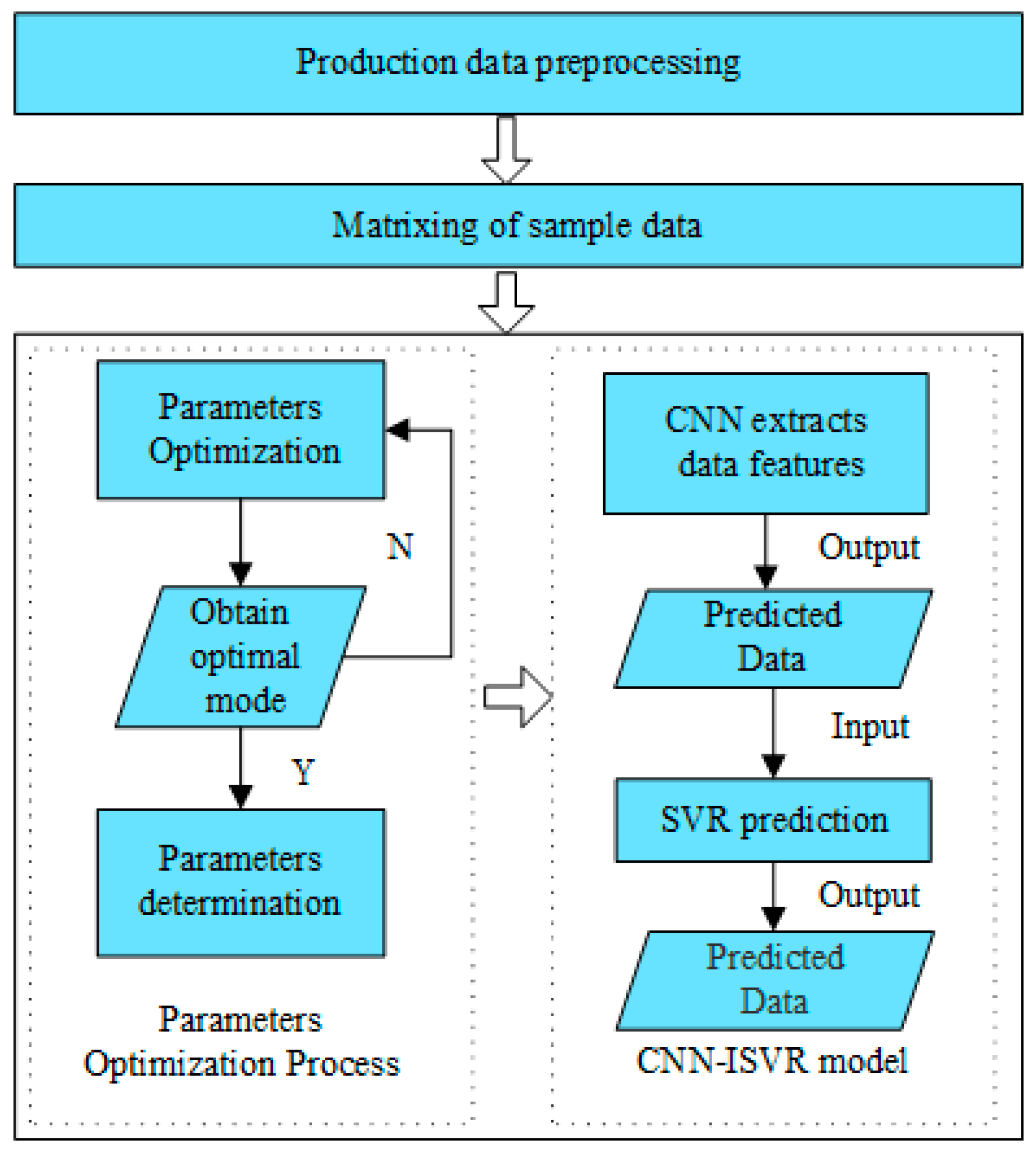
The predicted process flow of the engine production line based on CNN-ISVR is depicted in Figure 2. Initially, actual production line data are obtained and normalized, followed by division of the data into training and testing sets. Concurrently, the ISVR model is subjected to parameter optimization to attain the optimal combination of hyperparameters. Subsequently, a production yield prediction model is established, and the model is trained using the training set. The trained model is then utilized to predict and store the results for the testing set after 10 iterations of training. Finally, the predicted results are output and compared to select the optimal production yield prediction model.

4. Improved GA-SVR Algorithm

Most machine learning algorithms require some level of manual guidance and are not fully automated. The hyperparameters of machine learning algorithms need to be determined in advance through search, optimization, or heuristic techniques. When utilizing the SVR regression model for predicting engine production line yields, it is crucial to incorporate intelligent algorithmic improvements to optimize the key parameters of the SVR model and achieve its optimal performance.
This study primarily focuses on optimizing the penalty parameter  C  and the kernel parameter γ of the RBF. The penalty parameter C signifies the level of punishment for model errors larger than ε in the samples, while the width parameter γ determines the local width of the model and the complexity of its boundaries. In this study, a method is proposed that combines an elite strategy-enhanced GA with a parameter optimization approach based on GS and CV. This combined approach effectively optimizes the parameter selection of the regression prediction model and enhances its prediction accuracy.

4.1. Genetic Algorithm

In GA, the individuals within a population are referred to as chromosomes, representing potential solutions to the problem being addressed. Through the continual evolution of chromosomes, the potential solutions to the problem gradually converge towards the correct solution. The fundamental principles of GA have been extensively documented in earlier literature and numerous books. The improvements in GA primarily encompass encoding schemes, initial populations, fitness functions, and elite selection genetic operators [22,23].
Genetic operators constitute a vital component of GA, comprising selection operators, crossover operators, and mutation operators. The selection operator significantly enhances the convergence speed of the algorithm, while the crossover and mutation operators expand the population diversity, preventing premature convergence of the algorithm.
During the iterative process of GA, the selection operator utilizes the roulette wheel selection algorithm to choose superior individuals from the parent generation for the offspring. The probability of an individual being selected in the offspring population is calculated based on Equation (15), and individuals are chosen accordingly to form the offspring population for the next iteration. The probability of selection increases with higher fitness values of the individuals.
P i = f ( i ) i = 0 n f ( i )
where:  P i  represents the probability of each individual being selected,  f i  denotes the fitness of individual  i , and  n  signifies the population size.
The crossover operator serves as a primary method for generating new individuals and determines the global search capability of the algorithm. During the early stages of evolution within the population, increasing the number of individual crossovers is advisable to accelerate the exploration in the solution space. However, in the later stages of evolution, reducing the number of individual crossovers is necessary to preserve excellent genetic traits. The optimized crossover probability, denoted as  P c , is adaptively defined through the following arithmetic operation.
P c = ( ( L l L P c m a x + l L P c m i n ) + P c m a x f m a x f m i n ) 2
where  L  represents the total number of generations in the evolutionary process, while  l  denotes the current generation of the population.  P c m a x  and  P c m i n  refer to the maximum and minimum values of the crossover probability, respectively. Similarly,  f m i n  and  f m a x  correspond to the minimum and maximum fitness values within the current population.
The mutation operator serves as an auxiliary method for generating offspring in the population, and it determines the local search capability of the GA. As the algorithm iterates and the number of generations increases, the chromosomes in the population gradually approach the optimal solution. In the later stages of evolution, even though the algorithm can explore new spaces through mutation, it is necessary to set the mutation probability to a lower value. This is because a high mutation probability can increase the convergence time of the algorithm and even disrupt the current patterns. The optimized mutation probability is defined as [23].
P m = L l L P m m a x + l L P m m i n
where:  P m m a x  and  P m m i n  represent the maximum and minimum values of the mutation probability, respectively.

4.2. Elite Strategy Genetic Algorithm

In the iterative process of traditional GA, the commonly used strategy for selecting offspring from the parent population is the roulette wheel selection method. This method leads to the loss and disruption of individuals with higher fitness in the parent population, resulting in problems such as premature convergence and limited global optimization effectiveness in the later stages of training.
To address the aforementioned issues and consider the shortcomings of traditional GA during the iterative process, this study proposes the incorporation of an elite strategy selection operator into the traditional GA. This involves preserving and replacing low-fitness individuals in the offspring population with superior individuals from the parent population. These exceptional individuals form an elite population that serves as a backup, ensuring that elite individuals are not lost or disrupted during the evolution process through selection, crossover, and mutation operations.
The top  k  high-performing individuals from each population  P O P i ( i = 1, 2, …,  n )  are preserved in their respective elite populations  E P O P i ( i = 1, 2, …,  n ). Throughout each iterative cycle, it is ensured that each elite population consistently retains the top  k  individuals from their respective population’s developmental process.
By employing the elite selection operator to choose the optimal solution from the current population and performing elite backup, the algorithm iteratively identifies the best solution. This approach effectively prevents the conventional genetic algorithm from being trapped in local optima, enhances convergence speed, and further improves the predictive accuracy of the SVR model.

4.3. Optimization of Hyperparameters for SVR Model

GS is a method for hyperparameter tuning, which involves exhaustively searching all possible parameter combinations within a given range to find the optimal set of hyperparameters that yield the best model performance [24]. CV is a statistical technique used to assess the performance of a classifier, effectively preventing overfitting and underfitting [25].
The two key hyperparameters in the SVR model training process are denoted as ( C γ ). Since their selection does not rely on prior knowledge, combining the aforementioned methods is employed to optimize the hyperparameters of the SVR model. The specific steps for optimization are as follows:
Step 1:
Determine the range of values for the hyperparameters ( C γ ). The commonly used range is [2−10, 210].
Step 2:
Perform GS on the hyperparameters. Since the parameter range spans a wide range, taking the logarithm base 2 of the hyperparameter values gives us  l o g 2 C ,   l o g 2 λ [10, −10]. Using an interval of 0.25, we can obtain a total of 81 × 81 = 6561 hyperparameter combinations.
Step 3:
K -fold CV. Choose 600 samples out of 500 as training data and 100 samples as testing data. Let  K  = 5, then divide the training data into 5 equal parts and use each part in turn as the validation set to evaluate the quality of the model trained by the remaining 4 parts. Finally, select the hyperparameters with the minimum root-mean-square error as the optimal hyperparameters in the CV process.
Step 4:
Hyperparameter combination grid search. Repeat step 3 for the next group of hyperparameter combinations until the combination with the smallest mean squared error is found, which becomes the optimal SVR model hyperparameters for the current sample set. When different parameter combinations ( C ,   γ ) correspond to the same cross-validation accuracy during the model training process, it is generally preferable to choose the combination with smaller  C  to improve the model’s generalization ability.

4.4. Optimization Process of the SVR Model

For this section, the chosen criterion for iteration is the evolutionary generation, which defaults to ending when the evolutionary generation reaches 50. The fitness function is responsible for evaluating the quality of individuals in the population and determining the direction of population evolution. Therefore, the fitness function is critical throughout the entire iteration process. In this article, Mean Squared Error (MSE) is chosen as the fitness function, defined by the following arithmetic operations:
MSE = 1 m i = 1 m ( ( f ( x i ) y i ) ) 2
where  m  represents the number of samples used for training,  y i  stands for real values of the samples, and  f x i  serves as the predicted value of the samples. It is evident that a smaller MSE signifies higher accuracy in the predicted values.
The basic steps for optimizing the parameters of the SVR model in this article are as follows:
  • Determine the optimized parameters and encode them, setting the initial range for the optimization.
  • Generate an initial population by randomly producing individuals and setting relevant parameters to improve the GA.
  • Calculate the fitness using MSE as the evaluation criterion in the sense of the GS-CV algorithm, verifying the classification accuracy.
  • Employ adaptive crossover and mutation techniques, as well as conduct elite selection and backup.
  • Determine the termination condition: if the number of iterations is met or the solution converges, then decode and output the optimal SVR parameter solution; otherwise, repeat step 2 and continue the process.

4.5. Optimization Results of SVR Model Parameters

To obtain the optimal model parameters, it is necessary to predefine the initial parameters and the optimization parameter value range in the genetic algorithm, as well as provide an appropriate number of CV times to ensure the trustworthy optimal solution while avoiding heavy computation. This section first presents the selection of three essential elements for mathematically designing optimized models based on GA optimization of SVR model parameters. The optimally designed mathematical model often takes the form of:
o p t . z = f ( x , y ) x , y D s . t . h i ( x , y ) = 0 ( i = 1 , 2 , 3 n ) g j ( x , y ) 0 ( j = 1 , 2 , 3 n )
where  z  represents the objective function, which in this paper is the minimum value of the cumulative mean squared error generated by the GS-CV method. The functions  h i x , y  and  g j x , y  serve as inequality constraints, both of which are utilized in this study to constrain the GS-CV hyperparameter optimization. Specifically, they require that the MSE produced from a single iteration of optimization be less than 1 × 10⁻⁴ and that the maximum number of iterations falls below a predetermined number. The design variables encompass the penalty parameter C and the amplitude  γ  of the RBF kernel function for the SVR regression model. The variable space and elite strategy genetic algorithm (E-GA) parameters can be found in Table 2:
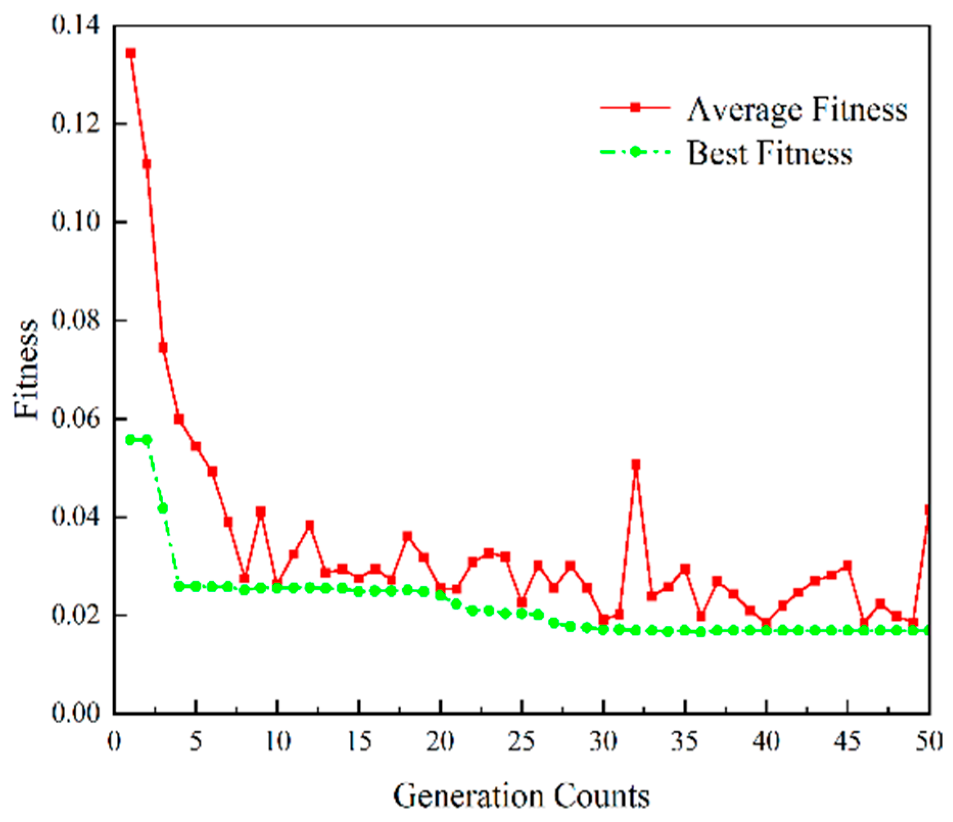
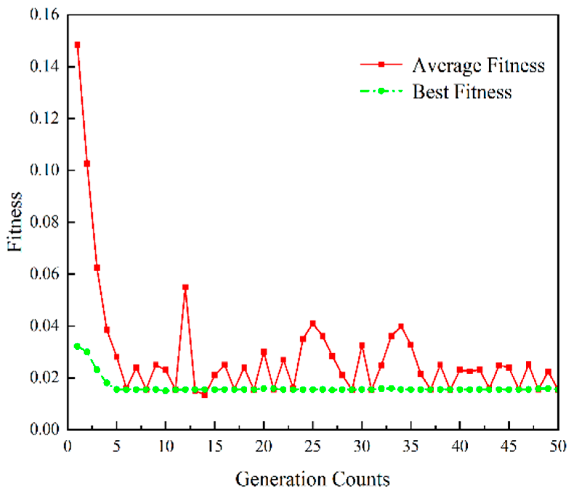
According to the parameter setting method shown in Table 2, the GA-SVR and E-GA-SVR models were subjected to hyperparameter optimization under GS-CV. The fitness variation curves of the  C / γ  search algorithm for optimization were obtained and are shown in Figure 3 and Figure 4, respectively.
Under the GS-CV hyperparameter optimization with  K  = 5, the best penalty factor  C , optimal kernel function width  γ , and MSE values for the two SVR models obtained through GA and improved GA via elitist strategy are presented in Table 3:
Figure 3 and Figure 4 depict the fitness evolution curves of two SVR yield models. Compared to the GA-SVR model, the E-GA-SVR model achieves a stable fitness rate faster within the same number of 50 iterations. After only 4 iterations, it reaches the global optimum value of fitness, with a clear decrease in fitness compared to the GA-SVR model. Therefore, the SVR model that is proposed in this paper, which is based on elite strategy genetic algorithm, improves convergence speed and prediction accuracy relative to the traditional GA-SVR model. Afterwards, the output of the fully connected layer is used as the final extracted feature and input into the improved SVR model to predict engine production line yield.

5. The Production Prediction for Aerospace Engine Production Lines

5.1. The Acquisition of Production Line Data

The acquisition of production data on aerospace engine assembly lines heavily relies on Industrial Communication Protocols (ICPs). ICPs are protocols utilized in industrial environments to connect systems, interfaces, and machinery. They facilitate real-time retrieval of machine monitoring data from the production line, empowering real-time data analysis platforms for tasks such as predictive analytics. However, the effectiveness of these protocols remains largely unknown, and there is a lack of experiential evaluation comparing their performance. Tapia [26] embraced the concept of edge computing and evaluated the performance of ICPs using three different machine tools. From a software perspective, it was found that Modbus provides optimal latency data, offering advanced experiential insight for selecting ICPs in industrial settings.

The Communication between Devices and Modbus TCP

This text discusses the process of extracting data from production equipment on the engine assembly line using the Modbus TCP Python library. When connecting to the production equipment, it is crucial to ensure that it is within the same network range. Next, the device’s IP address and the Modbus TCP port should be specified. After determining the input register addresses and their respective data types provided by the manufacturer, it is necessary to define the address range to ensure the provision of the starting and ending addresses of the registers to be read.
Among the most relevant monitoring variables in the engine production line devices are the device status, production data, and device parameters. The device status enables the monitoring of the device’s operational state and load conditions, such as power on, power off, running, and stopping. Production data allow for the monitoring of data during the production process, such as production quantity, production cycle time, and processing quality. Device parameters enable the monitoring of operational parameters, such as temperature, pressure, current, and voltage.

5.2. Reprocessing of Production Data

The aerospace engine production line studied in this paper is a small sample, non-linear model. In previous research, the applicability of machine learning algorithms has been tested on small datasets, including their instances and inputs [27]. However, these conditions are not common in practical production environments. Additionally, small-scale experimental datasets have been shown to potentially decrease the efficiency of machine learning algorithms or result in some prediction model failures, such as overfitting. If the dataset size increases, most machine learning algorithms will provide better results [28], although they may include noise effects.
Therefore, this paper takes into account the reduction in performance of machine learning models in the case of small sample datasets. Using the method of ensemble learning [29], the size of the dataset is increased through experimental repetition under the same production conditions to achieve higher accuracy of the machine learning models.

5.3. Display of Production Data

The data in this article are derived from the production line of a certain model of aerospace engine. In the actual production line, Modbus TCP is used to collect the production cycle of each device, the load of each device, and the utilization of the devices. The enhanced integration method is employed to repeat experiments under the same production conditions, aiming to increase the size of the dataset. This method replaces the traditional approach of using data averages, thus enhancing the predictive performance of the machine learning model. The first column of the selected data serves as the output indicator for regression prediction, while the remaining columns act as input features, forming the core matrix parameters of the model. Table 4 presents a subset of the production line data collected continuously over a certain period of time.

5.4. Design of Evaluation Metrics

To evaluate the performance of different yield models, this study employs Root Mean square Error (RMSE), Mean Absolute Percentage Error (MAPE), and coefficient of determination (R2) as accuracy measures for prediction results. RMSE compares the deviation between predicted and true values, while MAPE measures the accuracy of a model’s prediction results (R2) is the square of the correlation coefficient, with a value range of (0–1). The larger the value, the higher the degree of explanation of the independent variables for dependent variables, indicating a better fit. The corresponding calculation formulas are shown in Equations (20)–(22).
R 2 = 1 i = 1 M y i y i ^ 2 i = 1 M y i y ¯ 2
RMSE = 1 M i = 1 M y i y ^ i 2
MAPE = 1 M i = 1 M y i y ^ i y i
where  M  represents the number of samples;  y i  represents the actual production of the  i -th set of data;  y ^ i  represents the predicted production of the  i -th set of data;  a n d   y ¯  represents the mean value of the actual production.

5.5. Normalization Process

To enhance the recognition accuracy of the subsequent engine production line capacity prediction model training and to ensure physical significance in the computation, it is necessary to perform normalization on the sample output data in Table 4 before training and predicting the model.
x = x i x m i n x m a x x m i n
where  x m a x  and  x m i n  represents the maximum and minimum values of the input sample  x i , respectively;  a n d   x  refers to the normalized value obtained through processing.

5.6. Experimental Design

The experiment conducted for this study used the Windows 11 operating system. We used PyCharm as our development environment and implemented the experiment using Python 3.6. Throughout this process, we employed TensorFlow 2.0’s Keras deep learning module to construct CNN-ISVR, CNN-SVR, and CNN models. Furthermore, we utilized the scikit-learn library to build an SVR model, employed the DEAP library to construct a genetic algorithm model, and ultimately implemented a genetic algorithm based on elite strategy improvement using the PyGAD library.

5.6.1. The Pre-Processing and Matrixing of Input Data

The simulation-generated first 400 sets of production data are used as the training set for the model, and the following 100 sets of data are used for testing the model. Here is the procedure of the input data pre-processing and matrixing process.
  • The column padding operation is performed on the input production data to enable each sample vector to be matrixed. Five zero vectors are added after the original 220 columns of data, and the size of the data matrix becomes 500 × 225.
  • Normalize the data. Considering the requirements of CNN on data, the data are normalized to [0, 1] according to Formula (20), which eliminates the interference of dimensional disturbance of data while ensuring that the data distribution remains unchanged.
  • Matrixize each row sample vector. Each row sample changes from a 1 × 225 vector form to a 15 × 15 matrix form.
  • Up-sample the data as the input for the CNN model. The corresponding sample matrix of 200 × (15 × 15) is up-sampled to a 4-dimensional matrix of size 500 × 15 × 15 × 1.

5.6.2. Parameters of CNN-ISVR Model

The CNN model architecture is composed of an input layer, two convolutional layers, two fully connected layers, and an output layer. The number of convolutional kernels in the two convolutional layers are, respectively, 32 and 64, with a kernel size of 2 × 2 and a feature size of 8 × 8. The details of the parameters of the CNN model framework are shown in Table 5:
In the SVR model with the RBF kernel, selecting the appropriate penalty parameter  C  and kernel function parameter γ is crucial for prediction accuracy. This article employs a combination of the genetic algorithm with the improved elitist strategy proposed in Section 3 and hyperparameter optimization methods based on GS-CV to optimize the kernel function parameters in CNN-ISVR, obtaining the optimal combination of hyperparameters as shown in Table 3.
To validate the effectiveness and generalizability of the CNN-ISVR production forecasting model, we employed the CNN and SVR algorithms to predict the engine production on the test set. Furthermore, we compared these predictions with those obtained from typical regression algorithms such as Linear Regression (LR), Ridge Regression (RG), and Random Forest (RF).
Regarding the traditional SVR model, this article utilizes the GS method to search for the optimal combination of  C  and γ hyperparameters. The set of possible values for γ includes {0.01, 0.1, 0.25, 0.5, 1}, while the set of possible values for  C  includes {0.001, 0.01, 0.1, 1, 10, 50, 100, 1000}. Due to the susceptibility of grid-search to local optima, the combination parameter that is recorded the most number of times is selected as the experimental parameter. Each group is repeated 10 times in total, and the average prediction results are shown in Table 6. The model performs best when γ is “scale” and  C  is 4, which is why this combination is selected as the optimal model parameter.
The LR model fits the data using the least squares method. Since the data are not centralized, the resulting model does not pass through the origin. Therefore, the model intercept is set to True. Additionally, the data set has been normalized during construction, and normalization is set to False in this case.
The RG regularization coefficient is set to 2, and the model intercept is set to True. Iterations are performed using the Stochastic Average Gradient (SAG) descent method. For the RF, the maximum number of iterations for learning is set to 100, and the evaluation criterion for features is MSE. The parameter settings for each model are presented in Table 7.

5.7. Analysis of Production Line Yield Model Prediction Results

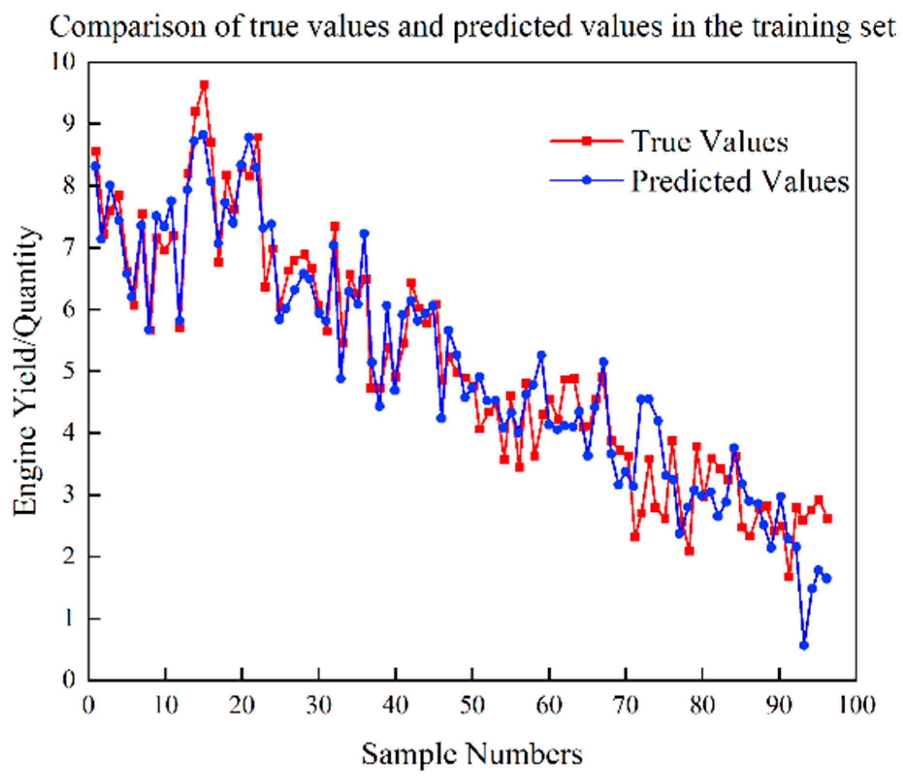
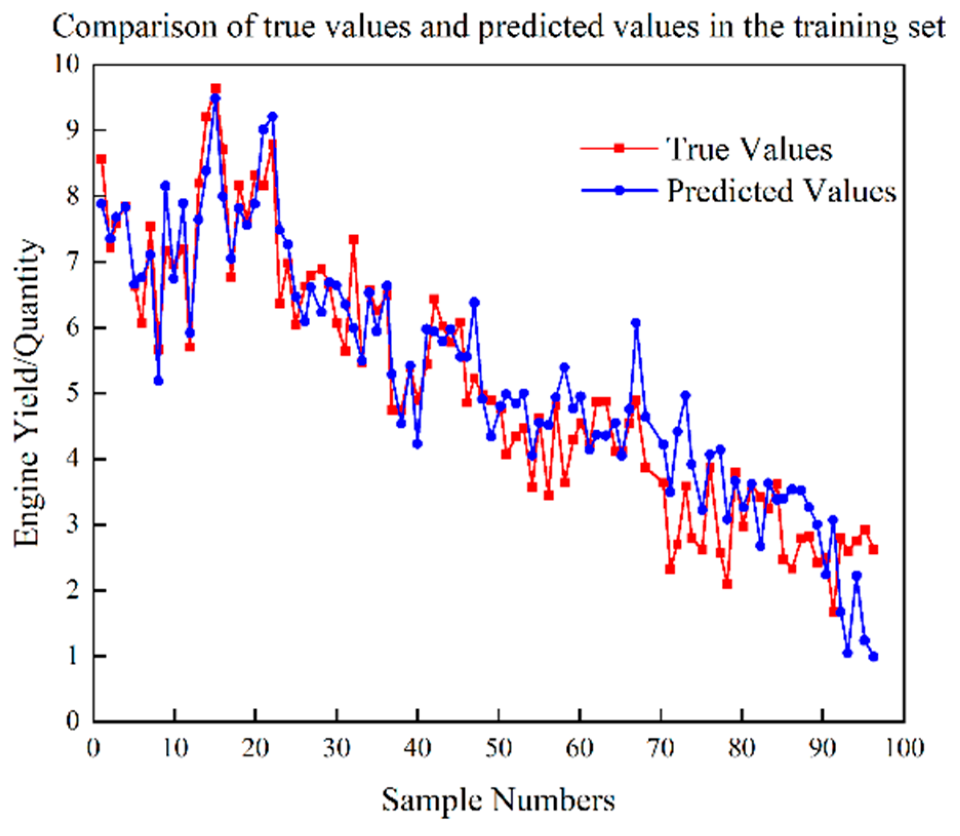
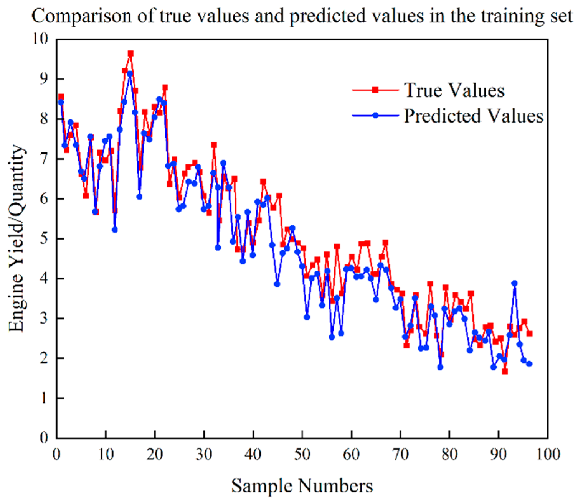
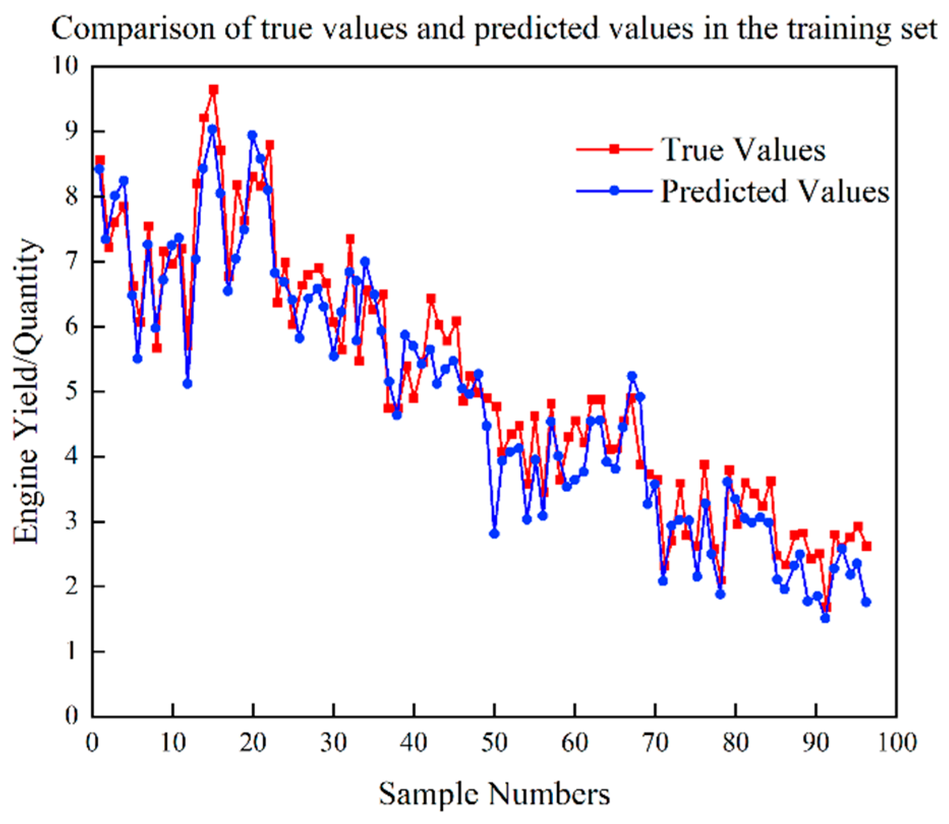
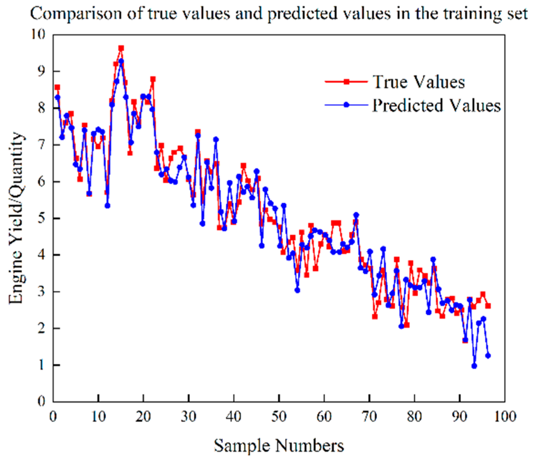
The model training process selected 300 sets of production data from a certain model of engine production line. The first 200 sets of data were used as the training set for the model, and the remaining 100 sets of data were used as the test set for the model. In order to verify the differences between the CNN-ISVR, CNN-SVR, SVR, and CNN yield models established in this study, the yield models of LR, RG, RF, SVR, CNN, CNN-SVR, and CNN-ISVR were trained using the training set. Then, the yield of the engine production line was predicted using each of the yield prediction models. The test set prediction results of each yield prediction model are shown in Figure 5, Figure 6, Figure 7, Figure 8, Figure 9, Figure 10 and Figure 11, and the comparison between the true values and the predicted values of each model is shown in Figure 12.
Based on Figure 5, Figure 6, Figure 7, Figure 8, Figure 9, Figure 10, Figure 11 and Figure 12, it is evident that the proposed CNN-ISVR model exhibits superior predictive performance. Compared to the SVR, CNN, and CNN-SVR models, the CNN-ISVR model demonstrated markedly higher prediction accuracy and better fitting with true values.
To quantify the superior generalization ability of the CNN-ISVR regression model, a comparison of relative errors was conducted for four different methods, namely SVR, CNN, CNN-SVR, and CNN-ISVR, within the same prediction period. The obtained results are presented in Figure 13:
Based on the comparison of the relative errors obtained, the yield prediction results from all four methods appear to be relatively conservative. Due to the fact that the CNN-ISVR model has a large penalty parameter  C , which was optimized through a GA, its punishment power on the erroneous samples is relatively strong. Therefore, most of the predicted values are biased towards the true values. The majority of relative errors are positive, which suggests that, within a certain production period, the predicted yield is higher than the actual yield. In practice, engine manufacturers typically adopt a strategy of optimizing bottleneck workstations, using automated and intelligent equipment to replace manual labor, and enhancing the skills and knowledge of the operators, in order to further improve the overall efficiency of the production line. Therefore, the analysis of the relative error comparison chart indicates that the actual production line conditions and the predicted yield trend are consistent.
Based on the predicted error trend, the proposed CNN-ISVR model in this study demonstrated a significant reduction in variance of relative error compared to the SVR model, CNN model, and CNN-SVR model within the same prediction cycle, with reductions of 84.81%, 92.64%, and 72.65%, respectively. Furthermore, the CNN-ISVR model exhibited a clear decrease in accumulated relative error compared to the SVR model, CNN model, and CNN-SVR model. These findings suggest that using the CNN-ISVR method for prediction results in a more stable overall numerical fluctuation of errors and effectively improves the model’s generalizability.
The accuracy assessment of the prediction results is presented in Table 8:
According to Table 8, the RMSE of the CNN-ISVR model is 2.1428. This represents a reduction of 47.11%, 48.03%, 53.19%, 48.55%, 57.97%, and 40.07% compared to the LR, RG, RF, SVR, CNN, and CNN-SVR models, respectively. Furthermore, the MAPE of the CNN-ISVR model is 4.4758%, indicating a decrease of 32.95%, 45.73%, and 19.95% in comparison to the SVR, CNN, and CNN-SVR models, respectively. These results clearly demonstrate the superior predictive accuracy of the CNN-ISVR regression model.

6. Conclusions

The proposed method presents an innovative approach for predicting the production yield of aerospace engine assembly lines, based on the CNN-ISVR hybrid model.
Considering the machining characteristics of the engine production line, the factors that affect the production yield are determined and quantified from two aspects: production pace and real-time line status, including production pace, equipment load, equipment status, and line operation.
By utilizing the key production process data of the engine assembly line as model input, an adaptive feature extraction is performed using a shallow, non-dimensional reduction CNN. This eliminates the need for feature pre-extraction, effectively overcoming the limitations of support vector regression. The resulting extracted features are then used as input for the improved SVR model, which incorporates an elite strategy genetic algorithm. This enables accurate prediction of the engine production line yield, providing an intuitive reflection of the line’s production capacity.
To validate the effectiveness and generalization of the constructed CNN-ISVR quality prediction model, a comparison is made with other commonly used regression prediction models. The results demonstrate that the CNN-ISVR model exhibits superior fitting performance and smaller prediction errors, enabling accurate and effective prediction of the engine production line yield.
This method proposed in the study offers a practical reference solution for predicting the production yield of aerospace engine assembly lines, assisting enterprises in enhancing production efficiency and optimizing production scheduling. However, further investigation is required to address factors that currently remain unquantifiable or difficult to collect, such as material supply efficiency and operator skill levels. Therefore, future research efforts will be devoted to exploring approaches for acquiring and integrating these production process data, aiming to obtain more accurate predictions that closely align with the actual production line conditions.

Author Contributions

Conceptualization, H.L. and B.L.; methodology, H.L.; training neural networks, B.L.; improvement of regression algorithms, H.L.; collecting and gathering data, C.L. and M.Z.; data curation, M.L.; writing—original draft preparation, H.L.; writing—review and editing, B.L.; visualization, B.L.; supervision, H.L.; project administration, B.L. All authors have read and agreed to the published version of the manuscript.

Funding

The APC was funded by Shenyang Aerospace University, Publication Support Program.

Data Availability Statement

Not applicable.

Conflicts of Interest

The authors declare no conflict of interest.

Nomenclature

Full NameAbbreviations
Support Vector RegressionSVR
Improved Support Vector RegressionISVR
Radial Basis FunctionRBF
Convolutional Neural NetworksCNN
Genetic AlgorithmGA
Grid-SearchGS
Cross-ValidationCV
Radial Basis Kernel FunctionRBF
Mean Squared ErrorMSE
Root Mean Square ErrorRMSE
Mean Absolute Percentage ErrorMAPE
Linear RegressionLR
Ridge RegressionRG
Random ForestRF
Industrial Communication ProtocolsICPs

References

  1. De Leone, R.; Pietrini, M.; Giovannelli, A. Photovoltaic energy production forecast using support vector regression. J. Neural Comput. Appl. 2015, 26, 1955–1962. [Google Scholar] [CrossRef]
  2. Li, D.; Wang, L.; Huang, Q. A case study of SOS-SVR model for PCB throughput estimation in SMT production lines. In Proceedings of the IEEE International Conference on Industrial Engineering and Systems Management (IESM), Shanghai, China, 25–27 September 2019; pp. 1–6. [Google Scholar]
  3. Hu, X.R. Simulation Study of Fully Automatic Cotton Yarn Dyeing and Printing Production Line Based on Unity3D; Donghua University: Shanghai, China, 2020. (In Chinese) [Google Scholar]
  4. Gaonkar, B.; Davatzikos, C. Analytic estimation of statistical significance maps for support vector machine based multi-variate image analysis and classification. J. Neuroimage 2013, 78, 270–283. [Google Scholar] [CrossRef]
  5. Nandi, S.; Badhe, Y.; Lonari, J. Hybrid process modeling and optimization strategies integrating neural networks/support vector regression and genetic algorithms: Study of benzene isopropylation on Hbeta catalyst. J. Chem. Eng. J. 2004, 97, 115–129. [Google Scholar] [CrossRef]
  6. Han, Y.; Liu, Y.; Pan, Y.H. Comparison of SVM, BP neural network and linear regression. J. North China Univ. Sci. Technol. 2017, 39, 104–109. [Google Scholar]
  7. Zhang, J.; Wang, J.; Qin, W.; Rosa, J.L.G. Artificial neural networks in production scheduling and yield prediction of semiconductor wafer fabrication system. In Artificial Neural Networks-Models and Applications; IntechOpen: London, UK, 2016; pp. 355–387. [Google Scholar]
  8. Nuñez-Piña, F.; Medina-Marin, J.; Seck-Tuoh-Mora, J.C. Modeling of throughput in production lines using response surface methodology and artificial neural networks. J. Complex. 2018, 1–10. [Google Scholar] [CrossRef]
  9. Yang, Y.Y.; Liu, G.L.; Zhao, G.H. A long shortterm memory based deep learning method for industrial load forecasting. J. Power Constr. 2018, 39, 29–36. (In Chinese) [Google Scholar]
  10. Ye, Y.W.; Lu, J.J.; Qian, Z.Q. Study on the Temperature Error Prediction of Mechanical Temperature Instrument Based on LSSVM. J. Chin. J. Sci. Instrum. 2016, 37, 57–66. (In Chinese) [Google Scholar]
  11. Zhang, L.; Zhou, W.D.; Chang, P.C. Iterated Time Series Prediction with Multiple Support Vector Regression Models. J. Neurocomputing 2013, 99, 411–422. [Google Scholar] [CrossRef]
  12. Tang, Y. Deep learning using linear support vector machines. arXiv 2013, arXiv:1306.0239. [Google Scholar]
  13. Shi, Y.G.; Cheng, K.; Liu, Z.W. Hippocampus sub-area image segmentation combined with deep learning and support vector machine. J. Image Graph. 2018, 23, 542–551. (In Chinese) [Google Scholar]
  14. Shi, P.M.; Liang, K.; Zhao, N. Gear intelligent fault diagnosis based on deep learning feature extraction and particle swarm support vector machine state recognition. J. China Mech. Eng. 2017, 28, 1056–1061. (In Chinese) [Google Scholar]
  15. Kang, Z.; Catal, C.; Tekinerdogan, B. Machine learning applications in production lines: A systematic literature review. J. Comput. Ind. Eng. 2020, 149, 106773. [Google Scholar] [CrossRef]
  16. Chang, L.; Deng, X.M.; Zhou, M.Q. Convolutional neural networks in image understanding. J. Acta Autom. Sin. 2016, 42, 1300–1312. (In Chinese) [Google Scholar]
  17. Zhou, F.Y.; Jin, L.P.; Dong, J. Review of convolutional neural networks. J. Comput. 2017, 40, 1229–1251. (In Chinese) [Google Scholar]
  18. Zhang, W.D.; Xu, Y.L.; Ni, J.C. Image target recognition algorithm based on multi-scale block convolutional neural network. J. Comput. Appl. 2016, 36, 1033–1038. (In Chinese) [Google Scholar]
  19. Yang, Y.; Wang, Z.Q.; Yang, B. A predictive model for fixture layout optimization of aerospace thin-walled parts based on support vector regression. J. Comput. Integr. Manuf. 2017, 23, 1302–1309. (In Chinese) [Google Scholar]
  20. Boser, B.E.; Guyon, I.M.; Vapnik, V.N. A training algorithm for optimal margin classifiers. In Proceedings of the Fifth Annual Workshop on Computational Learning Theory, Pittsburgh, PA, USA, 27–29 July 1992; pp. 144–152. [Google Scholar]
  21. Kingma, D.P.; Ba, J. Adam: A method for stochastic optimization. arXiv 2014, arXiv:1412.6980. [Google Scholar]
  22. Huang, J.; Bo, Y.; Wang, H. Electromechanical equipment state forecasting based on genetic algorithm–support vector regression. J. Expert Syst. Appl. 2011, 38, 8399–8402. [Google Scholar] [CrossRef]
  23. Tao, P.Y.; Sun, Z.; Sun, Z.X. An improved intrusion detection algorithm based on GA and SVM. J. IEEE Access 2018, 6, 13624–13631. [Google Scholar] [CrossRef]
  24. Bergstra, J.; Bengio, Y. Random search for hyper-parameter optimization. J. Mach. Learn. Res. 2012, 13, 281–305. [Google Scholar]
  25. Smola, A.J.; Schölkopf, B. A tutorial on support vector regression. J. Stat. Comput. 2004, 14, 199–222. [Google Scholar] [CrossRef]
  26. Tapia, E.; Sastoque-Pinilla, L.; Lopez-Novoa, U. Assessing Industrial Communication Protocols to Bridge the Gap between Machine Tools and Software Monitoring. J. Sens. 2023, 23, 5694. [Google Scholar] [CrossRef] [PubMed]
  27. Bustillo, A.; Pimenov, D.Y.; Matuszewski, M. Using artificial intelligence models for the prediction of surface wear based on surface isotropy levels. J. Robot. Comput. Integr. Manuf. 2018, 53, 215–227. [Google Scholar] [CrossRef]
  28. Grzenda, M.; Bustillo, A. The evolutionary development of roughness prediction models. J. Appl. Soft Comput. 2013, 13, 2913–2922. [Google Scholar] [CrossRef]
  29. Bustillo, A.; Reis, R.; Machado, A.R. Improving the accuracy of machine-learning models with data from machine test repetitions. J. Intell. Manuf. 2022, 33, 203–221. [Google Scholar] [CrossRef]
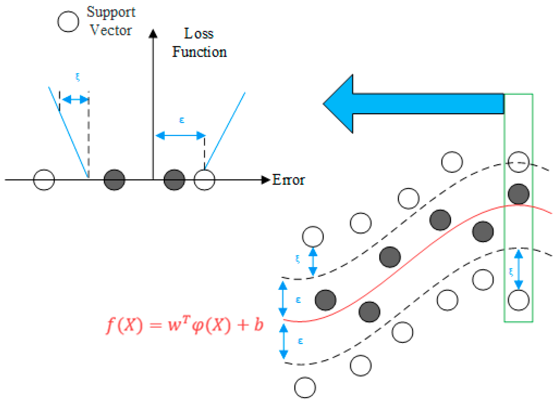
Figure 1. SVR basic principle.
Machines 11 00875 g001
Figure 2. CNN-ISVR-based yield model prediction process.
Machines 11 00875 g002
Figure 3. Fitness evolution curve of parameters in GA-SVR model.
Machines 11 00875 g003
Figure 4. Fitness evolution curve of parameters in E-GA-SVR model.
Machines 11 00875 g004
Figure 5. Test set prediction results of SVR yield model.
Machines 11 00875 g005
Figure 6. Test set prediction results of CNN yield model.
Machines 11 00875 g006
Figure 7. Test set prediction results of LR yield model.
Machines 11 00875 g007
Figure 8. Test set prediction results of RG yield model.
Machines 11 00875 g008
Figure 9. Test set prediction results of RF yield model.
Machines 11 00875 g009
Figure 10. Test set prediction results of CNN-SVR yield.
Machines 11 00875 g010
Figure 11. Test set prediction results of CNN-ISVR yield.
Machines 11 00875 g011
Figure 12. Comparison between true value and predicted values.
Machines 11 00875 g012
Figure 13. Relative error comparison chart.
Machines 11 00875 g013
Table 1. Factors affecting production line yield.
Influencing
Factors
Symbolic
Representation
Descriptions
Production cycle   p 1 , p 2 p n p i  represents the time required to complete the  i th process
Equipment load   q 11 , q 12 q n m q i j  represents the number of the  i th workpiece to be processed on the  j th machine at moment  t
Equipment
condition
  r 1 , r 2 r m
  z
r j  represents the average utilization of the  j th device at time  t  and  z  represents the failure rate of the device at time  t
Production line work system   h h  represents the operating time of the production line for the day
Table 2. Parameter settings for elite strategy genetic algorithm.
Relevant ParametersTake Values (Range)
Maximum number of evolution generations50
Population size20
Range of values for  C  [2−10, 210]
Number of folds for CV ( K )5
Range of values for ( γ )[2−10, 210]
Probability of crossover[0.5, 0.7]
Probability of mutation[0.01, 0.05]
Elite selection operator0.025
Table 3. Optimal hyperparameters combination.
HyperparametersGA-SVRE-GA-SVR
Penalty parameter  C  97.934122.418
kernel function  γ 0.69530.7884
MSE9.35 × 10−5 9.12 × 10⁻⁵
Table 4. Production line data for a certain model of aerospace engine.
Serial NumberEngine Yield
/Unit
Production Cycle p1/HourProduction Cycle p2/HourFacility Load
q11/Unit
Facility Load
q12/Unit
Facility Utilization
r1/%
Facility Utilization
r2/%
Facility Failure Rate z/%Work
System/Hour
1.86.976.000181.5085.4211.18
2.76.995.91081.1384.5810.58
59957.156.080170.4160.4911.88
60047.166.231059.1358.1212.868
Table 5. CNN framework parameters.
Layer StructureFeature SizeFeature ChannelConvolutional Kernel
Input layer8 × 81-
Convolutional layer8 × 8322 × 2
Convolutional layer8 × 8642 × 2
Fully connected layer1 × 51214096 × 1
Output layer1--
Table 6. Average prediction results for different parameter combinations.
  C γR2MAPERMSE
50.60.91586.8716%4.3879
80.60.91886.9654%4.4247
40.80.91676.8921%4.4549
4scale0.92656.6756%4.1651
Table 7. Parameters of other regression models.
ModelParameter Configuration
SVR C  = 4, γ = ‘scale’,  k ( x i , x j )  = ‘RBF’
LRfit_intercept = True, normalize = False, copy_X = True
RGalpha = 2.0, fit_intercept = True, solver = ‘sag’
RFn_estimators = 100, criterion = ‘MSE’, max_features = auto’
Table 8. Comparison of prediction results.
ModelR2RMSEMAPE
LR0.90884.05176.4354
RG0.91224.12356.3290
RF0.90754.57756.8126
CNN0.91835.09828.2477
SVR0.91164.16516.6756
CNN-SVR0.92413.57595.5916
CNN-ISVR0.92652.14284.4758
Disclaimer/Publisher’s Note: The statements, opinions and data contained in all publications are solely those of the individual author(s) and contributor(s) and not of MDPI and/or the editor(s). MDPI and/or the editor(s) disclaim responsibility for any injury to people or property resulting from any ideas, methods, instructions or products referred to in the content.