Article

Synchronous PD Control Using a Time Delay Estimator for a Four-Degree-of-Freedom Parallel Robot in Practice

Automatic Control Department, Ho Chi Minh City University of Technology and Education, Ho Chi Minh 700000, Vietnam
*
Author to whom correspondence should be addressed.
Machines 2023, 11(8), 831; https://doi.org/10.3390/machines11080831
Submission received: 6 July 2023 / Revised: 6 August 2023 / Accepted: 11 August 2023 / Published: 15 August 2023
(This article belongs to the Section Automation and Control Systems)

Abstract

:
This paper presents a synchronous proportional derivative (PD) control method using a time delay estimator (SPD-TDE) for a four-degree-of-freedom (DOF) parallel robot in practice. The proposed control is a method that is developed from a synchronous PD control method combined with a time delay estimator to guarantee the tracking objectives and synchronous requirements of the robot. Firstly, the synchronous PD control method is designed by defining cross-coupling errors. A cross-coupling error is determined by incorporating the tracking error and deviation of tracking error among two adjacent joints or synchronous errors. Then, the asynchronous problem between the kinematic chains is solved and guarantees that the goal of synchronicity is achieved. Consequently, to improve the tracking performance of the robot, a time delay estimator is used to estimate and eliminate the uncertainty components of the system, such as modeling errors and actuator faults. In addition, the Lyapunov theory is also used to demonstrate the stability and robustness of the proposed control method. Finally, a testbench 4-DOF parallel robot is built, and the controllers are embedded in the control board from MATLAB Simulink using the Waijung block set library to operate the robot preset trajectory tracking. The experimental results of the proposed control method for the 4-DOF parallel robot are compared with those obtained using other controllers to prove its effectiveness.

1. Introduction

Nowadays, robots are applied in many fields to replace humans in performing different tasks and to improve production productivity as well as product quality. There are many types of robots that have been researched, developed, and commercialized, and one of them is the parallel robot. The parallel robot has a closed-loop structure; the fixed base is linked to a moving platform with parallel and identical kinematic chains. It has been widely applied in many fields, such as industry [1,2,3], agriculture [4], medicine [5], and motion simulation [6], due to its distinct advantages of high stiffness, high speed, high accuracy, high flexibility, and large load-carrying capacity [7]. However, the closed-loop structure of the robot also brings many difficulties in controlling it, such as a limited workspace, singularity, the forward kinematic problem, and a complicated dynamic model. Many control methods have been proposed to deal with the above problems. And these methods have been divided into two distinct approaches [8]: control methods not based on a model, such as proportional–integral–derivative (PID) control [9,10], fuzzy control [11], and neural network control (NNC) [12]; and model-based control methods such as sliding-mode control (SMC) [13,14], fault-tolerant control (FTC) [15], and adaptive control [16].
Generally, the two control approaches mentioned above solve some problems in parallel manipulator trajectory tracking control. However, an important problem that exists in conventional controllers for parallel robots is that the controllers can only individually control each joint of the robot without feedback from other joints. Meanwhile, the parallel manipulator has a closed-loop mechanical structure, and the moving platform follows the trajectory depending on the coordination of the same kinematic sequences. At any time, a disturbance or transmission error can occur in one of the loops while the others do not respond. The lack of synchronicity between the control loops can lead to uncovered deformation; even deconstruction can happen [17]. To solve this problem, a cross-coupling synchronous control method has been proposed for closed-loop systems.
The cross-coupling control for the serial manipulator was first introduced by Koren [18]. This control method involves defining the tracking error, synchronous error, and cross-coupling error. The deviation between the joint angle response and the reference joint is the tracking error. The difference between the tracking errors of two transmission joints adjacent is the synchronous error. And the combination of tracking and synchronous errors is a cross-coupling error. The cross-coupling error is used to design the synchronous controller and to achieve the goal of synchronicity or the simultaneous convergence of tracking and synchronous errors to zero. As a result, this method significantly improves the tracking performance and ensures the goal of synchronizing the system. Recently, several studies on synchronous algorithms have been published and applied to many subjects. For example, Dong Sun et al. used cross-coupling control technology on CNC machines [19] and multiple-motion-axis systems [20,21,22]. In robotics, Dong Sun et al. designed a synchronous tracking control method for a 3-DOF parallel robot [23]; Weiwei Shang et al. implemented a synchronous method for a planar parallel robot with a redundant actuator in the task space [24]; Piotrr Wos and Ryszard studied a 3-DOF hydraulic translational parallel manipulator [25]; Keke Shi et al. used coupled orbit–attitude dynamics and trajectory tracking control for spacecraft electromagnetic docking [26]; and D. T. Tran et al. experimented with a synchronous algorithm on a 4-DOF parallel manipulator in practice [27]. Considering the above analyses, this study proposes a synchronous proportional derivative (SPD) control method for a 4-DOF parallel robot to solve the asynchronous problem among the joints as well as to guarantee the goal of synchronizing the system. Nevertheless, a 4-DOF parallel robot has high nonlinearity and is always affected by external disturbance and uncertainty components such as modeling error, actuator faults, etc. Meanwhile, the SPD control method has a simple structure without a clearly dynamic model system. So, achieving a high orbital tracking performance and resistance to external disturbance and uncertainty components is a challenge.
Recently, researchers have applied intelligent methods to handle the above problems. Intelligent methods are used to estimate and eliminate external disturbances and uncertainty terms via their integration with linear/nonlinear controllers. For example, in [28], Jinglei et al. designed an adaptive fuzzy backstepping control method based on dynamic surface control for an uncertain robotic manipulator. Fuzzy networks were used to approximate the uncertain modeling error and external disturbance in the system. The control performance of the robotic manipulator was improved significantly. In [29], Chuang Liu et al. proposed an active disturbance rejection control (ADRC) method for the electromagnetic docking of spacecraft in the presence of time-varying delay, fault signals, external disturbances, and elliptical eccentricity. An ADRC scheme was developed to guarantee the relative position, relative velocity, and the estimation errors of relative motion information and the total disturbance of the system. As a result, the proposed control method for the spacecraft achieved high accuracy and strong robustness. However, these intelligent methods require complex computation. So, it is not practical to implement them in real applications. Compared to fuzzy logic or neural networks or ADRC, a well-known technique is the time delay estimator (TDE), which is also used to estimate and cancel nonlinear dynamics. Furthermore, TDE has a simple structure that does not use a dynamic model of the system. Therefore, it is combined with many other control methods to increase the accuracy and improve the performance of the system, such as the combination of a TDE and supervising switching control to synchronous control for a chaos system [30]. A PUMA robot manipulator achieved good tracking performance and chattering reduction using the TDE and fuzzy logics systems [31] and linked to the adaptive PID-fractional-order nonsingular terminal sliding mode control and TDE to obtain higher accurate results for cable-driven manipulators [32]. Other research incorporates the synchronous sliding mode control and TDE to ensure the asymptotic convergence of the errors and eliminate the uncertainty influence of a 2-DOF parallel manipulator [33,34]. To the best of the authors’ knowledge, some studies use the TDE method to control the parallel manipulators. For a 4-DOF parallel robot, due to the complexities of both computation kinematic and dynamic models, there are very few experimental results of this method.
Based on the above analysis, this paper proposed an SPD-TDE control method for a 4-DOF parallel robot in the presence of uncertainties such as modeling errors and actuator faults. The proposed control is designed by combining the PD control, cross-coupling synchronous control, and time-delay estimator. As a result, the asynchronous problem among the chain kinematics is solved, and the nonlinear components in the system are estimated and eliminated in the control process. From that, the quality of trajectory tracking improves significantly, as well as the synchronous objective of the closed-loop system is achieved.
The main contribution of this paper is summarized as follows:
  • The kinematics and dynamics of a 4-DOF parallel robot are presented based on the geometric and Euler–Lagrange methods with the daresay. Next, a synchronous PD control method is designed to solve the asynchronous among the kinematic chains in the closed-loop system. A combination of the SPD control and time delay estimator is formed to estimate the total lumped uncertainty components in the system. So, the quality of trajectory tracking of the robot improved significantly.
  • The stability and robustness of the proposed control are proven using the Lyapunov theory. Furthermore, a testbench 4-DOF parallel is built, and the controllers are programmed in MATLAB Simulink and are embedded in board control to operate robot preset trajectory tracking. From that, the experiment results are collected and evaluated to demonstrate the effectiveness of the proposed control compared to other controllers.
This paper is organized as follows: Section 2 presents the problem formulations. Section 3 presents the design of the proposed control, and the stability analysis of the proposed controller is discussed. In Section 4, the effectiveness of the proposed controller will be demonstrated using the experiment, and the experiment results will be compared to the PD control and the SPD control. Finally, some conclusions and future works are presented.
2. Problem Formulations

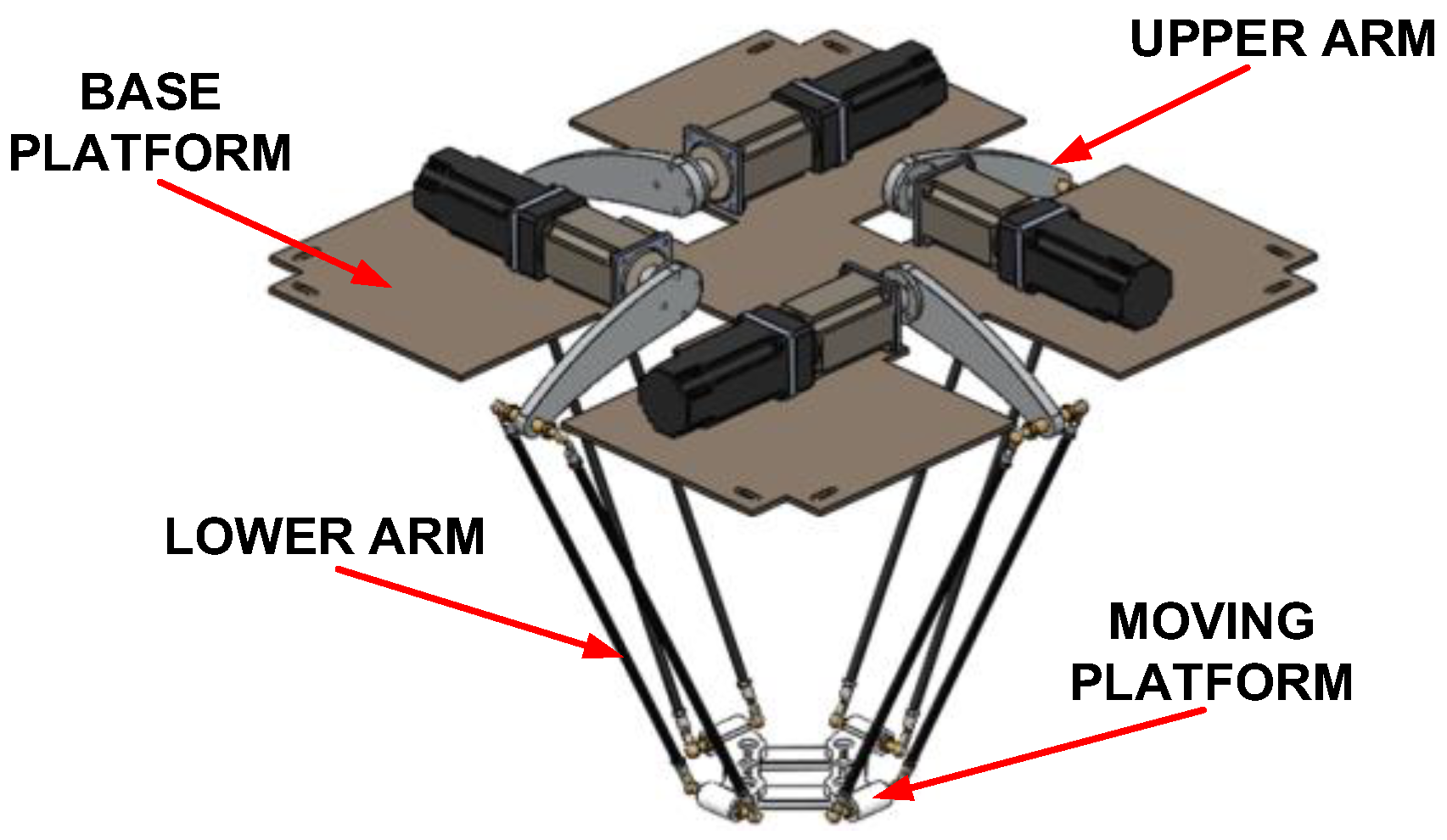
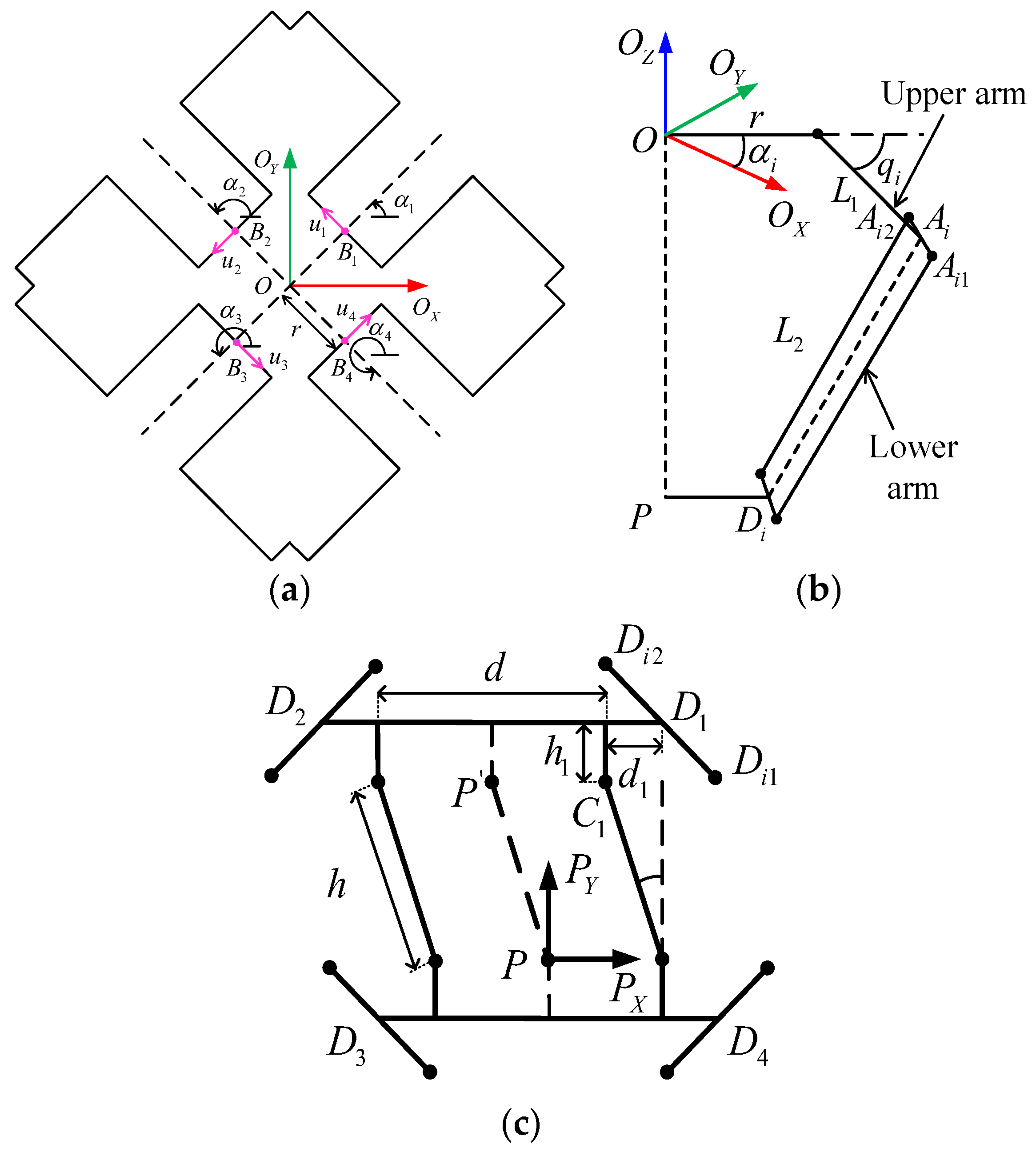
In this section, the solution of the inverse kinematics, forward kinematics, dynamics model, and synchronous method for a 4-DOF parallel manipulator is presented. This model is designed using Solidworks 2021. The model is composed of a base platform or fixed base, a moving platform connected by four upper arms and four lower arms, forming a closed-loop structure characterized by parallel robots, as shown in Figure 1. The physical parameters used in the calculation are extracted from the 3D model of the robot, as shown in Figure 2 and Table 1.

2.1. Kinematics

2.1.1. Inverse Kinematic

In this section, the inverse kinematic solution of a 4-DOF parallel robot determined based on the position end-effector is presented. The origin coordinate system of the robot is set on the base platform, with O is the base platform center, and α i i = 1 , 2 , 3 , 4 is the deviation angle at each upper arm relative to the X axis, as shown in Figure 2a, α i = 2 i 1 π / 4 . The geometric structure of a kinematic chain is shown in Figure 2b, where r is the distance from the origin O to the upper arm revolute joint center O B i = r . L 1 and L 2 are the lengths of the upper arm and lower arm, respectively, B i A i = L 1 , A i D i = L 2 , i = 1 , 2 , 3 , 4 . q i i = 1 , 2 , 3 , 4 is the rotation angle of each upper arm. Figure 2c presents the geometric structure of the moving platform described using x , y , z , θ . Inside x , y , z is the position value of the end-effector in the P X Y Z coordinate system relative to the OX Y Z origin coordinate system, and θ is the rotation angle of the moving platform. In Figure 2c, the coordinate local P X Y Z is present, where P is the controller point, and d , d i , h , h i i = 1 , 2 , 3 , 4 are the geometry parameters of the moving platform. d is the length of the moving platform (along the x-axis). h is the length of the parallelogram bars. h i and d i are the distances between C i and D i , respectively, along the x-axis and y-axis. D i is the midpoint of D i 1 , D i 2 , where the two ball hinges connecting the i t h lower arm with the moving platform.
The kinematic relationship is based on the following equation:
A i D i = L 2
Based on the coordinate O X Y Z system, the coordinates of the points A i , D i and B i is determined.
Equation (1) can be rewritten as follows:
E i sin q i + F i cos q i + G i = 0
where E i , F i , and G i are the functions of the robot geometry.
The inverse kinematic can be obtained by solving Equation (2) as follows:
q i = 2 tan 1 E i E i 2 + F i 2 G i 2 G i F i i = 1 , 2 , 3 , 4
Remark 1.
The formula of E i , F i , and G i functions is presented in detail in Appendix A.

2.1.2. Forward Kinematic

The forward kinematic of a 4-DOF parallel robot aims at calculating the end-effector position by knowing the joint angles q . However, this leads to an eighth-order polynomial in θ . Therefore, the Jacobian scheme can solve the problem more efficiently than the algebraic method.
The Jacobian matrix is the relationship between the end-effector velocities and rotation angle velocities. It can be written as follows:
P ˙ = J q ˙
where J is the Jacobian matrix of the system, P ˙ = X ˙ Y ˙ Z ˙ θ ˙ T is the velocity of the end position of the end-effector, and q ˙ = q ˙ 1 q ˙ 2 q ˙ 3 q ˙ 4 T is the velocity of the rotation angle.
The square on both sides of Equation (1), we can obtain the following:
A i D i 2 = L 2 2
The derivative of Equation (5) for time is given using the following:
A P ˙ + B q ˙ = 0
From Equations (4) and (6), we can obtain the following:
J = A 1 B
The forward kinematic of the parallel robot is obtained via the integration of the below equation as follows [35,36]:
χ n + 1 = χ n + ρ J χ n , q n q d q n
where χ n is the coordinate of the end-effector position, χ n + 1 is the coordinate of the next end-effector position, q n is the current joint angle of the robot, q d is the desired joint angle, and ρ is the arithmetic coefficient.

2.2. Dynamic Model

The dynamic equation of a 4-DOF parallel robot is as follows:
M q q ¨ + C q , q ˙ q ˙ + G q + τ f q , q ˙ + J T F e x t = α τ
where M q R 4 × 4 is the inertial matrix, C q , q ˙ R 4 × 4 is the Coriolis/Centrifugal matrix, G q R 4 × 1 is the gravitational vector, τ f R 4 × 1 is the friction vector, J is the Jacobian matrix, F e x t R 4 × 1 is the external disturbance vector, q , q ˙ , q ¨ R 4 × 1 are the vectors of the position, velocity, and acceleration of the joint angles, τ R 4 × 1 is the joint torques vector, and α R 4 × 4 is the diagonal positive define matrix.
By giving a constant diagonal matrix, M ¯ R 4 × 4 , the expression (9) can be rewritten in another form as follows:
M ¯ q ¨ + N q , q ˙ , q ¨ = τ
where N q , q ˙ , q ¨ = M q M ¯ q ¨ + C q , q ˙ q ˙ + G q + τ f + J T F e x t + I α τ is the total lumped uncertainty components.
Assumption 1.
The connection between the fixed base and the moving platform of the robot is through the links and spherical joints. The mechanical parts are machined with high precision. So, the friction among the joints of the robot is negligible.

2.3. Synchronous Errors and Cross-Coupling Errors

To consider the synchronous of a close-loop chain manipulator, the synchronous control objective is to simultaneously converge both the tracking error e t and synchronous error e s t to zero, whereby the deviation among two adjacent joints is called the synchronous error. Moreover, to achieve this goal, the cross-coupled error is defined as the combination of both tracking and synchronous error, and the cross-coupled error is used to design a synchronous controller.
The synchronous error has the following form:
e s 1 t = e 1 t e 2 t e s 2 t = e 2 t e 3 t e s 3 t = e 3 t e 4 t e s 4 t = e 4 t e 1 t
where e s i t is the synchronous error of the i t h axis, and e i t is the tracking error of the i t h joint.
Equation (11) can be rewritten in the matrix format as follows:
e s 1 t e s 2 t e s 3 t e s 4 t = 1 1 0 0 0 1 1 0 0 0 1 1 1 0 0 1 e 1 t e 2 t e 3 t e 4 t = T e t
The cross-coupled error is expressed below as follows:
E t = e t + β e s t
where E t R 4 × 1 is a cross-coupled error, and β R 4 × 4 is a diagonal matrix positive definite. Substituting (12) into (13), we can obtain Equation (13) in simple form as follows:
E t = I + β T e t
where I is an identity matrix.
Remark 2.
Based on Equation (14), if the inverse I + β T exists, and β is chosen suitable, I + β T , it will be positive definite and have a full rank. When E t 0 leading to e t 0 and e s t 0 , the synchronous control object will be obtained.
The first derivative of the function E t is calculated as follows:
E ˙ t = I + β T t e ˙ t
The second derivative of the function E t is calculated as follows:
E ¨ t = I + β T e ¨ t

3. Control Design

3.1. Synchronous PD Control

The structure of the synchronous PD control for a 4-DOF parallel manipulator under the existence of the uncertainty components is shown in Figure 3. The cross-coupling error receives an informal tracking error of each joint and calculates the synchronous error between two adjacent joints. After that, these two errors are incorporated into the cross-coupling error, which is an input to the controller to calculate the control value.
The control law is presented as follows:
τ = K P 2 E + K D 2 E ˙
where K P 2 , K D 2 R 4 × 4 denote the coefficient matrix of the proportional, derivative terms, respectively, and positive definite. E R 4 × 1 is the cross-coupling error vector.

3.2. Proposed Control

The diagram of the proposed control for a 4-DOF parallel robot in practice is presented in Figure 4. The proposed control is developed from the synchronous PD control based on a time-delay estimator (TDE). The TDE uses the past observation of the response of the system and the control actions rather than adjusting the controller gains or identifying system parameters, thereby leading to a model-independent controller. Indeed, TDE can estimate and eliminate the uncertainty terms such as modeling errors and actuator faults in the system. Therefore, the quality trajectory tracking is improved significantly, and the synchronous of the system is also achieved.
The control objective is the output response q of the system following the reference trajectory q d , which means the tracking error e = q d q converges to zero. The following defines the desired error dynamics:
e ¨ + K D * e ˙ + K P * e = 0
Based on Figure 4, we can see that the control input has the following form:
τ = M ¯ u + N ^ q , q ˙ , q ¨
with
u = q ¨ d + K D * E ˙ + K P * E
where N ^ q , q ˙ , q ¨ denotes the estimate of N q , q ˙ , q ¨ , which is obtained via the TDE subsystem. If the matrix M ¯ is chosen suitable, and the time delay L is small enough, we can obtain N ^ q , q ˙ , q ¨ equal to a slightly time-delayed past value, N q , q ˙ , q ¨ t L , namely as follows:
N ^ q , q ˙ , q ¨ = N q , q ˙ , q ¨ t L
Based on Equation (10), which can find N q , q ˙ , q ¨ at the time t L , and substituting it into Equation (21), we obtain the following:
N ^ q , q ˙ , q ¨ = N q , q ˙ , q ¨ t L = τ t L M ¯ q ¨ t L
From Equations (19), (20) and (22), the SPD-TDE control law for a 4-DOF parallel manipulator is expressed as follows:
τ = M ¯ q ¨ d + K D * E ˙ + K P * E Injecting     desired     dynamics + τ t L M ¯ q ¨ t L TDE
The closed-loop dynamics are produced by replacing Equations (22) and (23) with robot dynamics (10):
e ¨ + K D * E ˙ + K P * E = M ¯ 1 N q , q ˙ , q ¨ N q , q ˙ , q ¨ t L
If the identity of N = N t L is assumed, the closed loop Equation (18) is the desired error dynamics. The stability condition for the TDE is established by Hsia and Gao [37], expressed using the following:
I M 1 M ¯ < 1
When the close loop system is stable using the stability criterion (25), N N t L is bounded because N is the sum of continuous terms and bounded discontinuous terms. The bounded TDE error ε is defined as follows:
ε M ¯ 1 N N t L
Then, the closed-loop system dynamics with the TDE becomes the following:
e ¨ + K D * E ˙ + K P * E = ε
The TDE error ε is close to 0 in most of the operating time of the robot manipulators; however, it exhibits a pulse-type error due to the discontinuity of Coulomb friction at velocity reversal.

3.3. Stability Analysis

The boundedness of ε can be proved in the same manner as the stability proof in [31].
The desired error dynamics can be described in different forms based on (20) and (27) as follows:
ε = u q ¨
Equation (29) is calculated by multiplying (28) with M and combined with Equation (9) as follows:
M ε = M u q ¨ = M u + C q ˙ + G + τ f τ = M u + C q ˙ + G + τ f M ¯ u N t L
Referring to Equation (10), the time-delayed nonlinear component L can be presented as follows:
N t L = M t L M ¯ q ¨ t L + C q ˙ t L + G t L + τ f t L + J T F e x t t L + I α τ t L
Substituting (30) into (29), we have the following:
M ε = M M ¯ u M t L M ¯ q ¨ t L + Δ d
where Δ d = C q ˙ + G + τ f + C q ˙ t L + G t L + τ f t L + J T F e x t t L + I α τ t L .
It is evident that Δ d is bounded for a small enough L . From Equation (28), we can determine q ¨ t L as follows:
q ¨ t L = u t L ε t L
Utilizing (32) to (31), Equation (31) can be rewritten as follows:
M ε = M M ¯ u M M ¯ q ¨ t L + M M t L q ¨ t L + Δ d = M M ¯ u M M ¯ u t L ε t L + M M t L q ¨ t L + Δ d = M M ¯ ε t L + M M ¯ u u t L + M M t L q ¨ t L + Δ d
Equation (33) can be rewritten as follows:
ε = I M 1 M ¯ ε t L + I M 1 M ¯ u u t L + M 1 M M t L q ¨ t L + Δ d
Equation (34) is simplified by putting the variables as follows:
Q = I M 1 M ¯ , α 1 = u u t L , α 2 = M 1 M M t L q ¨ t L + Δ d
Therefore, the desired error dynamics ε is given using the following:
ε = Q ε t L + Q α 1 + α 2
For an adequate small time-delayed L , α 1 and α 2 are bounded.
Equation (36) can be expressed in the discrete-time domain as follows:
ε k = Q k ε k 1 + Q k α 1 k + α 2 k
So, if Q < 1 , then roots Q k reside inside a unit circle, and (37) is asymptotically bounded with bounded forcing functions α 1 and α 2 .

4. Experiment

4.1. Experiment Description

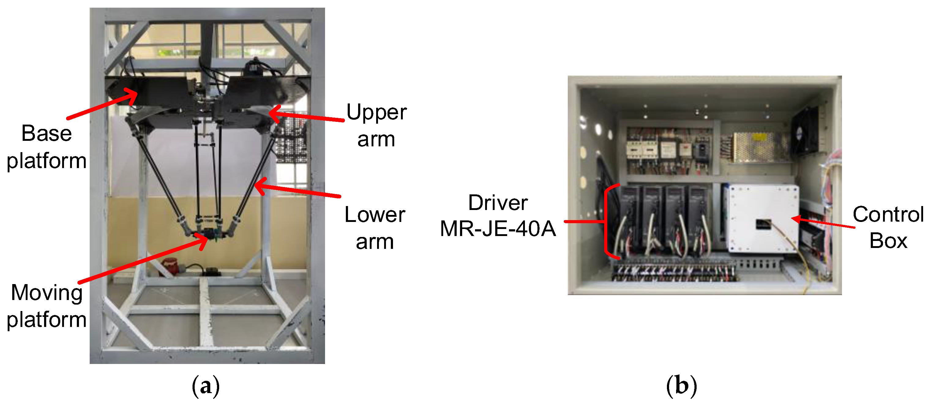
An experiment testbench is built, as shown in Figure 5, including a 4-DOF parallel manipulator and a control cabinet. Firstly, a 4-DOF parallel manipulator is formed using a base platform made of steel, four upper arms and four lower arms made of aluminum and carbon, and a moving platform made of plastic. Four AC servo motors Mitsubishi 400 W and four gears rate 1:25 actives for four arms make up the move end-effector, following the preset trajectory, which is attached on a moving platform. Secondly, a control cabinet to control a 4-DOF parallel robot consists of a four-driver MR-JE-40A to the amplifier control signal for four AC Servo, a control box that provides voltage control signals for four-drive MR-JE-40A, according to the torque control mode and the electric devices, such as a circuit break, contractor, noise filter module, and DC supply voltage module. Finally, the operating process of the system is described in Figure 6.
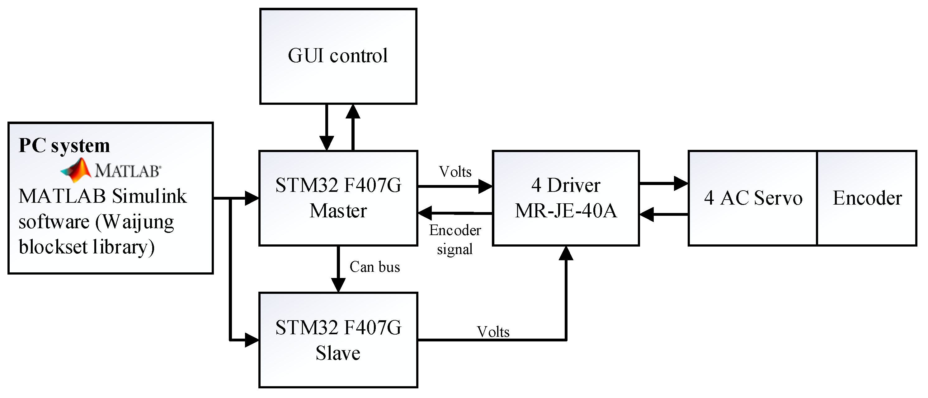
Based on Figure 6, the controllers are built on the MATLAB Simulink 2019a using the Waijung block set library. After that, these programs are embedded into the STM32 F407G board. There are two STM32 F407G boards used here, and they communicate via the Can bus protocol. Each STM32 F407G board provides a signal control for two-drive MR-JE-40A and makes the AC Servo motos run. For the STM32 F407G Master board, it not only provides a control signal for the drivers but also reads the encoder signals from motors through the corresponding drives at each joint. Furthermore, the STM32 F407G Master board also receives control commands from Gui control and shows the responses of the system intuitively.

4.2. Experiment Index

This section presents the experimental index of three controllers on a 4-DOF parallel robot: PD, SPD, and SPD-TDE. The controllers are programmed on MATLAB Simulink 2019a and integrated into the Waijung block set library to support the embedded program for the STM32 board to provide analog control signals to the motor driver. Moreover, a circle trajectory, as calculated using expression (38), is set with the execution time of 40 s. The operating frequency is 0.2 π . The radius is 100 mm. The sampling time of the system is 0.005 s, and the Solver type is auto.
P x = 100 cos 0.2 π t   P y = 100 sin 0.2 π t P z = 500
Next, the control coefficients are presented in Table 2.
Remark 3.
The parameters K P 1 , K D 1 of the PD control are selected via the trial-and-error method. Consequently, when incorporating the synchronous method into the PD control, β 2 is also designed and selected according to trial and error, starting from 0, with a step size of 0.1. For the proposed control method SPD-TDE, the robot operates effectively in reality. The control coefficients are selected according to the given conditions. The parameter in the diagonal matrix M ¯ must be selected according to the stability condition presented in Equation (25). Then, the coefficient K P * , K D * of the SPD-TDE control is selected with the initial reference value based on the following relationship K P 1 , 2 = M ¯ K P * , K D 1 , 2 = M ¯ K D * . Finally, the delay time is the selected sampling time of the system, and the value of the synchronous coefficient matrix β * is also selected similarly to the PD control and SPD control.
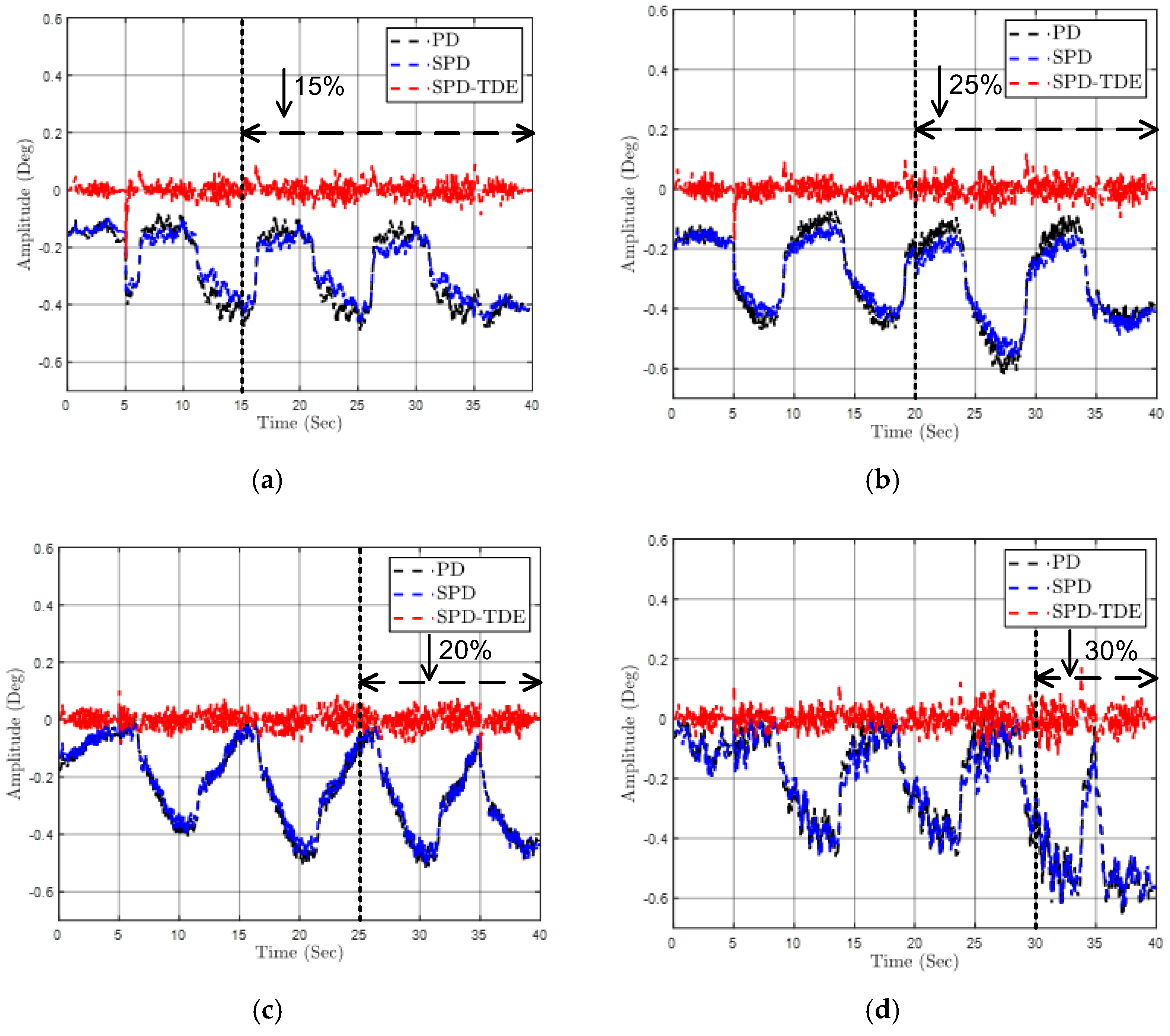
In addition, to better demonstrate the effectiveness of the proposed controller, the modeling error and actuator faults are put into the experimental process. The modeling error exists in the N q , q ˙ , q ¨ term of the Formula (10). Actuator faults or the loss of efficiency faults of the motors will occur during the operation, and this is expressed via the coefficient α in Formula (9). In summary, there are three case studies conducted in this study. In case study 1, the robot operates normally, and there no losses of efficiency faults α = d i a g 1 1 1 1 . In case study 2, the robot operates with 2 kg load with α = d i a g 1 1 1 1 . In case study 3, the robot operates under the affected with a loss of efficiency of the motors during the operation according to the following scenarios: at the 10th second, the efficiency of motor 1 is reduced by 15% α = d i a g 0.85 1 1 1 ; at the 15th second, the efficiency of motor 3 is reduced by 20% α = d i a g 0.85 1 0.8 1 ; at the 20th second the efficiency of the motor 2 reduce by 25% α = d i a g 0.85 0.75 0.8 1 ; and at the 30th second, the efficiency of the motor 4 is reduced by 30% α = d i a g 0.85 0.75 0.8 0.7 .
Finally, a well-known method to evaluate the standard deviation of the errors is called the root-mean-square error (RMSE), and the mathematical expressions are presented as Formula (39). In this study, the RMSE is used to evaluate the errors in case studies 1, 2, and 3 and to prove most clearly the effectiveness of the proposed method.
R M S E = 1 n i = 1 n s i o i 2
where n is samples of modeling errors, s i is the desired value, o i is the response value, and i is a variable.

4.3. Experiment Results

Case Study 1:
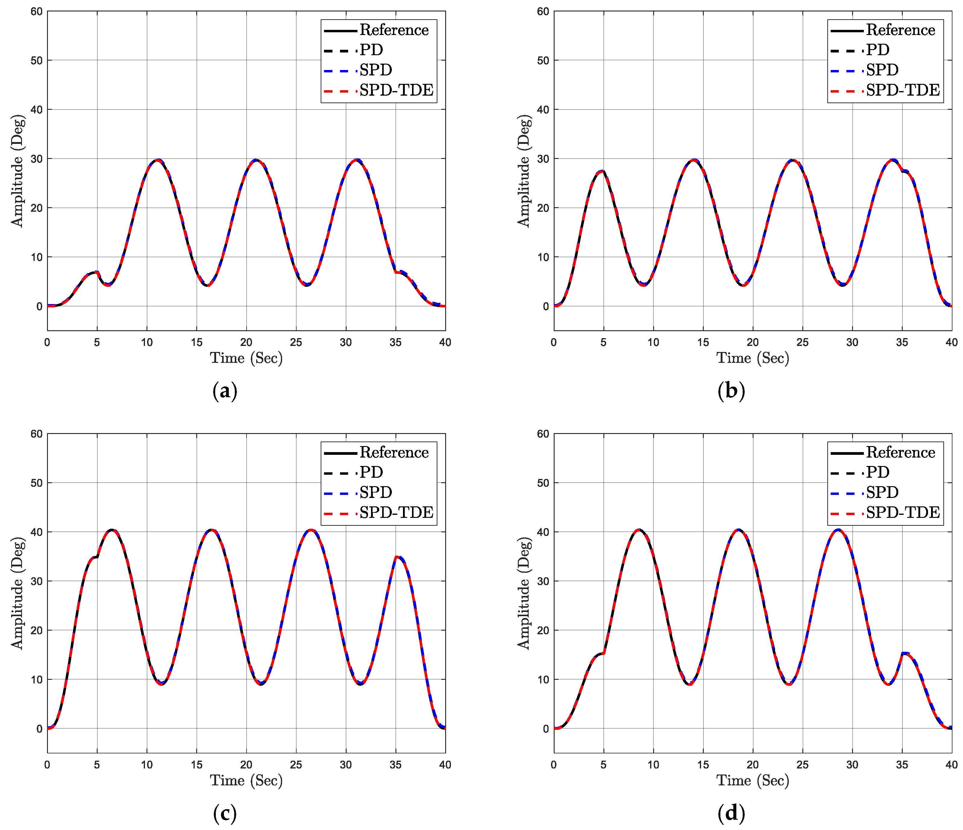
During the experiment of the robot, data, such as the response of the joint angle, tracking error, synchronous error, and the control signal of three controllers, PD, SPD, and SPD-TDE, were collected to visually describe the state of the robot corresponding to each controller. Firstly, the joint angle response relative to the desired signal is presented in Figure 7.
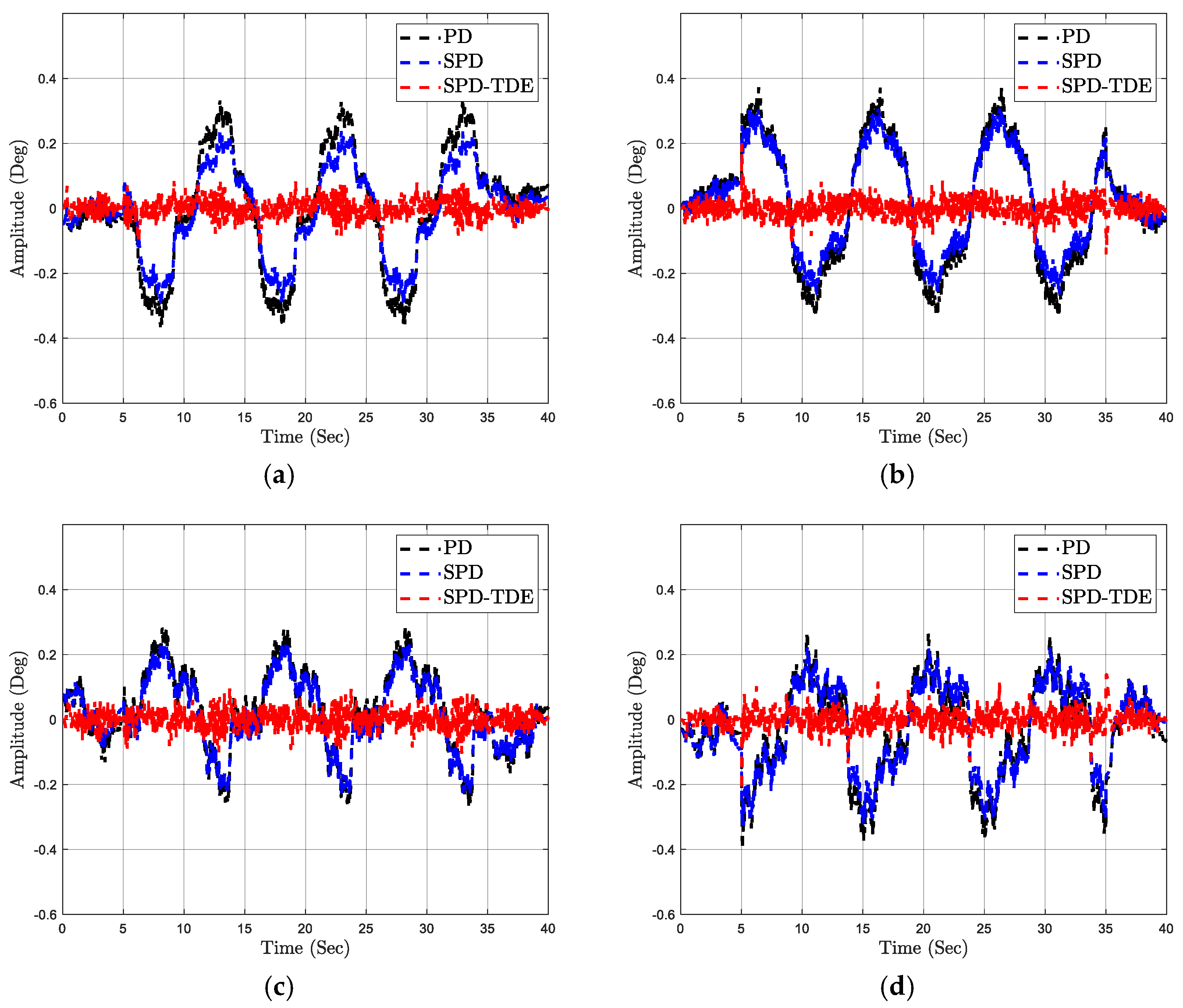
The desired and response signals at the four joint angles relative to the reference signal corresponding to each controller are described in Figure 7. The solid black line is the reference signal, and the dashed black line is the response signal of the joint angles when using the PD control. Likewise, the dashed blue line is for the SPD control, and the dashed red line is for the SPD-TDE control. Based on Figure 7, we can see that the response of the joint angles of the three controllers compared to the desired signal is very good. Therefore, to see more clearly the effectiveness of the proposed method or the difference between the response signal and the desired signal, the tracking error at each joint angle of the three controllers is shown in the following figure.
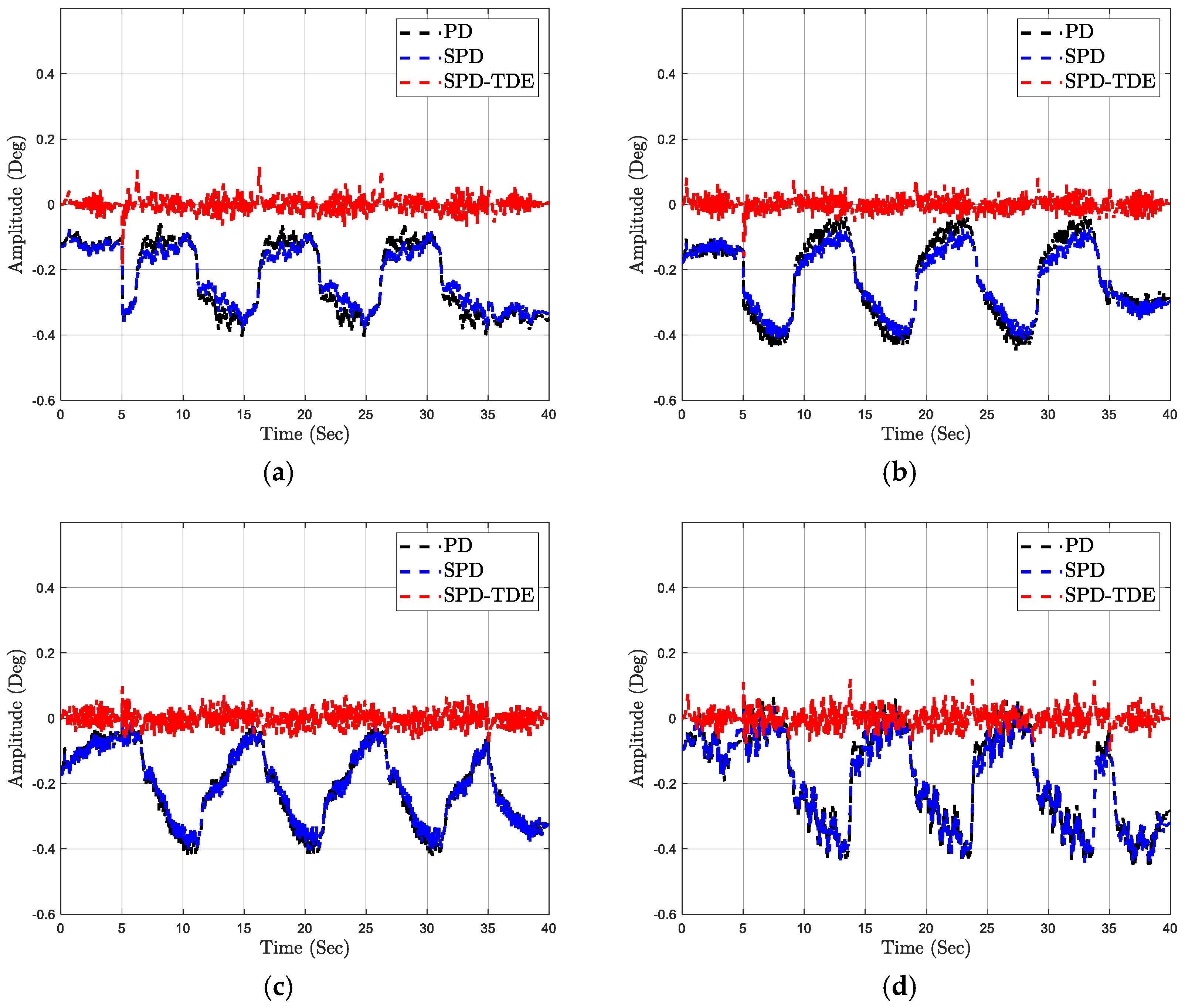
Figure 8 shows the tracking error at each active joint of the robot according to time. The dashed black line shows the tracking error of the joint angles when using the PD control, the dashed blue line shows the tracking error of the SPD control, and the dashed red line shows the tracking error of the SPD-TDE control. Based on Figure 8, we can see that the tracking error of the SPD control and SPD-TDE control is better than the asynchronous PD control. In there, the SPD-TDE control is designed based on TDE; thanks to this combination, the nonlinear and uncertain components of the system are eliminated. Therefore, the tracking error of the SPD-TDE control gives the best tracking error compared to the other controllers. Next, to demonstrate the necessity of the synchronous method for robots with closed-loop structures that have many constraints on the fixed base and the movable base, the synchronous error is presented, as shown in the figure below.
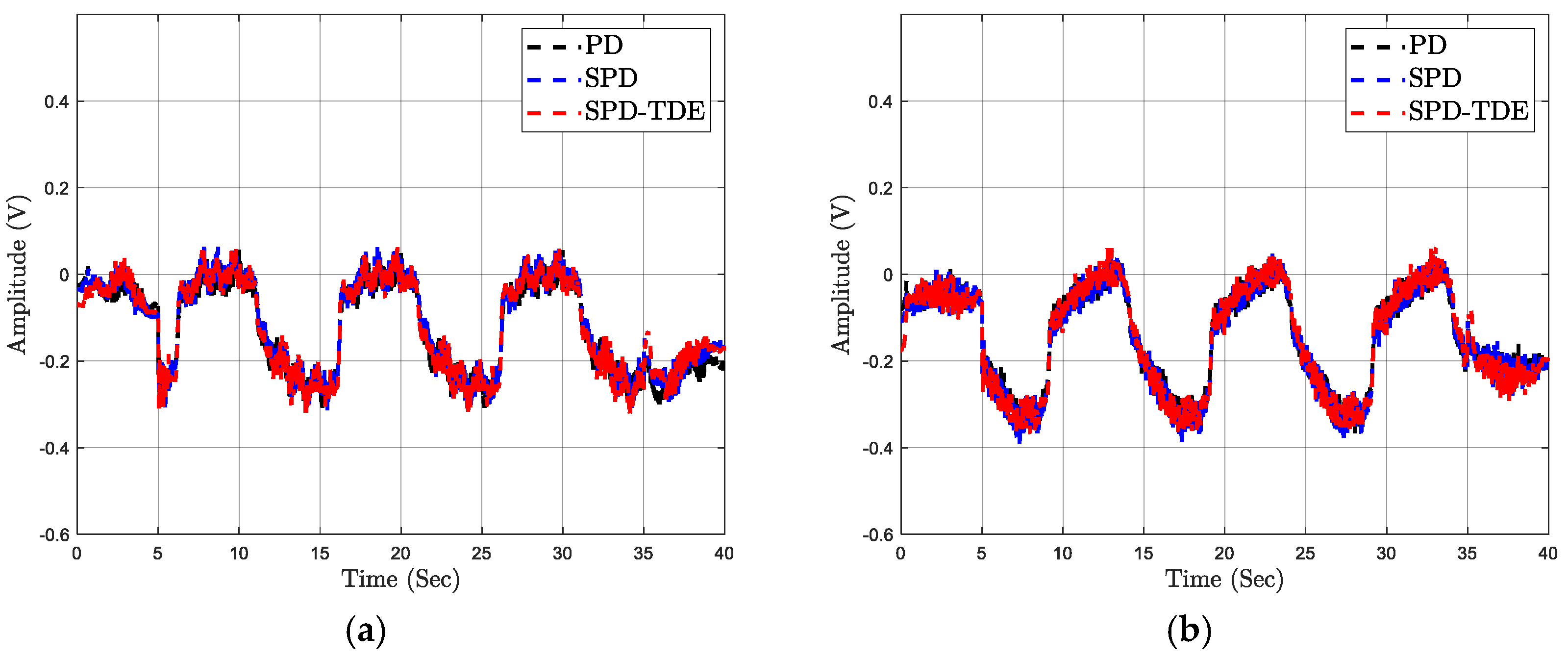
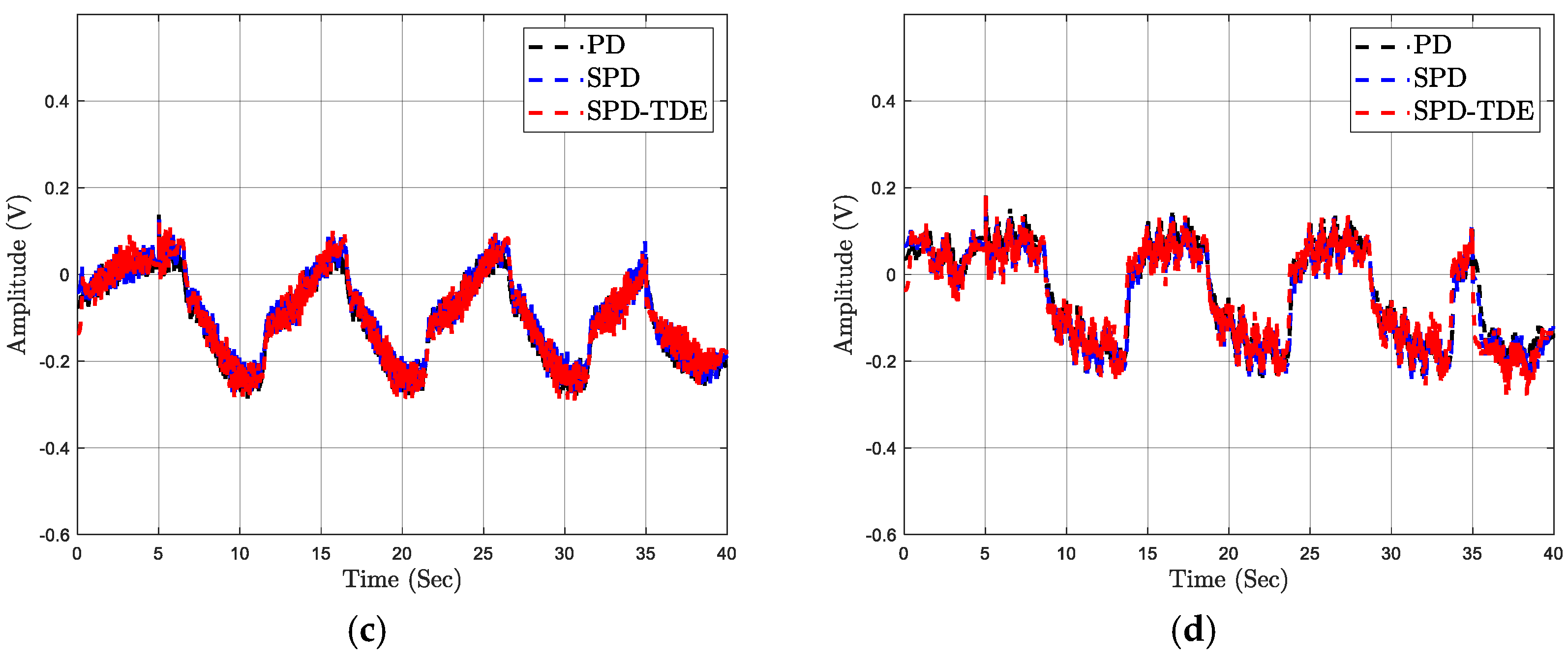
Figure 9 displays the synchronous error between the joints as well as the difference in the position error between two adjacent joints. The dashed black line is the synchronous error of the PD control. The dashed blue line is the synchronous error of the SPD controller. The dashed red line is the synchronous error of the SPD-TDE control. Based on the data in Figure 9, we can see that the synchronous error of the asynchronous PD control is larger than the two controls combined with the synchronous algorithm: SPD and SPD-TDE. With the synchronous interest, the tracking and synchronous errors are proportional to each other. Specifically, asynchronous controllers will have large synchronous errors leading to large tracking errors and contrast. Besides that, the synchronous error of the proposed control still gives the best results. Thereby, the robustness of the TDE method when combined with the synchronous method in this study is confirmed. Next, the control signal at each joint of the robot is presented in Figure 10 below.
Generally, the evaluation of the effectiveness of the proposed method by observing the graph is only the objective of the observer. Therefore, to increase persuasion, the RMSE method calculates the root-mean-square error of the tracking error and the synchronous error in this case. The calculation results are presented in Table 3 and Table 4.
Based on Table 3 and Table 4, we can conclude that the proposed method SPD-TDE has the best error quality compared to the remaining controllers. Next, to see the effectiveness of the synchronous and TDE method applied to a 4-DOF parallel robot. In case study 2, we carried out the robot carrying a load of 2 kg during the operation process.
Case Study 2:
In this case, the robot is loaded with a mass of 2 kg. Then, the tracking error at each joint of the robot is presented in Figure 11.
Based on Figure 11, when the robot is loaded, the tracking performance of the controllers decreases. However, thanks to the compensation of uncertainty components in the system of the TDE method, the tracking quality of the SPD-TDE method is still better than the other controllers. Moreover, carrying the load also makes the robot deviation larger between the joints of the robot, and the synchronous method also overcomes this problem. Therefore, the tracking quality of the SPD is better than the asynchronous PD control. Next, the synchronous error of the robot is shown in Figure 12.
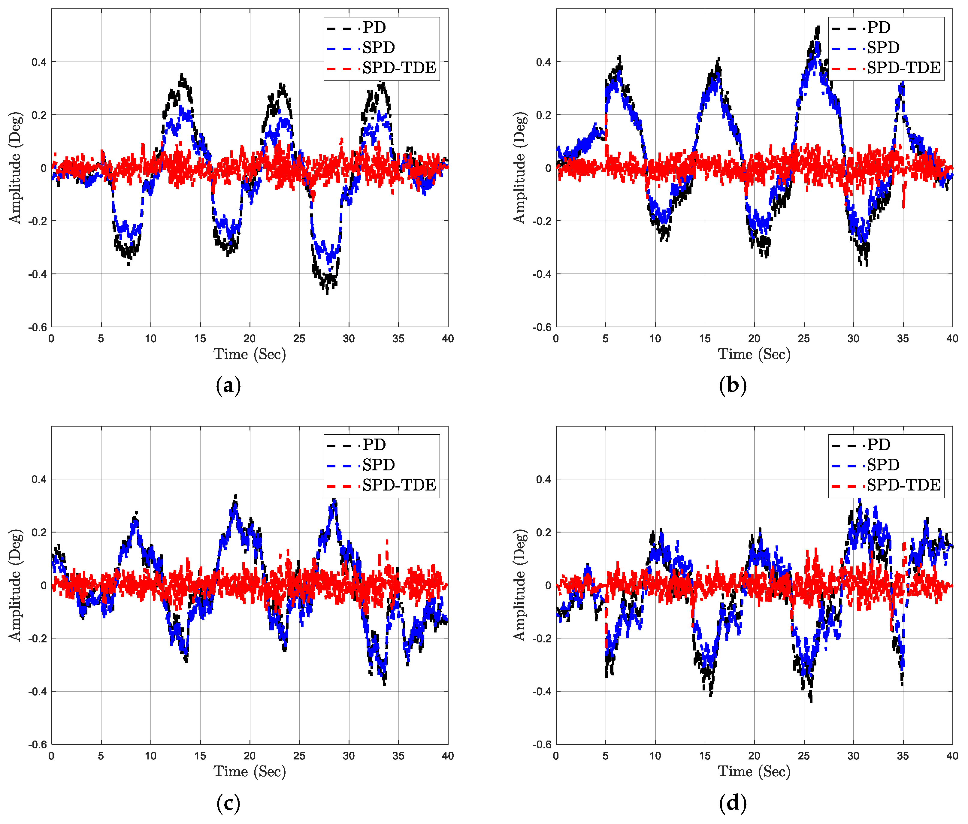
Figure 12 shows the synchronous error between two adjacent joints of the robot. Thanks to the characteristics of the closed-loop structure, the load will be equally shared for each kinematic chain of the robot. However, the reduction in the synchronous performance of the robot still occurs. But the application of the synchronous algorithm has significantly improved the tracking quality of the SPD and SPD-TDE controllers. In particular, the SPD-TDE controller gives much better synchronous error results than other controllers thanks to the compensation of dynamic components in the system.
In addition, the root-mean-square error of the tracking error and synchronous error are also calculated and shown in Table 5 and Table 6.
From Table 5 and Table 6, we can see that the error quality of the synchronous control is better than the asynchronous control. Moreover, the ability to estimate and eliminate the uncertainty term in the system. So, the control method SPD-TDE obtains the smallest error.
Next, to see the robustness of combining the SPD control method with the TDE method, in case study 3, actuator faults in the system are established on the real model, as mentioned in the experiment index.
Case study 3:
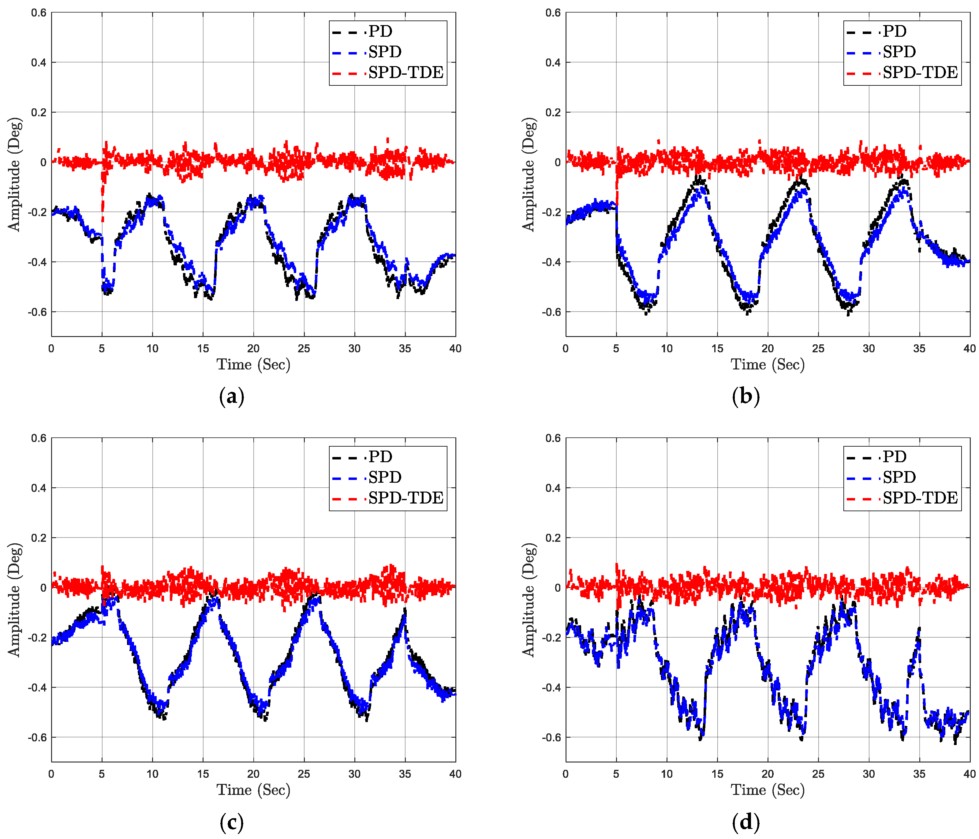
In this case, the loss of efficiency of the motors during the operation will be introduced into the system to demonstrate the effectiveness of the proposed method. Firstly, the tracking error at each joint is shown in Figure 13.
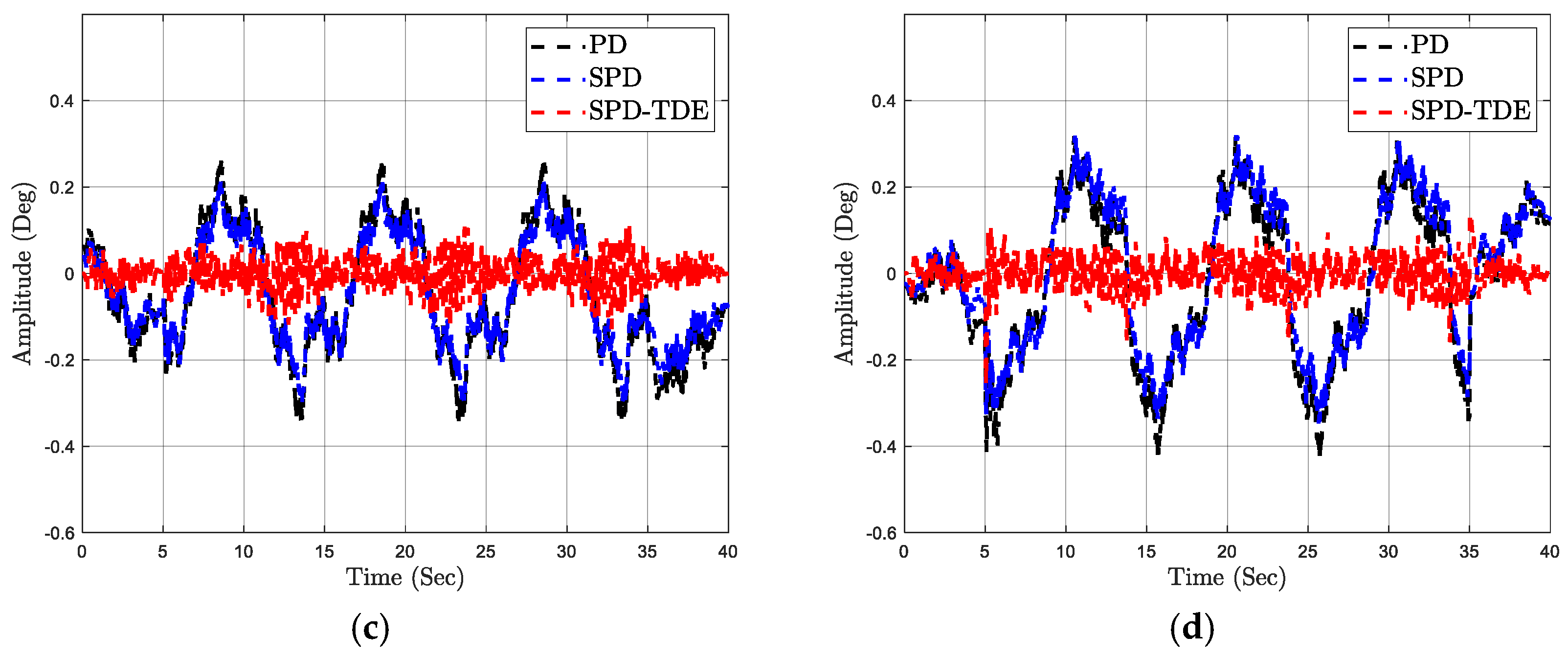
Figure 13 shows the tracking error at each joint in the case of the influence of modeling error and actuator faults. Based on the figure, we can see that although there are adverse effects on the system, the sustainability of the proposed method is still strongly shown. Specifically, the tracking error of the SPD-TDE control is much better than the tracking error of the PD control and the SPD control. Next, the synchronous error, in this case, is shown in Figure 14.
Figure 14 shows the synchronous error between the joints of the robot. When modeling errors and actuator faults, the errors are impacted at different times, and the deviation between joints occurs, leading to asynchrony between joints. At that time, the robustness of the synchronous method is promoted. As a result, the synchronous error of the SPD control and the SPD-TDE control is better than the asynchronous PD control, and the error of the SPD-TDE control is the smallest.
In this case, the root-mean-square error is calculated and expressed in Table 7 and Table 8.
From Table 7 and Table 8, we can realize that the error quality of the SPD-TDE control is much smaller than the other controllers, and the SPD control has an error quality better than the PD control. From that, the effectiveness of the proposed method is revealed when applied to a 4-DOF parallel robot. The operating performance of the system, as well as the capability trajectory tracking of the end-effector, has improved significantly.

5. Conclusions

This paper proposed the SPD-TDE control for a 4-DOF parallel manipulator under the existence of nonlinear and uncertain components in the system, including modeling error and actuator faults. The proposed control is built based on the combination of SPD control with the TDE method. The 4-DOF parallel robot system has a closed-loop structure, and the binding occurs between the fixed base and the movable base via the identical kinematic sequences. At that time, the synchronous method solved the asynchronous problem between the joints of the robot by designing a synchronous algorithm based on the cross-coupling error. When the cross-coupling error converges to zero or when both the tracking and synchronous errors converge to zero simultaneously, the synchronous aim has been accomplished. In addition, the TDE method provided a simple control structure and eliminated the nonlinear and uncertain components in the system using time-delayed information. As a result, the operating performance of the robot and trajectory tracking quality are significantly improved. The experimental process is divided into three different case studies, and the results of the proposed control are compared with the PD control and SPD control to demonstrate the sustainability and effectiveness of the proposed method.

Author Contributions

Conceptualization, D.T.T., T.N.N. and X.T.N.; methodology, D.T.T., T.N.N. and X.T.N.; software, X.T.N. and D.M.N.; validation, T.N.N., X.T.N. and D.M.N.; formal analysis, T.N.N., X.T.N. and D.M.N.; investigation, D.T.T.; resources, D.T.T.; data curation T.N.N., X.T.N. and D.M.N.; writing—original draft preparation, T.N.N., X.T.N. and D.M.N.; writing—review and editing, D.T.T.; visualization, X.T.N. and D.M.N.; supervision, D.T.T.; project administration, D.T.T.; funding acquisition, D.T.T. All authors have read and agreed to the published version of the manuscript.

Funding

This work belongs to the project grant No: B2022-SPK-03. funded by Ministry of Education and Training and hosted by Ho Chi Minh City University of Technology and Education, Vietnam.

Data Availability Statement

Not applicable.

Conflicts of Interest

The authors declare no conflict of interest.

Appendix A

For the first arm, the formula of E 1 , F 1 , and G 1 is presented as follows:
E 1 = 2 L 1 Z F 1 = 2 L 1 r 2 L 1 X cos α 1 L 1 d cos α 1 2 L 1 d 1 cos α 1 2 L 1 Y sin α 1 2 L 1 h 1 sin α 1 + 2 L 1 h cos α 1 sin θ 2 L 1 h sin α 1 cos θ G 1 = E 1 sin q 1 F 1 cos q 1
For the second arm, the formula of E 2 , F 2 , and G 2 is presented as follows:
E 2 = 2 L 1 Z F 2 = 2 L 1 r 2 L 1 X cos α 2 + L 1 d cos α 2 + 2 L 1 d 2 cos α 2 2 L 1 Y sin α 2 2 L 1 h 2 sin α 2 + 2 L 1 h cos α 2 sin θ 2 L 1 h sin α 2 cos θ G 2 = E 2 sin q 2 F 2 cos q 2
For the third arm, the formula of E 3 , F 3 , and G 3 is presented as follows:
E 3 = 2 L 3 Z F 3 = 2 L 1 r 2 L 1 X cos α 3 + L 1 d cos α 3 + 2 L 1 d 3 cos α 3 2 L 1 Y sin α 3 + 2 L 1 h 3 sin α 3 G 3 = E 3 sin q 3 F 3 cos q 3
For the fourth arm, the formula of E 4 , F 4 and G 4 is presented as follows:
E 4 = 2 L 4 Z F 4 = 2 L 1 r 2 L 1 X cos α 4 L 1 d cos α 4 2 L 1 d 4 cos α 3 2 L 1 Y sin α 4 + 2 L 1 h 4 sin α 4 G 4 = E 4 sin q 4 F 3 cos q 4

References

  1. Xu, L.; Li, Y. Investigation of joint clearance effects on the dynamic performance of a planar 2-DOF pick-and-place parallel manipulator. Robot. Comput. Integr. Manuf. 2014, 30, 62–73. [Google Scholar]
  2. Wang, D.; Wu, J.; Wang, L.; Liu, Y. A Postprocessing Strategy of a 3-DOF Parallel Tool Head Based on Velocity Control and Coarse Interpolation. IEEE Trans. Ind. Electron. 2018, 65, 6333–6342. [Google Scholar]
  3. Bourbonnais, F.; Bigras, P.; Bonev, I.A. Minimum-Time Trajectory Planning and Control of a Pick-and-Place Five-Bar Parallel Robot. IEEE/ASME Trans. Mechatron. 2015, 20, 740–749. [Google Scholar] [CrossRef]
  4. Gonzalez-de-Santos, P.; Fernández, R.; Sepúlveda, D.; Navas, E.; Emmi, L.; Armada, M. Field Robots for Intelligent Farms—Inhering Features from Industry. Agronomy 2020, 10, 1638. [Google Scholar] [CrossRef]
  5. Musa, M.; Sengupta, S.; Chen, Y. Design of a 6-DoF Parallel Robotic Platform for MRI Applications. J. Med. Robot. Res. 2022, 7, 2241005. [Google Scholar] [CrossRef]
  6. Dasgupta, B.; Mruthyunjaya, T.S. The Stewart platform manipulator: A review. Mech. Mach. Theory 2000, 35, 15–40. [Google Scholar] [CrossRef]
  7. Pandilov, Z.; Dukovski, V. Comparison of the characteristics between serial and parallel robots. Acta Tech. Corviniensis-Bull. Eng. 2014, 7, 143–160. [Google Scholar]
  8. Ghorbel, F.H.; Chetelat, O.; Gunawardana, R.; Longchamp, R. Modeling and set point control of closed-chain mechanisms: Theory and experiment. IEEE Trans. Control Syst. Technol. 2000, 8, 801–815. [Google Scholar] [CrossRef] [Green Version]
  9. Villarreal-Cervantes, M.G.; Alvarez-Gallegos, J. Off-line PID control tuning for a planar parallel robot using DE variants. Expert Syst. Appl. 2016, 64, 444–454. [Google Scholar] [CrossRef]
  10. Azmoun, M.; Rouhollahi, A.; Masouleh, M.T.; Kalhor, A. Kinematics and Control of a 4-DOF Delta Parallel Manipulator. In Proceedings of the 2018 6th RSI International Conference on Robotics and Mechatronics (IcRoM), Tehran, Iran, 23–25 October 2018; pp. 494–500. [Google Scholar]
  11. Hadoune, O.; Benouaret, M. Fuzzy-PID tracking control of a ball and plate system using a 6 Degrees-of-Freedom parallel robot. In Proceedings of the 2022 19th International Multi-Conference on Systems, Signals & Devices (SSD), Setif, Algeria, 6–10 May 2022; pp. 1906–1912. [Google Scholar]
  12. Jin, L.; Li, S.; Yu, J.; He, J. Robot manipulator control using neural networks: A survey. Neurocomputing 2018, 285, 23–34. [Google Scholar] [CrossRef]
  13. Liu, S.; Peng, G.; Gao, H. Dynamic modeling and terminal sliding mode control of a 3-DOF redundantly actuated parallel platform. Mechatronics 2019, 60, 26–33. [Google Scholar] [CrossRef]
  14. Soriano, L.A.; Rubio, J.D.; Orozco, E.; Cordova, D.A.; Ochoa, G.; Balcazar, R.; Cruz, D.R.; Meda-Campaña, J.A.; Zacarias, A.; Gutierrez, G.J. Optimization of Sliding Mode Control to Save Energy in a SCARA Robot. Mathematics 2021, 9, 3160. [Google Scholar] [CrossRef]
  15. Mazare, M.; Taghizadeh, M.; Ghaf-Ghanbari, P. Fault-tolerant control based on adaptive super-twisting nonsingular integral-type terminal sliding mode for a delta parallel robot. J. Braz. Soc. Mech. Sci. Eng. 2020, 42, 443. [Google Scholar] [CrossRef]
  16. Godbole, H.A.; Caverly, R.J.; Forbes, J.R. Dynamic Modeling and Adaptive Control of a Single Degree-of-Freedom Flexible Cable-Driven Parallel Robot. J. Dyn. Syst. Meas. Control 2019, 141, 101002. [Google Scholar] [CrossRef]
  17. Yao, S.; Gao, G.; Gao, Z.; Li, S. Active disturbance rejection synchronization control for parallel electro-coating conveyor. ISA Trans. 2020, 101, 327–334. [Google Scholar] [CrossRef] [PubMed]
  18. Koren, Y. Cross-Coupled Biaxial Computer Control for Manufacturing Systems. J. Dyn. Syst. Meas. Control 1980, 102, 265–272. [Google Scholar] [CrossRef]
  19. Sun, D.; Tong, M.C. A Synchronization Approach for the Minimization of Contouring Errors of CNC Machine Tools. IEEE Trans. Autom. Sci. Eng. 2009, 6, 720–729. [Google Scholar]
  20. Zhong, G.; Shao, Z.; Deng, H.; Ren, J. Precise Position Synchronous Control for Multi-Axis Servo Systems. IEEE Trans. Ind. Electron. 2017, 64, 3707–3717. [Google Scholar] [CrossRef]
  21. Sun, D. Position synchronization of multiple motion axes with adaptive coupling control. Automatica 2003, 39, 997–1005. [Google Scholar] [CrossRef]
  22. Xu, J.; Lu, H.; Liu, X. Synchronization control strategy in multi-layer and multi-axis systems based on the combine cross coupling error. Adv. Mech. Eng. 2017, 9, 1687814017711392. [Google Scholar] [CrossRef]
  23. Sun, D.; Lu, R.; Mills, J.K.; Wang, C. Synchronous Tracking Control of Parallel Manipulators Using Cross-coupling Approach. Int. J. Robot. Res. 2006, 25, 1137–1147. [Google Scholar] [CrossRef]
  24. Shang, W.; Cong, S.; Jiang, S. Synchronization control of a parallel manipulator with redundant actuation in the task space. Int. J. Robot. Autom. 2011, 26, 432. [Google Scholar] [CrossRef]
  25. Wos, P.; Dindorf, R. Synchronized Trajectory Tracking Control of 3-DoF Hydraulic Translational Parallel Manipulator. In Mechatronics—Ideas for Industrial Application; Springer International Publishing: Cham, Switzerland, 2015; pp. 269–277. [Google Scholar]
  26. Shi, K.; Liu, C.; Sun, Z.; Yue, X. Coupled orbit-attitude dynamics and trajectory tracking control for spacecraft electromagnetic docking. Appl. Math. Model. 2022, 101, 553–572. [Google Scholar] [CrossRef]
  27. Tran, D.T.; Nha, N.T.; Phung, M.V.; Long, N.P.; Tam, N.M.; Ahn, K.K. Synchronous PID controller for a 4-DOF parallel manipulator in practice. In Proceedings of the 2022 25th International Conference on Mechatronics Technology (ICMT), Kaohsiung, Taiwan, 18–21 November 2022; pp. 1–4. [Google Scholar]
  28. Zhou, J.; Liu, E.; Tian, X.; Li, Z. Adaptive Fuzzy Backstepping Control Based on Dynamic Surface Control for Uncertain Robotic Manipulator. IEEE Access 2022, 10, 23333–23341. [Google Scholar] [CrossRef]
  29. Liu, C.; Yue, X.; Zhang, J.; Shi, K. Active Disturbance Rejection Control for Delayed Electromagnetic Docking of Spacecraft in Elliptical Orbits. IEEE Trans. Aerosp. Electron. Syst. 2022, 58, 2257–2268. [Google Scholar] [CrossRef]
  30. Cho, S.-j.; Jin, M.; Kuc, T.-Y.; Lee, J.S. Control and synchronization of chaos systems using time-delay estimation and supervising switching control. Nonlinear Dyn. 2014, 75, 549–560. [Google Scholar] [CrossRef]
  31. Hyo-Jeong, B.; Maolin, J.; Jinho, S.; Jun Young, L.; Pyung-Hun, C.; Doo-sung, A. Control of Robot Manipulators Using Time-Delay Estimation and Fuzzy Logic Systems (in Korean). J. Electr. Eng. Technol. 2017, 12, 1271–1279. [Google Scholar]
  32. Wang, Y.; Peng, J.; Zhu, K.; Chen, B.; Wu, H. Adaptive PID-fractional-order nonsingular terminal sliding mode control for cable-driven manipulators using time-delay estimation. Int. J. Syst. Sci. 2020, 51, 3118–3133. [Google Scholar] [CrossRef]
  33. Duong, T.T.; Nguyen, C.C.; Tran, T.D. Synchronization Sliding Mode Control of Closed-Kinematic Chain Robot Manipulators with Time-Delay Estimation. Appl. Sci. 2022, 12, 5527. [Google Scholar] [CrossRef]
  34. Duong, T.T.C.; Thien, T.D.; Tri, N.T.; Nghi, D.V. Synchronization Sliding Mode Control with Time-Delay Estimation for a 2-DOF Closed-Kinematic Chain Robot Manipulator. In Proceedings of the 2021 International Conference on System Science and Engineering (ICSSE), Ho Chi Minh City, Vietnam, 26–28 August 2021; pp. 38–43. [Google Scholar]
  35. Corbel, D.; Nabat, V.; Maurine, P. Geometrical calibration of the high speed robot Par4 using a laser tracker. In Proceedings of the MMAR’06: 12th International Conference on Methods and Models in Automation and Robotics, Miedzyzdroje, Poland, 28–31 August 2006; pp. 687–692. [Google Scholar]
  36. M’hiri, S.A.; Ben Romdhane, N.M.; Damak, T. New Forward Kinematic Model of Parallel Robot Par4. J. Intell. Robot. Syst. 2019, 96, 283–295. [Google Scholar] [CrossRef]
  37. Hsia, T.C.; Gao, L.S. Robot manipulator control using decentralized linear time-invariant time-delayed joint controllers. In Proceedings of the IEEE International Conference on Robotics and Automation, Cincinnati, OH, USA, 13–18 May 1990; Volume 3, pp. 2070–2075. [Google Scholar]
Figure 1. The 3D model of a 4-DOF parallel robot.
Machines 11 00831 g001
Figure 2. The geometry structure of a 4-DOF parallel manipulator: (a) Top view of a base platform; (b) Side view of a chain kinematic ith; and (c) Top view of a moving platform.
Machines 11 00831 g002
Figure 3. The structure of the synchronous PD control.
Machines 11 00831 g003
Figure 4. The structure of the proposed control.
Machines 11 00831 g004
Figure 5. An experimental testbench: (a) 4-DOF parallel manipulator; (b) Control cabinet.
Machines 11 00831 g005
Figure 6. Description of the operating structure of the system.
Machines 11 00831 g006
Figure 7. Desired and response signals at the joints: (a) Joint 1; (b) Joint 2; (c) Joint 3; and (d) Joint 4.
Machines 11 00831 g007
Figure 8. Tracking error at each joint: (a) Joint 1; (b) Joint 2; (c) Joint 3; and (d) Joint 4.
Machines 11 00831 g008
Figure 9. Synchronous error among the joints: (a) Joints 1 and 2; (b) Joints 2 and 3; (c) Joints 3 and 4; and (d) Joints 4 and 1.
Machines 11 00831 g009
Figure 10. Signal control input at each joint: (a) Joint 1; (b) Joint 2; (c) Joint 3; and (d) Joint 4.
Machines 11 00831 g010aMachines 11 00831 g010b
Figure 11. Tracking error at each joint: (a) Joint 1; (b) Joint 2; (c) Joint 3; and (d) Joint 4.
Machines 11 00831 g011
Figure 12. Synchronous error among the joints: (a) Joints 1 and 2; (b) Joints 2 and 3; (c) Joints 3 and 4; and (d) Joints 4 and 1.
Machines 11 00831 g012aMachines 11 00831 g012b
Figure 13. Tracking error at each joint: (a) Joint 1; (b) Joint 2; (c) Joint 3; and (d) Joint 4.
Machines 11 00831 g013
Figure 14. Synchronous errors among the joints: (a) Joints 1 and 2; (b) Joints 2 and 3; (c) Joints 3 and 4; and (d) Joints 4 and 1.
Machines 11 00831 g014
Table 1. The physic parameters of the 4-DOF parallel robot experiment.
ParametersValueDescription
L 1 181 mmLength of an active limb
L 2 498 mmLength of a passive limb
r 136.5 mmRadius of fixed base
d 80 mmLength of the moving platform
h 80 mmLength of the moving platform’s parallelogram bars
h i , d i i = 1 , 2 , 3 , 4 20.7 mmDistances between C i and D i , respectively, along P Y axis and along P X axis
Table 2. The parameters of the controllers.
ControllersParameters
PD K P 1 = diag 55 55 53.5 40 , K D 1 = diag 0.5 0.5 0.45 0.25
SPD K P 2 = diag 55 55 53.5 40 , K D 2 = diag 0.5 0.5 0.45 0.25 , β 2 = diag 0.15 0.15 0.15 0.15
SPD-TDE K P * = d i a g 4200   4200   4150   4100 , K D * = d i a g 400   40 0   395   39 0 , β * = d i a g 0.15   0.15   0.15   0.15 , M ¯ = d i a g 0.0006   0.0006   0.0006   0.0006 , L = 0.005
Table 3. Root-mean-square error of the tracking error at each joint.
ControllersJoint 1Joint 2Joint 3Joint 4
PD0.24930.25900.23930.2357
SPD0.23970.25370.23330.2355
SPD-TDE0.02160.02070.02180.0270
Table 4. Root-mean-square error of the synchronous error among two adjacent joints.
ControllersJoints 1 and 2Joints 2 and 3Joints 3 and 4Joints 4 and 1
PD0.17810.18340.12330.1437
SPD0.13280.15300.11000.1342
SPD-TDE0.02640.02750.02710.0297
Table 5. Root-mean-square error of the tracking error at each joint.
ControllersJoint 1Joint 2Joint 3Joint 4
PD0.35900.35250.30620.3618
SPD0.34000.34520.30320.3602
SPD-TDE0.02710.02530.02600.0285
Table 6. Root-mean-square error of the synchronous error among two adjacent joints.
ControllersJoints 1 and 2Joints 2 and 3Joints 3 and 4Joints 4 and 1
PD0.23080.24080.15120.1767
SPD0.18370.19750.13100.1704
SPD-TDE0.03370.03050.03240.0364
Table 7. Root-mean-square error of the tracking error at each joint.
ControllersJoint 1Joint 2Joint 3Joint 4
PD0.35900.35250.30620.3618
SPD0.34000.34520.30320.3602
SPD-TDE0.02710.02530.02600.0285
Table 8. Root-mean-square error of the synchronous error among two adjacent joints.
ControllersJoints 1 and 2Joints 2 and 3Joints 3 and 4Joints 4 and 1
PD0.23080.24080.15120.1767
SPD0.18370.19750.13100.1704
SPD-TDE0.03370.03050.03240.0364
Disclaimer/Publisher’s Note: The statements, opinions and data contained in all publications are solely those of the individual author(s) and contributor(s) and not of MDPI and/or the editor(s). MDPI and/or the editor(s) disclaim responsibility for any injury to people or property resulting from any ideas, methods, instructions or products referred to in the content.