Article

Fault Diagnosis of Train Wheelset Bearing Roadside Acoustics Considering Sparse Operation with GA-RBF

1
College of Mechanical and Electrical Engineering, Lanzhou Jiaotong University, Lanzhou 730070, China
2
College of Automation and Electrical Engineering, Lanzhou Jiaotong University, Lanzhou 730070, China
*
Author to whom correspondence should be addressed.
Machines 2023, 11(7), 765; https://doi.org/10.3390/machines11070765
Submission received: 11 June 2023 / Revised: 19 July 2023 / Accepted: 19 July 2023 / Published: 22 July 2023
(This article belongs to the Section Machines Testing and Maintenance)

Abstract

:
Trackside acoustic signals are useful for non-contact measurements as well as early warnings in the diagnosis of train wheelset bearing faults. However, there are two important problems when using roadside acoustic signals to diagnose wheel-to-wheel bearing faults; one is the presence of strong interference from strong noise and high harmonics in the signal, and the other is the low efficiency of bearing fault identification caused by it. Therefore, from the viewpoint of solving the two problems, a sparse operation method is proposed for denoising and detuning the modulation of the roadside acoustic signal, and a machine learning classifier with a Genetic Algorithm (GA)-optimized Radial Basis Neural Network (RBFNN) is proposed to improve the rate at which the features of roadside acoustic signal faults are recognized. Firstly, the background noise is filtered out from the Doppler-corrected acoustic signal using the Sparse Representation method, and the inverse wavelet transform is reconstructed into a noiseless signal. Secondly, the interference high-harmonic signal in the signal is filtered out using the Resonant Sparse Signal Decomposition (RSSD) method. Then, the GA is selected to optimize the parameters of the RBF neural network and build a fault diagnosis model. Finally, the extracted acoustic signal feature set is trained on the network model, and the trained model is used for testing. In summary, the sparse operation on the roadside acoustic signal processing and the GA-RBFNN diagnosis model were verified as being very effective in the diagnosis of roadside acoustic train wheel pair faults through the simulation experiment.

1. Introduction

With the rapid development of the railroad industry, the operational safety of trains is becoming more and more important to people. One of the important components for the safe operation of trains is the wheelset bearing. The problem or failure of wheelset bearings can immediately endanger the safe operation of trains and cause major accidents [1]. There are many applications of vibration processing, shaft temperature and acoustic technology in wheel-to-table bearing fault diagnosis technology. Among them, the fault diagnosis technology based on vibration signal processing is the most mature [2,3,4]. From the traditional signal processing to the intelligent diagnosis of machine learning and deep learning [5,6], the processing based on vibration signal is able to effectively complete the fault diagnosis. However, in the process of train operation, the vibration signal analysis method cannot complete the diagnosis task simply and efficiently due to the limitation of many complex and complicated environments. The characteristics of non-contact measurements and early warning of acoustic signal can effectively overcome this drawback [7]. However, a method has not been developed due to its acoustic distortion, large background noise and few identification and diagnosis methods. In recent decades, Doppler aberration correction technology has been developed, including the resampling technique [8], time domain variable sampling technique [9], instantaneous frequency estimation [10], time domain interpolation resampling technique [11], time frequency amplitude matching technique [12], model-driven correction [13], microphone array [14] and other methods. The denoising of roadside acoustic signals and the identification of acoustic fault features are relatively lagging behind, and these are the two main problems studied in this paper.
First, for the problem of acoustic signal noise reduction, many noise reduction methods have been proposed, including modal decomposition techniques, multiple filter noise reduction, microphone array techniques, relatively novel neural network techniques, statistical modeling techniques, etc. Scholars at home and abroad have conducted a significant amount of research and achieved fruitful results, providing ideas for writing this paper. However, each have their own limitations when applied to the processing of roadside acoustic signals. Various modal decomposition techniques [15,16] can perform adaptive signal decomposition based on local features, but they require multiple iterations and are prone to modal aliasing, resulting in the loss of diagnostic value of the signal itself. Various filters [17] can significantly reduce the background noise of the target signal and are highly adaptable, but their time–frequency domain trade-offs may lead to distortion in the acoustic signal. Microphone arrays [18] rely on multiple microphones to capture the spatio-temporal field technique, but increase the amount of computation and are more difficult to apply in realistic scenarios. Neural network techniques for noise reduction [19] are relatively new and have adaptive and self-learning capabilities, but the need for large amounts of data for online training is an important issue required to drive neural network techniques to achieve noise reduction. Statistical modeling [20] is also a more common acoustic signal noise reduction technique, achieving noise suppression by establishing a model between the signal and the noise by estimating the noise, but modeling the roadside acoustic signal itself is a problem. Therefore, this paper uses sparse signal noise reduction for the method, which includes Sparse decomposition Feature Extraction (SFE), Sparse Dictionary Learning (SDL), etc. The signal for sparse operation requires an accurate sparse dictionary that can represent the original signal to build features, as a better design of sparse coefficients can ensure a better sparsity. Feature extraction can use the sparse signal as an input, while the signal sparse representation, due to its sparsity, can be performed on the signal partition separation, providing the possibility of reducing the amount of computation. The roadside acoustic signal is non-linear with the sparse nature of the signal, making it fully applicable to this method. The Sparse Representation method focuses on the selection of the sparse objective function and design of the sparse coefficients. Niall Hurley et al. [21] proposed six rational features and derived them, including Robin Hood, Scaling, Rising Tide, Cloning, Bill Gates and Babies, to help evaluate the sparse performance. Martin Genzel et al. [22]. analyzed the stability of sparsity from sparse modeling, and explored the stability of sparse expressions in terms of recovering redundancy when frame variation explains the sparse representation of signals. Zhang et al. [23] described in detail the method of using sparse optimization for diagnosis. An effective early fault diagnosis method of FNBN based on the sparsity theory was synthesized and described. Hou et al. [24]. used MOMEDA combined with acoustic signals to diagnose bearings based on sparse operations to achieve known noise and feature enhancement with the aim of making the signal sparse while enhancing the fault characteristics. Yu et al. [25]. proposed the RLS-RSSD processing method based on the decay law of the signal and the presence of interference harmonics in the high- and low-frequency bands of the acoustic signal, which successfully filtered out the noise and interference harmonics. Zhang, et al. [26] transformed the acoustic signal into a planar-viewable view, selected the Morlet wavelet to propose AGMWT, performed inner product operation with the similarity between the measurement map and sub-wavelet and completed the acoustic noise reduction and feature enhancement.
Secondly, more and more research has been conducted on fault identification and the diagnosis of mechanical equipment by acoustic signal features, from the traditional spectral amplitude feature clustering comparison diagnosis method [27,28] and further acoustic field diagnosis techniques [29,30] to the popular machine learning [31,32] and deep learning techniques [33,34,35] today. These methods include Acoustic Imaging technology [36,37], Recursive Denoising diagnosis [38], Sparse Representation [39] and One-shot Learning [40]. However, at present, compared to traditional methods that require a significant amount of manual labor, acoustic length techniques that require a significant amount of equipment and space as well as deep learning techniques that require a significant amount of updated data, the development of mature and easily controlled machine learning methods has become a more dominant research method for processing acoustic signals. Traditional machine learning methods, including Random Forests, Logistic Regression, Decision Trees, K-nearest neighbors, etc., have been widely used. Although they are simple to understand and easy to classify, they are sensitive to outliers, making it difficult when handling slightly larger data features. In contrast, the RBF neural network has non-linear modeling capabilities and can handle high-dimensional feature data, while maintaining good robustness to noisy and missing data, also taking into account the strong learning ability and pattern recognition ability, which is more suitable for the identification and diagnosis of train trackside fault feature acoustic signals. Li et al. [4]. used EEMD combined with RBFNN to achieve fault diagnosis of rolling bearings in trains by inputting the decomposed vectors into the RBFNN classifier. Xu et al. [41]. combined the VMD technique with GA-RBF and used a Genetic Algorithm (GA) to optimize the RBF parameters and input the signal components to successfully achieve the fault diagnosis of rolling bearings.
In this paper, based on the above-mentioned previous research, with the objectives of solving roadside acoustic denoising and demodulation and improving the fault identification rate, we creatively propose to use the sparse operation processing method and GA-RBFNN combined with roadside acoustic signals to diagnose the wheel-to-wheel bearing faults in running trains. Firstly, the acoustic signal is corrected for distortion by using the Time Domain Interpolation Resampling Technique (TIR); secondly, the acoustic signal is decomposed in the wavelet domain, and the wavelet coefficients are filtered by an adaptive filter to construct a sparse representation factor. Then, the wavelet coefficients are reconstructed into a noise-free signal by inverse transformation, and the interference harmonics are then separated using RSSD to retain the acoustic signal containing the fault information. Finally, the processed acoustic signal containing the fault information is extracted and GA-RBFNN is used for fault identification. The actual field data simulation results prove that the sparse operation processing in this paper can effectively remove the interference noise harmonics from the roadside acoustic signal, and at the same time, GA-RBFNN performs well in fault identification in the acoustic signal after noise reduction. Its self-adaptability and large data processing capabilities completely overcome the problems of the low recognition rate of fault features and local diagnostic defects in traditional conventional roadside acoustic diagnosis (ABD).

2. Theoretical Foundation

2.1. Doppler Aberration Correction

During the operation of the train, because the moving train (sound source) and receiving device are in relative motion, the collected acoustic signal in motion will produce amplitude modulation, frequency shift and band expansion compared to the original signal, termed acoustic Doppler distortion [42].The roadside acoustic signal acquisition model is shown in Figure 1,and the relationship between the original frequency and the received frequency can be obtained according to the geometric model parameters and Morse acoustic theory:
f 0 = ( C + V 0 C V S cos θ ( t ) ) f s
The Doppler aberration correction technique is well-established and is not described in this paper. We used the TIR, where the correction process is as follows:
  • The equation for the interpolated fitted time series is derived from the acoustic model motion relationship;
  • The time series is determined from the resampling frequency;
  • The interpolated fitted time series is calculated from the formula determined in the first two steps;
  • Amplitude reduction is conducted on the Doppler distortion signals;
  • The amplitude-reduced signal from step 4 is interpolated using the fitted time series from step 3 for signal correction.

2.2. Sparse Representation Method

The Sparse Representation method is essentially a method for reconstructing the target signal in the original signal as well as the covariance signal after compressing and sparing the target signal [43]. Let a set of signals be discrete signals of finite length, x∈ R N × 1 , Φ = ϕ 1 , ϕ 2 ϕ N be a set of orthogonal bases and the signal x be expanded on the base ϕ as
x = K = 1 N ϕ k α k = Φ α
where α k < x , ϕ k > x, and α R N × 1 . When α k ( 1 K N ) contains at most K non-zero coefficients, then α k is said to be strictly sparse. For the signal x, if it is projected onto a set of vectors Ψ = ψ 1 , ψ 2 ψ M , one obtains M measurements, i.e.,
y = Ψ α
where Ψ R M × N , M N , and y can be interpreted as linear measurements of x. The number of linear equations corresponding to the multiple in Equation (3) is larger than the number of equations, so it is not directly used to solve and recover x. Substituting Equations (2) into (3) yields
y = Ψ α = Ψ Φ T x = Θ x
where Θ = Φ Ψ T is the matrix of M × N according to Equation (4), which can be x from the N dimension down to the M dimension. That is, the signal y, at time α , is K sparse and satisfies the relation K < M N ; therefore, one can use the reconstruction algorithm to solve the sparse coefficients in the equation, and then reconstruct the signal x using Equation (2). At this time, the constraint Ψ satisfies the isometric condition, which can be understood as a vector v, for any K sparse where Ψ satisfies
1 δ K | | p v | | 2 | | v | | 2 1 + δ K
where δ k > 0 is the RIP constant. Additionally, in the reconstruction of the sparse signal into the original signal, in order to solve the problem of too many unknowns, defining the sparsest solution in the set of feasible solutions can be used directly to minimize l 0 parameterization, i.e.,
m i n | | α | | l 0 s . t . y = ψ α = Ψ Φ T x
However, the problem of minimizing l 1 parameterization can be understood as the problem of solving NP-hard, whereupon
m i n | | α | | l 1 s . t . y = ψ α = Ψ Φ T x
Regarding the parametric minimization problem of the above equation, the parameter optimization can be performed by the matching tracking algorithm (MP) or the orthogonal matching tracking algorithm (OMP).

2.3. RBF Neural Network

The RBF neural network is a feed-forward neural network, which is a three-layer forward network with a single implicit layer, including an input layer, implicit layer and output layer [44], and its main feature mainly uses a radial basis function as the activation function. Using the radial basis function as the activation function is based on the distance between the input vector and the weight vector | | d i s t | | as the independent variable, where
R ( | | d i s t | | ) = e | | d i s t | | 2
The general expression of the activation function of the radial basis neural network is
R ( x p c i ) = e x p ( 1 2 σ 2 x p c i 2 )
The radial basis activation function is set to a Gaussian function with the expression
φ ( r ) = e x p ( r 2 2 σ 2 )
For the RBFNN, three parameters need to be determined: the radial basis function center, the variance, and the weights between the hidden layer to the output layer [45]. The structure of the radial basis network is shown in Figure 2, by the following output correspondence equation:
y j = i = 1 n n j e x p ( 1 2 a 2 | | x p c i | | 2 ) j = 1 , 2 n
The radial base center is determined using Equation (8), the variance and weights are determined using Equation (11), the weights can be obtained by the least squares method and all the above three parameters can be obtained by the optimization algorithm.
The radial basis function is used as the “base” of the implicit unit, forming the space of the implicit layer. The implied layer maps the input vector from the low-dimensional space to the high-dimensional space, which becomes linearly separable, and the features are classified after the output layer. In this paper, the output of RBFNN has four modes: normal, inner and outer ring damage and roller damage of the bearing, i.e., the output node is 1.

3. Sparse Operation Processing

3.1. Wavelet Domain Sparse Representation

The Sparse Representation method was introduced in Section 2.2. The roadside acoustic signal contains a large amount of noise after collection, and wavelet decomposition is commonly used to differentiate the signal in the time and frequency domains. We consider the Sparse Representation method in the wavelet domain for better noise reduction and signal information retention. It is assumed that, for a given finite length acoustic signal, after wavelet decomposition, a wavelet domain filter can be selected for filtering, where the adaptive filter can autonomously select the minimum mean square error, whose mathematical equation can be expressed as [46]
g ^ w ( i ) = θ 2 ( i ) θ 2 ( i ) + ε 2
where θ ( i ) represents the wavelet coefficients after wavelet decomposition of the signal, ε 2 can be expressed as infinitesimal constants known as the sparse representation of the wavelet domain design scheme shown in Figure 3, where G g represents the hard threshold function, G ^ w represents the parametric adaptive filter and the final wavelet coefficient θ ^ 2 can be expressed as
θ ^ 2 = G ^ w θ 2
It can be seen that the process undergoes two wavelet transforms, denoted as W 1 and W 2 . The signal undergoes the first transformation to obtain the wavelet coefficient θ 1 , passes through a hard threshold for the T = 2 · s t d filter, undergoes the W 2 transformation for the wavelet coefficients θ 2 , attenuates the amplitude of the wavelet coefficients and reconstructs θ 1 for the signal x ^ 1 . The fault signal shock generation is in accordance with the law of pull-down distribution, from which the sparsity factor can be constructed as
x = 1 1 2 λ e ( | x + y | λ ) x < τ 0 τ < x < τ x = 1 1 2 λ e ( | x y | λ ) x τ
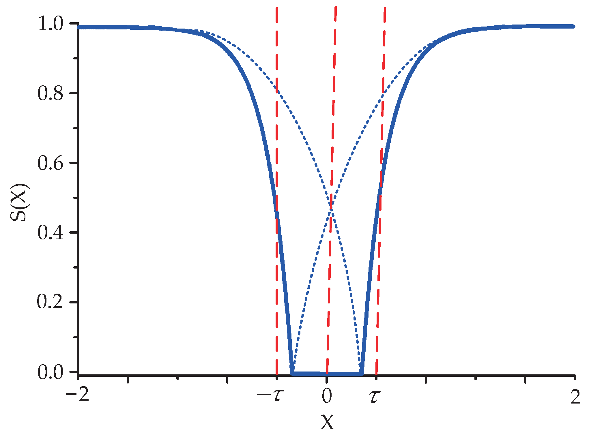
where τ is the scale parameter taken as 0.5, τ is the control limit threshold that must be greater than zero taken as τ = 1 N i = 1 N x ( i ) . The sparsity factor is shown in Figure 4.
Additionally, the wavelet sparse representation of θ ^ 21 is a set of wavelet coefficient vectors. Then, the random matrix X is constructed, obeying Gaussian distribution, θ ^ 2 is measured to obtain the measurement y = X θ ^ 2 , the measurement y is reconstructed to obtain the wavelet coefficients using the orthogonal matching tracking algorithm and the wavelet inverse transform is performed to obtain the recovered signal x ^ .

3.2. Resonant Sparse Signal Decomposition (RSSD)

In Section 3.1, the acoustic signal was processed into a noise-free reconstructed sparse signal using sparse representation in the wavelet domain, but the denoised fault features are still disturbed by the harmonic information. Based on this, the Resonant Sparse Signal Decomposition (RSSD) method is introduced to decompose and de-resonate the acoustic signal according to the different resonant behaviors of high and low frequencies, whereby the fault information is present in the lower resonant components.
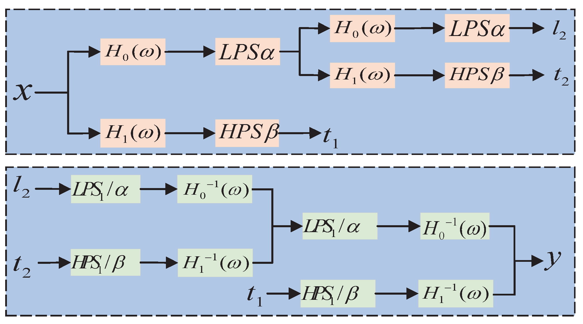
In the RSSD method, two adjustable Q-wavelet transforms ( TQWT ) can be used to represent the signal components of the oscillatory behavior in two different messages, with Q representing the quality factor. It actually represents a two-channel bandpass filter with a real-valued scale factor for signal splitting and filtering as well as synthesis, as schematically shown in Figure 5. While the low-pass filter H 0 ( ω ) and the high-pass filter H 1 ( ω ) are constructed with the following equations [47]:
H 0 ( ω ) = 1 ω ( 1 β ) π θ ω + ( β 1 ) π α + β 1 1 β π ω < α π 0 α π ω < π
H 1 ( ω ) = 0 ω ( 1 β ) π θ α π ω α + β 1 1 β π ω < α π 1 α π ω < π
where the θ function represents the high and low bandpass filter determinants, α and β represent the scaling parameter pair and r represents the redundant oversampling rate. Additionally, the result of TQWT depends on the choice of quality factor, whose maximum decomposition level L m a x can be expressed as [25]
L m a x = l o g ( N 4 Q + 1 ) l o g ( Q + 1 Q + 1 2 r )
The parameters in the RSSD method can be adaptively selected to ensure that their conversion metrics are maximized.

3.3. Analog Signal Processing

To illustrate the effectiveness of the method for acoustic signals, simulated rolling bearing failure acoustic signals from mechanical equipment were used. The signal is expressed as x = x 1 ( t ) + x 2 ( t ) + x 3 ( t ) , and the Doppler distortion effect can be removed directly. The parameters of the simulated signal are shown in Table 1. We know that the signal generated by fault collision is due to transient shock, and when simulating the synthetic signal of a rolling bearing fault, noise and periodic interference harmonic components must be added. Therefore, x 1 ( t ) represents the harmonic component of the period, x 2 ( t ) represents the impact of a rolling bearing failure and x 3 ( t ) indicates the surrounding sound component when the rolling bearing is generated, i.e., noise. In addition, white noise is not considered in the signal to more closely resemble the sound signal in the train wheel pair driving. The formula construction is shown below [48,49]. The time of the simulation signal was set to 0.5 s and the sampling frequency was 45,600 Hz.
x ( t ) = x 1 ( t ) + x 2 ( t ) + x 3 ( t ) x 1 ( t ) = l A l c o s ( 2 π l f r + θ l ) x 2 ( t ) = i C i e 2 π ξ f n ( t i T τ i ) s i n ( 2 π 1 ξ 2 f n ( 2 π ξ f n ( t i T τ i ) + φ 0 ) ) x 3 ( t ) = j R j e 2 π ξ f n ( t T r j ) s i n ( 2 π 1 ξ 2 f n ( t T r j ) )
where f r , A l , θ l are the rotation frequency, amplitude and initial phase of the shaft, respectively. C i , ξ , f n , T , φ 0 denotes the amplitude, damping ratio, intrinsic frequency, period and initial phase, respectively. The bearing fault induction frequency is set to 85 Hz. The time interval is T = 1 / 85 . ξ , R j , f n , T r j . All can be generated by random variables.
Figure 6 shows the simulated generated acoustic signal and the time domain waveform denoised using the wavelet domain Sparse Representation method. Figure 6a is the synthesized simulated signal, Figure 6b is the noise, Figure 6c is the fault signal and Figure 6d is the partial harmonic and the presence of periodic harmonics. According to Equations (12)–(14), the length of the filter was chosen to be 500, the analog acoustic signal was reconstructed by the first wavelet decomposition for sparse representation and a random matrix obeying Gaussian distribution was constructed. After the second wavelet decomposition and inverse wavelet transform, the noise information in the recovered signal is evidently a more sparse signal, indicating that the noise is suppressed. According to the Rasch transform, the control threshold τ > 0 and τ are taken to be close to 2 2 .
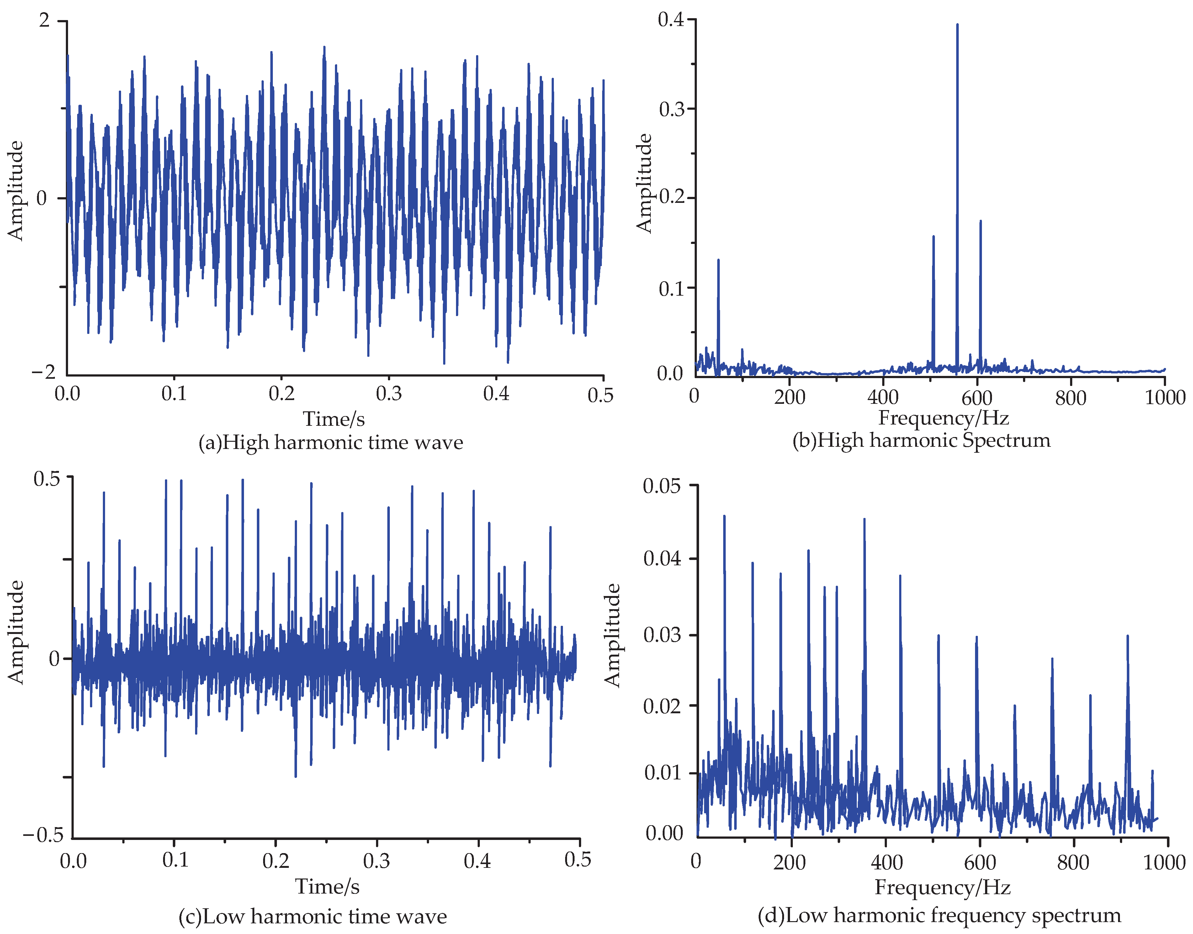
After removing the noise from the signal using wavelet domain Sparse Representation, the fault characteristics may still be disturbed by harmonics since the high- and low-resonance harmonics are composed of different signals and the fault information is found in the lower-harmonic components. Therefore, the RSSD method was introduced in this paper. In order to set the quality factors according to the different signal characteristics, Q 1 and Q 2 were chosen in steps of 0.3 in the range of 4–9 and 1–2, respectively, and the redundancy factor r 3 can reduce the computational effort, so its value was chosen as 3. Combined with Equation (17), the decomposition levels L 1 and L 2 can be determined, which are the maximum decomposition levels for the high and low harmonics, respectively. Figure 7 shows the decomposition of the high- and low-resonance harmonics of the denoised acoustic signal using RSSD. The interference signals present in the high-resonance harmonics are clearly singled out.

4. GA-RBFNN Diagnostic Model

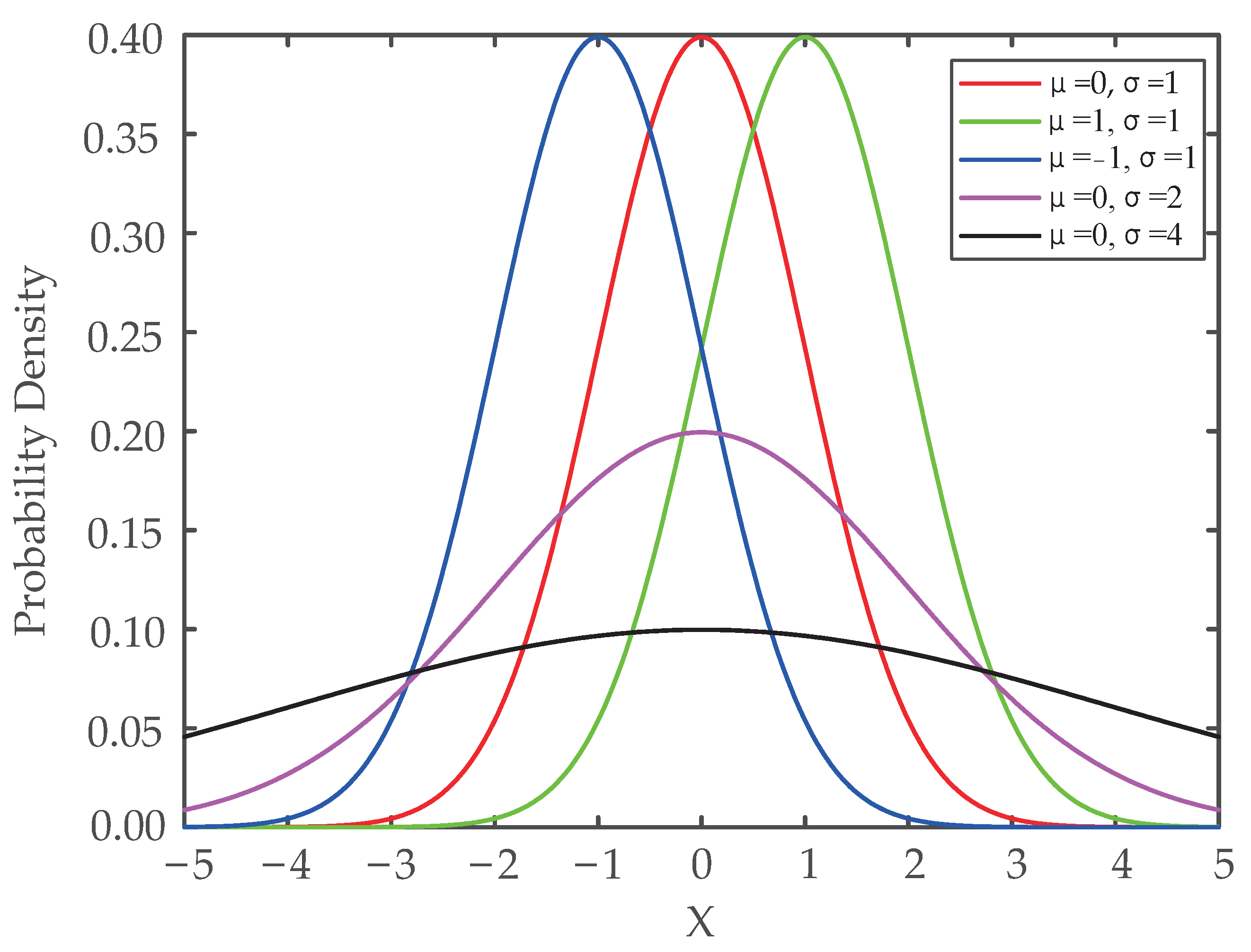
In Section 2.3, the radial basis neural network was defined as a kind of forward propagation neural network with a single hidden layer, possessing a relatively simple network structure but with fast computation speed when computing large data samples. Combined with this paper, a total of four types of faults were designed to be included in the train wheelset bearing: bearing health, inner ring fault, outer ring fault and rolling element fault. The output side of the network only needs to set one output node to satisfy the conditions. However, the RBF neural network regularization requires the determination of three parameters: the center of the function C i , the variance d i and the weights between the hidden layer and the output layer ω k j , where the choice of the variance affects the overall width and computational speed of the network; a comparison graph of the different variances is shown in Figure 8. The mean value of the regularized Gaussian function is μ = ( 0 , 1 , 1 , 0 , 0 ) and the variance is σ 2 = ( 1 , 1 , 1 , 2 , 4 ) . The choice of these three parameters can be determined according to the data to be processed and the optimization method. The roadside acoustic signal feature vector in the diagnosis process contains a large amount of data and requires fast computation, and the GA meets these optimization conditions.
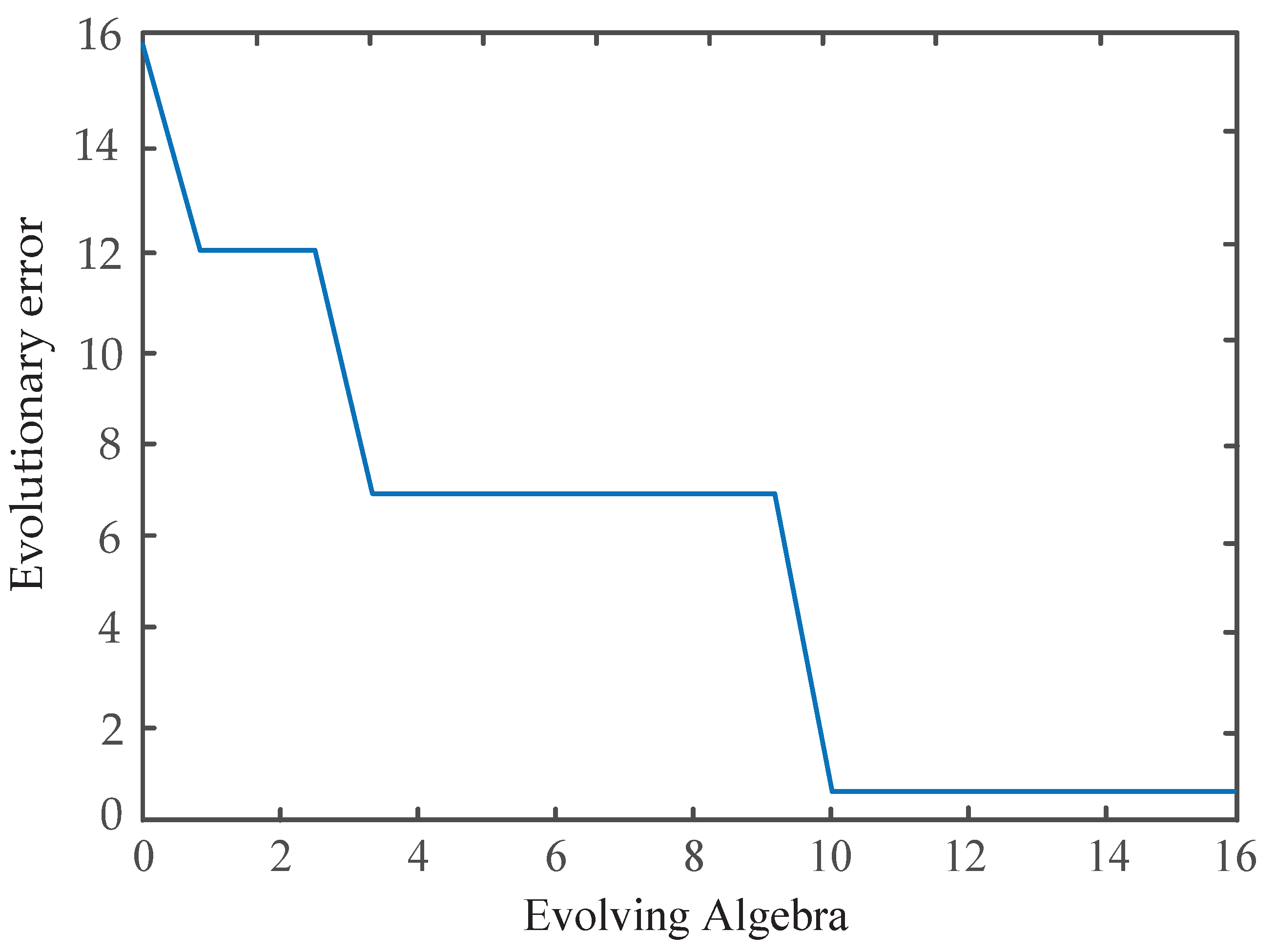
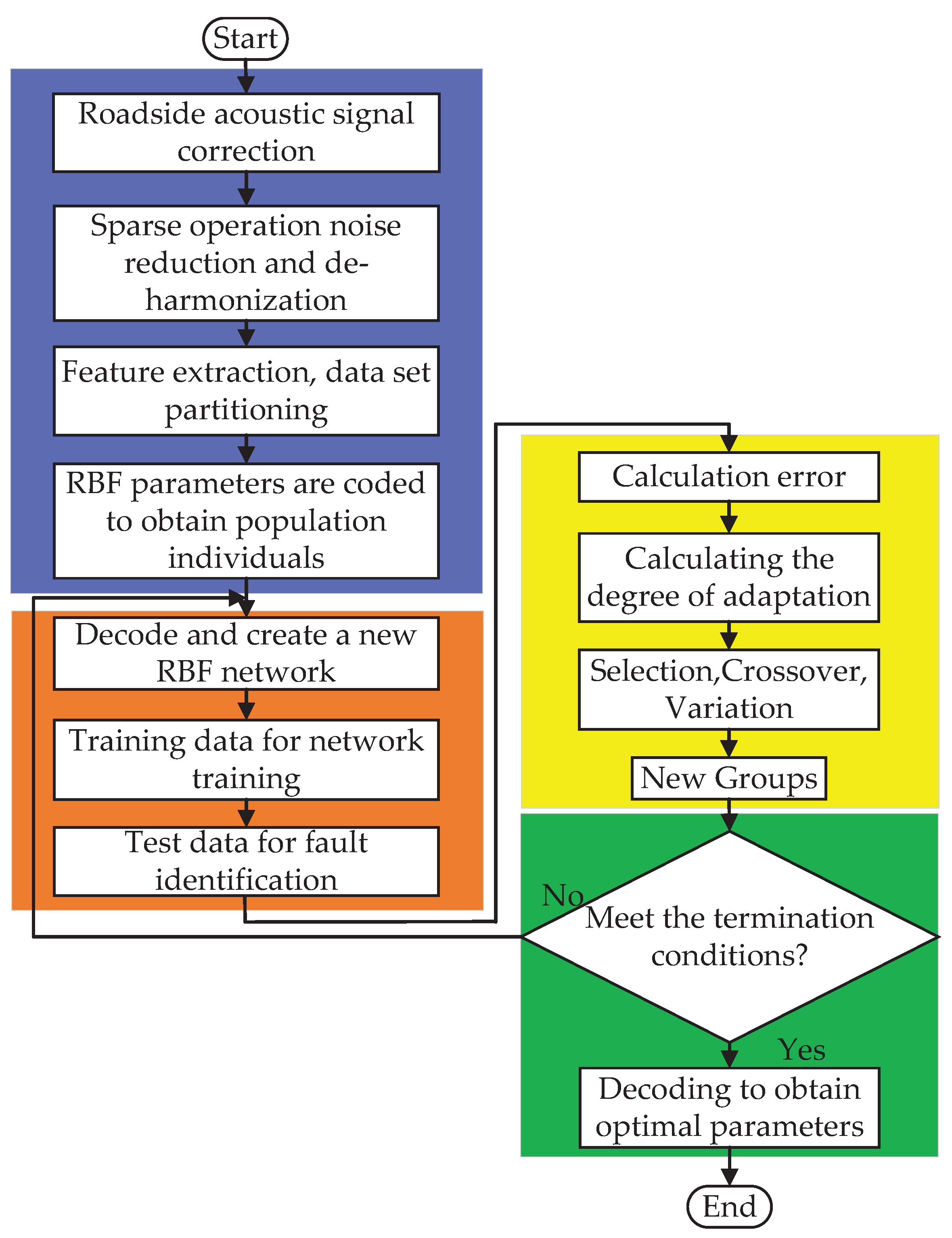
The population individuals of the GA are decided according to the simple structure of the RBF network and the types of faults addressed. The initial population individuals were 60, the maximum number of iterations was 16, the crossover was a two-point crossover to meet the demand, the probability of the crossover was 0.5 and the probability of variation was 0.04. Figure 9 clearly shows when the fitness function is chosen for the misclassification training data, the number of iterations and the evolutionary error variation curve. Figure 10 shows the entire GA-RBF optimization diagnosis process.

5. Experimental Signal Analysis

5.1. Experimental Conditions

In order to verify the effectiveness of the proposed method, the acoustic signals collected by the TADS diagnostic system in service along a railroad section in China were selected for verification, and the acoustic signals were the original signals not transformed into electrical signals after the system was collected. The acoustic acquisition of the train wheelset bearings is shown schematically in Figure 11. A train was recorded three times through the collection system, measuring when the alarm was triggered by the wheelset bearing position of an abnormal acoustic wave in the same carriage and on the same side. Eventually, after inspection of the wheel pair disassembly process, it was clear that the wheel pair bearing contained faults such as damage to the outer ring, inner ring and rolling body, and the fault level was determined to be a secondary fault, with the wheel pair bearing fault location shown in Figure 12. That is, the recorded sound can be determined to be the fault signal, which can be used as the main signal for the next analysis.
After the staff measurement, the damage data size is shown in Table 2. At the same time, the acquisition of the train’s into- and out-of-speed comparison and access to the shaft temperature detection system and humidity test were measured, the resulting data of which are shown in Table 3. It is worth noting that the temperature here for the adhesion of the bearing temperature sensor, a temperature change control of 80 ° C or less, indicates that the temperature is not abnormal; furthermore, the humidity can only be taken as a relative value, with acquisition of the humidity sensor below 70%, indicating that there is also no major change. In addition, it can be seen that the speed of the train passing through the acquisition system does not vary by much, so there is no significant change in speed nor in the temperature or humidity values, thus having a minimal impact on the acoustic signal and not affecting the quality of the signal itself.
When the train passes through the collection system, the speed is 90 km/h–120 km/h; at this time, the axial load of the bearing is 6 t; the speed is 9050 r/min; the sampling frequency is 48 kHz; the sampling depth is 24 bits; and the vertical distance from the train’s wheel-to-wheel sound source is r = 2 m. Additionally, it is known that the bearing is a single-row radial cylindrical roller bearing (NU2234U), commonly used in China, and its parameters are shown in Table 4.
According to the acoustic files collected by the train trackside acoustic signal acquisition system, the three types of wheelset bearings contain fault acoustic signals. Each type of collected acoustic signal is rounded to 12 s, and the healthy bearing acoustic signals of different locations and times of the same train are randomly collected and rounded to 12 s to facilitate the subsequent data processing and feature extraction.

5.2. Roadside Acoustic Signal Sparse Operation

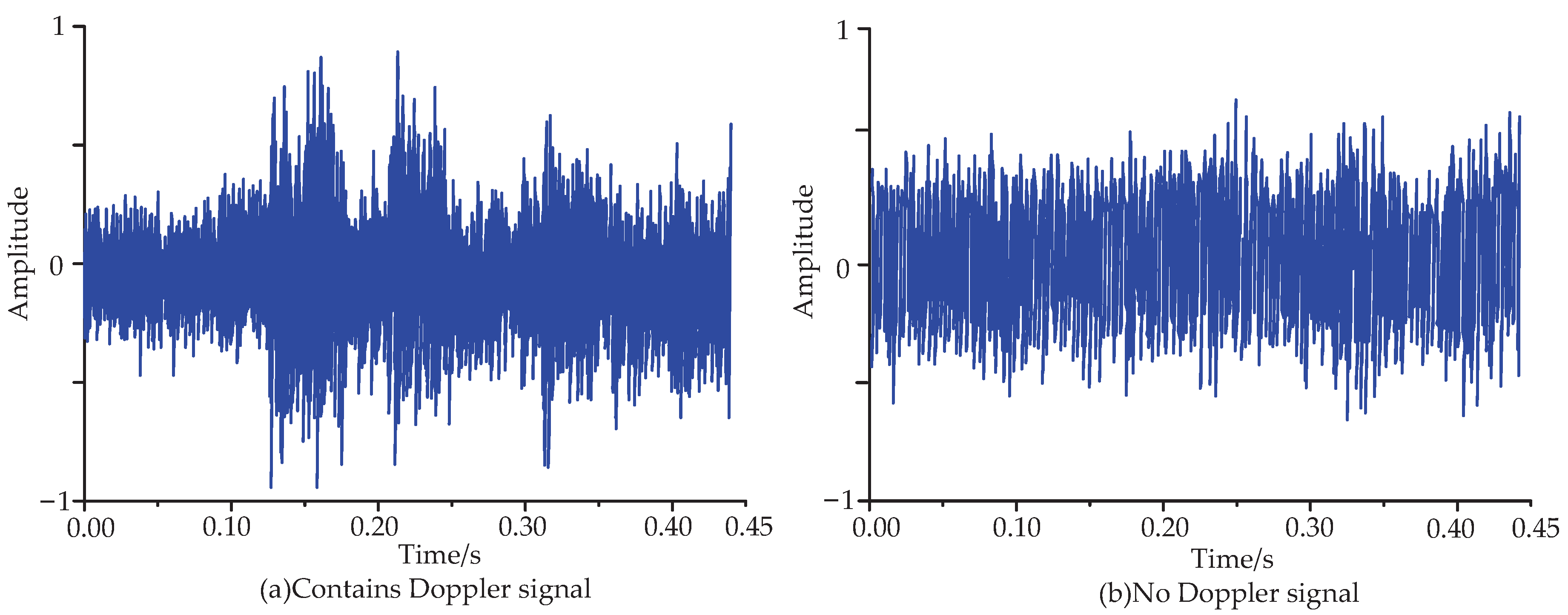
For the acquired channel-side acoustic signals, the TIR technique was used for Doppler aberration correction, and it can be seen that most of the offset waveforms were corrected, as shown in Figure 13, for the outer ring fault signal.
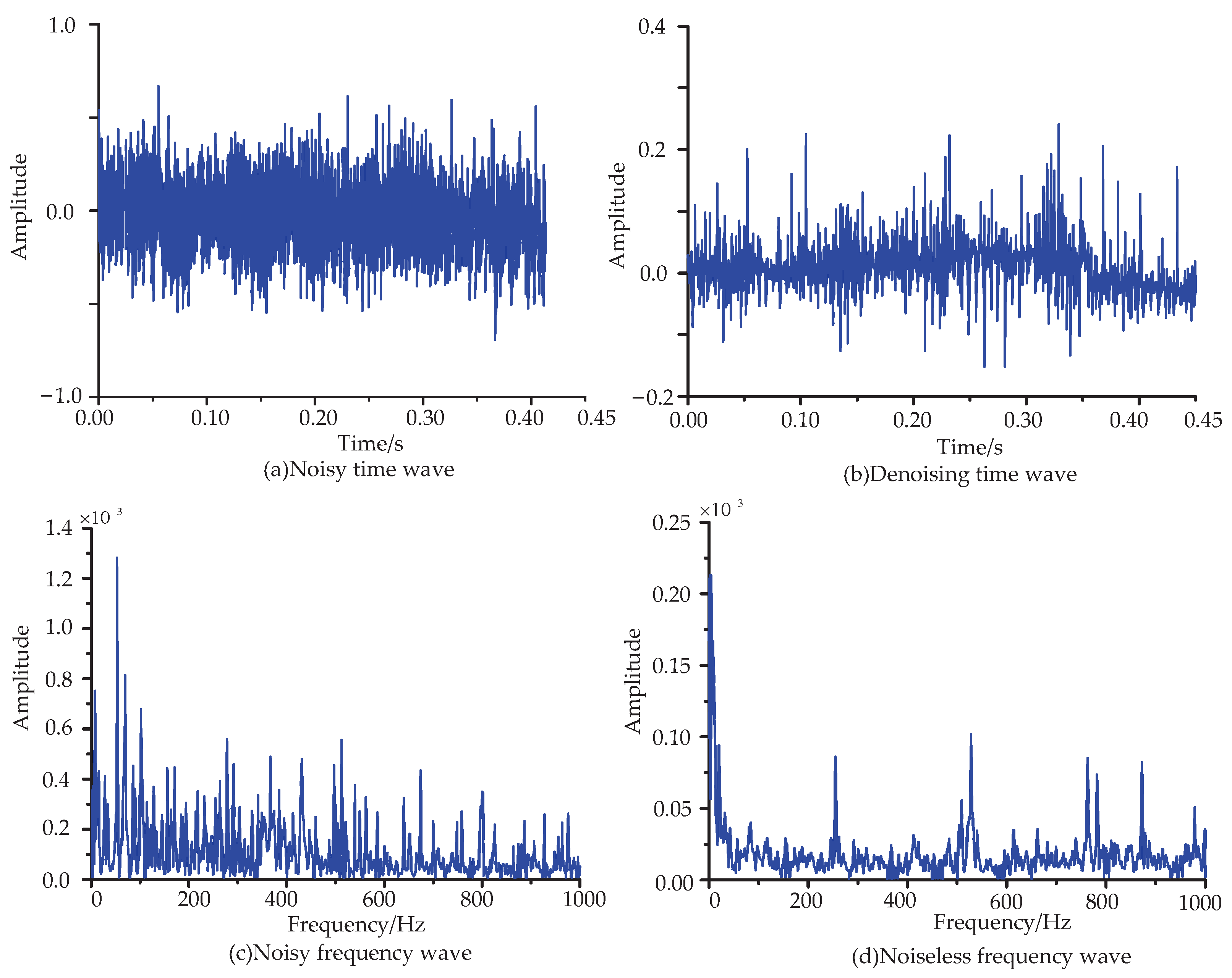
The wavelet domain sparse representation of the Doppler-free acoustic signal is denoised with a correction signal of 0.45 s per segment, a hard threshold of 1 for the adaptive filter and a sparsity factor of τ = 0.5 . The time–frequency domain waveforms after denoising are shown in Figure 14a,b, which is the time domain waveform, and Figure 14c,d, which is the frequency domain waveform.
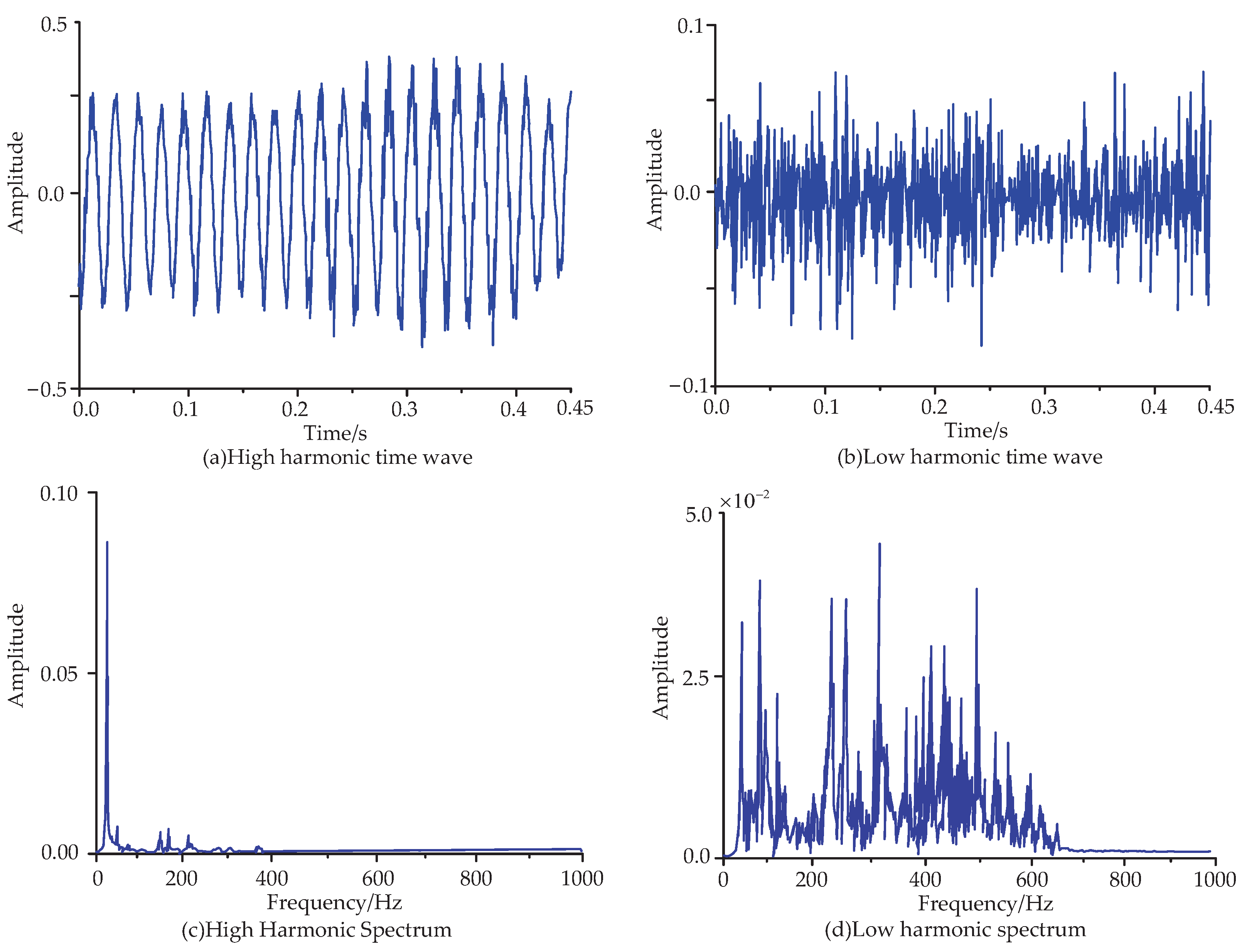
The sound waveform after noise reduction clearly shows the coexistence of high- and low-resonance harmonics, and the fault information is in the low-resonance harmonics. The RSSD further removes the interference harmonics, as shown in Figure 15.
In Figure 15a,c are high-resonance harmonics and Figure 15b,d are low-resonance harmonic signals containing fault information. To compare and illustrate the effectiveness of this method, the commonly used VMD method was used, and the maximum kurtosis-worthy IMF was chosen. It is evident from Figure 16 that f exists, indicating the presence of interference harmonics, making it evidently inferior to the RSSD method.

5.3. Feature Extraction

From the roadside sound signals acquired, the TADS system collected four types of sound signals: health signal, outer ring fault signal, inner ring fault signal and rolling body fault signal. Each type of signal comprises 10 samples, with a total of 40 samples wherein each type of signal taken is a 12 s sound file, using wavelet domain Sparse Representation for noise reduction and RSSD to remove interference harmonics, and then cut into 0.4 s sections of sound samples, totaling 1200 samples.
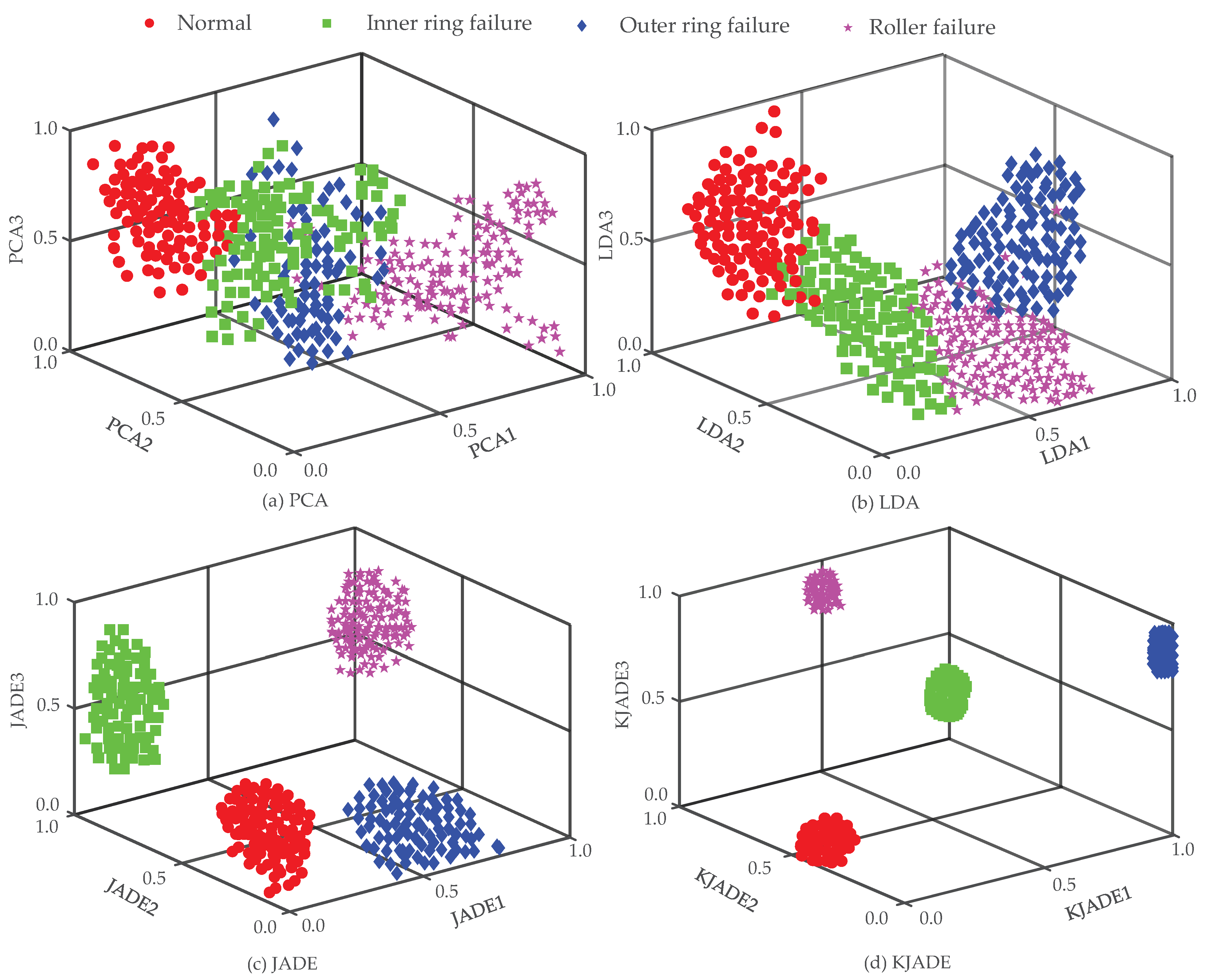
These data are then divided into a training set and a test set. Ten original statistical features were extracted for each signal class according to Table 5 to obtain the sample vectors of the four states of the train wheel pair bearings. The extracted time–frequency domain features were fused and clustered using the KJADE algorithm [50]. The convenient input into the GA-RBFNN caused data confusion due to the feature set; therefore, to increase the comparability, the PCA algorithm, LDA fusion algorithm and JADE algorithm were selected after these features were reduced to the three-dimensional space for T-SNE visualization. The comparison results are shown in Figure 17a,b, which show the clustering effect, but there is still feature-scattered adhesion [50]; Figure 17c shows that, although the clustering effect is evident, the clustering effect of single features is not good [50]; and Figure 17d shows that the clustering of the four types of features is very good [50], with the features of each signal having their own clustering centers, indicating that the selected feature fusion algorithm clustering effect is superior. The number of training samples for the processed signals was set to 60 groups of 240 samples per class for a total of 960 samples, and the test samples were set to 15 groups of 60 samples per class for a total of 240 samples.

5.4. Analysis of the GA-RBFNN Diagnostic Results

From Section 5.1 and Section 5.2, the training data and test data were cut into a total of 300 groups, of which 240 groups comprised the training data and 60 groups comprised the bearing health status, inner ring failure, outer ring failure and rolling element failure each, with labels set to 1, 2, 3 and 4, respectively. Fifteen groups were available for the rolling bearing status of each wheel pair in the test data. The training samples were input into the default parameters in RBFNN and GA-RBFNN, and their training results were compared, as shown in Figure 18. The training samples were input into the RBFNN with default parameters and the RBFNN optimized with GA parameters. It is evident that both are essentially the same in terms of the number of iterations, and that the basic training error remains the same after 22 iterations; however, the GA-RBFNN training error is closer to the target 0 compared to the RBFNN with default parameters. Therefore, comparing the two curves proves that the RBFNN has a stronger convergence after GA optimization.
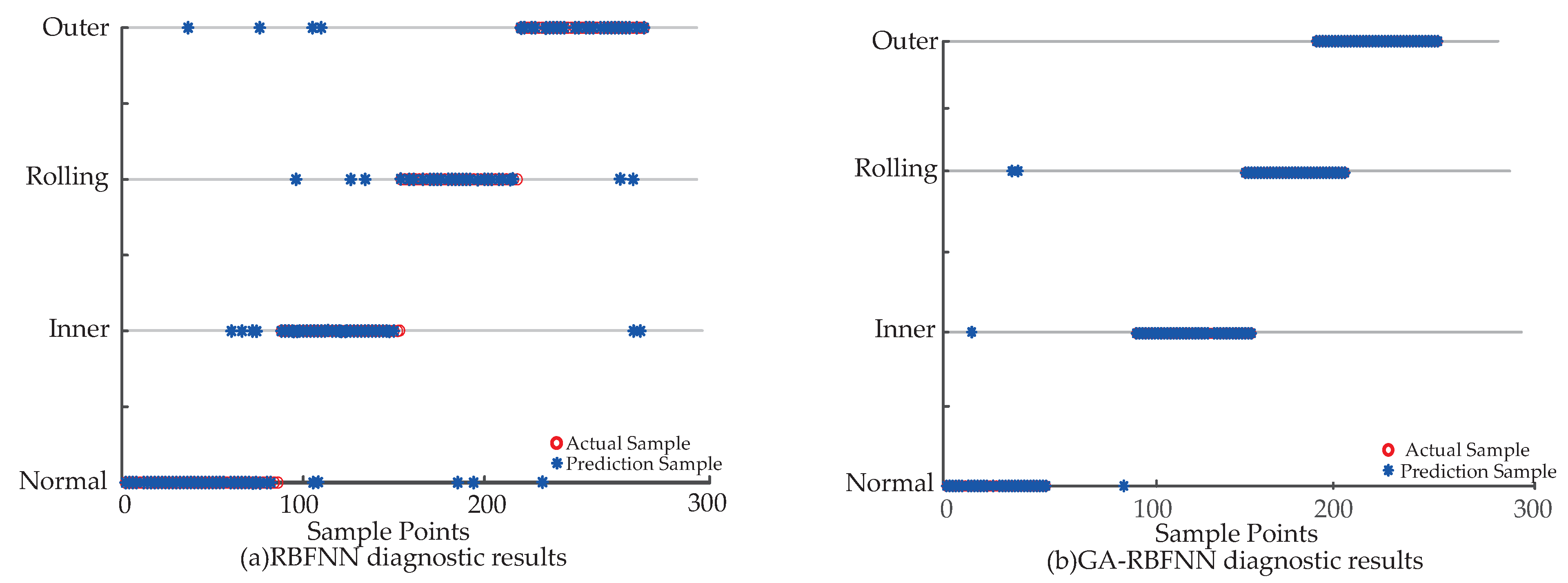
The processed training and test data were then input into the RBNN with default parameters and the RBNN optimized using the GA to perform fault diagnosis of the four types of acoustic signals of the train wheelset rolling bearings. The output results of the fault diagnosis are shown in Figure 19, Figure 20, Figure 21 and Figure 22.
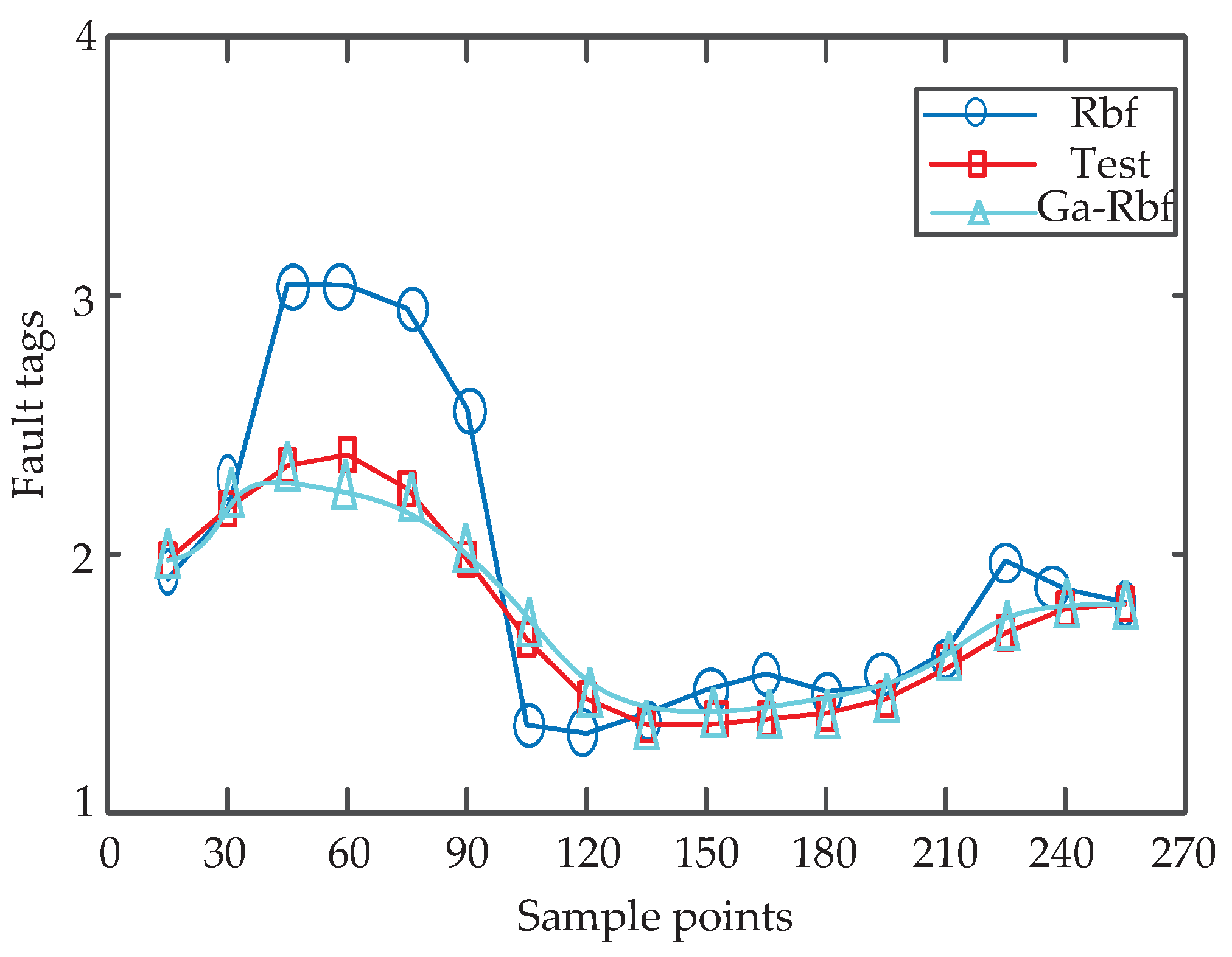
As seen in Figure 19, there are nearly 20 incorrect test data elements in the RBNN diagnostic results with the default parameters, with each set of data set to three sets of sample points averaged over each type of fault data, totaling 300 sets of data. The diagnostic accuracy of the default neural network is only 79.6%. In the test data plot after the GA optimization, it can be seen that there are four data points that fail to fit accurately, and the diagnosis accuracy reaches 97.22% when averaged over 300 sets of data. The GA-optimized RBFNN test data fit the training data better, as can be seen in Figure 20 and Figure 21. After the confusion matrix, it can be seen that the diagnosis rate of the rolling body and normal bearing among the four types of fault signals is 100%, and that the latter improved the accuracy rate by an extra 18% compared with the former, proving the effectiveness of the GA-optimized radial base acoustic feature fault identification network.
To further compare and illustrate the effectiveness of the method, the acoustic feature data in Section 5.3 were input into the SVM, BP neural network, GA-SVM and GA-BPNN for training and testing, and the recognition accuracy and rate of each classifier are shown in Table 6. Combined with Figure 22, it can be clearly seen that the GA-BPNN is closer to the GA-RBFNN in recognition accuracy. However, its recognition rate is significantly slower because its BP network structure is more complex than RBF. It can also be seen that the recognition accuracy of GA-SVM, which has a faster recognition rate than GA-RBFNN, is much lower and cannot be used for fault diagnosis. In summary, the fault diagnosis model of the GA-RBFNN roadside acoustic signal is superior to some traditional fault diagnosis models.

6. Conclusions

  • For the processing of the background noise and interference harmonics in roadside acoustic signals, this paper creatively utilizes the sparse representation method in the wavelet domain to completely remove the powerful reverberation noise in the roadside acoustic signal, while using the RSSD method to remove the interference harmonics, laying the foundation to be able to smoothly extract the features and the fault diagnosis of acoustic signals.
  • For the premise of low-efficiency fault identification in roadside acoustic signals and less-researched methods, a GA-RBFNN model of roadside acoustic fault feature diagnosis was proposed. Using the characteristics of GA’s adaptability to large data processing and robustness, and RBNN’s simple structure and fast processing speed, the simulation experiments of TADS fault acoustic data in a railroad section site prove that, after a variety of time–frequency domain fusion clustering acoustic feature vector inputs, the model can achieve fast and accurate identification of the fault type, with a recognition accuracy as high as 97.22%. The superiority of the method is comprehensively demonstrated when comparing the diagnosis rate and accuracy with those of other diagnosis models.

Author Contributions

Conceptualization, J.Q.; Data curation, J.R.; Formal analysis, J.R., F.Y. and Q.Z.; Funding acquisition, J.Q. and M.T.; Investigation, J.R., M.T., F.Y. and Q.Z.; Methodology, J.Q., M.T. and J.R.; Project administration, J.Q.; Resources, J.Q. and F.Y.; Software, J.R.; Supervision, J.Q. and M.T.; Validation, M.T., F.Y. and Q.Z.; Visualization, J.R. and M.T.; Writing—original draft, J.Q. and J.R.; Writing—review and editing, J.Q. and M.T. All authors have read and agreed to the published version of the manuscript.

Funding

This research was funded by National Natural Science Foundation of China Grant Program, grant numbers (61663021, 61763025, 61861025).

Institutional Review Board Statement

Not applicable.

Informed Consent Statement

Not applicable.

Data Availability Statement

Not applicable.

Acknowledgments

The authors gratefully acknowledge the support they received from the National Natural Science Foundation of China Grant Program (61663021, 61763025, 61861025).

Conflicts of Interest

The authors declare no conflict of interest. The funders had no role in the design of the study; in the collection, analyses, or interpretation of data; in the writing of the manuscript; or in the decision to publish the results.

References

  1. Cai, Q.H.; Peng, H.M. Bearings for railroad vehicles. Foreign Locomot. Roll. Stock. Technol. 2010, 2, 17–20. [Google Scholar]
  2. Qiao, Z.C.; Liu, Y.Q.; Liao, Y.Y. Application of improved MOMEDA method based on Teager energy operator in railroad wheelset bearing fault diagnosis. Bearing 2020, 4, 43–50. [Google Scholar]
  3. Cai, Y.; Lin, J.H.; Zhang, W.H.; Ding, J.M. Faults diagnostics of railway axle bearings based on IMF’s confidence index algorithm for ensemble EMD. Sensors 2015, 15, 10991–11011. [Google Scholar] [CrossRef] [PubMed] [Green Version]
  4. Li, X.M.; He, D.Q.; Tan, W.J.; Chen, E.H. Research on rolling bearing fault diagnosis of trains based on EEMD and RBFNN. J. Railw. Sci. Eng. 2017, 14, 1056–1062. [Google Scholar]
  5. Deng, F.Y.; Ding, H.; Lv, H.Y.; Hao, R.J.; Liu, Y.Q. A lightweight neural network-based fault diagnosis method for high-speed railway wheelset bearings. Chin. J. Eng. 2021, 43, 1482–1490. [Google Scholar]
  6. Miao, M.Q.; Sun, Y.H.; Yu, J.B. Deep sparse representation network for feature learning of vibration signals and its application in gearbox fault diagnosis. Knowl.-Based Syst. 2022, 240, 108116. [Google Scholar] [CrossRef]
  7. Li, H.K.; Wei, Y.Q.; Yang, G. A review of research on trackside acoustic fault diagnosis of rolling stock bearings. Bearing 2022, 11, 1–7. [Google Scholar]
  8. Zhang, S.B.; Zhang, H.B.; OuYang, K.S.; He, Q.B.; Kong, F.R. Doppler correction method for train bearing fault acoustic signals based on time-frequency amplitude matching. J. Vib. Shock 2016, 35, 101–106. [Google Scholar]
  9. Liu, F.; He, Q.B.; Shen, C.Q.; Hu, F.; Zhang, A.; Kong, F.R. A time-domain correction method for Doppler distortion signals of moving sound sources. Sheng Hsueh Hsueh Pao Acta Acust. 2014, 39, 185–190. [Google Scholar]
  10. Wu, Q.; He, Q.B.; Kong, F.R. Doppler distortion correction of roadside acoustic signals. J. Data Acquis. Process. 2014, 29, 309–315. [Google Scholar]
  11. Yuan, Z.Z.; Kong, F.R.; Zhang, H.B.; Hu, F.; Liu, F.; Zhu, P.L. A Doppler distortion acoustic signal correction method based on instantaneous frequency. Mach. Electron. 2013, 12, 36–39. [Google Scholar]
  12. Wu, Q.; Kong, F.R.; He, Q.B.; Liu, Y.B. Doppler distortion correction of acoustic signals based on resampling technique. J. Process. 2012, 28, 1308–1313. [Google Scholar]
  13. Ding, X.X.; Li, Y.L.; Xiao, J.W.; He, Q.B.; Yang, X.Q.; Shao, Y.M. Parametric Doppler correction analysis for wayside acoustic bearing fault diagnosis. Mech. Syst. Signal Process. 2022, 166, 108375. [Google Scholar] [CrossRef]
  14. Bi, C.X.; Li, Y.C.; Zhang, Y.B.; Zhang, X.Z.; Xu, L. Signal reconstruction of moving sound sources with a fixed microphone array. Mech. Syst. Signal Process. 2019, 118, 277–289. [Google Scholar] [CrossRef]
  15. Amarnath, M.; Krishna, I.P. Empirical mode decomposition of acoustic signals for diagnosis of faults in gears and rolling element bearings. IET Sci. Meas. Technol. 2012, 6, 279–287. [Google Scholar] [CrossRef]
  16. Zhang, J.Q.; Chen, Y.G.; Li, N.; Zhai, J.Y.; Han, Q.K.; Hou, Z.X. A Denoising Method of Micro-Turbine Acoustic Pressure Signal Based on CEEMDAN and Improved Variable Step-Size NLMS Algorithm. Machines 2022, 10, 444. [Google Scholar] [CrossRef]
  17. Lv, X. Advances in high performance acoustic filter technology. Digit. Design 2021, 4, 10. [Google Scholar]
  18. Liu, F.; Zhao, X.H.; Zhu, Z.H.; Zhai, Z.P.; Liu, Y.B. Dual-microphone active noise cancellation paved with Doppler assimilation for TADS. Mech. Syst. Signal Process. 2023, 184, 109727. [Google Scholar] [CrossRef]
  19. Xiao, D.Y.; Qin, C.J.; Yu, H.G.; Huang, Y.X.; Liu, C.L.; Zhang, J.W. Unsupervised machine fault diagnosis for noisy domain adaptation using marginal denoising autoencoder based on acoustic signals. Measurement 2021, 176, 109186. [Google Scholar] [CrossRef]
  20. Sun, Y.; Yuan, M.; Feng, H.H. A statistical model-based improved spectral noise reduction algorithm. Acoust. Tech. 2013, 32, 115–118. [Google Scholar]
  21. Niall, H.; Rickard, S. Comparing measures of sparsity. IEEE Trans. Inform. Theory 2009, 55, 4723–4741. [Google Scholar]
  22. Martin, G.; Kutyniok, G.; März, M. 1-analysis minimization and generalized (co-) sparsity: When does recovery succeed? Appl. Comput. Harm. Anal. 2021, 52, 82–140. [Google Scholar]
  23. Zhang, Z.R.; Wang, J.R.; Li, S.M.; Han, B.K.; Jiang, X.X. Fast nonlinear blind deconvolution for rotating machinery fault diagnosis. Mech. Syst. Signal Process. 2023, 187, 109918. [Google Scholar] [CrossRef]
  24. Hou, Y.C.; Zhou, C.Q.; Tian, C.M.; Wang, D.; He, W.T.; Huang, W.J.; Wu, P.; Wu, D.Q. Acoustic feature enhancement in rolling bearing fault diagnosis using sparsity-oriented multipoint optimal minimum entropy deconvolution adjusted method. Appl. Acoust. 2022, 201, 109105. [Google Scholar] [CrossRef]
  25. Yu, G.Y.; Ge, Y.; Ma, B. Feature enhancement method of rolling bearing acoustic signal based on RLS-RSSD. Measurement 2022, 192, 110883. [Google Scholar] [CrossRef]
  26. Zhang, D.C.; Xie, M.; Hamadache, M.; Entezami, M.; Stewart, E. An adaptive graph morlet wavelet transform for railway wayside acoustic detection. J. Sound Vib. 2022, 529, 116965. [Google Scholar] [CrossRef]
  27. Glowacz, A. Acoustic fault analysis of three commutator motors. Mech. Syst. Signal Process. 2019, 133, 106226. [Google Scholar] [CrossRef]
  28. Glowacz, A.; Glowacz, W.; Glowacz, Z.; Kozik, J. Early fault diagnosis of bearing and stator faults of the single-phase induction motor using acoustic signals. Measurement 2018, 113, 1–9. [Google Scholar] [CrossRef]
  29. Lu, W.B.; Jiang, W.K.; Wu, H.J.; Hou, J.J. A fault diagnosis scheme of rolling element bearing based on near-field acoustic holography and gray level co-occurrence matrix. J. Sound Vib. 2012, 331, 3663–3774. [Google Scholar] [CrossRef]
  30. Lu, W.B.; Jiang, W.K.; Yuan, G.Q.; Li, Y. A gearbox fault diagnosis scheme based on near-field acoustic holography and spatial distribution features of sound field. J. Sound Vib. 2013, 332, 2593–2610. [Google Scholar] [CrossRef]
  31. Zhang, D.C.; Entezami, M.; Stewart, E.; Roberts, C.; Yu, D.J. Intelligent acoustic-based fault diagnosis of roller bearings using a deep graph convolutional network. Measurement 2020, 156, 107585. [Google Scholar] [CrossRef]
  32. Yang, J.M.; Zhou, W.J.; Song, T.X. Audio-based fault diagnosis for belt conveyor rollers. Neurocomputing 2020, 397, 447–456. [Google Scholar] [CrossRef]
  33. Wang, J.J.; Yang, S.P.; Liu, Y.Q.; Gui, L.W. Deep Subdomain Transfer Learning with Spatial Attention ConvLSTM Network for Fault Diagnosis of Wheelset Bearing in High-Speed Trains. Machines 2023, 11, 304. [Google Scholar] [CrossRef]
  34. Li, S.B.; Yao, Y.; Gui, G.; Li, X.; Hu, J.J. Gear fault diagnosis based on CNN and multi-channel acoustic signal. China Meas. Test. 2019, 45, 1–5. [Google Scholar]
  35. Yu, L.J.; Wang, R.; Liu, F.K. Acoustic Fault Diagnosis of Rolling Bearings Based on Blending Model Fusion of Multiple Convolutional Neural Network. Fail. Anal. Prev. 2021, 16, 238–245. [Google Scholar]
  36. Hasan, M.J.; Islam, M.M.M.; Kim, J.M. Acoustic spectral imaging and transfer learning for reliable bearing fault diagnosis under variable speed conditions. Measurement 2019, 138, 620–631. [Google Scholar] [CrossRef]
  37. Liu, Y.J.; Chen, B.F.; Ding, L.P. Fault diagnosis method of micro-motor based on acoustic features. March. Build. Automa 2022, 51, 190–194. [Google Scholar]
  38. Yao, Y.; Gui, G.; Yang, S.X.; Zhang, S. A Recursive Denoising Learning for Gear Fault Diagnosis Based on Acoustic Signal in Real Industrial Noise Condition. IEEE Trans. Instrum. Meas. 2021, 70, 1–15. [Google Scholar] [CrossRef]
  39. Ji, S.S.; Han, B.K.; Zhang, Z.Z.; Wang, J.R.; Lu, B.; Yang, J.W.; Jiang, X.X. Parallel sparse filtering for intelligent fault diagnosis using acoustic signal processing. Neurocomputing 2021, 462, 466–477. [Google Scholar] [CrossRef]
  40. Ntalampiras, S. One-shot learning for acoustic diagnosis of industrial machines. Expert Syst. Appl. 2021, 178, 114984. [Google Scholar] [CrossRef]
  41. Xu, T.; Wang, H.J. Rolling bearing fault diagnosis based on VMD transient energy and GA-RBF. J. Railw. Sci. Eng. 2020, 2, 74–78. [Google Scholar]
  42. Klinaku, S. The Doppler effect is the same for both optics and acoustics. Optik 2021, 244, 167565. [Google Scholar] [CrossRef]
  43. Fan, H.; Guo, P.; Wang, F.m. Research development of sparse representation of non-stationary signals. Comput. Eng. Appl. 2012, 1, 278–284. [Google Scholar]
  44. Liu, Y.; Zhang, L.Y. Implementation of BP and RBF neural networks and their performance comparison. Electr. Measur Tech. 2007, 30, 77–80. [Google Scholar]
  45. Qiu, J.D.; Jiang, Z.Y. Research on railroad freight volume forecasting based on NLAPSO-RBF. Comput. Eng. Appl. 2013, 49, 253–257. [Google Scholar]
  46. Zhao, Z.p.; Ceng, Y.G.; Chen, X.F. Sparse representation of signal based on wavelet-domain Wiener filter. J. Appl Sci. 2012, 30, 595–600. [Google Scholar]
  47. Zhang, D.C.; Entezami, M.; Stewart, E.; Roberts, C.; Yu, D.J. Adaptive fault feature extraction from wayside acoustic signals from train bearings. J. Sound Vib. 2018, 425, 221–238. [Google Scholar] [CrossRef]
  48. Žvokelj, M.; Zupan, S.; Prebil, I. EEMD-based multiscale ICA method for slewing bearing fault detection and diagnosis. J. Sound Vib. 2016, 370, 394–423. [Google Scholar] [CrossRef]
  49. Ni, Q.; Ji, J.C.; Ke, F.; Halkon, E. A fault information-guided variational mode decomposition (FIVMD) method for rolling element bearings diagnosis. Mech. Syst. Signal Process. 2022, 164, 108216. [Google Scholar] [CrossRef]
  50. Long, L.; He, B.; Liu, F.; Liu, Y.B.; Li, G.H.; Lu, S.L. Research on the acoustic diagnosis method of train bearing trackside based on KJADE. J. Vib. Mear. Diagn. 2020, 40, 781–787+828–829. [Google Scholar]
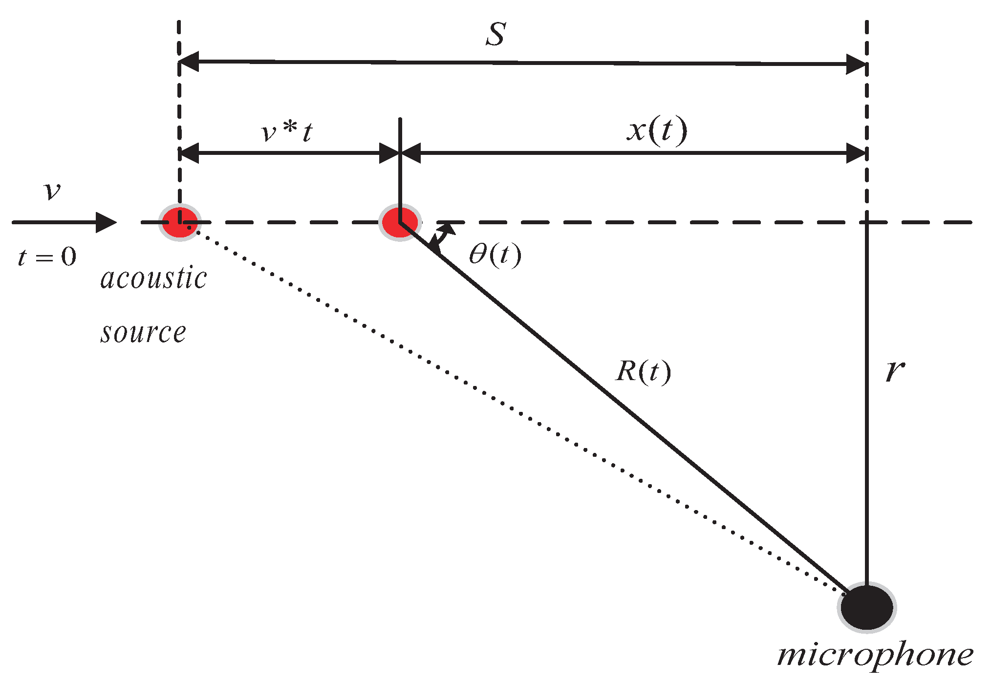
Figure 1. Roadside acoustic acquisition model.
Machines 11 00765 g001
Figure 2. Gaussian topology of radial basis network.
Machines 11 00765 g002
Figure 3. Sparse representation of wavelet domain adaptive filtering.
Machines 11 00765 g003
Figure 4. Design sparsity factor.
Machines 11 00765 g004
Figure 5. TQWT process schematic.
Machines 11 00765 g005
Figure 6. Analog signal denoising results. (a) Displayed as a time-domain graph of the total synthesized signal; (b) Time-domain plot of a noisy signal; (c) Includes time-domain diagram of fault signals; (d) is periodic interference harmonic.
Machines 11 00765 g006
Figure 7. RSSD method for de-noised signals. (a,b) are the time-domain plot and frequency-domain envelope of the highly resonant interference harmonics; (c,d) are the time-domain plot and frequency-domain envelope of the low-resonance interference harmonic.
Machines 11 00765 g007
Figure 8. Gaussian curve distribution with different mean variances.
Machines 11 00765 g008
Figure 9. Evolutionary process of GA-RBFNN.
Machines 11 00765 g009
Figure 10. GA-RBF optimization process.
Machines 11 00765 g010
Figure 11. TADS roadside acoustic signal acquisition map.
Machines 11 00765 g011
Figure 12. Bearing damage position.
Machines 11 00765 g012
Figure 13. Doppler signal correction effect. (a) is time-domain plot of train trackside acoustic signals containing Doppler effect; (b) is time-domain plots of train trackside acoustic signals corrected for Doppler effects.
Machines 11 00765 g013
Figure 14. Experimental signals Wavelet domain sparse representation denoising. (a,c) are time-domain plot and frequency-domain envelope of the noise signal; (b,d) are time-domain plot and frequency-domain envelope after noise removal.
Machines 11 00765 g014
Figure 15. RSSD acoustic signal processing. (a,c) are time-frequency domain effect of demodulated highly resonant interference harmonics; (b,d) are time-frequency domain effects of demodulated low resonance harmonics.
Machines 11 00765 g015
Figure 16. VMD processing comparison graph. (a) is time-domain waveforms of VMD processed signals; (b) is frequency domain envelope of the VMD processed signal.
Machines 11 00765 g016
Figure 17. Comparison of the effectiveness of different feature clustering methods. (a) is the clustering effect of feature groups after PCA treatment; (b) is the clustering effect of feature groups after LDA treatment; (c) is the clustering effect of feature groups after JADE treatment; (d) is the clustering effect of the feature group after the KJADE treatment.
Machines 11 00765 g017
Figure 18. Comparison of GA-RBF iteration curves.
Machines 11 00765 g018
Figure 19. Diagnostic results comparison chart. (a) is the fault recognition effect of RBF neural network with default parameters; (b) is a plot of the fault identification effect of the RBF neural network after using the GA optimization parameters.
Machines 11 00765 g019
Figure 20. Confusion matrix of diagnostic results.
Machines 11 00765 g020
Figure 21. Diagnostic result fitting curve.
Machines 11 00765 g021
Figure 22. Comparison of diagnostic effects of multiple methods.
Machines 11 00765 g022
Table 1. Simulation of bearing channel side acoustic signal parameters.
x 1 ( t ) Rotation
frequency
PhasesAmplitudePhasesAmplitude
  50  90 10  180  5
x 2 ( t ) Rotation
frequency
PeriodicityAmplitudeDamping
ratio
Phases
 4250 1/85 (0,1) 0.03 270
x 3 ( t ) Change
frequency
TimeDamping
ratio
Amplitude\
 ∼U (2000, 6000) ∼U (0,5)0.025 ∼U ( −2,2)\
Table 2. Bearing failure dimensions.
No.Fault LocationFault Point Size (Length × Width × Depth)
1Normal/
2Inner ring failure50 mm × 40 mm × 3 mm
3Outer ring failure50 mm × 50 mm × 3 mm
4Roller failure10 mm × 10 mm × 2 mm
Table 3. Speed temperature and humidity values at the time of acquisition.
SpeedTemperatureHumidity
Drive inDrive out
First95 km/h96 km/h55 °C40%
Second97 km/h96 km/h61 °C47%
Third95 km/h96 km/h53 °C53%
Table 4. NU2234U bearing parameters.
Inner
Diameter
Outer
Diameter
Section Circle
Diameter
Rolling Body
Diameter
Roller
Numbers
170 mm310 mm277 mm58 mm14
Table 5. Original feature extraction.
Time DomainFrequency Domain
F 1 = 1 N i = 1 N x i F 6 = 1 N i = 1 N x i 3
F 2 = 1 N i = 1 N x i 2 F 7 = 1 N i = 1 N x i 2 F 4
F 3 = 1 N i = 1 N x i 2 F 8 = 1 N i = 1 N x i 4 1 N j = 1 N x j 2
F 4 = 1 N i = 1 N x i F 9 = 1 N i = 1 N S i
F 5 = m a x ( x ) 1 N i = 1 N x i F 10 = 1 N j = 1 N ( S j 1 N i = 1 N S i ) 2
Table 6. Comparison of diagnostic efficiency of different methods.
ModelTime/sErrorRecognition Accuracy
TrainingTesting
GA-RBFNN497.9313.739.0097.22%
SVM531.6016.79136.0054.60%
BPNN612.6921.6667.0077.49%
GA-SVM454.0011.8287.0071.32%
GA-BPNN511.6116.4711.0096.50%
Disclaimer/Publisher’s Note: The statements, opinions and data contained in all publications are solely those of the individual author(s) and contributor(s) and not of MDPI and/or the editor(s). MDPI and/or the editor(s) disclaim responsibility for any injury to people or property resulting from any ideas, methods, instructions or products referred to in the content.