Abstract
In studying planar multi-bar mechanisms with multiple degrees of freedom, mathematical modeling is undoubtedly a way to get closer to the expected trajectory. Compared with the analytical method, the optimization method has higher accuracy in solving nonlinear equations, and it can be searched and iterated in an extensive range until it meets the real engineering solution. The research on the overlap ratio of the Slitting Shear essentially aims to study the kinematics of the two-DOF mechanism. In this study, a one-DOF mathematical model of mechanical motion was established for the Slitting Shear without considering the overlap ratio. The mathematical model was then verified through simulation. The overlap ratio was introduced based on the above mathematic model, and the three-DOF mathematic model of the shear mechanism was established. Finally, the setting of the overlap ratio was optimized using the conjugate gradient method and the global optimal NMinmize function. Under the condition of satisfying the overlap ratio, the recommended value for the overlap ratio setting of the two-DOF mechanism, which approximates the pure rolling cut, was determined.
1. Introduction
Slitting Shear is used for longitudinal split shear of double-width steel plate after bilateral cutting [1,2]. Different from other rolling shears, necessary to adjust the overlap ratio of top and bottom blades during shearing to adapt to different steel plate thicknesses and achieve desirable flatness. At present, when using Slitting Shears, two adjustment motors were adjusted separately based on the empirical data. Although the steel plates can be split, it is difficult to ensure the requirements of a pure rolling cut, which affects the shear quality. In the case of not considering the overlap ratio, the two eccentric shafts of the shear mechanism have the inherent phase angle difference due to the layout of the main gearbox train, so it is a seven-link and one-DOF mechanism. Otherwise, it is a nine-link and three-DOF mechanism. In order to ensure the accurate motion of the shear mechanism, two recombination adjustment motors are needed in addition to the main motor. Therefore, the research on the overlap ratio essentially addresses the kinematic problem of the two-DOF mechanism. The Slitting Shear cutting mechanism belongs to the direct mechanism synthesis of trajectory-generating mechanism synthesis. Direct mechanism synthesis according to the kinematic principle of the mechanism based on the trajectory to be realized, the dimension parameters of the mechanism are calculated and deduced. There are mainly analytical and optimization methods that need to solve nonlinear equations. In fact, the analytical method can be realized in a very limited range, while the optimization method can be used to search an extensive range and find more precise location points. According to the range of shear length and thickness of plates, the ideal trajectory is designed when the roller shear realizes pure rolling cut. Then, the trajectory of the upper shear driven by the planar seven-link mechanism is considered the actual trajectory, and the design objective [3] is to minimize the error between the actual trajectory and the ideal trajectory, and the mechanism size is optimized.
There has been no revolutionary research on the structure of all kinds of rolling cut shear for many years, but the related technology has been quite mature. Professors Masao Murakawa and Lu Yan from Nihon University studied the guiding device of the double-sided shearing mechanism. They replaced the cycloidal slide with a linear slide rail, simplifying the structure. It is of great significance to the manufacturing and processing of the rolling shear and the shearing quality. Hao Jianwei et al. derived the kinematic trajectory equation of the double-axis and double-eccentric shearing mechanism and optimized the length of each connecting rod using Matlab for the fixed-length shearing mechanism. Fusen Sun et al. established the trajectory-solving equation for a random point on the top knife sledge, considering the angle of the circular curve of the top knife sledge as the variable. They analyzed the principle of the roll-cut divide shear mechanism [4]. On this basis, the parameters of the rolling cutting shear were optimized to make the overlap ratio of the blades more uniform. Chun Feng and Yong Chen from Xi’an Jiaotong University analyzed the motion of a curve described by a point on the planar four-bar mechanism and established a mathematical model. Using the chaotic mode optimization method [5,6], they employed the optimization of the trajectory curve of the linkage mechanism to achieve the global optimum, accelerate the convergence rate of the optimal solution, and enhance the solution’s accuracy. In recent years, complex optimization problems have emerged in many disciplines and practical application fields, difficult to be solved by conventional optimization methods in a reasonable time under the existing technical conditions, especially for multi-bar mechanisms. People try to adopt various heuristic methods, among which intelligent optimization algorithm becomes a powerful tool to solve such problems. For the trajectory synthesis problem of the multi-bar mechanism, an optimization method is required to obtain an approximate solution after several iterations. Chunguang Lin et al. from Sichuan University took the adjustable planar five-bar mechanism as an example, took the minimum error between the actual trajectory and the given trajectory as the objective function, and optimized the corresponding length and angle of the rod using a genetic algorithm [7]. Edward C. Konzel et al. took five-, six-, and seven-bar mechanisms as examples to introduce how to apply geometric constraint methods to programming trajectory synthesis problems [8].
This paper uses the plastic deformation finite element method based on the Cockcroft & Latham fracture criterion to analyze the cutting depth ratio to the steel plate thickness and obtain the shearing overlap data required for steel plates of different thicknesses. Furthermore, an optimization algorithm based on the gradient is employed to analyze the two-DOF problem of the Slitting Shear overlap mechanism. It determines the angular positions of the two shear overlap adjustment worm gears of the Slitting Shear, ensuring the satisfaction of the overlap data and achieving the requirement of pure rolling shear.
The remaining content of this article is as follows: Section 2 introduces the establishment method of the kinematic mathematical model of multi-link mechanisms, simulation using Solidworks and Admas software, and verification of the mathematical model. In Section 3, based on the ductile fracture theory of steel plates and using Deform software, finite element analysis is conducted on the shearing process. The ratio of the cutting depth to the thickness of the steel plate is compared, and the required overlap value for different thicknesses of steel plates is obtained. In Section 4, the overlap data analyzed in Section 3 is incorporated into the mathematical model. The angular position of the worm gear and the adjusted length of the crankshaft in two sets of overlap adjustment devices are determined using the conjugate gradient optimization algorithm. The last section presents the conclusions.
2. Methodology
The 1-DOF motion mathematical model of the knife mechanism is established without considering the overlap ratio. The mathematical model was verified using simulation software. The overlap ratio is introduced based on the mathematical model, and the 3-DOF motion mathematical model of the knife mechanism is established. As the knife adjustment only takes place before the plate cutting and remains fixed during the actual cutting, the current motion model is 1-DOF and exhibits an accurate motion trajectory. Currently, the has an accurate motion trajectory. It is necessary for the trajectory of the dynamic lowest point of the top blade during the pure rolling cut stage to resemble a straight line. This condition is employed as a constraint in the 3-DOF motion mathematical model to optimize the overlap ratio. In addition, in practical application, the corresponding values of the overlap ratio of steel plates with different thicknesses are also different. This paper intends to use Deform software to conduct finite element analysis on the cutting process of steel plates for processing.
2.1. Analysis of the Principle of Slitting Shear Rolling Cut
The circular arc top blade of the Slitting Shear makes longitudinal reciprocating and rolling compound motion along the linear shape bottom blade [9]. Two connecting rods are driven by the two crankshafts output by the main reducer and are hinged with the top knife sledge. The pendulum rod is used to guide the top knife sledge. The shear process of the Slitting Shear is illustrated in Figure 1. The phase angle difference between the two crankshafts is 25°. Figure 1a shows the parking position, where the top knife sledge is in the highest position. Figure 1b represents the rolling cut stage after the rotation of the eccentric shaft, encompassing the movement of the lowest point of arc in the top blade from the contact with the steel plate to the imaginary rolling cut track line. During this stage, the overlap ratio, shear area and shear force change, and the instantaneous shear force reach their peak. Figure 1c is the stage of the rolling cut. At this time, the top blade performs a pure rolling cut, the overlap ratio remains unchanged, and the corresponding shear area and shear force are stable [10] until the rolling cut is completed and the cutting away stage is reached in Figure 1d. Return to the parking position after completing a cut.
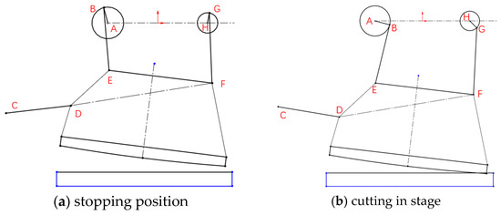
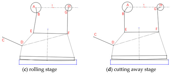
Figure 1.
Shearing process of Slitting Shear.
2.2. Vector Equation and Coordinate Transformation Theory of Kinematics of Mechanism
It is necessary to research the closed vector loop theory and coordinate transformation theory before establishing the kinematic mathematical model of the Slitting Shear cutting mechanism. The vector equation is established by drawing a vector diagram and connecting the member in the vector ring with a vector in a certain direction and forming a closed ring [11]. Figure 2 is a vector diagram of the linkage mechanism.
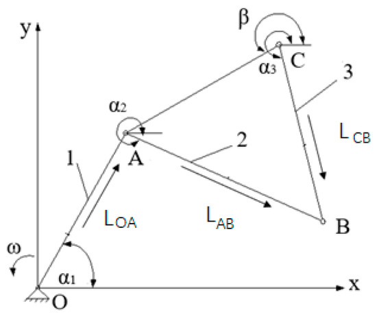
Figure 2.
Vector diagram of linkage mechanism.
Establish a vector equation for Figure 2.
Transform the above formula into the analytical formula.
The velocity and angular velocity equations at points A and B can be obtained by the first and second derivatives of Equation (2). Plane coordinate transformation is a process of transforming from one coordinate system to another one by establishing the corresponding relation between two coordinate systems. In Figure 3, point R in the double planar rectangular coordinate system is represented by [r]1 = [x1,y1]T and [r]2 = [x2,y2]T, respectively, with a common origin.
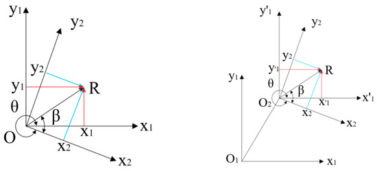
Figure 3.
Common origin and any plane rectangular coordinate system.
Easy to get , where the T12 matrix is the rotation transformation matrix of the coordinate systems from x2-O-y2 to x1-O-y1. On this basis, the parallel coordinate system x1-O1-y1 is introduced. Easy to Figure out from the vector equation, where is the coordinate transformation matrix of any plane coordinate system x2-O2-y2 to x1-O1-y1.
2.3. Kinematics Analysis of Slitting Shear Rolling Shearing
2.3.1. Displacement Equation of Slitting Shear Cutting Mechanism
The shear mechanism was simplified to get Figure 4, and an x-A-y fixed coordinate system was established. Where θ1 ∈ [0, 2π] is the positive angle between the crankshaft AB and the x-axis; θ2 ∈ [0, 2π] is the positive included angle between the crankshaft GH and x-axis; θ3 ∈ [0, π] is the positive included angle between the connecting rod BE, and the x-axis; θ4 ∈ [0, π] is the positive included angle of connecting rod HF and x-axis; θ5 ∈ [0, π] is the positive included angle of the upper tool table edge ED and x-axis; θ6 ∈ [−π/2, π/2] is the positive included angle between the rocker CD and the x-axis.
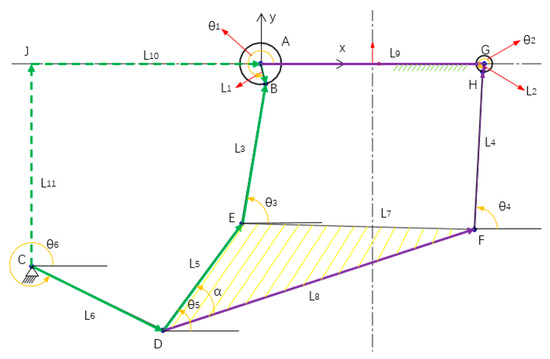
Figure 4.
Schematic diagram of Slitting Shear cutting mechanism.
Two vector loops, CDEBAJC and CDFHGAJC, were established based on the closed vector loop theory, and their vector equations were established, respectively. These equations were then transformed into analytical equations, which represent the displacement equations of the shearing mechanism.
The rod length and angle data of the cutting mechanism are presented in Table 1. The values of θ1 in different positions were obtained and calculated using Mathematica software. The curve depicting the angle variation is illustrated in Figure 5.

Table 1.
Rod length and angle parameters.
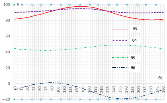
Figure 5.
Curve change of θ3, θ4, θ5, θ6.
Main motor and reducer parameters are known, crankshaft angular velocity ω1 = ω2 = 3.154 rad/s. Equation (3) takes the time derivative and obtains the angular velocity and angular acceleration curves through Mathematica software calculation, as shown in Figure 6.
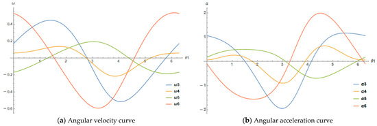
Figure 6.
Angular velocity and angular acceleration solve the curve.
2.3.2. Coordinate Equation and Trajectory Solution of Shear Mechanism Key Points
The trajectory analysis of the shear mechanism is primarily on the three hinge points of the top knife sledge and the dynamic lowest point of the top blade [12,13]. The coordinates of the three hinge points, E, F, and D, in the fixed coordinate system, can be obtained using vector equations.
After the Mathematica software solution, the coordinates of discrete points were plotted in the trajectory curve in Figure 7.
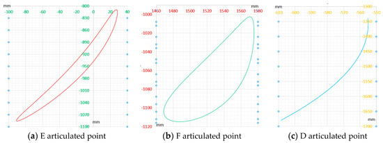
Figure 7.
Trajectory curve of the hinge point of the tool table.
To obtain the coordinate equation of the dynamic lowest point of the top blade, the dynamic coordinate systems x1-e-y1 and x2-e-y2 are introduced in Figure 4, as depicted in Figure 8. The x1-axis of the coordinate system x1-e-y1 coordinate system aligns with the EF of the top knife sledge, while the x2-axis of the x2-e-y2 coordinate system remains parallel to the x-axis of the fixed coordinate system. By solving the coordinates of the articulated point E in the fixed coordinate system x-A-y, the precise position of the top knife sledge in the fixed coordinate system can be determined, contingent upon the angle θ8 of the top knife sledge. The angle θ8, in turn, can be calculated by determining the coordinates of the hinged points E and F.
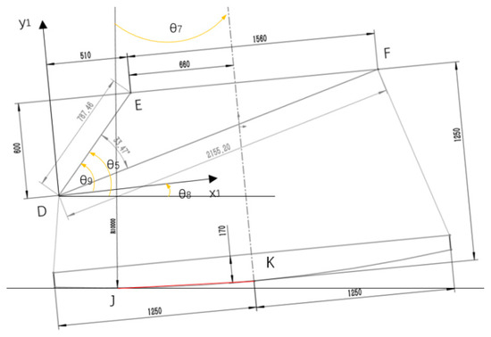
Figure 8.
Coordinates of any point on the top knife sledge.
The θ8 curve in Figure 9 can be obtained by substituting the angle data calculated by Mathematica software into Equation (5). After solving θ8, only the coordinates of the dynamic lowest point on the top knife sledge in the dynamic coordinate system need to be obtained. By performing the coordinate transformation, we can obtain the coordinates of the dynamic lowest point in the fixed coordinate system, allowing us to determine the trajectory curve and the overlap ratio data. We set the coordinates of any point S on top knife sledge as (xs1,ys1) in the dynamic coordinate system x1-E-y1, and the coordinates of any point S in the dynamic coordinate system x2-E-y2 after rotation coordinate transformation as (xs2,ys2). According to the rotation coordinate transformation theory, the following formula is obtained.
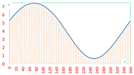
Figure 9.
Curve of the angle of the top knife sledge θ8.
Translate the coordinate (xs2,ys2) of any point S on the top knife sledge in the dynamic coordinate system y2-E-x2 into the coordinate (xs2,ys2) in the fixed coordinate system x-A-y after translation, can get , substituting Equations (4) and (6) into the can be obtained.
Equations (5) and (7) represent the coordinate formulas for any points on the top knife sledge. The radius of the top blade arc is R = 25,000 mm. Based on the geometric relationship in Figure 8, in the dynamic coordinate system x1-E-y1, the coordinates of the center of the top blade arc are (660, −23,750), and the coordinates of the endpoint M of the arc are (910, 1218.73). The coordinates of point M in x1-E-y1 were substituted into Equation (8) to obtain the coordinate Equation (7) of the midpoint of arc K in the fixed coordinate system. The trajectory curve of point K and the endpoint M of the circular arc was obtained by using Mathematica software, as shown in Figure 10.
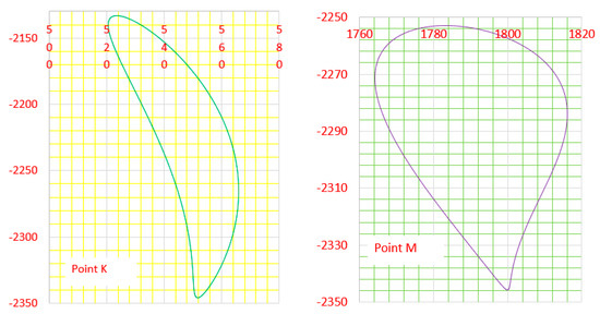
Figure 10.
Trajectory curve of the midpoint K and the endpoint M of the top blade arc.
According to the triangle similarity theorem, θ7 = θ8. In the shearing state, the line connecting the dynamic lowest point J of the top blade arc and the center of the arc is perpendicular to the x-axis of the fixed coordinate system x-A-y. The coordinates of the dynamic lowest point J can be easily obtained.
Since the dynamic lowest point J has a limit, geometrically, θ7 has a maximum value of θ7max = 2.866°. Therefore, the calculation should also restrict the corresponding angle of θ8 angles. By substituting Equation (8) into Equation (9), the coordinates of the dynamic lowest point on the top blade arc can be obtained.
Through Mathematica software, Equations (10) and (11) were solved to get the dynamic lowest point trajectory of the curve. The angle of crankshaft θ1 during the shear phase ranges from 232° to 352°, corresponding to the lower part of Figure 11a. The coordinates of the top surface of the bottom blade can be seen from the drawings as y = −2350 mm, and the overlap ratio curve can be obtained by comparison. The overlap ratio curve of the shearing stage is located at the right end of Figure 11b, as shown in Figure 11.

Figure 11.
Dynamic lowest point trajectories and overlap ratio curves.
2.4. Dynamic Simulation Verifying of the Cutting Mechanism of Slitting Shear
After the kinematics analysis of the cutting mechanism, necessary to simulate to verify the accuracy of the kinematics analysis results. In order to restore the contrast, the overlap ratio is also ignored.
2.4.1. Verify of Vector Equation and Dynamic Trajectory of Arc Lowest Point
To verify the accuracy of the calculation results of θ3, θ4, θ5 and θ6 by Mathematica software, Solidworks was used for verification. The sketching function of Solidworks was used to verify 6 groups of data, and θ1 was spaced 60° to obtain the mechanism diagrams of different angle positions. Through measurement, the data from various angles were collected in Table 2 and compared with the calculated data from Mathematica software. The maximum calculation error was 0.000281°, and the calculated results were consistent, thus proving the accuracy of the coordinate equation in the mathematical model.

Table 2.
Comparison of results of Solidworks and Mathematica.
In addition, Solidworks was utilized to validate the accuracy of the dynamic lowest point trajectory calculation for the arc of the top blade performed by Mathematica software. The sketch function was employed to verify 72 data sets, with θ1 incrementing at 5° intervals to generate mechanism diagrams at various angles. The coordinate data set was obtained by recording the horizontal and vertical coordinates of the lowest point on the arc of the upper cutting edge. It is worth noting that the dynamic lowest point J of the arc at a specific θ1 angle corresponds to the endpoint M of the arc. The verification method involved creating an auxiliary line perpendicular to the x-axis through the center of the arc. As the angle changed, the auxiliary line periodically perpendicular intersected or moved from the arc segment, explaining the boundary issue in Equations (10) and (11). The coordinate data was plotted to generate the trajectory curve shown in Figure 12, which was consistent with the results from Mathematica software. Additionally, the trajectory diagrams of hinged points E, F, D, and the endpoint M of the top blade arc were obtained, and the calculated results matched those obtained from Mathematica software. The same conclusion was reached using Solidworks Motion simulation [14]. The detailed process is not described here.
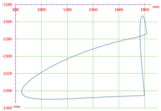
Figure 12.
Solidworks trajectory check of arc dynamic lowest point on the top blade.
2.4.2. Adams Virtual Prototype Simulation of Shearing Mechanism
Compared with Solidworks Motion, Adams is more professional in the kinematics simulation of mechanisms. In particular, its powerful Postprocessor module can output all kinds of data and curves from high-quality simulations [15,16]. The Solidworks model was imported into Adams for simulation analysis. The origin of coordinates was set at the hinge point between crankshaft I and the earth, as shown in Figure 13.
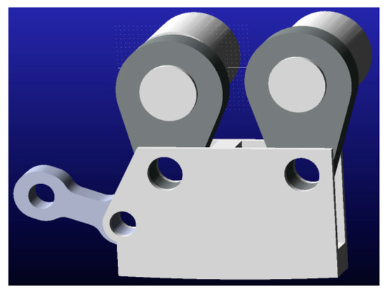
Figure 13.
Adams simulation model.
The crankshaft, guide rod, and earth were created rotation pairs, the upper cutter table was respectively created rotation pairs with connecting rod I, connecting rod II and guide rod, and the two crankshafts were created clockwise drive. After the simulation, the measurement function of the Postprocessor module was used to track and process the displacement of the x and y axes of each key point [17]. Then, the displacement was synthesized to obtain the motion trajectories of each key point in Figure 14, which was consistent with the calculation results of the analytical method mentioned above.
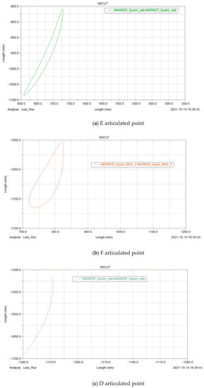
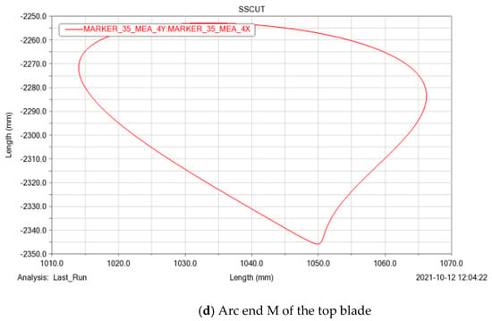
Figure 14.
Adams key point simulation trajectory diagram.
In order to accurately simulate the dynamic lowest point on the arc of the upper cutting edge, 51 points (J1, J2, J3…… J51), create 51 marker points in Adams with the coordinate data of each point. The earth was tracked by 51 markers using the measurement function. In the Postprocessor, time was taken as the abscissa, and the longitudinal displacement was taken as the ordinate. The longitudinal displacement curve of the marked points was drawn and placed in Figure 15. By fitting Figure 15 the longitudinal displacement curve of the dynamic lowest point can be obtained, as shown in Figure 16, which was consistent with the comparison with Figure 11. Thus, the analysis of the dynamic lowest point of the arc of the top blade in the mathematical model is correct.
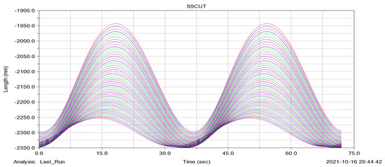
Figure 15.
Longitudinal displacement curve of each marked point.
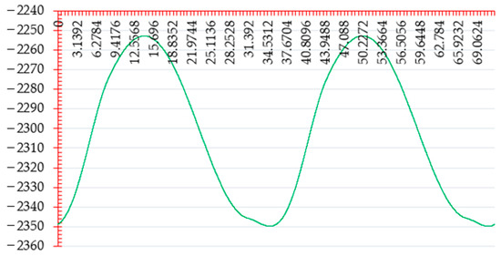
Figure 16.
Dynamic longitudinal displacement dynamic lowest point of top blade arc.
3. Research on the Relation between Blades Overlap Ratio and Steel Plate Thickness Based on Deform Finite Element
The cutting process of steel plates involves ductile fracture during metal shearing [18,19,20]. During shearing, plastic deformation occurs in the minimal area of the steel plate at the gap between the blades, ultimately resulting in fracture and separation of the steel plate [21]. To determine the overlap ratio of steel plates with different thicknesses, the Deform-3D finite element method is used to analyze the required cutting depth. Deform-3D is a rigid-plastic finite element method based on the revised Lagrange theorem. Fracture criteria are introduced to facilitate the finite element simulation of steel plate shearing [22,23]. Currently, Cockcroft & Latham’s fracture criterion has been found to be effective through extensive finite element simulations. When the deformation at a specific point in the material reaches this critical value, the fracture requirement is considered to be met. The mathematical expression of material critical value C is , Where σ* is the maximum tensile stress at the fracture of the material [24], Where σ1 is the maximum principal stress at fracture. The fracture criterion can be directly selected and set in Deform-3D. In this paper, the cell deletion method is used to simulate the fracture separation of materials in the program. In the simulation of section shear, when the stress and strain of the element reach the fracture criterion, the element is considered to have been cut. The unit is then removed from the model and doesn’t participate in further calculations. Import Solidworks model into Deform-3D. To reduce the computational workload, only the top blade of the knife mechanism is retained in modeling, while other parts are removed, but the positional relationship between parts should be maintained. Set the top and bottom blades and holding-down plates as rigid bodies.
The simulated Q345 steel plates were 25 mm and 30 mm thick. In the shear simulation, the deformation of the steel plate in contact with the blade was significant, leading to changes in the boundary condition and distortion or mesh overlap. To prevent the simulation from stopping, the mesh needs to be re-meshed. The element removal method is used to realize the separate elements. To avoid excessive deletion that may affect the simulation results, mesh subdivision should be performed by adding mesh panes to the steel plate at the shearing position. To prevent plate movement during shearing, a constraint of 0 velocities in the length direction was applied to the plate. Deform-3D also requires setting friction conditions for finite element analysis. A shear friction model of the plastic body was adopted, and the friction coefficient was set to 0.1. Additionally, contact was established between the top blade and steel plate, bottom blade and steel plate, and holding-down plate and steel plate. Figure 17a–f depict the analysis results of the shearing process of the steel plate. In Figure 17a, the top blade starts to press into the steel plate, resulting in high stress and strain at the contact point between the steel plate and the top blade. The steel plate is in the stage of elastic deformation. In Figure 17b, the stress and strain continue to increase, and the steel plate begins to crack. As shearing progresses, the stress and strain at the contact point between the top and bottom blades and the steel plate further increase, leading to the expansion of the crack. Figure 17c,d show the process of crack propagation until the plate breaks in Figure 17d.
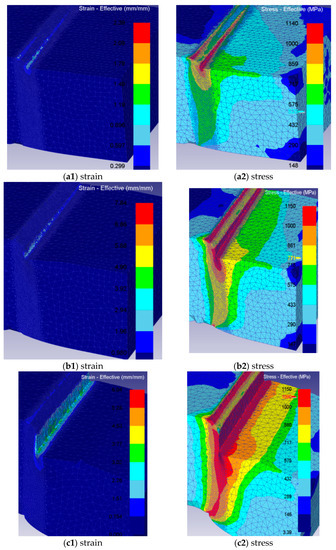
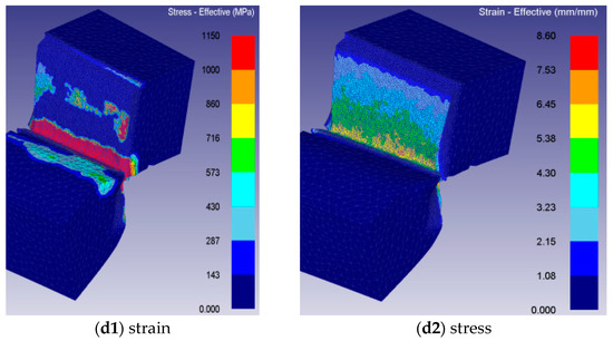
Figure 17.
Shearing process of steel plate.
The variation curve can be obtained by analyzing the shear depth and shear force results, as shown in Figure 18. As the thickness of the steel plate increases, the percentage of cutting depth corresponding to the maximum shear force decreases, indicating that the steel plate does not need to be completely cut in the shearing process to cause a fracture. The steel plate thickness, denoted as h, is equal to the sum of the overlap ratio, denoted as Gv, and the cutting depth, denoted as s, which can be expressed as h = Gv + s. The percentage of steel plate thickness and relative cutting depth in actual production is shown in Figure 19.
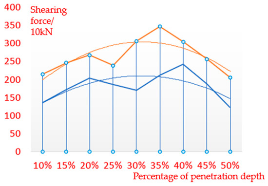
Figure 18.
Relationship between shear force and percentage of cut depth.
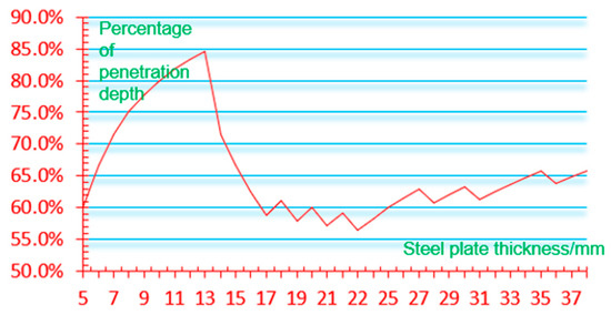
Figure 19.
Curve of the relationship between steel plate thickness and penetration depth in actual production.
It can be observed from Figure 19 that the distribution of the percentage of cutting depth is not uniform and appears relatively random. Selecting a cutting depth that is too large can significantly impact the shear quality of the steel plate. Due to certain limitations in adjusting the fit degree, it is necessary to ensure that the steel plate is fully divided. Based on the aforementioned research results, the corrected data for different fit overlap ratios can be obtained and are presented in Table 3. These data serve as the basis for practical application and as parameters for the optimization analysis in the paper.

Table 3.
Relationship between the thickness of the corrected steel plate, the overlap degree and the relative percentage.
4. Optimization Analysis of Shearing Mechanism’s Overlap Ratio Adjustment
4.1. Principle of Overlap Ratio Adjustment
See Figure 20 for the structure diagram of the single-side overlap ratio adjustment device of the Slitting Shear. The overlap ratio can be adjusted by changing the eccentric angle of the worm gear. The eccentric value of the worm gear is e = ±10 mm. In essence, the mechanism involves fine-tuning the length and angle of crankshaft I and II, along with the fixed rod length, within a certain range. This adjustment enables the repositioning of the ball bearing (lower end of the connecting rod), thereby changing the distance between the dynamic lowest point of the arc of the top blade and the bottom blade during shearing. After incorporating the overlap ratio adjustment mechanism, the modified mechanism diagram in Figure 21 is obtained from Figure 4. At this point, the length and angle of crankshaft I and II change. The hinge point B of crankshaft I becomes point P1, and the rod length changes from L1 to . The hinge point H of crankshaft II becomes P2 and the rod length changes from L2 to . The other lengths remain the same. The eccentric angle of the worm gear is measured counterclockwise from the crankshaft position, and its range is [0, π]. The hypothetical crankshaft rod lengths and remain unchanged throughout the shearing process after adjusting the overlap ratio.
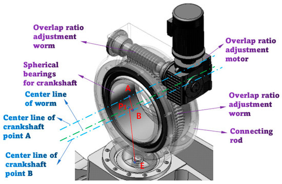
Figure 20.
One side overlap ratio adjustment model.
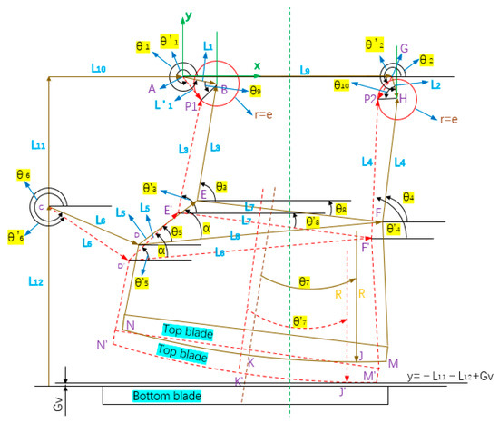
Figure 21.
Diagram of shear mechanism with overlap ratio adjustment.
4.2. Optimal Design Scheme of the Overlap Ratio Adjustment
The objective of the optimal design is to approximate the optimal solution of pure rolling cut when the target overlap ratio is reached. This problem falls under the category of optimization design of nonlinear equations in engineering problems [25]. The optimal design is depicted in Figure 22.
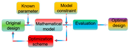
Figure 22.
Flow chart of optimization design.
In the process of solving optimization design, certain requirements need to be met, including the equations, design variables, objective functions, their allowable errors, and the constraints of the equations [26,27,28]. Given the target overlap ratio data, there exist infinite discretized data sets [29] for the hypothetical crankshaft rod length I and II that satisfy the desired outcome. However, since engineering problems require a certain level of precision, only one set of data can be optimal when a specific accuracy is specified. Therefore, the solving process involves determining the optimal solution among the infinite discrete data sets for the hypothetical crankshaft rod lengths I and II. The optimal solution for engineering mathematics problems typically involves dealing with nonlinear programming problems, and various methods can be employed, such as convex optimization algorithms, nonlinear least square methods [30], Lagrange multiplier theory, and constrained optimization methods [31,32]. In this paper, the constrained optimization method is utilized to optimize the solution. The process and scheme of optimization design are described in detail as follows.
The coordinate equation of the lowest point of the top blade arc and the objective function equation for the ordinate of the dynamic lowest point of the top blade arc are listed; Using and as design variables, the bar length range of crankshaft I and II is constrained, and the value of the objective function equation for the overlap ratio is obtained and compared with the vertical coordinate of the dynamic lowest point. The obtained value is treated as an error, and the acceptable error range is defined. The initial values of design variables are provided, and the optimization is performed once. The generated data equations are then solved and compared with the error range. If the error range is satisfied, the results are outputted. If not, the optimization scheme is employed to further optimize the solution, and the process is repeated. Once an iterative solution satisfies the error range, the rod length results for crankshaft I and crankshaft II are outputted. These results are then substituted into the eccentric angle equation for solving. Finally, the solution results from the previous step are substituted into the formula for solving the overlap ratio of crankshaft I and crankshaft II using the bisection method, and their respective overlap ratios and outputted as the final results.
4.3. Optimization Design of the Overlap Ratio
4.3.1. Equations and Design Variables
The rod length and angle in the vector Equation (3) of the shear mechanism are replaced with the data adjusted for the overlap ratio. Additionally, and are used as variables. Furthermore, the phase angle difference is no longer 25° due to the change in the crankshaft change.
Rod length and angle of crankshaft I and II in Equations (12) and (13) are replaced as variables to get Equation (14).
The dynamic lowest point of the top blade exists only on the arc, which is easy to know from the geometric relationship of the top blade.
4.3.2. Objective Function, Its Allowable Errors and Model Constraints
When considering the overlap ratio between the dynamic lowest point of the top blade arc and the bottom blade, it can be divided into positive and negative values. A positive value indicates that there is no overlap between the top and bottom blades, while a negative value indicates the presence of overlap. The ordinate function for the position of the target overlap degree is , where GV is evaluated in Table 3. The error between the vertical coordinate of the actual arc dynamic lowest point of the top blade arc and the target overlap ratio line is denoted as ΔV. When ΔV is positive, it means that the dynamic lowest point of the top blade is above the straight line y. When it is negative, there is:
When the error ratio ΔV to overlap ratio GV is limited and preliminarily set at ±5%, the trajectory of the dynamic lowest point of the top blade arc approaches a horizontal straight line and closely aligns with the target overlap ratio line. This ensures that the requirement for an approximate pure rolling cut is met. Then , since the eccentric e of the worm gear of both crankshafts is 10 mm, the range of sum that can be obtained from the triangle theorem is .
4.3.3. Optimization Method
The optimal design method employed in this paper is the constrained nonlinear optimization algorithm, which consists of the direct search method and gradient-based algorithms. Direct search methods, such as Nelder–Mead [33], genetic algorithms, and differential evolution, do not rely on derivative information, resulting in slower convergence but more relaxed constraints on functions and constraints. Gradient-based algorithms, on the other hand, utilize first or second derivatives [34], such as sequential quadratic programming (SQP), Lagrange methods, and nonlinear interior point methods [35]. The gradient-based algorithm can be further categorized into the gradient descent method and the conjugate gradient method [36]. The former exhibits significantly slower convergence near the optimal solution and requires multiple iterations. The conjugate gradient [37,38] method, on the other hand, utilizes only one level of information and achieves a computational speed between the steepest descent method and Newton’s method. It overcomes the drawbacks of slow convergence and avoids the need for storage and computation of the Hesse matrix, making it one of the most effective methods for solving large nonlinear equations [39,40,41]. In general, the algorithm builds only a local model of the problem. In the Mathematica language, the global optimization algorithm usually tries to find the optimal global solution by allowing both decreasing and increasing the optimal value function of the objective function. The global optimization problem can be solved precisely or numerically by using the NMinmize function. In this paper, the NMinmize function algorithm used in the Mathematica language is shown in the following formula.
4.3.4. Optimized Design Result
After GV is given and a pair of sum values are calculated by the Mathematica optimization, the angles of two eccentricities can be calculated by the cosine theorem. Part of the optimization results are shown in Table 4.

Table 4.
Mathematica optimization design results.
5. Conclusions
Mathematical modeling is undoubtedly an effective approach to approximate the desired trajectory when studying planar multi-linkage with numerous degrees of freedom. Compared to analytical methods, optimization methods offer higher accuracy in solving nonlinear equations and allow for extensive search and iteration until a practical engineering solution is achieved. The investigation of the overlap ratio in Slitting Shear fundamentally involves the study of the kinematic mathematics of a two-DOF mechanism. In this paper, a one-DOF motion mathematical model is initially established without considering the overlap ratio, which is then validated through simulation. Building upon this mathematical model, the overlap ratio is introduced, and a three-DOF mathematical model of the shearing mechanism is developed. Finally, utilizing the conjugate gradient method and the global optimal NMinimize function, the overlap ratio setting is optimized and solved. By satisfying the overlap ratio requirement, the solution for the two-DOF mechanism approximating pure rolling cut is obtained. The key contributions of this paper are outlined as follows:
- (1)
- The mathematical modeling of the section shearing mechanism was performed through vector equations and coordinate transformations. Kinematics equations, angular velocity equations, angular acceleration equations, and coordinate equations for any point on the top knife sledge were derived. Mathematica software was utilized for equation programming to obtain angles, angular velocities, angular accelerations, and trajectory curves;
- (2)
- Solidworks and Adams software were employed to simulate the shear mechanism and validate the reliability of the mathematical model;
- (3)
- The shear fracture mechanism of the steel plate was introduced, and based on Cockcroft & Latham’s fracture criterion, finite element analysis of the steel plate shearing process was conducted using Deform-3D software. The relationship between the cutting depth of the steel plate and maximum shear force was studied, recommended cutting depths for steel plates with different thicknesses were derived, and guiding data for the contact degree were obtained;
- (4)
- In the process of pure rolling cut, the dynamic trajectory of the lowest point of the top blade in the rolling shear approximates a horizontal straight line. Unlike other rolling shears with fixed trajectories, the Slitting Shear requires trajectory adjustment based on the steel plate thickness while considering the requirements for pure rolling cut and meeting the target overlap ratio. In this paper, an optimization algorithm based on the conjugate gradient method is employed to achieve these two objectives and obtain the recommended value for overlap ratio adjustment.
The current finite element analysis calculations in the shearing process are extensive. Due to resource limitations, the number of analyzed samples in this paper is limited, and actual data on overlap ratios for steel plates of different thicknesses are lacking. Additionally, the analysis process does not consider different steel types, hence requiring more analysis samples to obtain more accurate data. This represents a direction for further research.
Author Contributions
W.F. and Y.L.: Conceptualization. Y.L.: Methodology, project administration, funding acquisition. W.F.: software, validation, formal analysis, data curation, processing, writing—original draft preparation and writing—review and editing. J.L. and Z.D.: resources, writing review and editing. M.L. and W.S.: investigation, supervision. All authors have read and agreed to the published version of the manuscript.
Funding
This research received no external funding.
Data Availability Statement
All data included in this study are available upon request by contact with the corresponding author.
Conflicts of Interest
The authors declare that there is no conflict of interests regarding the publication of this article.
References
- Kim, J.; Yoon, J. Development of a new Slitting Shear for cutting thick plates. J. Mech. Sci. Technol. 2018, 32, 2789–2796. [Google Scholar]
- Wang, Z.; Han, J.; Yu, X. Analysis of the shear process and design of the blade of Slitting Shear. J. Mater. Process. Technol. 2009, 209, 3489–3494. [Google Scholar]
- Wang, H.; Huang, W.; Liu, Y. Design optimization of seven-bar mechanism based on differential evolution algorithm. J. Mech. Sci. Technol. 2021, 35, 2275–2286. [Google Scholar]
- Li, X.; Li, X.; Li, B.; Li, Y.; Li, S. A study on optimization of the cutting edge curve of rolling shear with improved PSO algorithm. J. Intell. Manuf. 2018, 29, 1273–1285. [Google Scholar]
- Liu, J.; Yan, J.; Yang, S.X. Chaotic optimization of a four-bar linkage mechanism for optimal energy transfer. Mech. Mach. Theory 2016, 103, 1–14. [Google Scholar]
- Zhang, Y.; Wang, X.; Gao, Y. Optimization of chaotic motion of linkage mechanism based on genetic algorithm. J. Mech. Sci. Technol. 2016, 30, 2559–2564. [Google Scholar]
- Gao, J.; Li, M.; Allison, G.; Cui, L. Optimal dimensional synthesis of a symmetrical five-bar planar upper-extremity neuromotor device. Chin. J. Mech. Eng. 2015, 28, 684–690. [Google Scholar] [CrossRef]
- Konzel, E.C.; Huang, Q.; Lin, F. Geometric constraint methods in trajectory synthesis for mechanisms. Mech. Mach. Theory 1993, 28, 499–513. [Google Scholar] [CrossRef]
- Chen, J.; Zhang, C.; Chen, G. Design and analysis of circular arc top blade slitting mechanism for longitudinal shear. J. Phys. Conf. Ser. 2019, 1261, 012018. [Google Scholar] [CrossRef]
- Zhang, C.; Chen, J.; Chen, G. Design of slitting mechanism with circular arc top blade based on finite element analysis. J. Phys. Conf. Ser. 2018, 1071, 012034. [Google Scholar] [CrossRef]
- Bandyopadhyay, A. Vector Ring: A Better Way to Understand Vector Addition. Resonance 2018, 23, 383–392. [Google Scholar]
- Zhang, Y.; Zhang, W.; Wang, J.; Dong, C. Trajectory Analysis of Shearing Mechanism Based on Three Hinged Points and Dynamic Lowest Point. J. Phys. Conf. Ser. 2019, 1334, 012071. [Google Scholar] [CrossRef]
- Zhang, J.; Wang, Z.; Zhang, Y. Design and analysis of a rolling shear cutter with dynamic optimization of the upper blade. Int. J. Adv. Manuf. Technol. 2014, 75, 1903–1913. [Google Scholar]
- Kurowski, P.M. Engineering Analysis with Solidworks Simulation; SDC Publications: Mission, KS, USA, 2015. [Google Scholar]
- Chen, Z.; Jiang, W.; Li, X. Research on the Application of ADMAS Software in Structural Dynamic Analysis. J. Phys. Conf. Ser. 2018, 1091, 012021. [Google Scholar] [CrossRef]
- Zhu, Y.; Xiong, W.; Shen, X. Research on the Post-Processing Module of ADMAS Software in Mechanical Engineering Design. J. Phys. Conf. Ser. 2021, 1874, 012031. [Google Scholar]
- Li, Y.; Cai, L.; Xu, L. Dynamic performance analysis of a planar six-bar linkage based on multi-body dynamics simulation. Int. J. Adv. Manuf. Technol. 2020, 107, 3153–3163. [Google Scholar] [CrossRef]
- Lou, Y.; Yoon, J.W.; Huh, H. Modeling of shear ductile fracture considering a changeable cut-off value for stress triaxiality. Int. J. Plast. 2014, 54, 56–80. [Google Scholar] [CrossRef]
- Basak, S.; Kim, C.; Jeong, W.; Jung, Y.I.; Lee, M.G. Numerical prediction of sheared edge profiles in sheet metal trimming using ductile fracture modeling. Int. J. Mech. Sci. 2022, 219, 107109. [Google Scholar] [CrossRef]
- Lou, Y.; Chen, L.; Clausmeyer, T.; Tekkaya, A.E.; Yoon, J.W. Modeling of ductile fracture from shear to balanced biaxial tension for sheet metals. Int. J. Solids Struct. 2017, 112, 169–184. [Google Scholar] [CrossRef]
- Allwood, J.M.; Lam, A.C. An experimental and numerical investigation of shear banding in mild steel. Int. J. Mech. Sci. 2000, 42, 1469–1490. [Google Scholar]
- Ko, D.C.; Kim, B.M.; Choi, J.C. Finite-element simulation of the shear process using the element-kill method. J. Mater. Process. Technol. 1997, 72, 129–140. [Google Scholar] [CrossRef]
- El-Zafrany, A.; Bai, Y. Numerical simulation of sheet metal shearing using a non-local fracture criterion. Int. J. Mech. Sci. 2016, 116, 3–14. [Google Scholar]
- M’Saoubi, M.; Miguélez, H. Prediction of the fracture behavior in sheet metal forming using Cockcroft-Latham criterion. J. Mater. Process. Technol. 2001, 116, 246–252. [Google Scholar]
- Wang, Y.; Zhang, L.; Zhang, W. Optimization Design of Nonlinear Equations in Engineering Problems Based on Improved Genetic Algorithm. Math. Probl. Eng. 2018, 2018, 1745083. [Google Scholar]
- Kuhn, H.W.; Tucker, A.W. Nonlinear programming. In Traces and Emergence of Nonlinear Programming; Springer: Basel, Switzerland, 2013; pp. 247–258. [Google Scholar]
- Malyuta, D.; Reynolds, T.P.; Szmuk, M.; Lew, T.; Bonalli, R.; Pavone, M.; Acikmese, B. Convex optimization for trajectory generation. arXiv 2021, arXiv:2106.09125. [Google Scholar]
- Maghawry, A.; Hodhod, R.; Omar, Y.; Kholief, M. An approach for optimizing multi-objective problems using hybrid genetic algorithms. Soft Comput. 2021, 25, 389–405. [Google Scholar] [CrossRef]
- Shaari, M.S.; Rahman, M.M.; Noor, M.M.; Kadirgama, K.; Amirruddin, A.K. Design of connecting rod of internal combustion engine: A topology optimization approach. In Proceedings of the National Conference in Mechanical Engineering Research and Postgraduate Studies (2nd NCMER 2010), Kuantan, Malaysia, 3–4 December 2010; Volume 155, p. 166. [Google Scholar]
- Sahu, D.R.; Pitea, A.; Verma, M. A new iteration technique for nonlinear operators as concerns convex programming and feasibility problems. Numer. Algorithms 2020, 83, 421–449. [Google Scholar] [CrossRef]
- Nocedal, J.; Wright, S.J. Numerical Optimization, 2nd ed.; Springer Science & Business Media: Berlin/Heidelberg, Germany, 2006. [Google Scholar]
- Jahn, J. Introduction to the Theory of Nonlinear Optimization; Springer: Cham, Switzerland, 2020. [Google Scholar]
- Kolda, T.G.; Lewis, R.M.; Torczon, V. Optimization by direct search: New perspectives on some classical and modern methods. SIAM Rev. 2013, 55, 373–407. [Google Scholar] [CrossRef]
- Ruder, S. An overview of gradient descent optimization algorithms. arXiv 2016, arXiv:1609.04747. [Google Scholar]
- Bottou, L. Large-scale machine learning with stochastic gradient descent. In Proceedings of the COMPSTAT’2010: 19th International Conference on Computational Statistics, Paris, France, 22–27 August 2010; pp. 177–186. [Google Scholar]
- Bubeck, S. Convex optimization: Algorithms and complexity. Found. Trends® Mach. Learn. 2015, 8, 231–357. [Google Scholar] [CrossRef]
- Saad, Y. Iterative Methods for Sparse Linear Systems, 2nd ed.; Society for Industrial and Applied Mathematics: Philadelphia, PA, USA, 2003. [Google Scholar]
- Golub, G.H.; Van Loan, C.F. Matrix Computations, 4th ed.; Johns Hopkins University Press: Baltimore, MD, USA, 2012. [Google Scholar]
- Wang, G.; Sun, W. A new trust-region method for nonlinear equations without calculation of the Hessian matrix. J. Comput. Appl. Math. 2016, 302, 306–320. [Google Scholar]
- Zhang, J.; Wang, Y. A new trust region method for nonlinear equations. Math. Methods Oper. Res. 2003, 58, 283–298. [Google Scholar] [CrossRef]
- Li, D.; Li, D.; Sun, W. A new trust region method for large-scale nonlinear equations with application to the simulation of lithography process. Appl. Numer. Math. 2017, 115, 19–31. [Google Scholar]
Disclaimer/Publisher’s Note: The statements, opinions and data contained in all publications are solely those of the individual author(s) and contributor(s) and not of MDPI and/or the editor(s). MDPI and/or the editor(s) disclaim responsibility for any injury to people or property resulting from any ideas, methods, instructions or products referred to in the content. |
© 2023 by the authors. Licensee MDPI, Basel, Switzerland. This article is an open access article distributed under the terms and conditions of the Creative Commons Attribution (CC BY) license (https://creativecommons.org/licenses/by/4.0/).