Abstract
The proliferation of Industry 4.0 (I4.0) technologies has created a new manufacturing landscape for manufacturing, requiring that companies follow I4.0 trends to stay competitive. However, in this novel digital automated environment, these companies must also ensure that lean manufacturing principles are upheld. This study proposes a data-driven framework for analysing raw data across machines in manufacturing systems that can provide a comprehensive understanding of idle time and facilitate adjustments to reduce defect rates. This framework offers an alternative approach to improving manufacturing processes that involves utilising the power of I4.0 technologies in conjunction with lean manufacturing principles. This study’s examination of unprocessed data also provides guidance on improving legislation. The findings of this study provide direction for future research in the field of manufacturing and offer useful advice to businesses wishing to integrate I4.0 technologies into their operations.
1. Introduction
The fourth industrial revolution, Industry 4.0 (I4.0), is positioned to enhance automation, productivity, quality, reliability, efficiency and cost-effectiveness in different industrial sectors, including manufacturing [1]. The development towards I4.0 has significantly influenced manufacturing industry trends [2]. I4.0 implementations produce materials and goods using highly automated and mechanised processes performed using a combination of smart factories, cyber-physical systems (CPSs), self-organisation and novel distribution and procurement systems to adapt to human needs [3]. One of the central I4.0 concepts, CPS, is responsible for the ‘3Cs’ of computing, communication and control, which deliver benefits, including real-time sensing, information feedback and dynamic control [4].
I4.0 also significantly contributes to companies changing their manufacturing practices, especially the constant need to adapt to customer needs [5]. Machines can be retooled to make them self-learning and self-aware, improving their overall performance and simplifying their maintenance in line with the context [6]. To closely integrate the Internet of Things (IoT) business model, research has pursued the ‘future of intelligent manufacturing’ [7] (p. 308), recognising that the ‘IoT was born to break the darkness constraint and create information without observation from humans in various situations previously unseen’ [8] (p. 5). In contrast with traditional data acquisition, which involves gathering information from a small number of sources in a controlled environment, the IoT data acquisition entails gathering a large amount of information from numerous sources, frequently, in real-time, using a network of connected sensors, devices and systems. Some sensors detect and measure the environment in which they are deployed and translate the processing input into electrical signals. For example, MEMS sensors, Arduino and Raspberry Pi are open-source components used for sensing, processing and controlling data [9]. To manage the substantial amounts of data produced by these devices, sophisticated technologies and procedures are needed [10]. To facilitate IoT data acquisition, platforms have been designed to build and prototype IoT applications, with Intel Edison commonly used to collect, process and transmit data from the environment, which is critical to the data ingestion process [11].
Building on the advantages of connectivity provided by the IoT, access to reliable data and the creation of cyber-physical frameworks, I4.0 has recently focused on online technology at a completely new level. Thus, I4.0 proposes a more comprehensive, integrated and all-encompassing development paradigm [12]. The automation and data exchange in manufacturing technologies have merged with the industrial IoT to create manufacturing systems that are not only interconnected, but also capable of communicating, analysing and using information to drive further intelligent actions in the physical world. Via the self-diagnosis of IoT-enabled equipment, abnormal circumstances can be identified. In other words, potential failures and defects can be anticipated rationally and a set of corresponding optimisation solutions can be designed proactively [13]. However, the technology level of many manufacturers remains at the Industry 3.0 level due to their lack of capital, which is necessary to purchase new machines or systems and obtain the related knowledge.
Many manufacturers are actively participating in upgrading their factories to ‘smart factories’ to adhere to the standards expected under the I4.0 paradigm. By internally sharing real-time information with different departments in factories, various forms of manufacturing intelligence can be obtained [14]. For example, using digital twins, companies can monitor and visualise manufacturing processes in virtual replicas of actual systems [14], continuously track the condition and state of different systems and predict the system’s performance in terms of finding data, allowing for decisions to be determined. Smart manufacturing tools and a transparent system allow for easy adaptation to schedule changeovers and update plant layouts without large-scale interventions, increasing flexibility [14]. Meanwhile, cloud-based architectures of smart factories offer numerous advantages, including flexibility, scalability and cost-efficiency. However, to ensure the success of cloud-based solutions, it is critical to resolve security, privacy and latency challenges. To increase data security and privacy, it is important to use encrypted data, dispersed data storage and secure communication protocols, with edge computing and fog computing reducing latency difficulties by processing data closer to the source [15]. Nonetheless, as mentioned, for many manufacturers (especially those in China), upgrading factories to I4.0 standards is complicated by the vast amounts of capital required to purchase the necessary machines and systems. Moreover, expert knowledge is required to perform the upgrade. It is difficult to facilitate machines sharing data and determining adjustments without connecting to a CPS, and it is difficult for firms to adjust machines’ data settings without the support of data analysis. This is important because it represents the most ideal and cost-effective method of adhering to I4.0 practices: manufacturers collect data and determine the major parameters that affect the defect rate to determine informed decisions that allow them to control and reduce these defect rates.
The industrial IoT is critical to the collection of information and the automation of physical processes, representing the foundation of a fully digitalised facility by combining the cloud, analytics and artificial intelligence (AI) to create new operational models based on automation and augmented human activities that rely on predictive analyses for operations and maintenance, production and inventory monitoring and security improvements. In addition, AI and machine learning algorithms are powerful tools that address IoT challenges (including high-noise environments, versatile operating conditions and cross-domain machining) by developing models that can identify and adapt to different scenarios [16]. However, some of the current failure prevention processes are reactive to defects/faults, potentially resulting in wasted production and additional effort due to the need for remanufacturing. Thus, to correspond with the goals of smart manufacturing, contemporary research projects seek to modify such processes, such that they become proactive and autonomous [17].
To understand the information that can be gained from the raw data concerning the idle time of the manufacturing process of injection moulding, this study aims to achieve four objectives:
- To understand and analyse the data on injection moulding levels to track idle time levels;
- To determine abnormal idle time;
- To classify the different levels of abnormal idle time of injection moulding machines;
- To indicate the total idle time achieved.
2. A Data-Driven Approach
A data-driven approach involves determining decisions based on the analysis and interpretation of data [18]. This approach ensures that solutions and plans are supported by information and entails collecting and analysing data to explore solutions and provide insights. I4.0 is a data-driven paradigm because it utilises data to create more value. Many I4.0 technologies relate, in some way, to data [19]. Current advances in data processing algorithms coupled with lower computing costs allow for companies to analyse and improve their systems using automated means. The primary requirement for using these algorithms effectively is having access to large quantities of accurate data [14]. Many companies face the challenge of using existing databases for the optimisation of manufacturing processes. Previous studies have presented different methodologies for this activity, particularly focusing on methods of using and extending existing databases.
The most important component of a data-driven approach is data collection. A general method for collecting data from manufacturing systems is needed. Ideally, this data collection system should satisfy the following requirements: extendibility, being vendor-agnostic, nonintrusive, plug-and-play, usability and security. Usability and security are arguably the most important of these requirements. In terms of usability, the generated data must be reliable for and suited to the intended purposes, because the type of analysis changes based on the demands of various stakeholders. Hence, it should be possible, via additional analyses, to reuse the data collected to meet new demands. In terms of security, there must be a provision to enforce security in terms of the accessibility, storage and retrieval of data. This study’s goal is to provide tools that enable the collection and analysis of data from existing manufacturing stations. These tools could not only help manufacturers understand and improve existing systems, but also support them through I4.0 technologies [14].
2.1. Transformation
Data are the main factor in a data-driven approach. However, because raw data do not usefully provide intelligence, these data must be ‘transformed’ into something useful, which is usually achieved in several stages.
2.2. A Data-Driven Framework
This study adopted a two-stage data-driven framework to complete the classification [20] (Figure 1). The first stage, the design and training stage, involved cleaning all the input data using a MySQL query through DataGrip and preprocessing to ensure a better result, after which the cleaned data were analysed statistically.
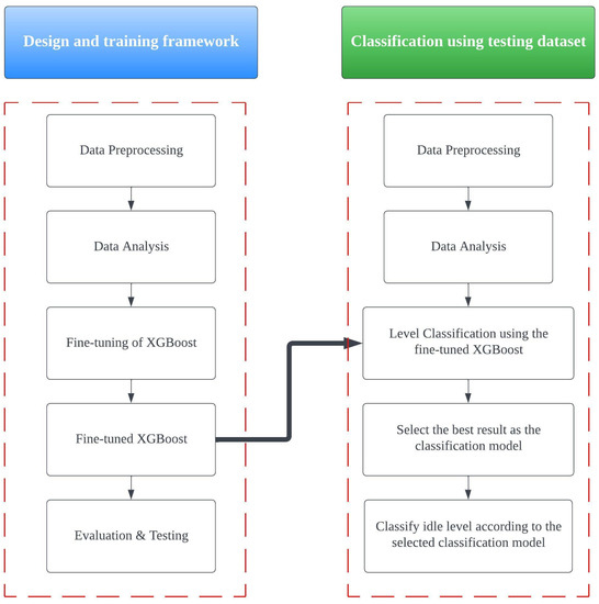
Figure 1.
The two-stage data-driven framework.
As an initial attempt, 30 machines were investigated. Two ratios, namely, the efficiency score and problem ratio, were calculated to determine each machine’s performance efficiency. A machine’s efficiency score e was calculated by dividing the machine running time R by machine idle time T, as represented by Equation (1). In this analysis, the higher the efficiency score, the more efficient the machine. The problem ratio p was calculated as the ratio of the machine adjusting time A to machine pause time P, as represented by Equation (2).
Using these efficiency scores and problem ratios, an efficiency and problem ratio matrix was created to classify all the machines. High-efficiency scores and high problem ratios resulted in better production performance. Machines with efficiency scores higher than the average score of all machines were considered to demonstrate high levels of efficiency. Similarly, machines with higher problem ratios than the average ratios of all machines were considered to have low potential for problems. The results enabled machine-handling priority to be determined for better time and resource management.
Once all the data were statistically analysed, a trend analysis was conducted to investigate the relationship between the machine idle time and time. Each machine’s trend was classified as upward, downward or almost stationary, classifications that were then used to prioritise machine handling. Meanwhile, graphs showing the total monthly idle time for the 30 machines combined were generated. Based on the trend analysis result, basic idle time statistics—including the mean, median, first quartile (Q1) and third quartile (Q3)—were calculated to determine (1) the indicator of abnormal idle time and (2) the concentration of abnormal idle time in a given period. Data points exceeding the indicator of abnormal idle time (i.e., mean idle time) were considered abnormal idle time. Compared to the median, Q1 and Q3, the mean was generally the largest. Therefore, the dataset may have been rightly skewed. Using the mean as the indicator reduced the risk of overestimation. Concerning the concentration of abnormal idle time in a period, seven different period lengths were considered: three days, four days, five days, six days, seven days, ten days and fourteen days. The prediction accuracy of different period lengths was compared, and the length with the best prediction accuracy (exceeding 90%) was selected as the most suitable model.
To gain a deeper understanding of abnormal idle time levels, XGBoost, a popular algorithm for supervised machine learning that uses decision trees and gradient boosting to improve the predictive accuracy [21], was first applied with default settings for the classification. X1 to X5 were the model’s input parameters, with X1 referring to the total number of entries, X2 denoting the running status, X3 the adjusting status, X4 the pausing status and X5 the offline status. Y referred to the level of abnormal idle time occurrences (output). Three levels of abnormal idle time occurrences were classified: low (denoted by 0), medium (denoted by 1) and high (denoted by 2). Eighty percent of the data was used as the training dataset, and the remaining twenty percent was used as the testing dataset. In XGBoost, many parameters could be adjusted. However, to produce better results, only certain selected parameters were fine-tuned in our study: eta (default = 0.3); gamma (default = 0); max_depth (default = 6); min_child_weight (default = 1); subsample (default = 1). The parameters were updated during the optimisation process, with the fine-tuned XGBoost evaluated and tested following a white box approach [22], involving understanding and interpreting the internal logic of the software to, thus, provide insights into how it behaves and how it can be improved [23]. After optimising XGBoost, it was applied for the level classification, the phase in the classification stage (see Figure 1) during which data were preprocessed and analysed. The aspects with the highest accuracy levels were selected as the target models due to the speed and accuracy delivered [24]. Then, all the remaining data were classified using the selected classification model. For the update policy of the indicator of abnormal idle time, the median absolute deviation (MAD) was used to determine the moving average in a day. This served as a useful indicator for observing the abnormal idle time because the MAD represented a measure of the average distance between each data point and the mean.
After calculating and analysing idle time at the machine level, idle time during in-house transit processes was analysed, with the in-house track and trace used to collect data for the subsequent calculation of statistical indexes and ratios for the in-house transits.
Using a workflow resembling the design and training stage—including data cleansing and preprocessing—enabled a data analysis identifying the overall functioning of the transportation time of different in-house transit processes. The basic statistical indexes and ratios, before and after the removal of outliers according to the upper control limit of each in-house transit type, were calculated to monitor and improve the quality of in-house transit processes for manufacturers. These statistical indexes were also used to determine the usual operation time, the upper limits of the transportation time, the lower limits of the transportation time and the stability. The statistical indexes of each in-house transit, before and after the removal of outliers, were then compared to highlight the significance of in-house transit and determine the significant changes across different in-house transit types and significant months. The first indicator was the mean of the overall data, which could be used to obtain preliminary observations and compare the general operation of the four types of in-house transits. The second indicator was the mean of the corresponding type of in-house transit.
Machines were labelled from five perspectives: average idle time levels (‘avg lv.’), total number of records (‘record lv.’), concentration of abnormal idle time level (‘den lv.’), ratio of adjusting (‘adjusting’) and ratio of pause (‘pause’). This labelling was based on Q1 and Q3, which were used for classification using the XGBoost package in Python through PyCharm and to plot the confusion matrix to determine the number of occurrences of abnormal idle time (i.e., the concentration) and demonstrate the accuracy of the classification. The label was then visualised using a simple table.
The update policy component used the variance of the moving average to identify the balance of the workload and sensitivity to suggest how often the indicator of abnormal idle time should be updated. For the track-and-trace measurement models, the lower and upper quartiles were calculated to identify the indicator for each type of in-house transit, with two different indicators employed.
3. Case Study of a Manufacturing Site
L.A. International Holdings (alias, affiliated as L.A.) was established in Hong Kong in 1980. L.A. is renowned for providing a variety of one-stop services to local and global communities. Due to global trends centring on implementing I4.0 technologies in factories, L.A. aimed to establish a smarter and more digital management system, allowing for the company to determine problems and react immediately in a cost-effective manner. L.A. achieved the 1i level of I4.0 (enhanced data availability) and was on track to achieve the 2i level (enhanced interpretability). However, the manufacturing site had some problems, such as the long idle time of the injection moulding machines (due to long waiting times or long transportation times). L.A. could analyse data to reduce this idle time and reduce the idle time of in-house transits to ensure higher levels of productivity.
3.1. Injection Moulding Machines
3.1.1. Data Preprocessing
L.A. aimed to reduce the idle time of their injection moulding machines and increase the visibility and traceability of the cycle times and process parameters. The original data was tabulated in a table for the injection moulding machines featured six columns: RecordID, MachineID, ProdID, Parameter, CreationTime and Status. This large table included all machines numbered 1 to 30, with creation times listed in ascending order. Due to this study only investigating these 30 machines, MachineIDs outside the 1–30 range were eliminated from the table. This reduced the original 317,203 records to 314,012 records. Subsequently, the large table was divided into 30 tables according to the MachineID, with the time differences for each machine then calculated.
3.1.2. Data Analysis
The efficiency scores of the machines appear in Figure 2 in descending order. In this analysis, the higher the efficiency score, the more efficient the machine. For instance, the machine with MachineID 13 was the most efficient machine, recording an efficiency score of 2.249, and with MachineID 24 being the least efficient machine, recording an efficiency score of only 0.697.
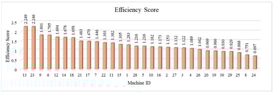
Figure 2.
The efficiency scores of machines.
Figure 3 shows the problem ratios of the machines in descending order. Machine with MachineID 9 recorded the largest problem ratio (0.272), suggesting that a machine error might have led to a high adjusting time. Meanwhile, machine with MachineID 21 recorded the smallest problem ratio (0.074), signalling a high pause time. This indicated the need for more comprehensive and efficient production planning.
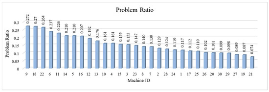
Figure 3.
The problem ratios of machines.
Outliers that might have affected the accuracy of the results were removed from the dataset to determine the machines’ actual performances (idle time) and produce useful information for processing, with 4304 fewer data points obtained after removing outliers (an average of approximately 2.73% for each machine). Figure 4 shows the efficiency and problem ratio matrix created for the classification of machines before and after the removal of outliers. Machines with the same position in the matrix before and after the removal of outliers were underlined for improved accessibility. Figure 4 reveals that the position of machines in the efficiency and problem ratio matrix varied significantly before and after removing the outliers.
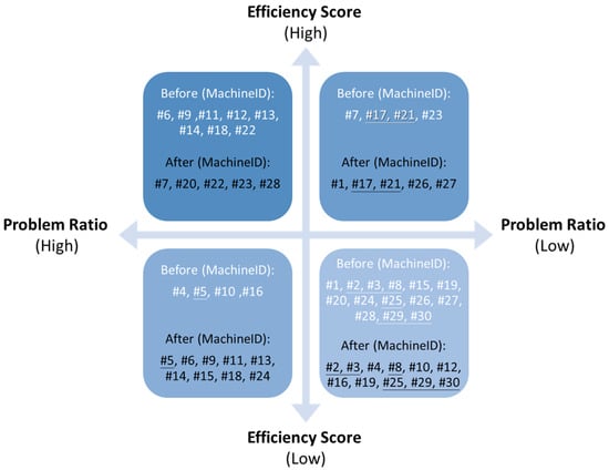
Figure 4.
Efficiency and problem ratio matrix before and after the removal of outliers.
3.1.3. Trend Analysis
Analysing the relationship between the machine idle time and time revealed that almost all of the idle time of the machines was either almost stationary or increased over time before removing outliers, while almost all machine idle time increased over time without any decreasing trends after removing outliers (Figure 5). Figure 6 and Figure 7 show the trend analysis of the total idle time of the 30 machines over time before and after the removal of outliers. The overall trend of all machine idle times slightly increased over time before the removal of outliers and became strictly increasing after the removal of outliers.
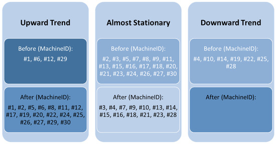
Figure 5.
The relationship between idle time and time before and after the removal of outliers.
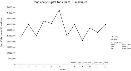
Figure 6.
The relationship between idle time and time before the removal of outliers.
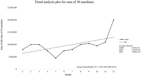
Figure 7.
The relationship between idle time and time after the removal of outliers.
3.1.4. Model Selection
Due to the significant increasing idle time over time both before and after removing outlying data points, abnormal idle time needed to be investigated in more depth. The mean idle time (00:39:53) was selected as an indicator of abnormal idle time. This meant that idle time was classified as abnormal if it exceeded that indicator. The other basic statistics for idle time were a median of 00:00:41, a Q1 of 00:00:16 and a Q3 of 00:04:03. The machine with the highest number of abnormal idle time records was MachineID 3 (758 records), and the machine with the lowest number of abnormal idle time records was MachineID 23 (365 records). The average number of abnormal idle time records was 578.
Table 1 summarises the basic statistics for the concentration of abnormal idle time (idle time exceeding the indicator of 00:39:53), calculated for the seven different periods.

Table 1.
Basic statistics for the concentration of abnormal idle time for the seven different periods of interest.
The accuracy of the predictions of output Y (i.e., the level of abnormal idle time occurrence) for different period lengths was compared (Table 2). A period of six days produced the highest accuracy levels (91.67%), and a period of ten days produced the lowest accuracy levels (75%). That is, the six-day period better predicted the level of abnormal idle time occurrences, leading to its selection as the most suitable model. Thus, Figure 8 represents the input and output of the XGBoost for a six-day period.
Table 2.
Comparison of accuracy levels.
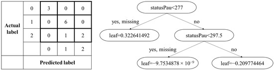
Figure 8.
Confusion matrix (input) and decision tree (output) of XGBoost (six-day period).
Many parameters could be adjusted in XGBoost. However, only certain selected parameters were fine-tuned in this study to provide better results. The selected parameters and their default values were eta (default = 0.3), gamma (default = 0), max_depth (default = 6), min_child_weight (default = 1) and subsample (default = 1). After fine-tuning, we adjusted the parameters to 0.2 for eta, 4.2 for gamma, 5 for max_depth, 1.0 for min_child_weight and 0.5 for the subsample to provide more accurate results.
3.1.5. Machine Classification and Labelling
The machines’ average idle time levels, total number of records, concentrations of abnormal idle time, ratio of adjusting and ratio of pause were determined. Q1 and Q3 were used to define the three levels for all labels. Table 3 shows the machine labelling results.
Table 3.
Machine labelling results.
The results demonstrated that some of the machines had symmetric relationships. That is, when their ratio of pause and average idle time level were level 2 or level 0, their ratio of adjusting and total number of records were level 0 or level 2, respectively. This was the case for machines with MachineIDs 9, 11, 14, 19, 21, 22, 26, 27, 29 and 30. Machines with MachineIDs 9, 11, 14 and 22 recorded low average idle time levels, but their total number of records was high, indicating that these machines always had short idle times. It was also found that the ratio of adjusting was high and the ratio of pause was low, potentially indicating that, for these machines, the adjusting status was the most common status, but lasted for less time, contributing to a lower average idle time. Meanwhile, the average idle time levels for machines with MachineIDs 19, 21, 26, 27, 29 and 30 were high, but the total number of records was low, indicating that it happened rarely, but machine idle times were long when it happened. In addition, if the ratio of adjusting was low, the ratio of pause was high. This indicated that these machines paused more often and for longer, but this did not happen often, thereby contributing to higher average idle times. Furthermore, machines with MachineIDs 1, 2, 15 and 17 had five level one labels, indicating that these four machines were very average. In addition, in terms of the labels’ average idle time level, total number of records and concentration of abnormal idle time levels, the machines with MachineIDs 16 and 18 also received a level one rating, indicating that the two machines were somewhat average. The machines with MachineIDs 6 and 13 were classified as level 0 and level 1, indicating that they were the most efficient. The machine with MachineID 8 documented the worst efficiency, receiving two level two labels and one level one label.
3.2. In-House Transit
As Figure 9 shows, the in-house transit involved five components: ‘Injection to Assembly’, ‘Injection to Warehouse’, ‘Warehouse to Assembly’, ‘Warehouse to Injection’ and ‘Assembly to Warehouse’.
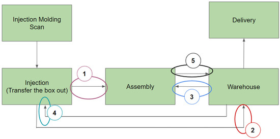
Figure 9.
Illustration of in-house transit processes.
The idle time during the in-house transit processes was analysed using the average (average operation time, denoted by ‘AVG’), the maximum (the worst case during transit, denoted by ‘MAX’), the minimum (the best case during transit, denoted by ‘MIN’), the standard deviation (denoted by ‘SD’) and the above-average percentage (the ratio of data transition time exceeding the average, denoted by ‘>AVG%’).
3.2.1. From the Injection Moulding Workshop to the Assembly Workshop
During the ‘Injection to Assembly’ process, the total number of records was 30,447, the average transportation time was 02:54:49, the maximum transportation time was 121:57:20, the minimum transportation time was 00:00:23, the standard deviation was 08:35:31 and the ratio of data exceeding the average time was 18.55%. For observations of two or more consecutive months, some monthly values were continuously larger or smaller than the whole-year values. From April 2021 to May 2021, the monthly average was continuously larger than the whole-year average. From December 2020 to January 2021 and from August 2021 to September 2021, the monthly average was continuously smaller than the whole-year average. There were no two or more consecutive months that recorded standard deviations continuously larger than the whole-year standard deviation. However, from December 2020 to March 2021, from May 2021 to June 2021 and from August 2021 to November 2021, the monthly standard deviation was continuously smaller than the whole-year standard deviation.
To further improve the accuracy of the analysis, outliers—that is, all data points larger than the upper control limit—were removed from the original data for further processing. After outliers representing an average of approximately 16.03% of the data were removed from each monthly record, the total number of records retained was 25,635; the average transportation time was 00:38:30; the maximum transportation time was 03:33:08; the minimum transportation time was 00:00:23; the standard deviation was 00:46:26; the ratio of data exceeding the average time was 31.15%. For observations of two or more consecutive months, some monthly values were continuously larger or smaller than the whole-year values. From May 2021 to July 2021 and from October 2021 to November 2021, the monthly average was continuously larger than the whole-year average. From February 2021 to April 2021 and from August 2021 to September 2021, the monthly average was continuously smaller than the whole-year average. Regarding the standard deviation, from September 2021 to November 2021, the monthly standard deviation was continuously larger than the whole-year standard deviation. Meanwhile, from February 2021 to March 2021 and from May 2021 to June 2021, the monthly standard deviation was continuously smaller than the whole-year standard deviation.
3.2.2. From the Injection Moulding Workshop to the Warehouse
During the ‘Injection to Warehouse’ process, the total number of records was 357,391, the average transportation time was 02:09:29, the maximum transportation time was 112:24:11, the minimum transportation time was 00:00:20, the standard deviation was 03:05:14 and the ratio of data exceeding the average time was 27.35%. For observations of two or more consecutive months, some monthly values were continuously larger or smaller than the whole-year values. From February 2021 to April 2021 and from June 2021 to August 2021, the monthly average was continuously larger than the whole-year average. From September 2021 to November 2021, the monthly average was continuously smaller than the whole-year average. Regarding the standard deviation, from June 2021 to July 2021, the monthly standard deviation was continuously larger than the whole-year standard deviation. Meanwhile, from December 2020 to January 2021 and from August 2021 to November 2021, the monthly standard deviation was continuously smaller than the whole-year standard deviation.
After outliers representing an average of approximately 23.70% of the data were removed from each monthly record, the total number of records retained was 26,6796; the average transportation time was 00:52:08; the maximum transportation time was 02:23:55; the minimum transportation time was 00:00:20; the standard deviation was 00:34:22; the ratio of data exceeding the average time was 41.78%. For observations of two or more consecutive months, some monthly values were continuously larger or smaller than the whole-year values. From July 2021 to August 2021, the monthly average was continuously larger than the whole-year average. From January 2021 to March 2021, from May 2021 to June 2021 and from September 2021 to October 2021, the monthly average was continuously smaller than the whole-year average. Regarding the standard deviation, from October 2021 to November 2021, the monthly standard deviation was continuously larger than the whole-year standard deviation. Meanwhile, from December 2020 to March 2021, the monthly standard deviation was continuously smaller than the whole-year standard deviation.
3.2.3. From the Warehouse to the Assembly Workshop
During the ‘Warehouse to Assembly’ process, the total number of records was 295,929, the average transportation time was 01:41:24, the maximum transportation time was 95:45:36, the minimum transportation time was 00:00:25, the standard deviation was 07:47:28 and the ratio of data exceeding the average time was 10.27%. For observations of two or more consecutive months, some monthly values were continuously smaller than the whole-year values, but there were no two or more consecutive months that the monthly average was continuously larger than the whole-year average. Nonetheless, from December 2020 to March 2021 and from July 2021 to October 2021, the monthly average was continuously smaller than the whole-year average. There were no two or more consecutive months that recorded standard deviations continuously larger than the whole-year standard deviation. However, from December 2020 to March 2021 and from July 2021 to November 2021, the monthly standard deviation was continuously smaller than the whole-year standard deviation.
After outliers representing an average of approximately 9.66% of the data were removed from each monthly record, the total number of records retained was 26,5748; the average transportation time was 00:08:15; the maximum transportation time was 01:43:14; the minimum transportation time was 00:00:25; the standard deviation was 00:13:49; the ratio of data exceeding the average time was 22.31%. For observations of two or more consecutive months, some monthly values were continuously larger or smaller than the whole-year values. From March 2021 to June 2021, the monthly average was continuously larger than the whole-year average. From December 2020 to February 2021 and from September 2021 to November 2021, the monthly average was continuously smaller than the whole-year average. Regarding the standard deviation, from March 2021 to June 2021, the monthly standard deviation was continuously larger than the whole-year standard deviation. Meanwhile, from January 2021 to February 2021 and from September 2021 to November 2021, the monthly standard deviation was continuously smaller than the whole-year standard deviation.
3.2.4. From the Warehouse to the Injection Moulding Workshop
During the ‘Warehouse to Injection’ process, the total number of records was 2008, the average transportation time was 00:38:00, the maximum transportation time was 81:54:03, the minimum transportation time was 00:00:31, the standard deviation was 02:42:32 and the ratio of data exceeding the average time was 19.87%. For observations of two or more consecutive months, some monthly values were continuously larger or smaller than the whole-year values. From April 2021 to May 2021, the monthly average was continuously larger than the whole-year average. From December 2020 to January 2021 and from June 2021 to September 2021, the monthly average was continuously smaller than the whole-year average. There were no two or more consecutive months that recorded standard deviations continuously larger than the whole-year standard deviation. However, from December 2020 to March 2021 and from May 2021 to September 2021, the monthly standard deviation was continuously smaller than the whole-year standard deviation.
After outliers representing an average of approximately 14.82% of the data were removed from each monthly record, the total number of records retained was 1826; the average transportation time was 00:10:50; the maximum transportation time was 00:44:29; the minimum transportation time was 00:00:31; the standard deviation was 00:13:43; the ratio of data exceeding the average time was 23.55%. For observations of two or more consecutive months, some monthly values were continuously larger or smaller than the whole-year values. From June 2021 to July 2021, the monthly average was continuously larger than the whole-year average. From December 2020 to May 2021 and from August 2021 to October 2021, the monthly average was continuously smaller than the whole-year average. There were no two or more consecutive months that recorded standard deviations continuously larger than the whole-year standard deviation. However, from December 2020 to May 2021 and from July 2021 to October 2021, the monthly standard deviation was continuously smaller than the whole-year standard deviation.
3.2.5. From the Assembly Workshop to the Warehouse
During the ‘Assembly to Warehouse’ process, the total number of records was 188, the average transportation time was 17:31:51, the maximum transportation time was 186:37:39, the minimum transportation time was 00:01:01, the standard deviation was 33:19:54 and the ratio of data exceeding the average time was 48.40%. For observations of two or more consecutive months, some monthly values were continuously smaller than the whole-year values, but there were no two or more consecutive months that the monthly average was continuously larger than the whole-year average. Nonetheless, from March 2021 to April 2021 and from June 2021 to July 2021, the monthly average was continuously smaller than the whole-year average. There were no two or more consecutive months that recorded standard deviations continuously larger than the whole-year standard deviation. However, from January 2021 to March 2021 and from June 2021 to July 2021, the monthly standard deviation was continuously smaller than the whole-year standard deviation.
After outliers representing an average of approximately 4.58% of the data were removed from each monthly record, the total number of records retained was 176; the average transportation time was 10:27:32; the maximum transportation time was 34:03:45; the minimum transportation time was 0:01:01; the standard deviation was 10:27:29; the ratio of data exceeding the average time was 44.89%. For observations of two or more consecutive months, some monthly values were continuously smaller than the whole-year values, but there were no two or more consecutive months that the average was continuously larger than the whole-year average. Nonetheless, from December 2020 to January 2021, from March 2021 to April 2021 and from June 2021 to July 2021, the monthly average was continuously smaller than the whole-year average. There were no two or more consecutive months that recorded standard deviations continuously larger than the whole-year standard deviation. Each month’s standard deviation was smaller than the whole-year standard deviation.
3.2.6. Comparison of All In-House Transit Processes
Due to there being too few records for ‘Assembly to Warehouse’ (only 188 before the removal of outliers and 176 after the removal of outliers) compared to the other in-house transit processes, it was excluded from the comparative analysis. Figure 10 and Figure 11 summarise the transportation data of all in-house transit processes before and after removing outliers. The percentage change in the average transit time for ‘Injection to Assembly’ before and after removing outliers was −77.98%; the percentage change in the average transit time for ‘Injection to Warehouse’ before and after removing outliers was −59.74%; the percentage change in the average transit time for ‘Warehouse to Assembly’ before and after removing outliers was −91.86%; the percentage change in the average transit time for ‘Warehouse to Injection’ before and after removing outliers was −71.49%.
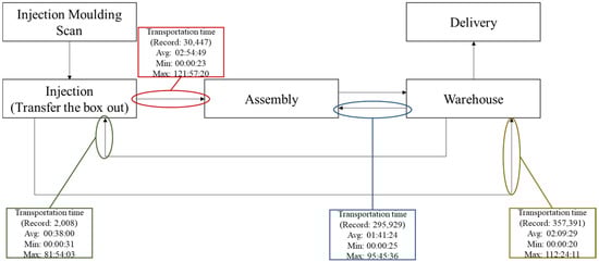
Figure 10.
Transportation time for each in-house transit process before removing outliers.
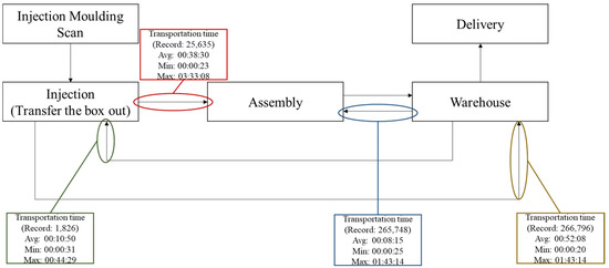
Figure 11.
Transportation time for each in-house transit process after removing outliers.
4. Discussion
The average idle time for each day was calculated as well as the moving average over 15, 20, 30 and 50 days. Then, the standard deviation and variance of the moving average were calculated. The 15-day period demonstrated the highest variance, indicating that this period featured the highest level of sensitivity. Therefore, to balance the workload and sensitivity, it is suggested that the model be updated every 15 days. A 20-day period would also be acceptable for balancing the workload and sensitivity. For the 20-day period, the workload would decrease by 25%, with variance being approximately 11.6% lower. Table 4 shows the data from these different time periods.
Table 4.
Data from the different time periods of interest.
To better utilise the limited resources and time, L.A. could prioritise the machines recording low efficiency levels (based on the ratio of machine running time to machine idle time) and low problem ratios (based on the ratio of machine adjusting time to machine pause time). Efforts should be contributed to investigate the reasons for the low problem ratio.
If L.A. wanted to increase the accuracy of the predictions of abnormal idle time occurrences (output Y), periods of different lengths could be used. For the case study, 80% of the data were used as the training dataset, with a period of six days found to produce the highest accuracy level. Further research could be conducted to improve the accuracy of the predictions by investigating the accuracy in the context of more periods of different lengths to, ultimately, balance the effort and prediction accuracy.
Investigation and improvement priorities should not only be focused on the machine level, but also the in-house transit level. The results of the in-house track and trace revealed that in-house transit type(s) and month(s) with above-average idle time and continuously high idle time could be identified and assigned the highest handling priority. These results enabled L.A. to determine informed decisions and plan for the timely control of the situation.
This study achieved four objectives: The first involved understanding and analysing the data on the idle time of injection moulding machines. This involved conducting a basic statistical analysis of machines’ idle times. Analysing the data before and after removing the outliers, which were defined by the upper control limits, allowed for the determination of the idle times and statuses of the machines. Efficiency levels and potential problems were also explored. Using an efficiency and problem ratio matrix, the machines were compared to determine which needs should be prioritised for each machine (given the limited resources and tight deadlines). The second objective was to determine abnormal idle times. This was achieved by using an indicator to investigate abnormal idle time lengths and demonstrate the occurrence of abnormal idle time over specific time periods. The third objective was to classify different levels of occurrence of abnormal idle times of injection moulding machines. This was achieved by classifying idle times into three levels: high, medium and low. Then, these results were displayed in a confusion matrix and decision tree, which were useful for determining which machines recorded the most occurrences of idle time. In addition, abnormal idle time levels were classified to show the concentration of data for the different machines and months. Furthermore, machine labelling was conducted, showing symmetrical relationships. Accordingly, it was suggested that the manufacturer should update its policies to include an updated indicator of abnormal idle times. A possible period for this oversight was also provided. Nonetheless, due to the limited variables employed, future research is needed. The fourth objective was to indicate the total idle time achieved. The occurrence of abnormal time in the overall track and trace and for each in-house transit process was determined to demonstrate the abnormal idle time.
This study used a limited number of variables due to the data-driven approach employed. That is, only the status was considered. To improve the classification accuracy and generalisability of the results, variables related specifically to injection moulding machines should be included, such as the temperature, pressure and velocity. These were not considered by this study because they were out of scope.
When a spare part in a machine starts to malfunction and needs to be replaced, scheduling a repair is challenging because the change requires some downtime [25]. This study provided insights into analysing idle time without understanding the actual working process, even though it remains feasible to use the machines to facilitate more efficient job scheduling.
5. Conclusions
The automation and data exchange of manufacturing technologies have merged with the industrial IoT to create interconnected manufacturing systems capable of communicating, analysing and using information to drive intelligent actions in the physical world. This study presented a data-driven framework that can be used to statistically analyse raw data across machines to provide a comprehensive understanding of idle time and facilitate machine adjustments to, ultimately, reduce defect rates.
This study provided a quick and practical two-stage data-driven framework to complete the classification. The first stage involved the fundamental statistical analysis of raw data to provide a more comprehensive understanding of idle time and suggest further investigative steps. The second stage involved the identification of indicators and the occurrence of abnormal idle times, as well as the classification of the abnormal idle time of injection moulding machines without consideration of machine parameters.
Thus, this study introduced a new data-driven approach to analysing raw data. To our knowledge, the classification of abnormal idle time without referencing on-site parameters is novel and represents a data-driven method for analysing abnormal idle time that produces insights quickly. In short, idle time levels are tracked with total and abnormal idle times identified. Different levels of abnormal idle time were classified in the case study of a manufacturing site. Due to this being a data-driven approach, automated machine learning and AI approaches did not pertain to the research scope.
This study’s findings represent a framework for analysing raw data and manufacturing processes at an initial stage. Despite significant advancements in fault prediction research, there remains ample room for further exploration and development in this area. This is particularly true given the continuous expansion in the scope and scale of sensor data, creating new opportunities for enhancing the accuracy and applicability of fault prediction models. At present, predicting future faults using collected raw signals is a challenging problem, especially given that data distributions at present and future moments are not guaranteed. Traditional machine learning algorithms can only resolve classification or regression issues within identical data distributions. However, deep learning methods, such as recurrent neural networks (RNNs), convolutional neural networks (CNNs) and transfer learning, can help to predict future faults using the collected raw signal of the present moment, even when the data distributions of present and future moments differ [26,27,28]. The authors plan to design and evaluate these models to ensure their effectiveness and reliability in the context of machine faults and root cause analyses.
Author Contributions
Conceptualisation, C.-H.W. and S.C.-H.N.; methodology, C.-H.W. and S.C.-H.N.; data curation, K.C.-M.K.; formal analysis, C.-H.W. and K.-L.Y.; project administration, K.C.-M.K. and C.-H.W.; writing—original draft preparation, C.-H.W.; writing—review and editing, S.C.-H.N., K.C.-M.K. and K.-L.Y.; funding acquisition, C.-H.W. and K.-L.Y. All authors have read and agreed to the published version of the manuscript.
Funding
This research was partially funded by the University Grants Committee of the HKSAR, China (RMGS project account no.: 700011 and 700043), and the School Research Grant, HSUHK (reference: SDSC-SRG016).
Data Availability Statement
The data presented in this study are available on request from the corresponding author. The data are not publicly available due to the confidentiality of the case company.
Acknowledgments
The authors would like to thank the Department of Supply Chain and Information Management, The Hang Seng University of Hong Kong, the Department of Industrial and Systems Engineering, The Hong Kong Polytechnic University and the case company – L.A. (alias) for supporting the project. Special thanks go to Dr Polly Leung, Mr Samuel Yeung and the MSIM Research Project team #5 (21/22) for their support provided in this project.
Conflicts of Interest
The authors declare no conflict of interest.
References
- Mohamed, N.; Al-Jaroodi, J. Applying blockchain in industry 4.0 applications. In Proceedings of the IEEE 9th Annual Computing and Communication Workshop and Conference, Las Vegas, NV, USA, 6–8 January 2020; pp. 852–858. [Google Scholar]
- Zuo, Y. Making smart manufacturing smarter—A survey on blockchain technology in Industry 4.0. Enterp. Inf. Syst. 2021, 15, 1323–1353. [Google Scholar] [CrossRef]
- Lasi, H.; Kemper, H.-G.; Fettke, P. Industry 4.0. Bise-Catchword 2014, 6, 239–242. [Google Scholar] [CrossRef]
- Tao, F.; Qi, Q.; Wang, L.; Nee, A.Y.C. Digital twins and cyber–physical systems toward smart manufacturing and industry 4.0: Correlation and comparison. Engineering 2019, 5, 653–661. [Google Scholar] [CrossRef]
- Patalas-Maliszewska, J.; Topczak, M. A new management approach based on additive manufacturing technologies and industry 4.0 requirements. Adv. Prod. Eng. Manag. 2021, 16, 125–135. [Google Scholar] [CrossRef]
- Vaidya, S.; Ambad, P.; Bhosle, S. Industry 4.0—A glimpse. Sci.-Procedia Manuf. 2018, 20, 233–238. [Google Scholar] [CrossRef]
- Geng, T.; Du, Y. The business model of intelligent manufacturing with Internet of Things and machine learning. Enterp. Inf. Syst. 2022, 16, 307–325. [Google Scholar] [CrossRef]
- Holdowsky, J.; Mahto, M.; Raynor, M.; Cotteleer, M. Inside the Internet of Things: A Primer on the Technologies Building the IoT; Deloitte University Press: New York, NY, USA, 2015. [Google Scholar]
- Medhi, A.M.; Patange, A.D.; Pardeshi, S.S.; Jegadeeshwaran, R.; Kuntoglu, M. Overview of contemporary systems driven by open-design movement. arXiv 2022, arXiv:2201.05698. [Google Scholar]
- Atzori, L.; Iera, A.; Morabito, G. The Internet of Things: A survey. Comput. Netw. 2010, 54, 2787–2805. [Google Scholar] [CrossRef]
- Raza, A.; Ikram, A.A.; Amin, A.; Ikram, A.J. A review of low cost and power efficient development boards for IoT applications. In Proceedings of the 2016 Future Technologies Conference (FTC), San Francisco, CA, USA, 6–7 December 2016; pp. 786–790. [Google Scholar]
- Sharma, K.; Anand, D.; Mishra, K.K.; Harit, S. Progressive study and investigation of machine learning techniques to enhance the efficiency and effectiveness of industry 4.0. Int. J. Softw. Sci. Comput. Intell. 2022, 14, 1–14. [Google Scholar] [CrossRef]
- Sun, K. Analysis of production and organisational management efficiency of Chinese family intelligent manufacturing enterprises based on IoT and machine learning technology. Enterp. Inf. Syst. 2022, 16, 208–222. [Google Scholar] [CrossRef]
- Farooqui, A.; Bengtsson, K.; Falkman, P.; Fabin, M. Towards data-driven approaches in manufacturing: An architecture to collect sequences of operations. Int. J. Prod. Res. 2020, 58, 4947–4963. [Google Scholar] [CrossRef]
- Rikalovic, A.; Suzic, N.; Bajic, B.; Piuri, V. Industry 4.0 implementation challenges and opportunities: A technological perspective. IEEE Syst. J. 2022, 16, 2797–2810. [Google Scholar] [CrossRef]
- Tran, M.Q.; Doan, H.P.; Vu, V.Q.; Vu, L.T. Machine learning and IoT-based approach for tool condition monitoring: A review and future prospects. Measurement 2023, 207, 112351. [Google Scholar] [CrossRef]
- Fung, V.W.C.; Yung, K.C. An intelligent approach for improving printed circuit board assembly process performance in Smart Manufacturing. Int. J. Eng. Bus. Manag. 2020, 12, 1–12. [Google Scholar] [CrossRef]
- Jintana, J.; Sopadang, A.; Ramingwong, S. Idea selection of new service for courier business: The opportunity of data analytics. Int. J. Eng. Bus. Manag. 2021, 13, 1–20. [Google Scholar] [CrossRef]
- Klingenberg, C.; Borges, M.A.V.; Antunes, J.A.V., Jr. Industry 4.0 as a data-driven paradigm: A systematic literature review on technologies. J. Manuf. Technol. Manag. 2019, 32, 570–592. [Google Scholar] [CrossRef]
- Bajaj, N.S.; Patange, A.D.; Jegadeeshwaran, R.; Pardeshi, S.S.; Kulkarni, K.A.; Ghatpande, R.S. Application of metaheuristic optimization based support vector machine for milling cutter health monitoring. Intell. Syst. Appl. 2023, 18, 200196. [Google Scholar] [CrossRef]
- Chen, T.; Guestrin, C. XGBoost: A scalable tree boosting system. In Proceedings of the 22nd ACM SIGKDD International Conference on Knowledge Discovery and Data Mining, New York, NY, USA, 13–17 August 2016; pp. 785–794. [Google Scholar]
- Patange, A.D.; Pardeshi, S.S.; Jegadeeshwaran, R.; Zarkar, A.; Verma, K. Augmentation of decision tree model through hyper-parameters tuning for monitoring of cutting tool faults based on vibration signatures. J. Vib. Eng. Technol. 2022. [Google Scholar] [CrossRef]
- Loyola-González, O. Black-box vs. white-box: Understanding their advantages and weaknesses from a practical point of view. IEEE Access 2019, 7, 154096–154113. [Google Scholar] [CrossRef]
- Salama, M.; Kader, H.A.; Abdelwahab, A. An analytic framework for enhancing the performance of big heterogeneous data analysis. Int. J. Eng. Bus. Manag. 2021, 13, 1–11. [Google Scholar] [CrossRef]
- Jagan, D.; Senthilvel, A.N.; Prabhakar, R.; Maheswari, S.U. Analysis for maximal optimised penalty for the scheduling of jobs with specific due date on a single machine with idle time. Procedia Comput. Sci. 2015, 47, 247–254. [Google Scholar] [CrossRef]
- Li, Y. A fault prediction and cause identification approach in complex industrial processes based on deep learning. Comput. Intell. Neurosci. 2021, 2021, 6612342. [Google Scholar] [CrossRef] [PubMed]
- Helbing, G.; Ritter, M. Deep Learning for fault detection in wind turbines. Renew. Sustain. Energy Rev. 2018, 98, 189–198. [Google Scholar] [CrossRef]
- Shao, S.; McAleer, S.; Yan, R.; Baldi, P. Highly Accurate Machine Fault Diagnosis Using Deep Transfer Learning. IEEE Trans. Ind. Inform. 2019, 15, 2446–2455. [Google Scholar] [CrossRef]


Disclaimer/Publisher’s Note: The statements, opinions and data contained in all publications are solely those of the individual author(s) and contributor(s) and not of MDPI and/or the editor(s). MDPI and/or the editor(s) disclaim responsibility for any injury to people or property resulting from any ideas, methods, instructions or products referred to in the content. |
© 2023 by the authors. Licensee MDPI, Basel, Switzerland. This article is an open access article distributed under the terms and conditions of the Creative Commons Attribution (CC BY) license (https://creativecommons.org/licenses/by/4.0/).